The Abundance Properties of Nearby Late-Type Galaxies.
II. The Relation between Abundance Distributions and Surface Brightness Profiles

Abstract

The relations between oxygen abundance and disk surface brightness (OH–$SB$ relation) in the infrared $W1$ band are examined for a nearby late-type galaxies. The oxygen abundances were presented in Paper I. The photometric characteristics of the disks are inferred here using photometric maps from the literature through bulge-disk decomposition. We find evidence that the OH – $SB$ relation is not unique but depends on the galactocentric distance $r$ (taken as a fraction of the optical radius $R_{25}$) and on the properties of a galaxy: the disk scale length $h$ and the morphological $T$-type. We suggest a general, four-dimensional OH – $SB$ relation with the values $r$, $h$, and $T$ as parameters. The parametric OH – $SB$ relation reproduces the observed data better than a simple, one-parameter relation; the deviations resulting when using our parametric relation are smaller by a factor of $\sim$1.4 than that the simple relation. The influence of the parameters on the OH – $SB$ relation varies with galactocentric distance. The influence of the $T$-type on the OH – $SB$ relation is negligible at the centers of galaxies and increases with galactocentric distance. In contrast, the influence of the disk scale length on the OH – $SB$ relation is maximum at the centers of galaxies and decreases with galactocentric distance, disappearing at the optical edges of galaxies. Two-dimensional relations can be used to reproduce the observed data at the optical edges of the disks and at the centers of the disks. The disk scale length should be used as a second parameter in the OH – $SB$ relation at the center of the disk while the morphological $T$-type should be used as a second parameter in the relation at optical edge of the disk. The relations between oxygen abundance and disk surface brightness in the optical $B$ and infrared $K$ bands at the center of the disk and at optical edge of the disk are also considered. The general properties of the abundance – surface brightness relations are similar for the three considered bands $B$, $K$, and $W1$.

1 Introduction

The chemical properties of late-type galaxies at the present epoch are described by two values: the gas-phase abundance at a given (predetermined) galactocentric distance (characteristic abundance) and the radial abundance gradient. The value of the oxygen abundance at the $B$-band effective (or half-light) radius of the disk (Garnett & Shields, 1987; Garnett, 2002), the value of the central oxygen abundance extrapolated to zero radius from the radial abundance gradient (Vila-Costas & Edmunds, 1992), the value of the oxygen abundance at $r=0.4R_{\rm 25}$, where $R_{\rm 25}$ is the isophotal (or photometric) radius (Zaritsky et al., 1994), and the value of the oxygen abundance at one disk scale length from the nucleus (Garnett et al., 1997) all have been used as the characteristic oxygen abundance in a galaxy. The slope of the abundance gradient is usually expressed in terms of dex $R_{\rm 25}^{-1}$ or in terms of dex kpc^-1.

The correlations between the characteristic oxygen abundance, the radial abundance gradient, and global, macroscopic properties (such as luminosity, stellar mass, Hubble type, rotation velocity) of spiral and/or irregular galaxies were the subject of many investigations. Lequeux et al. (1979) were the first who revealed that the oxygen abundance correlates with total galaxy mass for irregular galaxies, in the sense that the higher the total mass, the higher the heavy element content. The existence of correlations between the characteristic oxygen abundance and the luminosity (stellar mass, Hubble type, rotation velocity) of nearby late-type (spiral and irregular) galaxies was found by Vila-Costas & Edmunds (1992); Zaritsky et al. (1994); Pilyugin et al. (2004, 2007); Pilyugin & Thuan (2007); Moustakas et al. (2010), and Berg et al. (2012), among many others.

The amount of available spectra of emission-line galaxies has increased significantly because of the completion of several large spectral surveys, e.g., the Sloan Digital Sky Survey (SDSS) (York et al., 2000). Those measurements are used for abundance determinations that provide the extended basis for investigations of the mass (luminosity) – metallicity relation. The existence of the correlation between the characteristic oxygen abundance and the luminosity (stellar mass) was confirmed using many thousands of SDSS galaxies (e.g., Kniazev et al., 2003, 2004; Tremonti et al., 2004; Thuan et al., 2010).

In contrast to the behavior of the characteristic abundance, the slope of the radial abundance gradients does not significantly correlate with the global properties of galaxies (Vila-Costas & Edmunds, 1992; Zaritsky et al., 1994; Sánchez et al., 2014; Pilyugin et al., 2014). According to Zaritsky et al. (1994), the lack of a correlation between gradients and global properties of late-type galaxies may suggest that the relationship between these parameters is more complex than a simple correlation. Indeed, Vila-Costas & Edmunds (1992) have concluded that a correlation is seen for non-barred galaxies.

The only really significant result for understanding the origin of the radial abundance gradients in the disks of late-type galaxies is the correlation found between the local oxygen abundance and the stellar surface brightness or surface mass density (Webster & Smith, 1983; Edmunds & Pagel, 1984; Vila-Costas & Edmunds, 1992; Ryder, 1995; Moran et al., 2012; Rosales-Ortega et al., 2012; Sánchez et al., 2014). The maximum difference in oxygen abundances of H ii regions at similar local stellar surface brightnesses in different galaxies can be as large as $\sim 0.5$ dex (see, e.g., Fig. 9 in Ryder, 1995, as well our data below). The maximum difference in oxygen abundances of H ii regions at similar local surface mass densities is lower, $\sim 0.4$ dex, (Fig. 1 in Rosales-Ortega et al., 2012) with a 1$\sigma$ scatter of the data about the median of $\pm$0.14 dex. We consider this as a hint that the simple ordinary relationship between the abundance and stellar surface brightness can be only a rough approximation and the dependence can vary appreciably both with galactocentric distance within a given galaxy as well as from galaxy to galaxy. In other words, one can expect that a parametric relationship between abundance and surface brightness reproduces the observed data better than the ordinary relation.

In this study we will examine whether the dependence between the abundance and stellar surface brightness varies with galactocentric distance within a given galaxy and from galaxy to galaxy as well as which parameters control those variations. To answer these questions we will examine the relations between the abundance and stellar surface brightness at different galactocentric distances, in particular at the center of the disk and at the isophotal $R_{25}$ radius (or the optical edge) of the disk. Both simple (one-dimensional) relationships between the abundance and stellar surface brightness and parametric (two- and four-dimensional) relationships with different parameters will be considered. Our paper is organized in the following way. We describe the data that were used in Section 2. We examine the abundance – surface brightness diagrams for different samples of galaxies in Section 3. We discuss and summarize our results in Section 4.

2 Data

2.1 Abundances

We investigated the oxygen and nitrogen abundances in the disks of 130 nearby late-type galaxies in Paper I (Pilyugin et al., 2014). We have collected around 3740 published spectra of H ii regions from many studies (see the list of references for the emission line flux measurements in Table 3 in Paper I). Since there are different methods for abundance determinations being used in different works, the resulting abundances from these studies are not homogeneous. Therefore, the oxygen and nitrogen abundances in all H ii regions were redetermined in a uniform way. We investigated the oxygen and nitrogen abundance distributions across the optical disks of those galaxies. In particular, we find the abundances in their centers, (O/H)₀, and at their isophotal $R_{25}$ disk radii, (O/H)${}_{R_{25}}$. It should be emphasized that the (O/H)₀ and (O/H)${}_{R_{25}}$ values are not the abundances in individual H ii regions at the corresponding galactocentric distances (in many galaxies we have no measurements of H ii regions at the center, $r$ = 0, and at the optical edge of a galaxy, $r$ = $R_{25}$), but are determined from the fit to the radial abundance distribution. These (O/H)₀ and (O/H)${}_{R_{25}}$ values form the basis of the current study.

2.2 Surface brightness profiles in the $W1$ band

We constructed the radial surface brightness profiles in the infrared $W1$ band (with isophotal wavelength 3.4 $\mu$m) using the publicly available photometric maps obtained within the framework of the Wide-field Infrared Survey Explorer (WISE) project (Wright et al., 2010). The conversion of the photometric map into the surface brightness profile is performed in several steps:
– Extraction of the image of a galaxy from the Image Mosaic Service.
– Interactive sky background subtraction.
– Interactive rejection of pixels with bright stars and background galaxies.
– Fitting the surface brightness by ellipses using the task isophote of the package stsdas in iraf where the center of the ellipses is fixed, while the major axis position angle and ellipticity are free parameters. Initial values of the position angle and ellipticity were taken from Paper I.
– Interactive determination of the mean values of the major axis position angle and ellipticity from data of the previous step.
– Derivation of the surface brightness profile using the task isophote of the package stsdas with fixed ellipse center position, position angle, and ellipticity parameters.
In this manner we determined the surface brightness profile, position angle, and ellipticity in the $W1$ band for each galaxy. It should be noted that $WISE$ images in the $W1$ band have an angular resolution of 6.1 arcsec (Wright et al., 2010). Therefore, on the one hand, very small (point-like) bulges can be missed. On the other hand, the bulge size can be overestimated. The $WISE$ survey in the $W1$ band is deep enough to ensure that the surface brightness profiles extend to the optical isophotal radii $R_{25}$ and even beyond those for many galaxies.

All surface brightness measurements were corrected for Galactic foreground extinction before further analysis and interpretation. The measurements were corrected using the $A_{V}$ values from the recalibration by Schlafly & Finkbeiner (2011) of the maps of Schlegel et al. (1998) and the extinction curve of Cardelli et al. (1989), assuming a ratio of total to selective extinction of $R_{V}$ = $A_{V}$/$E_{B-V}$ = 3.1. The $A_{V}$ values given in the NASA Extragalactic Database ned were used. We did not attempt to correct for the intrinsic extinction of the target galaxies.

Surface brightness measurements in solar units were used for the analysis. The magnitude of the Sun in the $W1$ band is obtained from its magnitude in the $V$ band and the color of the Sun $(V-W1)_{\sun}$ = 1.608 taken from Casagrande et al. (2012). The distances to the galaxies were taken from Paper I.

2.3 Bulge-disk decomposition

Exponential profiles of the form

$$\Sigma_{L_{d}}(r)=(\Sigma_{L})_{0}\exp(-r/h),$$ (1)

were used to fit the observed disk surface brightness profiles in the $W1$ band where $(\Sigma_{L})_{0}$ is the central disk surface brightness and $h$ the radial scale length. The bulge profiles were fitted with a general Sérsic profile,

$$\Sigma_{L_{b}}(r)=(\Sigma_{L})_{e}\exp\{-b_{n}[(r/r_{e})^{1/n}-1]\},$$ (2)

where $(\Sigma_{L})_{e}$ is the surface brightness at the effective radius $r_{e}$, i.e., the radius that encloses 50% of the bulge light. The factor $b_{n}$ is a function of the shape parameter $n$. It can be approximated by $b_{n}\approx 1.9992n-0.3271$ for $1<n<10$ (Graham, 2001). Thus, the $W1$ stellar surface brightness distribution within a galaxy was fitted with the expression

$$\begin{array}[]{lll}\Sigma_{L}(r)&=&(\Sigma_{L})_{e}\exp\{-b_{n}[(r/r_{e})^{1/n}-1]\}\\ &+&(\Sigma_{L})_{0}\exp(-r/h).\\ \end{array}$$ (5)

The fit via Eq. (5) will be referred to below as the pure exponential disk (PED) approximation.

The parameters $(\Sigma_{L})_{e}$, $r_{e}$, $n$, $(\Sigma_{L})_{0}$, and $h$ were determined by looking for the best fit to the observed radial surface brighness profile. We wish to derive a set of parameters in Eq. (5) which minimizes the deviation $\sigma_{PED}$ of

$$\sigma=\sqrt{[\sum\limits_{j=1}^{n}(L(r_{j})^{cal}/L(r_{j})^{obs}-1)^{2}]/n}.$$ (6)

Here $L(r_{j})^{cal}$ is the surface brightness at the galactocentric distance $r_{j}$ computed through the Eq. (5) and $L(r_{j})^{obs}$ is the measured surface brightness at that galactocentric distance.

The obtained radial profiles of the disk components were reduced to a face-on galaxy orientation and the bulge components were assumed to be spherical. Note that the inclination correction is purely geometrical, and it does not include any correction for inclination-dependent internal obscuration.

Pohlen & Trujillo (2006) found that only around 10 – 15% of all spiral galaxies have a normal/standard purely exponential disk while the surface brightness distribution of the rest of the galaxies is better described as a broken exponential. Therefore, the $W1$ stellar surface brightness distribution within a galaxy was also fitted with the broken exponential

$$\begin{array}[]{lll}\Sigma_{L}(r)&=&(\Sigma_{L})_{e}\exp\{-b_{n}[(r/r_{e})^{1/n}-1]\}\\ &+&(\Sigma_{L})_{0,inner}\exp(-r/h_{inner})\;\;\;\;if\;\;\;r<R^{*},\\ &=&(\Sigma_{L})_{e}\exp\{-b_{n}[(r/r_{e})^{1/n}-1]\}\\ &+&(\Sigma_{L})_{0,outer}\exp(-r/h_{outer})\;\;\;\;if\;\;\;r>R^{*}.\\ \end{array}$$ (11)

Here $R^{*}$ is the break radius, i.e., the radius at which the exponent is changed. The fit via Eq. (11) will be referred to below as the broken exponential disk (BED) approximation. In this case, eight parameters $(\Sigma_{L})_{e}$, $r_{e}$, $n$, $(\Sigma_{L})_{0,inner}$, $h_{inner}$, $(\Sigma_{L})_{0,outer}$, $h_{outer}$, and $R^{*}$ were determined by looking for the best fit to the observed radial surface brighness profile, i.e., we again require that the deviation $\sigma_{BED}$ given by Eq. (6) is minimized.

Figure 1: The resulting patterns of the bulge-disk decomposition of some of our target galaxies. Each galaxy is presented in two panels. Each upper panel $x1$ shows the decomposition assuming a pure exponential for the disk (with “$x$” running from the letters $a$ to $i$). The measured surface profile is plotted using circles. The bulge contribution is shown by a dotted line, the disk contribution by a dashed line, and the total (bulge + disk) fit by a solid line. Each lower panel $x2$ shows the decomposition assuming a broken exponential for the disk. The bulge contribution is marked by a dotted line, the inner disk by a long-dashed line, the outer disk by a short-dashed line, and the total (bulge + disk) fit by a solid line.

Figure 1 shows the results of the bulge-disk decomposition of some of our galaxies. Each galaxy is displayed in two panels. Each upper panel $x1$ shows the decomposition assuming a pure exponential for the disk. “$x$” stands here for the letters $a$ to $i$, which are used to name the different panels in this figure. The measured surface profile is marked by circles. The fit to the bulge contribution is shown by a dotted line, the fit to the disk by a dashed line, and the total (bulge + disk) fitting by a solid line. Each lower panel $x2$ shows the decomposition assuming a broken exponential for the disk. The bulge contribution is shown by a dotted line, the inner disk by a long-dashed line, the outer disk by a short-dashed line, and the total (bulge + disk) fitting by a solid line.

Table 1 lists the parameters of the surface brightness profiles of our galaxies in the $W1$ band obtained through the bulge-disk decomposition with the PED approximation. The first column contains the galaxy’s name, i.e., its number in the New General Catalogue (NGC), Index Catalogue (IC), Uppsala General Catalog of Galaxies (UGC), or Catalogue of Principal Galaxies (PGC). The galaxy inclination and the position angle of the major axis in the $W1$ band obtained here are given in columns 2 and 3, respectively. The parameters of the general Sérsic profile for the bulge are listed in columns 4 – 6: the logarithm of the bulge surface brightness at the effective radius $r_{e}$ in the $W1$ band in $L_{\sun}$ pc^-2 is reported in column 4, the bulge effective radius in kpc is listed in column 5, and the shape parameter $n$ is given in column 6. The logarithm of central surface brightness of the disk in the $W1$ band in terms of $L_{\sun}$ pc^-2 is listed in column 7. The disk scalelength in the $W1$ band, $h_{W1}$ in kpc, is reported in column 8. The bulge contribution to the galaxy luminosity is reported in column 9. The galaxy luminosity is given in column 10. The mean deviation in the surface brightness $\sigma_{PED}$ around the fit through the bulge-disk decomposition assuming a pure exponential for the disk is given in column 11. The mean deviation $\sigma_{BED}$ assuming a broken exponential for the disk is listed in column 12.

Figure 2: Quality of the surface brightness profile fit obtained via the bulge-disk decomposition. The mean deviation $\sigma_{BED}$ of the fit assuming a broken exponential disk is plotted versus the mean deviation $\sigma_{PED}$ of the fit assuming a pure exponential disk. The dotted line shows equal values.

The accuracy of the surface brightness profile fitting through the bulge-disk decomposition assuming a pure exponential for the disk is specified by the mean deviation $\sigma_{PED}$. The accuracy assuming a broken exponential for the disk is specified by the mean deviation $\sigma_{BED}$. Figure 2 shows the comparison between the mean deviations $\sigma_{PED}$ and $\sigma_{BED}$. The surface brightness profiles of a number of galaxies are well fitted both with the pure and with the broken exponential disks. The mean deviation $\sigma_{PED}$ is small and close to the mean deviation $\sigma_{BED}$. The panels $a$ and $b$ of Figure 1 show the surface brightness profile fitting for two of these galaxies: NGC 628 (with $\sigma_{PED}$ = 0.041 and $\sigma_{BED}$ = 0.034) and NGC 2336 (with $\sigma_{PED}$ = 0.045 and $\sigma_{BED}$ = 0.035). The galaxy NGC 2336 has the largest disk scale length of around 8 kpc among the galaxies of our sample (if the adopted distance to this galaxy is correct).

The surface brightness profiles of a number of galaxies are much better fitted with broken exponential disks than with pure exponential disks. The mean deviation $\sigma_{PED}$ is appreciably larger than the mean deviation $\sigma_{BED}$. Panels $c$, $d$, and $e$ of Figure 1 show the surface brightness profile fitting for three of these galaxies: NGC 2441 (with $\sigma_{PED}$ = 0.136 and $\sigma_{BED}$ = 0.018), NGC 3631 (with $\sigma_{PED}$ = 0.174 and $\sigma_{BED}$ = 0.049), and NGC 5194 (with $\sigma_{PED}$ = 0.129 and $\sigma_{BED}$ = 0.055). The galaxy NGC 3631 has the largest value of the mean deviation $\sigma_{PED}$. Galaxies with strongly broken exponential disks (with a large difference between the disk scale lengths inside and otside the break point) belong to this group of galaxies. Galaxies with bright spiral arms starting at the ends of the bar also belong to this group.

The surface brightness profiles of a number of galaxies are not well fitted with either pure exponential disks nor with broken exponential disks. Their mean deviations $\sigma_{PED}$ and $\sigma_{PED}$ are large. The panels $f$ and $g$ of Figure 1 show the surface brightness profile fitting results for two examples of such galaxies: NGC 1097 (with $\sigma_{PED}$ = 0.129 and $\sigma_{BED}$ = 0.100) and NGC 4321 (with $\sigma_{PED}$ = 0.126 and $\sigma_{BED}$ = 0.075).

In several cases, we could not determine a reliable disk scale length $h_{W1}$ and/or central surface brightness of the disk $(\Sigma_{L_{W1}})_{0}$. The panels $h$ and $i$ of Figure 1 show the surface brightness profile fitting for two examples of such galaxies: NGC 5055 and NGC 7918. The formal values of the mean deviations $\sigma_{PED}$ and $\sigma_{BED}$ can be rather small: $\sigma_{PED}$ = 0.045 and $\sigma_{BED}$ = 0.038 for NGC 5055 and and $\sigma_{PED}$ = 0.038 and $\sigma_{BED}$ = 0.028 for NGC 7918. However, the disk contribution to the surface brightness is close to the observed surface brightness profile over a small interval of radial distances (if any) only (in fact, this is a bulge-dominated galaxy). Therefore, the values of the disk scale length and/or central surface brightness of the disk are questionable. Those galaxies were thus excluded from further consideration.

Our final list involves 95 galaxies with estimates of the disk scale length $h_{W1}$ and central surface brightness of the disk $(\Sigma_{L_{W1}})_{0}$ in the $W1$ band.

2.4 Comparison to other studies

Figure 3: Comparison between disk scale lengths in the $W1$ $WISE$ band with the isophotal wavelength at 3.4 $\mu$m (this study) and in the 3.6 $\mu$m band of the Spitzer Survey of Stellar Structure in Galaxies (Muñoz-Mateos et al., 2013) (see text). The dotted line shows equal values.

Muñoz-Mateos et al. (2013) have analyzed the surface brightness profiles in a sample of nearby disk galaxies using deep $IRAC-1$ (3.6 $\mu$m) images from the Spitzer Survey of Stellar Structure in Galaxies (S ⁴G). There are a number of galaxies in common with our study. Since the isophotal wavelength of the $W1$ $WISE$ band (3.4 $\mu$m) is close to that of $IRAC-1$ S ⁴G we can compare the resulting disk scale lengths from our study and from Muñoz-Mateos et al. (2013). Since we will use the disk scale length derived with the pure exponential disk approximation in our further analysis we will focus on these values. Muñoz-Mateos et al. (2013) have used both pure exponential disks as well as broken exponential disks in their fits, but they reported only their results for the case of the broken exponential disk approximation, i.e., the values of the disk scale length inside and outside of the break point.

In a number of galaxies no disk break was detected. For those galaxies single disk scale lengths were reported. There are four such galaxies in common with our sample. To enlarge the comparison sample of galaxies, their inner disc scale length was considered as a global disk scale length (and compared with our disk scale length obtained with the PED approximation) if the galactocentric distance of the break point exceeds the inner disk scale length by a factor of $\sim$4.

Figure 3 shows the comparison between our disk scale lengths and those from Muñoz-Mateos et al. (2013) for ten galaxies. Figure 3 shows that the our disk scale lengths are in satisfactory agreement (average difference $\sim$ 9%) with the ones from Muñoz-Mateos et al. (2013).

2.5 Data in the $B$ and $K$ bands

We also compile the radial surface brightness profiles in the photometric $B$ and $K$ bands for galaxies of our sample. In some cases we have used published surface brightness profiles (e.g., data from de Jong & van der Kruit (1994); Jarrett et al. (2003); Muñoz-Mateos et al. (2009); Li et al. (2011)). When only photometric maps of galaxies were available (e.g., $B$ and $K$ photometric maps of Knapen et al. (2004), or $g$ and $r$ photometric maps of SDSS DR9 (Ahn et al., 2012)) then the radial surface brightness profiles were determined in the way described above. Position angle and inclination angle of a given galaxy were taken from Paper I and were kept fixed for isophotes at all galactocentric distances. The measurements in the SDSS filters $g$ and $r$ were converted to $B$-band magnitudes, and the $AB$ magnitudes were reduced to the Vega photometric system using the conversion relations and solar magnitudes of Blanton & Roweis (2007). Radial surface brightness profiles in the photometric $B$ and $K$ bands were found for 32 galaxies listed in Table 1.

Table The Abundance Properties of Nearby Late-Type Galaxies. II. The Relation between Abundance Distributions and Surface Brightness Profiles lists the characteristics of the disk in the $B$ and $K$ bands for each galaxy obtained through the bulge-disk decomposition with the PED approximation. The first column contains the galaxy name, i.e., its number in the New General Catalogue. The logarithm of the central surface brightness of the disk in the $B$ band, ($\Sigma_{L_{B}}$)₀ in units of $L_{\sun}$ pc^-2, is given in column 2. The disk scalelength in the $B$ band, $h_{B}$ in kpc, is reported in column 3. The reference to the source for the $B$ band measurements (observed surface brightness profiles or photometric maps of galaxies) used here for the bulge-disk decomposition, i.e., for the determination of the ($\Sigma_{L_{B}}$)₀ and $h_{B}$ values (columns 2 and 3) is given in column 4. The logarithm of the central surface brightness of the disk in the $K$ band, ($\Sigma_{L_{K}}$)₀ in terms of $L_{\sun}$ pc^-2, is listed in column 5. The disk scalelength in the $K$ band, $h_{K}$ in kpc, is reported in column 6. The reference to the source for the $K$-band measurements used for the determination of the ($\Sigma_{L_{K}}$)₀ and $h_{K}$ (columns 5 and 6) via bulge-disk decomposition is given in column 7.

It should be noted that in many cases reliable surface brightness measurements in the $K$ or/and $B$ band do not extend to the isophotal radius $R_{25}$ taken from the Third Reference Catalog ($RC3$, de Vaucouleurs et al (1991)). The measurements become too noisy or are missing beyond some radius.

3 The relation between abundance and surface brightness of the disk

3.1 Preliminary remarks

The relation between abundance and surface brightness of the disk (or surface mass density) was considered in a number of studies (Webster & Smith, 1983; Edmunds & Pagel, 1984; Vila-Costas & Edmunds, 1992; Ryder, 1995; Moran et al., 2012; Rosales-Ortega et al., 2012; Sánchez et al., 2014). There are two approaches to the investigation of the relation between abundance and surface brightness in disks of galaxies (the OH – $SB$ relation) or the relation between abundance and disk surface mass density. The first approach is to compare the local abundance with the local surface brightness (local mass density). But since the measured surface brightness of the central part of a galaxy is the sum of the bulge and disk brightnesses, the relation between measured local abundance and local surface brightness cannot be interpreted as a relation between disk parameters. Another approach is to compare the parameters of the radial abundance distribution with the parameters of the surface brightness profile of the disk derived within the framework of the adopted models.

We follow the latter approach and adopt the simplest (single exponential) model for the abundance and for the surface brightness distributions across the disk. The disk surface brightness distribution is obtained through the bulge-disk decomposition of the measured surface brightness of the galaxy. The advantage of this model is that the radial distribution of metallicity and surface brightness within the framework of the model can be specified by only two parameters in two ways. First, the radial distribution of the abundance (surface brightness) can be characterized by the value of the abundance (surface brightness) at the center of the disk and by the radial abundance gradient (surface brightness disk scale length). Second, the radial distribution of the abundance (surface brightness) can be described by the values of the abundance (surface brightness) at the center of the disk and at the optical edge of a galaxy’s $R_{25}$ isophotal radius. The numerical values of the three parameters (the oxygen abundance, 12+log(O/H), the surface brightness of the disk, log$\Sigma_{L}$, and the disk scale length in kpc, $h$) are comparable to each other within an order of magnitude. The value of the physical radial abundance gradient in terms of dex per kpc is around 2 to 3 orders of magnitude smaller than the above parameters. Therefore, it is preferable to use the second description of the radial abundance distributions (by the values of the abundance at the center of the disk and at the optical edge of a galaxy’s $R_{25}$ isophotal radius) when investigating the relation between abundance and surface brightness distributions. Another strong argument in favor of the use of the abundance at the center and at the optical edge of the disk instead of the radial abundance gradient will be given below.

This approach requires that the adopted models for the abundance distribution and for the surface brightness profile reproduce adequately the observed distributions. The validity of a single exponential distribution of the abundances across the optical disk (the existence of a break in the slope of abundance gradients) has been questioned in a number of studies (Zaritsky, 1992; Vila-Costas & Edmunds, 1992; Scarano & Lépine, 2013; Sánchez et al., 2014, among others). On the other hand, it is well known that the commonly used calibrations for abundance determinations in H ii regions do not work well over the whole range of metallicities, e.g., the $R_{3}N_{2}$ calibration (Marino et al., 2013, and references therein). It has been argued that the use of such calibrations beyond the workable range of metallicities can result in artificial bends (Pilyugin, 2001, 2003). From this point of view the existence of such bends in the slopes of radial abundance gradients in the disks of spiral galaxies may be questioned.

We emphasize that we only consider the abundance distribution within the optical edge of a galaxy’s $R_{25}$ isophotal radius. Radial abundance distributions extending beyond this isophotal radius in the disks of some spiral galaxies have been measured recently (Bresolin et al., 2009, 2012; Goddard et al., 2011) where a shallower oxygen abundance gradient in the outer disk (beyond the isophotal radius) than in the inner disk was found. This discontinuity in the gradient that occurs in proximity of the optical edge of the galaxy seems to be real.

In Paper I the radial oxygen abundance distribution across the optical disk in every galaxy is fitted by a single exponential relation. It looks like a rather good approximation for the majority of the galaxies, at least as a first-order approximation. Indeed, the mean deviations in oxygen abundances around the radial abundance gradient are usually lower than the expected precision (around 0.1 dex) of the abundance determinations in individual H ii regions (see Figure 4). However, a small change in slope in the abundance distribution cannot be excluded in the disks of a number of galaxies (e.g., in NGC 925, NGC 3184, NGC 5457).

As mentioned above, we found that the surface brightness distributions of disks of many galaxies can be well fitted by a pure exponential while the surface brightness distribution of the rest of the galaxies is better described by a broken exponential.

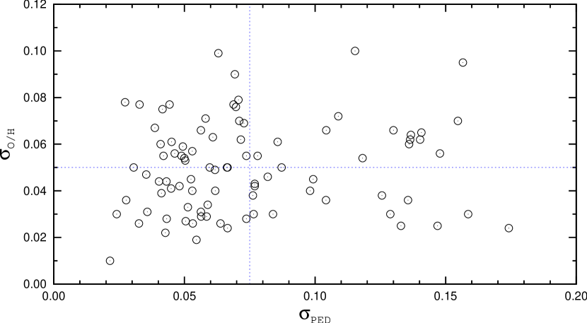
Figure 4: The deviation in oxygen abundances around the radial abundance gradient (in dex) versus the deviation in surface brightness (Eq. (6)) around the surface brightness profile fit assuming a pure exponential for the disk. Dotted lines show the average values of the deviations.

Figure 4 shows the mean deviation in oxygen abundances, $\sigma_{\rm O/H}$, around the radial abundance gradient (in dex) taken from Paper I versus the mean deviation in surface brightness, $\sigma_{PED}$, around the surface brightness profile fit assuming the pure exponential disk from Table 1. If the correlation between local values of metallicity and surface brightness in the disk of a given galaxy is much tighter than the correlation between the global distributions of those parameters or if the single exponential model for the abundance and/or for the surface brightness distributions across the disk of a given galaxy is too uneven then one can expect that a large value of $\sigma_{\rm O/H}$ should be accompanied by a large value of $\sigma_{PED}$, i.e., there should be correlations between the mean deviation in oxygen abundances and the mean deviation in surface brightness. Inspection of Figure 4 shows that there is no such correlation. This may be considered as evidence in favor of single exponential models for the abundance and for the surface brightness distributions across the disks of galaxies being acceptable at least as a zero-order approximation. Another test of the validity of the use of the single exponential models for the abundance and for the surface brightness distributions across the disks of galaxies will be presented below.

3.2 Expected secondary parameters in the OH–$SB$ relationship

We suggest that a simple, single-parameter OH–$SB$ relationship can be only a rough approximation and that the OH–$SB$ dependence can vary appreciably both with galactocentric distance within a given galaxy as well as from galaxy to galaxy. In other words, one can expect that a parametric OH–$SB$ relationship reproduces the observed data better than a simple linear relation.

Which parameters may be considered as possible second parameters in the OH–$SB$ relationship? It is believed that the gas infall rate onto the disk decreases exponentially with time (Matteucci & François, 1989; Pilyugin & Edmunds, 1996a, b; Calura et al., 2009; Pipino et al., 2013, and references therein). The timescale of gas accretion is assumed to increase with radius. This results in an inside-out evolution of the disks of spiral galaxies (Matteucci & François, 1989; Muñoz-Mateos et al., 2011; Gonzalez Delgado et al., 2014). In this scenario the star formation history in the disk can be described by the expression

$$SFR(t,r)\propto A\exp{-{\frac{t}{\tau(r)}}}$$ (12)

In this relation, $\tau$$(r)$ is the timescale of the star formation rate at a given galactocentric distance, and $A$ is the scale factor. The $\tau$$(r)$ value increases smoothly along the radius of the disk. The amount of gas converted into stars at a given radius (and, consequently, the stellar surface mass density and the astration level) can be deduced by integrating the star formation rate over the galaxy lifetime. In turn, the abundance is also defined by the astration level. Then both the radial distributions of the stellar surface mass density and the heavy element content are governed by the same parameters, namely $\tau$$(r)$ and $A$. This results in a correlation between abundance and surface brightness in each individual galaxy. Violent events (merging, interactions) in the evolution of a galaxy in the recent past can affect the properties of the galaxy, e.g., strongly interacting galaxies can undergo a flattening of their gas-phase metallicity gradient (Rupke et al., 2010b).

Thus, the radial distributions of the stellar surface mass density and astration level (and, consequently, abundance) are governed by the same parameters, $\tau$$(r)$ and $A$. This results in the correlation between those characteristics within the disk of an individual galaxy. In particular, the local surface mass density (or surface brightness) can serve as a surrogate indicator of the local abundance in the individual galaxy. Since the $\tau$$(r)$ value varies with radius one can expect that the OH–$SB$ dependence also changes with radius. Since the $\tau$$(r)$ and/or $A$ values vary from one galaxy to another this should result in differences in the OH–$SB$ dependence for different galaxies.

The disk scale length reflects the variation of the star formation history with galactocentric distance. The disk scale length may then be considered as possible second parameter in the OH–$SB$ dependence. It has been known for a long time that the morphological Hubble type of a galaxy, expressed in the terms of $T$-type, is an indicator of the star formation history in a galaxy (Sandage, 1986). Therefore, one may expect that the morphological type is a possible second parameter in the OH–$SB$ dependence. Furthermore, bulge stars contribute to the enrichment of the gas in heavy elements. Hence the bulge contribution to the galaxy luminosity may be also considered as possible second parameter in the OH–$SB$ dependence, especially at the disk center. Figure 5 shows that those three parameters are independent for our sample of galaxies.

Figure 5: Bulge contribution $f_{B}$ to the galaxy luminosity in the $W1$ band (panel $a$) and morphological $T$ type (panel $b$) as a function of the disk scale length $h_{W1}$ in the $W1$ band, and ratio of disk radius to the disk scale length $R_{25}/h_{W1}$ as a function of morphological $T$ type (panel $c$).

We will examine below whether the OH–$SB$ dependence varies with galactocentric distance within a given galaxy and from galaxy to galaxy as well as which parameters control those variations. To address these questions we will examine the relations between the abundance and stellar surface brightness at different galactocentric distances. Both simple (one-dimensional) relationships between the abundance and stellar surface brightness and parametric (two- and four-dimensional) relationships with different parameters will be considered. Firstly, the relations at the center of the disk and at optical edge of the disk will be investigated.

Figure 6: Histograms of morphological $T$ types (panel $a$), disk scale lengths in the $W1$ $WISE$ band (panel $b$), optical radii $R_{25}$ (panel $c$), central oxygen abundances 12 + log(O/H)₀ (panel $d$), and radial oxygen abundance gradients (panel $e$) for our sample of galaxies.

Here we summarize the properties of our sample of galaxies. Figure 6 shows histograms of morphological $T$ types (panel $a$), disk scale lengths in the $W1$ $WISE$ band (panel $b$), optical radii $R_{25}$ (panel $c$), central oxygen abundances 12 + log(O/H)₀ (panel $d$), and radial oxygen abundance gradients (panel $e$) for our sample of galaxies. The optical radii of our galaxies range from $\sim$5 kpc to $\sim$30 kpc, but galaxies with radii between 10 and 18 kpc occur most frequently. The disk scale lengths in the $W1$ $WISE$ band range from $\sim$ 1 kpc to $\sim$ 6 kpc with a few exceptions. The central oxygen abundances of most of the galaxies have values between 12 + log(O/H)₀ = 8.4 and 12 + log(O/H)₀ = 8.9. The radial oxygen abundance gradients expressed in dex kpc^-1 lie within the range of $-0.05$ to 0 although a few galaxies show steeper radial abundance gradients of up to $-0.1$ dex kpc^-1 or even more.

Panel $a$ of Figure 6 shows that our sample includes different numbers of galaxies of different morphological types, in the sense that the Sc galaxies ($T$ = 5) are more numerous than the Sb ($T$ = 3) or Sd ($T$ = 7) galaxies. If the OH–$SB$ relation is dependent on the morphological type of a galaxy and if we will consider the single-parameter OH–$SB$ relation for all galaxies then the fact of unequal numbers of galaxies of different morphological types in a sample will influence the result, in the sense that the derived relation will be biased towards the OH–$SB$ relation for Sc galaxies. Since we will take into account the variation of the OH–$SB$ relation with galaxy properties (in particular, we will consider the parametric OH–$SB$ relation where the morphological type is a parameter) then the fact of unequal numbers of galaxies of different morphological types in a sample will not influence the result. One can say that we will establish the individual relation for galaxies of each morphological type. Thus, it is not necessary to use any selection criteria in the preparation of our sample of galaxies. Therefore, we will consider all the galaxies with available data.

It can be also noted that the use of our entire sample of spiral galaxies and of a subsample of galaxies with pure exponential disks in the determination of the OH–$SB$ relation does not change the general picture (see below). It can be considered as indirect evidence supporting that the selection does not influence the result.

3.3 The relation between central abundance and central surface brightness

Our sample of the surface brightness profiles in the $W1$ band is larger in number than that in the $B$ and $K$ bands. In addition, these data are homogeneous both from the point of view of observations and reduction. Therefore we start the study of the OH–$SB$ relation using the surface brightness in the $W1$ band. We will consider a sample of spiral galaxies with morphological $T$-type 0.5 $\lesssim$ $T$ $\lesssim$ 7.5. This sample comprises 90 galaxies.

Figure 7: Central oxygen abundance as a function of central surface brightness of the disk in the $W1$ band. The dotted line in each panel shows the simple relation (Eq. (13)). Panel $a$ shows the subdivision of our sample of galaxies into three subsamples according to the value of disk scale length $h_{W1}$. The solid line corresponds to the parametric relation O/H=$f({\Sigma}_{L_{W1}},h_{W1})$ (Eq. (14)) for $h_{W1}$ = 1 kpc. The dashed line is the relation for $h_{W1}$ = 7 kpc. Typical errors are shown by the cross in the lower left corner. Panel $b$ shows the subdivision of our sample of galaxies into three subsamples according to the value of the bulge contribution $f_{B}$ to the total galaxy luminosity. The solid line corresponds the parametric relation O/H=$f({\Sigma}_{L_{W1}},f_{B})$ (Eq. (15)) for $f_{B}$ = 0. The dashed line shows the corresponding relation for $f_{B}$ = 1. Panel $c$ shows the subdivision of our sample of galaxies into three subsamples according to the morphological $T$ type. The solid line corresponds to the parametric relation O/H=$f({\Sigma}_{L_{W1}},T)$ (Eq. (16)) for $T$ = 1. The dashed line represents the relation for $T$ = 7.

Figure 8: Panel $a$ shows deviations of the central oxygen abundances from the one-dimensional O/H – $SB$ relation (the residuals of Eq. (13)) as a function of the uncertainty in central oxygen abundance. Panels $b$ shows deviations of the oxygen abundances at the isophotal $R_{25}$ radius of a galaxy from the one-dimensional O/H – $SB$ relation (the residuals of Eq. (20)) as a function of the uncertainty in the oxygen abundances. The points show the values of the individual galaxies. The dotted lines indicate residuals of zero.

Figure 7 shows the central oxygen abundance 12+log(O/H)₀ as a function of central surface brightness of the disk ($\Sigma_{L_{W1}}$)₀ in the $W1$ band. The simple (one-dimensional) linear best fit relation

$$12+\log{\rm(O/H)}_{0}=0.259\,(\pm 0.035)\,\log(\Sigma_{L_{W1}})_{0}+7.91(\pm 0.10)$$ (13)

is shown by the dotted line. The mean deviation around this relation is 0.113. The maximum difference in oxygen abundances at similar local stellar surface brightnesses in different galaxies is as large as $\sim 0.5$ dex, similar to that in previous studies (e.g., Fig. 9 in Ryder, 1995). Typical errors are shown by the cross in the lower left corner. The typical (mean) uncertainty in the central oxygen abundances (0.04 dex) is taken from Paper I. The typical uncertainty in the surface brightnesses (17% or 0.075 dex) is taken as the sum of the mean deviation $\sigma_{PED}$ of the fit assuming a pure exponential disk and the average difference between our disk scale lengths and those from Muñoz-Mateos et al. (2013). It should be noted that the error in the central oxygen abundance is more crucial than the error in the surface brightness. The error in the abundance is directly involved in the deviation of the object from the OH – $SB$ relation while the error in the surface brightness affects the coefficient by up to $\sim$ 0.3 (see the equations of the OH – $SB$ relations).

Panel $a$ in Figure 8 shows the residuals of Eq. (13) as a function of the uncertainty in the central oxygen abundances taken from Paper I. On the one hand, the residuals for objects with small uncertainties in the central oxygen abundances can be large. On the other hand, the residuals for objects with large uncertainties in the central oxygen abundances can be small. This suggests that the deviations around the OH–$SB$ relation at the centers of galaxies cannot be attributed just to the uncertainties in the central oxygen abundances.

Figure 9: The residuals of Eq. (13) (panels $a$, $b$, and $c$) and Eq. (20) (panels $d$, $e$, and $f$) as a function of the disk scale length $h_{W1}$, bulge contribution to the total luminosity $f_{B}$, and morphological $T$ type. The points show the values of the individual galaxies. The dotted lines indicate residuals of zero.

Figure 9 shows the residuals of Eq. (13) as a function of the disk scale length $h_{W1}$ (panel $a$), of the bulge contribution to the total luminosity $f_{B}$ (panel $b$), and of the morphological $T$ type (panel $c$). The residuals are in excess of the typical error in the abundance determinations. Figure 9 suggests that the residuals correlate rather tightly with the disk scale length.

Panel $a$ of Figure 7 shows the subdivision of our sample of galaxies into three subsamples according to the value of the disk scale length $h_{W1}$. The parametric (two-dimensional) best-fit relation is

$$12+\log{\rm(O/H)}_{0}=0.308\,(\pm 0.031)\,\log(\Sigma_{L_{W1}})_{0}+0.0451\,(\pm 0.0077)h+7.61(\pm 0.10)$$ (14)

The mean deviation around this relation is 0.095, i.e., it is lower than in the case of the linear OH–$SB$ relation. The parametric OH–$SB$ relation is shown in panel $a$ of Figure 7 by the solid line for $h_{W1}$ = 1 kpc and by the dashed line for $h_{W1}$ = 7 kpc.

Panel $b$ of Figure 7 shows the subdivision of our sample of galaxies into three subsamples according to the value of the bulge contribution $f_{B}$ to the galaxy luminosity. The parametric best fit relation is

$$12+\log{\rm(O/H)}_{0}=0.272\,(\pm 0.035)\,\log(\Sigma_{L_{W1}})_{0}+0.120\,(\pm 0.058)f_{B}+7.85(\pm 0.10)$$ (15)

The mean deviation about this relation is 0.110, i.e., it is close to that for the one-dimensional relation. This two-dimensional relation is shown in panel $b$ of Figure 7 by the solid line for $f_{B}$ = 0 and by the dashed line for $f_{B}$ = 1.

Panel $c$ of Figure 7 shows the subdivision of our sample of galaxies into three subsamples according to the morphological $T$-type. The two-dimensional best-fit relation is

$$12+\log{\rm(O/H)}_{0}=0.222\,(\pm 0.036)\,\log(\Sigma_{L_{W1}})_{0}-0.0258\,(\pm 0.0088)T+8.13(\pm 0.12)$$ (16)

The mean deviation about this relation is 0.107, i.e., it is close to that for the one-dimensional relation. This two-dimensional relation is shown in panel $c$ of Figure 7 by the solid line for $T$ = 1 and by the dashed line for $T$ = 7.

We have also found the three-dimensional best fit

$$\begin{array}[]{lll}12+\log{\rm(O/H)}_{0}&=&7.75\,(\pm 0.13)+0.285\,(\pm 0.036)\,\log(\Sigma_{L_{W1}})_{0}\\ &+&0.0412\,(\pm 0.0081)\,h_{W1}-0.0128\,(\pm 0.0082)T\\ \end{array}$$ (19)

The mean deviation around this relation is 0.094, i.e., is close to that of two-dimensional relation O/H=$f({\Sigma}_{L_{W1}},h_{W1})$ (Eq. (14)). The two-dimensional relations will be considered below.

Figure 10: Cumulative number of individual galaxies with the absolute value of the difference between observed and computed central oxygen abundance less than a given value. The cumulative number is normalized to the total number of galaxies. The computed oxygen abundances come from the linear relation O/H=$f({\Sigma}_{L_{W1}})$ (Eq. (13)) (dotted line), from the parametric relation O/H=$f({\Sigma}_{L_{W1}},h_{W1})$ (Eq. (14)) (solid line), from the parametric relation O/H=$f({\Sigma}_{L_{W1}},f_{B})$ (Eq. (15)) (long-dashed line), and from the parametric relation O/H=$f({\Sigma}_{L_{W1}},T)$ (Eq. (16)) (short-dashed line).

Thus, only the mean deviation about the parametric relation O/H=$f({\Sigma}_{L_{W1}},h_{W1})$ is lower than that for the linear relation. The fact that the parametric relation O/H=$f({\Sigma}_{L_{W1}},h_{W1})$ reproduces the observed data better than the other relations can also be illustrated in the following way. Figure 10 shows the cumulative number of individual galaxies with an absolute value of the difference between observed and computed central oxygen abundance less than a given value. The cumulative number is normalized to the total number of galaxies. The computed oxygen abundances are obtained from the one-dimensional relation O/H=$f({\Sigma}_{L_{W1}})$ (Eq. (13)) (dotted line), from the two-dimensional relation O/H=$f({\Sigma}_{L_{W1}},h_{W1})$ (Eq. (14)) (solid line), from the two-dimensional relation O/H=$f({\Sigma}_{L_{W1}},T)$ (Eq. (15)) (long-dashed line), and from the two-dimensional relation O/H=$f({\Sigma}_{L_{W1}},f_{B})$ (Eq. (16)) (short-dashed line).

Figure 11: Comparison between computed and observed oxygen abundances at the centers of galaxies (circles) and at the optical edge of the galaxies’ $R_{25}$ isophotal radius (plus signs). Panel $a$ shows the computed oxygen abundances obtained from the one-dimensional relations (Eq. (13) and Eq. (20)). Panel $b$ shows the computed oxygen abundances obtained from the two-dimensional relations (Eq. (14) and Eq. (23)).

In Figure 11 we plot the observed oxygen abundances at the centers of galaxies (the intersect values determined from the radial abundance distribution) versus abundances obtained from the linear OH–$SB$ relation, Eq. (13), (panel $a$) and from the parametric relation, Eq. (14), (panel $b$). We find that the parametric relation between central abundance and central surface brightness of the disk with the disk scale length as a second parameter reproduces the observed data better than the linear OH – $SB$ relation.

3.4 The relation between abundance and surface brightness at the optical edge of a galaxy

Figure 12: The same as Figure 7 but for the oxygen abundance and surface brightness of the disk in the $W1$ band at the optical edge of the galaxies’ $R_{25}$ isophotal radius.

Figure 13: Cumulative number of individual galaxies for which the absolute value of the difference between observed and computed oxygen abundance at the optical edge of the galaxies’ $R_{25}$ isophotal radius is less than a given value. The cumulative number is normalized to the total number of galaxies. The computed oxygen abundances are obtained from the one-dimensional relation O/H=$f({\Sigma}_{L_{W1}})$ (Eq. (20)) (dotted line), from the two-dimensional relation O/H=$f({\Sigma}_{L_{W1}},h_{W1})$ (Eq. (21)) (solid line), from the two-dimensional relation O/H=$f({\Sigma}_{L_{W1}},f_{B})$ (Eq. (22)) (long-dashed line), and from the two-dimensional relation O/H=$f({\Sigma}_{L_{W1}},T)$ (Eq. (23)) (short-dashed line).

Figure 12 shows the oxygen abundance 12+log(O/H)${}_{R_{25}}$ at the optical edge of a galaxy’s $R_{25}$ isophotal radius as a function of the surface brightness of the disk ($\Sigma_{L_{W1}}$)${}_{R_{25}}$ in the $W1$ band. Again, the maximum difference in oxygen abundances at similar local stellar surface brightnesses in different galaxies is as large as $\sim 0.5$ dex, similar to that in previous studies (e.g., Fig. 9 in Ryder, 1995). The linear one-dimensional best fit relation

$$12+\log{\rm(O/H)}_{R_{25}}=0.307\,(\pm 0.038)\,\log(\Sigma_{L_{W1}})_{R_{25}}+8.01(\pm 0.04)$$ (20)

is shown by the dotted line. The mean deviation around this regression is 0.144.

Panel $b$ in Figure 8 shows the residuals of Eq. (20) as a function of the uncertainty in the (O/H)${}_{R_{25}}$ abundances. Since the deviations of objects with small uncertainties in the oxygen abundances can be large and, in contrast, the deviations of objects with large uncertainties in the oxygen abundances can be small those deviations cannot be attributed to the uncertainties in the oxygen abundance.

Figure 9 shows the residuals of Eq. (20) as a function of the disk scale length $h_{W1}$ (panel $d$), of the bulge contribution to the total luminosity $f_{B}$ (panel $e$), and of the morphological $T$ type (panel $f$). Inspection of Figure 9 shows that the residuals correlate rather tightly with the morphological $T$ type.

Panel $a$ of Figure 12 shows the division of our sample of galaxies in three subsamples according to the value of disk scale length $h_{W1}$. The two-dimensional best fit relation is

$$12+\log{\rm(O/H)}_{R_{25}}=0.298\,(\pm 0.038)\,\log(\Sigma_{L_{W1}})_{R_{25}}+0.0184\,(\pm 0.0112)h+7.96(\pm 0.05)$$ (21)

The mean deviation around this relation is 0.142, i.e., it is close to that in the case of the one-dimensional relation. The obtained two-dimensional relation is presented in panel $a$ of Figure 12 by the solid line for $h_{W1}$ = 1 kpc and by the dashed line for $h_{W1}$ = 7 kpc.

Panel $b$ of Figure 12 shows the division of our sample of galaxies in three subsamples according to the value of the bulge contribution $f_{B}$ to the galaxy luminosity. The two-dimensional best fit relation is

$$12+\log{\rm(O/H)}_{R_{25}}=0.321\,(\pm 0.037)\,\log(\Sigma_{L_{W1}})_{0}+0.215\,(\pm 0.072)f_{B}+7.96(\pm 0.04)$$ (22)

The mean deviation around this relation is 0.137, i.e., it is close to the deviation of the one-dimensional relation. The obtained two-dimensional relation is shown in panel $b$ of Figure 12 by the solid line for $f_{B}$ = 0 and by the dashed line for $f_{B}$ = 1.

Panel $c$ of Figure 12 shows the division of our sample of galaxies in three subsamples according to the morphological $T$-type. The two-dimensional best fit relation is

$$12+\log{\rm(O/H)}_{R_{25}}=0.277\,(\pm 0.031)\,\log(\Sigma_{L_{W1}})_{R_{25}}-0.0622\,(\pm 0.0090)T+8.34(\pm 0.06)$$ (23)

The mean deviation around this relation is 0.116, i.e., it is lower than in the case of the one-dimensional relation. This two-dimensional relation is shown in panel $c$ of Figure 12 by the solid line for $T$ = 1 and by the dashed line for $T$ = 7.

Figure 13 shows the cumulative number of individual galaxies with an absolute value of the difference between observed and computed central oxygen abundance less than a given value. The cumulative number is normalized to the total number of galaxies. The computed oxygen abundances are obtained from the one-dimensional relation O/H=$f({\Sigma}_{L_{W1}})$ (Eq. (20)) (dotted line), from the two-dimensional relation O/H=$f({\Sigma}_{L_{W1}},h_{W1})$ (Eq. (21)) (solid line), from the two-dimensional relation O/H=$f({\Sigma}_{L_{W1}},T)$ (Eq. (22)) (long-dashed line), and from the two-dimensional relation O/H=$f({\Sigma}_{L_{W1}},f_{B})$ (Eq. (23)) (short-dashed line).

In Figure 11 we plot the observed oxygen abundance at the optical edge of the disk versus the abundance obtained from the one-dimensional relation, Eq. (20), (panel $a$) and from the two-dimensional relations, Eq. (23), (panel $b$).

Again, one of the two-dimensional relations, O/H=$f({\Sigma}_{L_{W1}},T)$, reproduces the observed data at the optical edge of the disk better than the other relations. However, the second parameter in the relation between abundance and surface brightness at the optical edge of the disk is not the same as the one in the relation at the center of the disk.

3.5 The relation between abundance and surface brightness as a function of galactocentric distance

Figure 14: The coefficients $C_{0}$ (panel $a$), $C_{SB}$ (panel $b$), $C_{h}$ (panel $c$, circles) and $C_{T}$ (panel $c$, squares) in parametric OH – $SB$ relation as a function of galactocentric distance. The dashed lines are the best fits to the data points. The dotted lines are the corresponding coefficients in the simple OH – $SB$ relation. Panel $d$ shows the deviations around the simple relation, residuals of Eq. (28), (crosses) and around the parametric relation, residuals of Eq. (33), (circles) as a function of galactocentric distance.

Figure 15: The same as Figure 14 but the characteristics of each galaxy are taken at a galactocentric distance proportional to $k$ disk scale lengths $h_{W1}$ in each galaxy.

To investigate the variation of the relation between abundance and surface brightness across the disks of galaxies we will find the parametric O/H – $SB$ relation at the different galactocentric distances expressed in terms of optical radius $R_{25}$

$$\begin{array}[]{lll}12+\log{\rm(O/H)}&=&C_{0}(r)+C_{SB}(r)\,\log(\Sigma_{L_{W1}})_{r}\\ &+&C_{h}(r)\,h_{W1}+C_{T}(r)\,T\\ \end{array}$$ (26)

with a step size of $\Delta$$r$ = 0.1$R_{25}$. We will also consider the simple relation

$$12+\log{\rm(O/H)}=C_{0}+C_{SB}\,\log(\Sigma_{L_{W1}}).$$ (27)

The surface brightness of the disk at a given galactocentric distance is estimated through Eq. (1) using the central disk surface brightness $(\Sigma_{L})_{0}$ and the radial scale length $h$ from Table 1. The oxygen abundance at a given galactocentric distance is estimated from the central oxygen abundance and the radial abundance gradient listed in Paper I.

Figure 14 shows the obtained coefficients $C_{0}$ (panel $a$), $C_{SB}$ (panel $b$), $C_{h}$ (panel $c$, circles) and $C_{T}$ (panel $c$, squares) in the parametric relation as a function of galactocentric distance. The variation in the coefficients in Eq. (26) with galactocentric distance can be well approximated by second-order polynomial expressions. The fits to the these data points are shown by the dashed lines, The dotted lines show instead the coefficients in the simple relation, Eq. (27).

The simple relation between abundance and surface brightness is

$$12+\log{\rm(O/H)}=8.070(\pm 0.011)+0.212(\pm 0.006)\,\log(\Sigma_{L_{W1}})$$ (28)

The coefficients in the simple relation were derived using the abundances and surface brightnesses at all the considered galactocentric distances $r$ = 0, 0.1$R_{25}$, 0.2$R_{25}$, …, 1.0$R_{25}$ (990 data points). The general parametric OH – $SB$ relation is

$$\begin{array}[]{lll}12+\log{\rm(O/H)}&=&7.732+0.303\,r/R_{25}+0.290\,(r/R_{25})^{2}\\ &+&(0.288+0.120\,r/R_{25}-0.139\,(r/R_{25})^{2})\,\log(\Sigma_{L_{W1}})_{r}\\ &+&(0.0418-0.0323\,r/R_{25}-0.0022\,(r/R_{25})^{2})\,h_{W1}\\ &-&(0.0122+0.0404\,r/R_{25}+0.0088\,(r/R_{25})^{2})\,T\\ \end{array}$$ (33)

Panel $d$ in Figure 14 shows the mean deviations from the simple relation, i.e., the residuals of Eq. (28) using crosses and around the parametric relation, i.e., the residuals of Eq. (33) using circles as a function of galactocentric distance.

All the coefficients in the parametric O/H – $SB$ relation vary with the galactocentric distance. Inspection of panel $c$ in Figure 14 shows that the absolute value of coefficient $C_{T}$ increases with increasing galactocentric distance. The influence of the morphological type on the OH – $SB$ relation is negligible at the centers of galaxies and increases with galactocentric distance. In contrast, the value of coefficient $C_{h}$ decreases with increasing of galactocentric distance. The influence of the disk scale length on the OH – $SB$ relation is largest at the centers of galaxies and decreases with galactocentric distance. Its influence becomes negligible at the isophotal $R_{25}$ radii of the galaxies. The two-dimensional relation, O/H=$f({\Sigma}_{L_{W1}},T)$, reproduces the observed data at the optical edges of the disks, and the two-dimensional relation, O/H=$f({\Sigma}_{L_{W1}},h_{W1})$, reproduces the observed data at the centers of the disks as was shown above.

Examination of panel $d$ in Figure 14 shows that the deviation from the parametric relation is smaller by a factor of $\sim$1.4 than that from the simple relation at any galactocentric distance. The deviations from both the parametric and simple relations are smallest at a galactocentric distance of $r$ $\sim$ 0.4$R_{25}$. It should be noted that the coefficient $C_{SB}$ is largest at $r$ $\sim$ 0.4$R_{25}$ (panel $b$ in Figure 14), i.e., the dependence between oxygen abundance and surface brightness is strongest at this galactocentric distance. It is interesting also to note that Zaritsky, Kennicutt and Huchra have suggested to use the value of the oxygen abundance at $r=0.4R_{\rm 25}$ as the characteristic oxygen abundance in a galaxy (Zaritsky et al., 1994).

It was suggested that it is preferable to compare the properties of different galaxies not at a galactocentric distance equal to a fixed fraction of the optical radius $R_{25}$ but at a galactocentric distance equal to a fixed number of the disk scale length, in particular, at the effective radius of a galaxy $R_{eff}$ = 1.68$\times$$h$, (e.g. Garnett & Shields, 1987; Garnett, 2002; Rosales-Ortega et al., 2012; Sánchez et al., 2014). Therefore we have obtained the parametric OH – $SB$ relation at a several values of galactocentric distances proportional to the disk scale length $h_{W1}$ in each galaxy, $k$ $h_{W1}$. However, this approach has the following problem. The galactocentric distance $k$ $h$ with $k$ $\geq$ 3 does not always lie within the optical radius $R_{25}$ for our galaxies (see panel $c$ in Figure 5). Therefore we can consider the OH – $SB$ relation only up to $k$ = 3. Even in this case we have to reject several galaxies with $R_{25}$ $<$ 3$h$. This subsample includes 82 galaxies.

Figure 15 shows the obtained values for the coefficients in the parametric OH – $SB$ relation at different galactocentric distances $k$ = $r$/$h_{W1}$. Panel $d$ in Figure 15 shows the deviations from the simple relation (crosses) and from the parametric relation (circles) as a function of galactocentric distance $k$ = $r$/$h_{W1}$. A comparison between Figure 14 and Figure 15 shows that the behavior of the coefficients of the parametric O/H – $SB$ relation with galactocentric distance depends on the choice of the galactocentric distance (proportional to the optical radius or to the disk scale length). The behavior of the coefficient $C_{h}$ exhibits the most appreciable variation. The value of the coefficient $C_{h}$ decreases with increasing galactocentric distance if the characteristics of different galaxies are taken at a fixed fraction of the optical radii. The value of the coefficient $C_{h}$ does not exhibit an appreciable change with galactocentric distance if the properties of different galaxies are taken at a fixed value of the disk scale length.

Examination of panel $d$ in Figure 15 shows that again the deviation from the parametric relation is smaller than that from the simple relation at any galactocentric distance $k$. The deviations from both the parametric and simple relations are minimum at a galactocentric distance near the effective radius. A comparison between panel $d$ in Figure 14 and panel $d$ in Figure 15 shows that the deviations from the parametric OH – $SB$ relation constructed for the abundances and surface brightnesses at a galactocentric distance of $r$ = 0.4$R_{25}$ is close to that for the abundances and surface brightnesses at a galactocentric distance of $k$ = 1.68, $R_{eff}$. Thus, the OH – $SB$ relation varies with galactocentric distance and from galaxy to galaxy as in the case when the galactocentric distance is chosen as fraction of the optical radius or when the galactocentric distance is chosen as a given number of disk scale length. For the sake of completeness, the galactocentric distances as fractions of the optical radius will be considered below.

3.6 The Z – SB relations for sample of galaxies with pure exponential disks

Figure 16: Panel $a$. The same as panel $a$ in Figure 7 but for galaxies with pure exponential disks. Panel $b$. The same as panel $c$ in Figure 12 but for galaxies with pure exponential disks.

For our entire sample of spiral galaxies, we found evidence that the OH – $SB$ relation varies with galactocentric distance and from galaxy to galaxy. In general, the four-dimensional O/H=$f({\Sigma}_{L_{W1}},T,h_{W1},r)$ relation should be used. The influence of the morphological type on the OH – $SB$ relation is negligible at the centers of galaxies and increases with galactocentric distance. In contrast, the influence of the disk scale length on the OH – $SB$ relation is largest at the centers of galaxies and decreases with galactocentric distance. Its influence in fact disappears at the optical edges of galaxies. The two-dimensional relation, O/H=$f({\Sigma}_{L_{W1}},T)$, reproduces the observed data at the optical edges of the disks, and the two-dimensional relation, O/H=$f({\Sigma}_{L_{W1}},h_{W1})$, reproduces the observed data at the centers of the disks.

The parameters of the surface brightness distribution across the disk obtained through bulge-disk decomposition assuming a pure exponential for the disk were used for all our galaxies. However, the radial surface brightness profiles of only a fraction of galaxies can be well fitted by a pure exponential while the surface brightness distribution of the rest of the galaxies is better described as a broken exponential. Can the use of pure exponential disk parameters for galaxies with a broken exponential disk distort the OH–$SB$ relation and lead to wrong conclusions? To investigate this point we consider now a subsample of galaxies with pure exponential disks, with $\sigma_{PED}$ $<$ 0.05 (see Figure 2). This subsample contains 26 galaxies.

We determined the OH–$SB$ relations at the center of the disk and the mean deviations for this subsample of galaxies. The coefficients in the regression equations are listed in Table 3. The OH–$SB$ relations for the total sample and for the subsample of the galaxies with pure exponential disks agree within their uncertainties (compare the values of the coefficients in Table 3). The mean deviation from the one-dimensional relation amounts to 0.098, from the two-dimensional relation O/H=$f({\Sigma}_{L_{W1}},h_{W1})$ it is 0.081, from the two-dimensional relation O/H=$f({\Sigma}_{L_{W1}},f_{B})$ it is 0.096, and from the two-dimensional relation O/H=$f({\Sigma}_{L_{W1}},T)$ it is 0.091. The scatter around all relations for our subsample of galaxies with pure exponential disks is slightly lower than that for the complete sample. But again, the two-dimensional relation O/H=$f({\Sigma}_{L_{W1}},h_{W1})$ reproduces the observed data better than other relations as in the case of the total sample of galaxies. Panel $a$ of Figure 16 shows the central oxygen abundance as a function of central surface brightness of the disk in the $W1$ band for galaxies with pure exponential disks, dividing those galaxies into three groups according to the value of their disk scale length $h_{W1}$.

Furthermore, we examine the relations between abundance and surface brightness at the optical edge of a galaxy’s $R_{25}$ isophotal radius for this subsample of galaxies with pure exponential disks. The coefficients in the regression equations are listed in Table 3. Again, the OH–$SB$ relations for the full sample and for the subsample of galaxies with pure exponential disks are in agreement within the uncertainties. We found the mean deviation from the one-dimensional relation to be 0.124, from the two-dimensional relation O/H=$f({\Sigma}_{L_{W1}},h_{W1})$ to amount to 0.124, from the two-dimensional relation O/H=$f({\Sigma}_{L_{W1}},f_{B})$ to be 0.119, and from the two-dimensional relation O/H=$f({\Sigma}_{L_{W1}},T)$ to be 0.109. The values of the mean deviation around the relations for our subsample of galaxies with pure exponential disks are slightly lower than the mean deviations for the corresponding relations for the full sample, and the two-dimensional relation O/H=$f({\Sigma}_{L_{W1}},T)$ reproduces the observed data better than other relations as in the case of the complete sample of galaxies. Panel $b$ of Figure 16 shows the oxygen abundance as a function of surface brightness at the optical edge of galaxies with $\sigma_{1}$ $<$ 0.05, dividing those galaxies into three groups according to their morphological $T$-type.

Figure 17: The same as Figure 14 but for galaxies with pure exponential disks.

We obtained the parametric relations between abundance and surface brightness at different galactocentric distances with a step size of $\Delta$$r$ = 0.2$R_{25}$ for the subsample of galaxies with pure exponential disks. We also obtained the simple OH – $SB$ relation, which for this subsample of galaxies is

$$12+\log{\rm(O/H)}=8.050(\pm 0.024)+0.224(\pm 0.012)\,\log(\Sigma_{L_{W1}})$$ (34)

Within the uncertainties, this relation agrees with simple relation for the entire sample of galaxies, Eq. (28).

Figure 17 shows the obtained coefficients $C_{0}$ (panel $a$), $C_{SB}$ (panel $b$), $C_{h}$ (panel $c$, circles) and $C_{T}$ (panel $c$, squares) of the parametric relation as a function of galactocentric distance. Panel $d$ in Figure 17 shows the deviations from the simple relation (crosses) and from the parametric relation (circles) as a function of galactocentric distance. The comparison of Figure 14 and Figure 17 leads to the conclusion that the coefficients of the parametric relations show a similar general behavior for both the full sample of galaxies and the subsample of galaxies with pure exponential disks. The residuals of the unique and parametric relations also show a similar general behavior for both samples of galaxies.

Thus, the use of pure exponential disk parameters for galaxies with a broken exponential disk does not change the general picture.

3.7 The relations between abundance and surface brightness in the $B$ and $K$ bands

Figure 18: Panels $a$ and $b$ show the central oxygen abundance as a function of central surface brightness of the disk in the $B$ and $K$ bands. Panels $c$ and $d$ show this quantity at the optical edge of a galaxy. The dotted line in each panel shows the one-dimensional relation. Panel $a$ illustrates the division of galaxies into three subsamples according to the value of their disk scale length $h_{B}$. The solid line corresponds to the parametric relation O/H=$f({\Sigma}_{L_{B}},h_{B})$ for $h_{B}$ = 1 kpc while the dashed line represents the parametric relation for $h_{B}$ = 7 kpc. Panel $b$ shows the same as panel $a$ but for the $K$ band. Panel $c$ shows the division of our sample of galaxies into three subsamples according to the morphological $T$ type. The solid line is the parametric relation O/H=$f({\Sigma}_{L_{B}},T)$ for $T$ = 1, the dashed line is that for $T$ = 7. Panel $d$ shows the same as panel $c$ but for the $K$ band.

Figure 19: Panel $a$. The residuals of the OH–$SB$ relation for the $B$ band at the center of the disk as a function of the disk scale length $h_{B}$. The points indicate the values of the individual galaxies. The solid lines are linear best fits to those data. The dotted lines show zero-lines. Panel $b$. The same as panel $a$ but for the $K$ band. Panel $c$. The residuals of the OH–$SB$ relation for the $B$ band at the optical edge of the disk as a function of the morphological $T$ type. Panel $d$. The same as panel $c$ but for the $K$ band.

For 32 galaxies in our sample we have compiled the radial surface brightness profiles in the photometric $B$ and $K$ bands. Table The Abundance Properties of Nearby Late-Type Galaxies. II. The Relation between Abundance Distributions and Surface Brightness Profiles lists the central surface brightness of the disk and the disk scalelength in the $B$ and $K$ bands for each galaxy. With these data in hand we can examine whether the parametric relation between abundance and surface brightness reproduces the observed data better than the one-dimensional relation in the $B$ and $K$ bands.

The OH–$SB$ relations at the center of the disk in the $B$ and $K$ bands were obtained in the same way as for the $W1$ band. The coefficients in the regression equations are listed in Table 3. Panel $a$ of Figure 18 shows the central oxygen abundance as a function of central surface brightness of the disk in the $B$ band. The galaxies with disk scale lengths from the three intervals are presented with different symbols. Panel $a$ of Figure 19 shows the residuals around the one-dimensional OH–$SB$ relation as a function of the disk scale length $h_{B}$. For the $B$ band, the mean deviation around the simple relation is 0.110. The mean deviation around the parametric relation O/H=$f({\Sigma}_{L_{B}},h_{B})$ is 0.097.

Panel $b$ of Figure 18 shows the central oxygen abundance as a function of central surface brightness of the disk in the $K$ band. For the $K$ band, we found the mean deviation from the one-dimensional relation to be 0.095, and the mean deviation from the parametric relation O/H=$f({\Sigma}_{L_{K}},h_{K})$ to amount to 0.088. Panel $b$ of Figure 19 shows the residuals of the one-dimensional OH–$SB$ relation as a function of the disk scale length $h_{K}$.

We obtained the OH–$SB$ relations at the optical edge of disk in the same manner. The coefficients in the regression equations are listed in Table 3. Panel $c$ of Figure 18 shows the oxygen abundance as a function of surface brightness of the disk at the isophotal $R_{25}$ radius in the $B$ band. Panel $c$ of Figure 19 shows the residuals of the one-dimensional OH–$SB$ relation as a function of the morphological $T$ type. For the $B$ band, we found the mean deviation from the simple relation to be 0.167, and the mean deviation from the parametric relation O/H=$f({\Sigma}_{L_{B}},h_{B})$ to be 0.115.

Panel $d$ of Figure 18 shows the oxygen abundance as a function of surface brightness of the disk at the isophotal $R_{25}$ radius in the $K$ band. Panel $d$ of Figure 19 shows the residuals from the simple OH–$SB$ relation as a function of the morphological $T$ type. For the $K$ band, we found the mean deviation from the one-dimensional relation to amount to 0.140, and the mean deviation from the parametric relation O/H=$f({\Sigma}_{L_{K}},h_{K})$ to be 0.108.

The comparison between the mean deviation from the one-dimensional and parametric relations suggests that the parametric OH – $SB$ relations reproduce the observed data better than the simple relation also in the $B$ and $K$ bands. However, the second parameter plays a more important role in the OH–$SB$ relations at the isophotal $R_{25}$ radius of the disk than at the center of the disk for our sample of galaxies with available surface brightness profiles in the $B$ and $K$ bands. Figure 18 and Figure 19 illustrate this. The panels $c$ and $d$ of Figure 18 for the values at the optical edge of the disk show clearly that the positions of galaxies with small values of the $T$ type are, on average, offset from the positions of galaxies with large values of the $T$ type for surface brightnesses in both the $B$ and $K$ bands. The shift of positions of galaxies with short disk scale lengths in the panels $a$ and $b$ (for the values at the center of the disk) relative to the positions of galaxies with large disk scale lengths is less distinct. The correlation between the residuals of the one-dimensional OH–$SB$ relations at the isophotal $R_{25}$ radius of the disk and the morhological $T$ type is much more pronounced (panels $c$ and $d$ of Figure 19) than the correlation between the residuals of the simple OH–$SB$ relations at the center of the disk and the disk scale length (panels $a$ and $b$ of Figure 19).

Thus, the general properties of the abundance – surface brightness relations in the $B$ and $K$ bands are similar to those in the $W1$ band. The parametric relation between abundance and surface brightness reproduces the observed data better than the one-dimensional relation both at the center of the disk and at optical edge of the disk. For our sample of galaxies with available surface brightness profiles in the $B$ and $K$ bands, the second parameter seems to play a more important role in the abundance – surface brightness relation at the optical edge of the disk than at the center of the disk.

4 Discussion and conclusions

Figure 20: The radial oxygen abundance gradients in units of dex $R_{25}^{-1}$ as a function of disk scale length $h_{W1}$ (panel $a$), morphological $T$ type (panel $b$), central disk surface brightness in the $W1$ band $(\Sigma_{W1})_{0}$ (panel $c$), and disk surface brightness at the optical edge $(\Sigma_{W1})_{R_{25}}$ (panel $d$).

Figure 21: Panel $a$. Central oxygen abundance as a function of central surface brightness of the disk in the $W1$ band. The open square marks the positon of the interacting galaxy NGC 4631 with a pure exponential disk. The open circles denote the interacting galaxies NGC 3031, NGC 3227, and NGC 5194 with broken exponential disks. The plus sign stands for the possibly interacting galaxy NGC 925 with a pure exponential disk. The points indicate other galaxies. Typical errors are shown in right lower corner. Panel $b$. The same as panel $a$ but for the optical disk edge.

We found evidence that the parametric relation between abundance and surface brightness reproduces the observed data better than the simple relation both at the center of the disk and at the optical edge of the disk. The second parameter is not unique: the disk scale length should be used as a second parameter in the relation between abundance and surface brightness at the center of the disk while the morphological $T$-type should be used as a second parameter in the relation between abundance and surface brightness at optical edge of the disk.

It is difficult to compare directly the numerical values obtained here and in previous studies because different methods for abundance determinations were used in different works. Also, different studies considered surface brightnesses in different photometric bands. Hence we will compare the conclusions on the qualitative behavior of characteristics common to different studies. The most commonly considered characteristic in these different studies seems to be the radial abundance gradient.

Vila-Costas & Edmunds (1992) and Martin & Roy (1994) have concluded that the global abundance gradients of spiral galaxies with a barred structure are in general shallower than gradients of non-barred galaxies. Vila-Costas & Edmunds (1992) have also concluded that non-barred galaxies show a correlation of gradient slope with morphological type. Zaritsky et al. (1994) found that the slopes of the radial abundance gradients, when expressed in units of dex per isophotal radius, do not significantly correlate with either luminosity or Hubble type. Sánchez et al. (2014) concluded that disk galaxies show a common or characteristic gradient in the oxygen abundance (the use of different normalization radii only changes the numerical values of the common slopes). There is no a significant dependence on the morphological type, presence or absence of bars, absolute magnitude and/or stellar mass. We found in Paper 1 (Pilyugin et al., 2014) that the radial oxygen abundance gradients (in units of dex $R_{25}^{-1}$) within the optical radius do not show any correlation with the morphological type and galaxy radius. Thus, the results of these previous studies suggest that the slopes of the radial abundance gradients, when expressed in units of dex/isophotal radius, do not significantly correlate with other properties of galaxies. Do our present data and results agree with this conclusion?

The radial oxygen gradient in units of dex $R_{25}^{-1}$ is the difference between the oxygen abundance at the optical edge of a galaxy’s $R_{25}$ isophotal radius and the central oxygen abundance. Our present results suggest that the former value depends on the surface brightnesses at the optical edge of a galaxy and on its morphological type. The latter parameter depends on the surface brightness at the center of the disk and on the disk scale length. Thus the radial oxygen gradient in units of dex $R_{25}^{-1}$ should depend on four parameters. (To convert the radial oxygen gradient in units of dex $R_{25}^{-1}$ to the physical gradient in units of dex kpc^-1 one needs to know the galaxy radius. The radial oxygen gradient in units of dex kpc^-1 should depend on five parameters.) Since all those parameters vary from galaxy to galaxy, the correlation between the radial abundance gradient and any individual parameter can be masked. Figure 20 shows the radial oxygen abundance gradients in units of dex $R_{25}^{-1}$ as a function of disk scale length $h_{W1}$ (panel $a$), morphological $T$ type (panel $b$), central disk surface brightness in the $W1$ band $(\Sigma_{W1})_{0}$ (panel $c$), and disk surface brightness at the optical edge $(\Sigma_{W1})_{R_{25}}$ (panel $d$). As can be seen in Figure 20, the radial oxygen abundance gradient does not significantly correlate with any individual parameter. This confirms the statement of Zaritsky et al. (1994) that the lack of a correlation between the gradients and the macroscopic properties of late-type galaxies may suggest that the relationship between these parameters is more complex than a simple correlation.

The finding of a flattening of the gradient in barred galaxies in early studies (Vila-Costas & Edmunds, 1992; Martin & Roy, 1994) is not confirmed by the recent investigation of Sánchez et al. (2014). Nonetheless, we do not consider this question here for the following reason. The presence of a bar seems to be a property of a large fraction of galaxies: around two thirds of the galaxies from our sample of galaxies are barred galaxies according to the leda data base. The large-scale mixing of the interstellar gas across the disks of barred spiral galaxies and the radial redistribution of elements seems to be controlled not so much by the presence or absence of a bar but primarily by its properties (relative length of the bar, ellipticity, and bar mass fraction compared to the mass of other components) (Martin & Roy, 1994). We plan to investigate the influence of the bar parameters on the position of a galaxy in the OH – $SB$ diagram in a future paper. For this purpose, we will construct the two-dimensional distribution of the surface brightness in the $W1$ band for our sample of galaxies. The results will be reported elsewere.

It is known that the radial abundance gradients in interacting or currently merging galaxies are shallower than the gradients of isolated galaxies (Rupke et al., 2010b; Rich et al., 2012; Sánchez et al., 2014). Merger simulations predict that interacting galaxies should show depressed nuclear gas metallicities compared to isolated star-forming galaxies due to the interaction-induced infall of metal-poor gas, and the radial metallicity of the disk should flatten due to radial mixing of gas (Rupke et al., 2010a). There are five interacting systems among our galaxies with available surface brightness profiles in both the $B$ and $W1$ bands.
– Pisano et al. (1998) carried out a detailed investigation of NGC 925. They found that this object is a very asymmetric galaxy (both morphologically and kinematically). They detected a $\sim$10⁷ $M_{\sun}$ H i cloud apparently interacting with NGC 925. While the interaction between NGC 925 and the cloud may be responsible for the observed asymmetries, given the weakness of the interaction they concluded that NGC 925 has suffered other gravitational encounters over the past few Gyr (and the H i cloud might possibly have been left over from a previous encounter). It should be noted that Rupke et al. (2010b) have considered NGC 925 as a member of their control sample of galaxies but they did not include this galaxy in the interacting galaxies sample. In other words, the interaction in the NGC 925 is not beyond question.
– The galaxy NGC 3031 (M81) is one of the best local examples of an interacting galaxy (Sollima et al., 2010). NGC 3031 is the principal galaxy of a group that also contains NGC 3034 (M82), NGC 2976, NGC 3037, IC 2574, as well as a large number of dwarf galaxies. There is solid evidence of strong interactions among several galaxies of this group (e.g., Karachentsev et al., 2002; Makarova et al., 2002). Atomic hydrogen observations revealed remnants of tidal bridges (with a large H i clouds) connecting the galaxies (Yun et al., 1994; Boyce et al., 2001, and references therein).
– The galaxy NGC 3227 is a nearby Seyfert galaxy that is interacting with its dwarf elliptical companion NGC 3226 (Mundell et al., 1995, 2004). Neutral hydrogen observations revealed tidal tails extending up to $\sim$100 kpc (Mundell et al., 1995). These authors also discovered a $\sim$10⁸ $M_{\sun}$ cloud of H i close to, but physically and kinematically distinct from, the galactic disk of NGC 3227. Mundell et al. (1995) suggested that this cloud might be a third galaxy in the interacting system accreted by NGC 3227 or that it might be gas stripped from the disk of NGC 3227, possibly making it a candidate tidal dwarf galaxy.
– The nearly edge-on Sc galaxy NGC 4631 even has two prominent companions: the dwarf elliptical NGC 4627 and the edge-on spiral NGC 4656 (Rand, 1994).
– The galaxy NGC 5194 (=M 51) is known to be interacting with its companion NGC 5195. A broad H i tail extends across a projected length of 90 kpc (Rots et al., 1990).

Two out of those galaxies can be considered as galaxies with pure exponential disks: NGC 925 with $\sigma_{PED}$ = 0.039 and NGC 4631 with $\sigma_{PED}$ = 0.044. Panel $a$ of Figure 20 shows the central oxygen abundance as a function of central surface brightness of the disk in the $W1$ band. The square marks the position of the interacting galaxy NGC 4631, which has a pure exponential disk. The circles stand for the interacting galaxies NGC 3031, NGC 3227, and NGC 5194, which all have broken exponential disks. The plus sign indicates the possibly interacting galaxy NGC 925, which has a pure exponential disk. The points denote other galaxies. Inspection of panel $a$ of Figure 20 shows that the galaxies NGC 3031, NGC 3227, and NGC 4631 lie near the lower envelope of the OH–$SB$ diagram, i.e., their central oxygen abundances are lower than the average value for a given surface brightness. In contrast, the galaxy NGC 5194 is located near the upper envelope of the OH–$SB$ diagram. It should be noted that we consider not the locally measured oxygen abundances at the center and at the optical edge of the disk but the intersect values. Therefore we test the influence of the interaction on the global gradient but not on the local oxygen abundances.

Panel $b$ of Figure 20 shows the oxygen abundance as a function of central surface brightness of the disk in the $W1$ band at the optical disk edge. Panel $b$ of Figure 20 suggests that the four interacting galaxies located near the upper envelope of the OH–$SB$ diagram, i.e., their oxygen abundances at the optical edge are higher than the mean value for a given surface brightness. Thus, judging from this small sample, the central oxygen abundances and the abundances at the optical disk edge in interacting galaxies seem to follow the prediction of Rupke et al. (2010a) (with the exception of the central oxygen abundance in the galaxy NGC 5194).

Our results show that the bulge does not play an important role in the present-day oxygen abundance of the disk even at its center. This may support the suggestion that the bulge is formed at the early epoch of a galaxy’s evolution. The present-day location of a system in the $\mu$–O/H diagram is governed by its evolution in the recent past, and is only weakly dependent on its evolution on long time scales (Pilyugin & Ferrini, 1998; Dalcanton, 2007). Furthermore, the observed oxygen abundance in a galaxy is defined not only by its astration level or gas mass fraction $\mu$, but also by the mass exchange between a galaxy and its environment (Pagel, 1997). The infall of low-metallicity gas onto the disk can compensate and mask the contribution of the bulge stars to the enrichment of the gas in heavy elements.

In summary, the main results of the present study are the following.

We constructed radial surface brightness profiles of 95 nearby late-type galaxies in the infrared $W1$ band using the photometric maps obtained by the Wide-field Infrared Survey Explorer (WISE) project (Wright et al., 2010). The characteristics of the bulge and the disk for each galaxy were obtained through bulge-disk decomposition assuming both pure and broken exponential disks. The characteristics of the bulge and the disk of 32 galaxies were additionally obtained in the optical $B$ and infrared $K$ bands using published surface brightness profiles or photometric maps.

These data coupled with the oxygen abundances presented in our previous paper were used to examine the relations between the oxygen abundance and the disk surface brightness at different fractions of the optical radius $R_{25}$. We found evidence that the OH – $SB$ relation depends on the galactocentric distance (taken as a fraction of the optical radius $R_{25}$) and on the properties of a galaxy: the disk scale length and the morphological $T$-type. The influence of the parameters on the OH – $SB$ relation varies with galactocentric distance. The influence of the morphological type on the OH – $SB$ relation is negligible at the centers of the galaxies and increases with galactocentric distance. On the other hand, the influence of the disk scale length on the OH – $SB$ relation is largest at the centers of the galaxies and decreases with galactocentric distance, disappearing at the optical edges of galaxies. The two-dimensional relations can be used to reproduce the observed data at the optical edges of the disks and at the centers of the disks. However, the second parameter is not unique: the disk scale length should be used as a second parameter in the OH – $SB$ relation at the center of the disk while the morphological $T$-type should be used as a second parameter in the relation at optical edge of the disk.

The deviations from the parametric reation are lower by a factor of $\sim$1.4 than the deviations from the simple, one-dimensional relation. The deviations from both parametric and simple relations vary with galactocentric distance and are smallest at a galactocentric distance equal to 0.4 times the optical radius $R_{25}$.

We have also constructed the OH – $SB$ relation for abundances and surface brightnesses taken at a galactocentric distance equal to a fixed number of the disk scale length $h_{W1}$. Again the OH – $SB$ relation varies with galactocentric distance and from galaxy to galaxy as in the case when the galactocentric distance is chosen as fraction of the optical $R_{25}$ radius. The deviations from the parametric relation are lower than the deviations from the one-dimensional relation at any galactocentric distance. The deviations from both one-dimensional and parametric relations are minimum when the abundances and surface brightnesses are taken at a galactocentric distance near the effective radius of the galaxies.

The relations between oxygen abundance and disk surface brightness in the optical $B$ and infrared $K$ bands at the center of the disk and at optical edge of the disk are also considered. The general properties of the abundance – surface brightness relations are similar for all the three considered bands.

Table 1: The parameters of the surface brightness profiles of the late-type galaxies of our sample in the $W1$ band obtained through bulge-disk decomposition.

Galaxy	Incl.a	P.Ab.	log$(\Sigma_{L})_{e}$c	$r_{e}$d	ne	log$(\Sigma_{L})_{0}$f	$h$g	$f_{b}$h	log$L_{W1}$i	$\sigma_{PED}$j	$\sigma_{BED}$k
NGC 12	36	124				2.84	3.43	0.00	10.66	0.0513	0.0159
NGC 99	28	115				2.84	3.45	0.00	10.56	0.0420	0.0260
NGC 224	70	42	3.57	1.28	2.0	2.75	4.55	0.59	11.22	0.0328	0.0300
NGC 234	28	98	2.32	1.10	1.0	3.24	3.67	0.02	11.13	0.0505	0.0214
NGC 253	74	51	4.29	0.37	1.0	3.42	2.25	0.28	11.06	0.0780	0.0460
NGC 300	41	117	0.90	0.78	2.7	2.50	1.35	0.03	9.55	0.0728	0.0552
NGC 450	50	80	1.96	0.87	1.0	2.37	2.39	0.10	9.91	0.0819	0.0368
NGC 493	72	56				2.41	3.03	0.00	10.12	0.0503	0.0302
NGC 575	25	45	1.89	0.93	1.0	2.68	3.36	0.03	10.45	0.0326	0.0277
NGC 628	32	6	2.81	0.71	1.0	2.85	3.23	0.08	10.68	0.0409	0.0336
NGC 783	30	9	2.68	2.34	1.0	2.92	5.09	0.22	11.16	0.0563	0.0203
NGC 925	65	109	2.18	1.94	1.0	1.99	5.05	0.36	10.27	0.0387	0.0339
NGC 1055	64	103	3.24	1.92	1.0	2.51	4.60	0.68	11.06	0.0494	0.0467
NGC 1058	23	94	2.39	0.18	1.0	3.04	1.08	0.01	9.88	0.0489	0.0275
NGC 1068	31	88	4.11	0.86	1.5	2.41	4.79	0.85	11.20	0.1547	0.1026
NGC 1090	61	102	2.10	1.27	1.0	2.84	3.77	0.04	10.80	0.0532	0.0351
NGC 1097	44	124	3.75	1.26	1.0	2.81	5.62	0.48	11.35	0.1288	0.1003
NGC 1232	35	69	2.70	0.96	1.0	2.89	5.06	0.04	11.09	0.0530	0.0369
NGC 1365	45	13	4.05	0.99	1.1	2.90	5.93	0.45	11.49	0.1367	0.0960
NGC 1512	48	56	3.19	0.66	1.2	2.64	2.32	0.38	10.36	0.1300	0.0640
NGC 1598	46	135				3.15	2.34	0.00	10.67	0.0481	0.0451
NGC 1637	41	34	3.14	0.39	1.0	2.95	1.79	0.13	10.27	0.1364	0.0382
NGC 1642	30	144	2.69	2.44	1.0	3.05	3.90	0.26	11.13	0.0241	0.0195
NGC 1672	30	170	3.84	0.67	1.0	2.95	4.00	0.32	11.07	0.0737	0.0709
NGC 2336	55	5	2.93	1.69	1.0	2.71	8.18	0.15	11.30	0.0449	0.0347
NGC 2403	57	122	2.30	0.90	1.1	2.66	1.65	0.21	9.98	0.0707	0.0616
NGC 2441	26	38	2.20	0.44	1.0	2.91	4.11	0.01	10.88	0.1356	0.0178
NGC 2442	32	99	3.51	0.69	1.0	2.92	5.11	0.15	11.08	0.0839	0.0511
NGC 2541	59	166	1.72	1.16	1.0	2.12	2.64	0.13	9.80	0.0765	0.0534
NGC 2805	35	14	2.09	1.83	1.0	2.19	6.00	0.13	10.57	0.0618	0.0565
NGC 2835	52	5	1.73	1.18	1.7	2.59	2.64	0.07	10.20	0.0530	0.0428
NGC 2841	63	150	3.73	0.95	1.0	3.22	3.61	0.31	11.27	0.0427	0.0248
NGC 2903	61	18	3.68	0.54	1.0	3.26	2.50	0.19	10.94	0.0857	0.0651
NGC 2997	45	98	3.39	0.58	1.0	2.91	4.10	0.11	10.94	0.1360	0.0474
NGC 3023	47	88	1.98	1.13	1.0	2.58	2.37	0.10	10.15	0.1182	0.0466
NGC 3031	57	153	3.79	0.68	1.9	3.24	2.49	0.41	11.05	0.0769	0.0633
NGC 3184	23	148	2.69	0.53	1.0	2.78	3.53	0.04	10.65	0.1043	0.0356
NGC 3198	68	38	2.72	0.81	1.0	2.68	3.31	0.11	10.56	0.0609	0.0400
NGC 3227	41	144	3.88	0.63	1.0	3.13	2.74	0.37	10.99	0.1478	0.0728
NGC 3319	57	40	1.99	1.42	1.0	1.73	5.60	0.25	9.97	0.0665	0.0462
NGC 3344	26	152	3.20	0.21	1.0	3.02	1.21	0.08	10.00	0.0585	0.0518
NGC 3351	43	10	3.62	0.56	1.0	3.02	2.57	0.28	10.75	0.0762	0.0617
NGC 3359	57	174	2.41	1.27	1.0	2.41	3.45	0.22	10.36	0.0630	0.0575
NGC 3621	61	165	2.11	0.41	1.0	3.19	1.66	0.01	10.42	0.0306	0.0285
NGC 3631	27	115	3.19	0.97	1.0	2.77	3.86	0.25	10.84	0.1742	0.0487
NGC 3718	66	178	3.46	1.06	1.0	2.67	4.18	0.44	10.94	0.0563	0.0239
NGC 3820	36	25				2.85	3.23	0.00	10.54	0.0546	0.0163
NGC 3893	45	175	2.95	1.25	1.0	3.14	2.29	0.28	10.78	0.0432	0.0386
NGC 3938	27	3	2.74	0.81	1.0	3.01	3.00	0.07	10.78	0.0358	0.0327
NGC 4030	36	38	3.25	2.15	1.0	3.24	3.47	0.44	11.35	0.0215	0.0184
NGC 4088	65	54	2.97	0.51	1.0	3.21	2.17	0.06	10.70	0.1469	0.0386
NGC 4109	39	153				3.21	2.95	0.00	10.93	0.0463	0.0275
NGC 4254	41	57	3.08	0.96	1.0	3.28	2.51	0.16	10.92	0.0277	0.0247
NGC 4303	33	117	3.61	0.44	1.0	3.24	2.60	0.12	10.90	0.0716	0.0447
NGC 4321	35	24	3.43	0.83	1.0	2.96	5.21	0.14	11.20	0.1256	0.0753
NGC 4395	47	135	1.58	0.46	2.8	1.77	2.91	0.06	9.41	0.0678	0.0567
NGC 4501	60	145	3.45	0.70	1.0	3.45	2.70	0.12	11.15	0.0500	0.0309
NGC 4535	39	16	3.13	0.64	1.0	2.75	4.69	0.09	10.89	0.1329	0.0605
NGC 4559	67	143	2.17	1.67	1.1	2.54	2.29	0.32	10.21	0.0354	0.0281
NGC 4625	26	165	1.71	0.15	1.0	3.06	0.56	0.01	9.34	0.1305	0.0430
NGC 4631	74	82	3.21	1.55	1.0	2.67	3.06	0.64	10.87	0.0443	0.0278
NGC 4651	47	77	3.01	2.35	1.0	2.74	3.59	0.63	11.03	0.0617	0.0446
NGC 4654	55	130	2.73	0.94	1.0	3.04	2.60	0.12	10.70	0.0431	0.0299
NGC 4656	79	34	2.05	2.84	1.0	0.95	6.35	0.86	10.10	0.0355	0.0266
NGC 4713	35	91				3.00	1.12	0.00	9.88	0.1566	0.0328
NGC 4725	53	37	3.59	0.85	1.0	2.90	4.56	0.26	11.12	0.0710	0.0611
NGC 4736	36	100	3.96	0.50	1.9	2.98	1.64	0.70	10.71	0.1407	0.0872
NGC 5033	63	173	3.51	2.05	1.2	2.33	6.76	0.76	11.37	0.0693	0.0504
NGC 5068	25	94	2.18	0.43	1.0	2.74	1.52	0.04	9.87	0.0665	0.0194
NGC 5194	50	28	3.46	0.82	1.0	3.21	3.18	0.19	11.08	0.1402	0.0554
NGC 5236	18	29	4.11	0.24	1.0	3.38	2.19	0.12	10.87	0.0872	0.0679
NGC 5248	45	123	3.40	1.17	1.0	3.13	3.78	0.26	11.20	0.1089	0.0743
NGC 5457	38	66	2.91	0.45	1.0	2.81	4.06	0.03	10.84	0.0697	0.0587
NGC 5474	28	103	2.17	0.53	1.0	2.24	1.71	0.17	9.47	0.1153	0.0546
NGC 5668	30	109	2.19	2.54	1.0	2.24	4.74	0.39	10.48	0.0416	0.0320
NGC 6384	48	33	3.00	1.87	1.3	2.74	6.31	0.28	11.22	0.0564	0.0328
NGC 6691	28	62	2.18	1.44	1.0	3.07	4.78	0.02	11.20	0.0663	0.0198
NGC 6744	46	15	3.33	0.63	1.0	2.83	4.79	0.10	11.03	0.0589	0.0276
NGC 6946	49	61	3.76	0.30	1.2	3.07	3.06	0.10	10.81	0.0451	0.0419
NGC 7331	65	167	3.56	2.58	1.4	2.63	5.69	0.81	11.62	0.0403	0.0338
NGC 7495	22	92				2.84	4.68	0.00	10.94	0.0737	0.0356
NGC 7529	26	146				2.76	2.54	0.00	10.27	0.0981	0.0201
NGC 7678	33	169	2.96	0.82	1.0	3.17	3.68	0.06	11.10	0.1586	0.0399
NGC 7793	50	98	2.48	0.20	1.0	2.78	1.20	0.03	9.71	0.0581	0.0301
IC 193	37	162				3.00	3.41	0.00	10.84	0.0412	0.0095
IC 208	26	171				2.71	2.37	0.00	10.22	0.1042	0.0354
IC 342	31	37	3.67	0.25	2.2	2.91	3.24	0.10	10.70	0.0993	0.0831
IC 1132	22	25				2.79	4.20	0.00	10.73	0.0688	0.0153
PGC 45195	44	63	0.84	1.54	1.0	1.77	4.91	0.03	9.82	0.0538	0.0442
UGC 1087	23	137				2.75	2.98	0.00	10.47	0.0638	0.0146
UGC 3701	27	107	1.49	1.32	1.0	2.13	3.58	0.07	9.98	0.0769	0.0412
UGC 4107	22	134				2.90	2.99	0.00	10.59	0.0525	0.0268
UGC 9837	31	131	1.57	2.35	1.0	2.17	3.55	0.20	10.08	0.0273	0.0215
UGC 10445	46	131	1.36	0.77	1.0	2.22	1.92	0.04	9.57	0.0597	0.0433
UGC 12709	43	148	1.04	3.83	1.0	1.49	5.96	0.27	9.85	0.0372	0.0356

Table 2: Characteristics of the disks in the $B$ and $K$ bands of the late-type galaxies of our sample.

Galaxy	log($\Sigma_{L_{B}}$)0a	$h_{B}$b	refc	log($\Sigma_{L_{K}}$)0d	$h_{K}$e	reff
NGC 234	2.62	3.82	1	3.26	3.32	1
NGC 300	2.04	1.69	2	2.48	1.24	3
NGC 598	2.10	1.99	4	2.64	1.34	5
NGC 628	2.46	3.61	6	2.97	2.43	3
NGC 925	1.85	4.67	7	2.24	3.68	8
NGC 1232	2.15	7.37	9	2.87	4.36	3
NGC 1365	2.27	8.07	10	2.71	5.42	3
NGC 1642	2.46	4.07	1	2.94	3.68	1
NGC 2403	2.42	1.44	11	2.97	1.07	8
NGC 2841	2.36	4.25	8	3.37	3.03	8
NGC 3031	2.46	2.85	12	3.25	2.37	8
NGC 3184	2.20	4.71	8	2.80	3.29	8
NGC 3198	2.06	4.09	8	2.71	3.21	8
NGC 3227	2.38	2.96	12	3.26	2.30	13
NGC 3344	2.46	1.56	13	3.09	1.17	13
NGC 3351	2.29	2.97	8	3.00	2.65	8
NGC 3621	2.71	2.21	9	3.11	1.58	8
NGC 3938	2.45	3.88	8	2.98	2.79	8
NGC 4030	2.70	3.78	13	3.08	3.84	13
NGC 4254	2.73	2.71	8	3.23	2.40	8
NGC 4303	2.70	2.71	12	3.32	2.23	8
NGC 4321	2.40	4.94	8	3.13	3.75	8
NGC 4535	2.12	6.04	12	2.81	3.72	3
NGC 4559	2.20	2.59	12	2.56	2.17	8
NGC 4631	2.01	4.35	8	2.72	3.03	8
NGC 4651	2.49	3.13	1	3.03	2.72	1
NGC 5055	2.14	4.20	8	3.29	2.38	8
NGC 5068	2.25	2.00	9	2.63	1.56	3
NGC 5194	2.62	3.17	8	3.27	2.46	8
NGC 5236	2.66	2.75	14	3.23	2.28	3
NGC 5248	2.42	4.41	12	3.14	3.97	3
NGC 5457	2.18	5.99	15	2.86	3.49	3
NGC 6946	2.46	3.51	13	3.06	2.87	13
NGC 7495	2.23	5.11	1	2.81	4.43	1
NGC 7793	2.41	1.41	2	2.76	1.03	3

References. — (1) de Jong & van der Kruit (1994); (2) Carignan (1985); (3) Jarrett et al. (2003); (4) de Vaucouleurs (1959); (5) Regan & Vogel (1994): (6) Natali et al. (1992); (7) Macri et al. (2000); (8) Muñoz-Mateos et al. (2009); (9) Li et al. (2011); (10) Jörsäter & van Moorsel (1995); (11) Okamura et al. (1977); (12) SDSS; (13) Knapen et al. (2004); (14) Talbot et al. (1979); (15) White & Bothun (2003)

Table 3: Values of the coefficients of the regression euqation between abundance and surface brightness 12+log(O/H)_r = C₀ + C₁ $\times$ log($\Sigma_{L})_{r}$ + C₂ $\times$ $\alpha$

banda	rb	$\alpha$c	$C_{0}$d	$C_{1}$d	$C_{2}$d	$\sigma$e	Nf
$W1$	0		7.91 $\pm$ 0.10	0.259 $\pm$ 0.035		0.113	90
$W1$	0	$h_{W1}$	7.61 $\pm$ 0.10	0.308 $\pm$ 0.031	0.0451 $\pm$ 0.0077	0.095	90
$W1$	0	$T$	8.13 $\pm$ 0.12	0.222 $\pm$ 0.036	-0.0258 $\pm$ 0.0088	0.107	90
$W1$	$R_{25}$		8.01 $\pm$ 0.04	0.307 $\pm$ 0.038		0.144	90
$W1$	$R_{25}$	$h_{W1}$	7.96 $\pm$ 0.05	0.298 $\pm$ 0.038	0.0184 $\pm$ 0.0112	0.142	90
$W1$	$R_{25}$	$T$	8.34 $\pm$ 0.06	0.277 $\pm$ 0.031	-0.0622 $\pm$ 0.0090	0.116	90
$W1$	0		7.91 $\pm$ 0.16	0.263 $\pm$ 0.055		0.098	26
$W1$	0	$h_{W1}$	7.51 $\pm$ 0.18	0.349 $\pm$ 0.054	0.0451 $\pm$ 0.0140	0.081	26
$W1$	0	$T$	8.17 $\pm$ 0.20	0.223 $\pm$ 0.056	-0.0287 $\pm$ 0.0145	0.091	26
$W1$	$R_{25}$		7.98 $\pm$ 0.08	0.321 $\pm$ 0.078		0.124	26
$W1$	$R_{25}$	$h_{W1}$	7.97 $\pm$ 0.10	0.318 $\pm$ 0.081	0.0039 $\pm$ 0.0189	0.124	26
$W1$	$R_{25}$	$T$	8.25 $\pm$ 0.13	0.265 $\pm$ 0.074	-0.0435 $\pm$ 0.0171	0.109	26
$B$	0		8.00 $\pm$ 0.21	0.286 $\pm$ 0.090		0.110	32
$B$	0	$h_{B}$	7.64 $\pm$ 0.23	0.383 $\pm$ 0.088	0.0351 $\pm$ 0.0124	0.097	32
$B$	0	$T$	8.35 $\pm$ 0.23	0.219 $\pm$ 0.085	-0.0381 $\pm$ 0.0139	0.099	32
$B$	$R_{25}$		8.10 $\pm$ 0.06	0.297 $\pm$ 0.083		0.167	32
$B$	$R_{25}$	$h_{B}$	8.05 $\pm$ 0.09	0.293 $\pm$ 0.084	0.0139 $\pm$ 0.0195	0.166	32
$B$	$R_{25}$	$T$	8.52 $\pm$ 0.09	0.333 $\pm$ 0.059	-0.0888 $\pm$ 0.0157	0.116	32
$K$	0		7.72 $\pm$ 0.19	0.321 $\pm$ 0.065		0.095	32
$K$	0	$h_{K}$	7.58 $\pm$ 0.20	0.338 $\pm$ 0.062	0.0336 $\pm$ 0.0161	0.088	32
$K$	0	$T$	7.97 $\pm$ 0.30	0.268 $\pm$ 0.082	-0.0171 $\pm$ 0.0158	0.093	32
$K$	$R_{25}$		8.11 $\pm$ 0.04	0.256 $\pm$ 0.046		0.140	32
$K$	$R_{25}$	$h_{K}$	8.00 $\pm$ 0.07	0.245 $\pm$ 0.044	0.0445 $\pm$ 0.0241	0.132	32
$K$	$R_{25}$	$T$	8.45 $\pm$ 0.08	0.232 $\pm$ 0.037	-0.0648 $\pm$ 0.0149	0.109	32

References

- Ahn et al. (2012) Ahn, C. P., Alexandroff, R., Allende Prieto, C., et al. 2012, ApJS, 203, 21
- Berg et al. (2012) Berg, D. A., Skillman, E. D., Marble, A. R., et al. 2012, ApJ, 754, 98
- Blanton & Roweis (2007) Blanton, M. R., & Roweis, S. 2007, AJ, 133, 734
- Boyce et al. (2001) Boyce, P. J., Minchin, R. F., Kilborn, V. A., et al. 2001, ApJ, 560, 127
- Bresolin et al. (2009) Bresolin, F., Ryan-Weber, E., Kennicutt, R.C., Goddard, Q. 2009, ApJ, 695, 580
- Bresolin et al. (2012) Bresolin, F., Kennicutt, R.C., Ryan-Weber, E., 2012, ApJ, 750, 122
- Calura et al. (2009) Calura, F., Pipino, A., Chiappini, C., Matteucci, F., & Maiolino, R. 2009, A&A, 504, 373
- Cardelli et al. (1989) Cardelli, J. A., Clayton, G. C., & Mathis, J.S. 1989, ApJ, 345, 245
- Carignan (1985) Carignan, C. 1985, ApJS, 58, 107
- Casagrande et al. (2012) Casagrande, L., Ramírez, I., Meléndez, J., Asplund, M. 2012, ApJ, 761, 16
- Dalcanton (2007) Dalcanton, J. J. 2007, ApJ, 658, 941
- de Jong & van der Kruit (1994) de Jong, R. S., & van der Kruit, P. C. 1994, A&AS, 106, 451
- de Vaucouleurs (1959) de Vaucouleurs, G. 1959, ApJ, 130, 728
- de Vaucouleurs et al (1991) de Vaucouleurs, G., de Vaucouleurs, A., Corvin, H. G., et al. 1991, Third Reference Catalog of Bright Galaxies, New York: Springer Verlag (RC3)
- Edmunds & Pagel (1984) Edmunds, M. G., & Pagel, B. E. J. 1984, MNRAS, 211, 507
- Garnett & Shields (1987) Garnett, D. R. & Shields, G. A. 1987, ApJ, 317, 82
- Garnett et al. (1997) Garnett, D. R., Shields, G. A., Skillman, E. D., Sagan, S. P. & Dufour, R. J. 1997, ApJ, 489, 63
- Garnett (2002) Garnett, D. R. 2002, ApJ, 581, 1019
- Goddard et al. (2011) Goddard, Q., Bresolin, F., Kennicutt, R.C., Ryan-Weber, E.V., Rosales-Ortega, F.F. 2011, MNRAS, 412, 1246
- Gonzalez Delgado et al. (2014) González Delgado, R.M., Pérez, E., Cid Fernandes, R., et al., 2014, A&A, 562, A47
- Graham (2001) Graham, A. W. 2001, AJ, 121, 820
- Jarrett et al. (2003) Jarrett, T. H., Chester, T., Cutri, R., Schneider, S. E., Huchra, J. P. 2003, AJ, 125, 525
- Jörsäter & van Moorsel (1995) Jörsäter, S., & van Moorsel, G. A. 1995, AJ, 110, 2037
- Karachentsev et al. (2002) Karachentsev, I.D., Dolphin, A.E., Geisler, D., Grebel, E.K., Guhathakurta, P., Hodge, P.W., Karachentseva, V.E., Sarajedini, A., Seitzer, P., & Sharina, M.E. 2002, A&A, 383, 125
- Knapen et al. (2004) Knapen, J. H., Stedman, S., Bramich, D. M., Folkes, S. L., & Bradley, T. R. 2004, A&A, 426, 1135
- Kniazev et al. (2003) Kniazev, A.Y., Grebel, E.K., Hao, L., Strauss, M.A., Brinkmann, J., & Fukugita, M. 2003, ApJ, 593, L73
- Kniazev et al. (2004) Kniazev, A.Y., Pustilnik, S.A., Grebel, E.K., Lee, H., & Pramskij, A.G. 2004, ApJS, 153, 429
- Lequeux et al. (1979) Lequeux, J., Peimbert, M., Rayo, J. F., Serrano, A. & Torres-Peimbert, S. 1979, A&A, 80, 155
- Li et al. (2011) Li, Z-Y., Ho, L. C., Barth, A. J., & Peng, C. Y. 2011, ApJS, 197, 22
- Macri et al. (2000) Macri, L. M., Huchra, J. P., Sakai, S., Mould, J. R., & Hughes, S. M. G. 2000, ApJS, 128, 461
- Makarova et al. (2002) Makarova, L.N., Grebel, E.K., Karachentsev, I.D., Dolphin, A.E., Karachentseva, V.E., Sharina, M.E., Geisler, D., Guhathakurta, P., Hodge, P.W., Sarajedini, A., & Seitzer, P. 2002, A&A, 396, 473
- Marino et al. (2013) Marino, R. A., Sánchez, S. F., Rosales-Ortega, F. F., et al. 2013, A&A, 559, 114
- Martin & Roy (1994) Martin, P., Roy, J.-R. 1994, ApJ, 424, 599
- Matteucci & François (1989) Matteucci, F., & François, P. 1989, MNRAS, 239, 885
- Moran et al. (2012) Moran, S. M., Heckman, T. M., Kauffmann, G., et al. 2012, ApJ, 745, 66
- Moustakas et al. (2010) Moustakas, J., Kennicutt, R. C., Tremonti, C. A., et al. 2010, ApJS, 190, 233
- Mundell et al. (1995) Mundell, C. G., Pedlar, A., Axon, D. J., Meaburn, J., & Unger, S. W. 1995, MNRAS, 277, 641
- Mundell et al. (2004) Mundell, C. G., James, P. A., Loiseau, N., Schinnerer, E., & Forbes, D. A. 2004, ApJ, 614, 648
- Muñoz-Mateos et al. (2009) Muñoz-Mateos, J. C., Gil de Paz, A., Zamorano, J., et al. 2009, ApJ, 703, 1569
- Muñoz-Mateos et al. (2011) Muñoz-Mateos, J. C., Boissier, S., Gil de Paz, A., et al. 2011, ApJ, 731, 10
- Muñoz-Mateos et al. (2013) Muñoz-Mateos, J. C., Sheth, K., Gil de Paz, A., et al. 2013, ApJ, 771, 59
- Natali et al. (1992) Natali, G., Pedichini, F., & Righini, M. 1992, A&A, 256, 79
- Okamura et al. (1977) Okamura, S., Takase, B., & Kodaira, K. 1977, PASJ, 29, 567
- Pagel (1997) Pagel, B. E. J. 1997, Nucleosynthesis and Chemical Evolution of Galaxies (Cambridge: Cambridge Univ. Press)
- Pilyugin (2001) Pilyugin, L. S. 2001, A&A, 373, 56
- Pilyugin (2003) Pilyugin, L. S. 2003, A&A, 397, 109
- Pilyugin & Edmunds (1996a) Pilyugin, L. S., & Edmunds, M. G. 1996a, A&A, 313, 783
- Pilyugin & Edmunds (1996b) Pilyugin, L. S., & Edmunds, M. G. 1996b, A&A, 313, 792
- Pilyugin & Ferrini (1998) Pilyugin, L. S., & Ferrini, F. 1998, A&A, 336, 103
- Pilyugin et al. (2014) Pilyugin, L. S., Grebel, E. K., & Kniazev, A. Y. 2014, AJ, 147, 131 (Paper I)
- Pilyugin & Thuan (2007) Pilyugin, L. S., & Thuan, T. X. 2007, ApJ, 669, 299
- Pilyugin et al. (2007) Pilyugin, L. S., Thuan, T. X., & Vílchez, J. M. 2007, MNRAS, 376, 353
- Pilyugin et al. (2004) Pilyugin, L. S., Vílchez, J. M., & Contini, T. 2004, A&A, 425, 869
- Pipino et al. (2013) Pipino, A., Calura, F., & Matteucci, F. 2013, MNRAS, 432, 2541
- Pisano et al. (1998) Pisano, D. J., Wilcots, E. M., & Elmegreen, B. G. 1998, AJ, 115, 975
- Pohlen & Trujillo (2006) Pohlen, M., & Trujillo, I. 2006, A&A, 454, 759
- Rand (1994) Rand, R. J. 1994, A&A, 285, 833
- Regan & Vogel (1994) Regan, M. W., & Vogel, S. N. 1994, ApJ, 434, 536
- Rich et al. (2012) Rich, J. A., Torrey, P., Kewley, L. J., Dopita, M. A., Rupke, D. S. N. 2012, ApJ, 753, 5
- Rosales-Ortega et al. (2012) Rosales-Ortega, F. F., Sánchez, S. F., Iglesias-Páramo, J., et al. 2012, ApJ, 756, 31
- Rots et al. (1990) Rots, A. H., Bosma, A., van der Hulst, J. M., Athanassoula, E., & Crane, P. C. 1990, AJ, 100, 387
- Rupke et al. (2010a) Rupke, D. S. N., Kewley, L. J., Barnes, J.E. 2010, ApJ, 710, L156
- Rupke et al. (2010b) Rupke, D. S. N., Kewley, L. J., Chien, L.-H. 2010, ApJ, 723, 1255
- Ryder (1995) Ryder, S. D. 1995, ApJ, 444, 610
- Sánchez et al. (2014) Sánchez, S. F., Rosales-Ortega, F. F., Iglesias-Páramo, J., et al. 2014, A&A, 563, 49
- Sandage (1986) Sandage, A. 1986, A&A, 161, 89
- Scarano & Lépine (2013) Scarano, S., & Lépine, J. R. D. 2013, MNRAS, 428, 625
- Schlafly & Finkbeiner (2011) Schlafly, E. F., & Finkbeiner, D. P. 2011, ApJ, 737, 103
- Schlegel et al. (1998) Schlegel, D. J., Finkbeiner, D. P., & Davis, M. 1998, ApJ, 500, 525
- Sollima et al. (2010) Sollima, A., Gil de Paz, A., Martinez-Delgado, D., et al. 2010, A&A, 516, 83
- Talbot et al. (1979) Talbot, R. J., Jensen, E. B., & Dufour, R. J. 1979, ApJ, 229, 91
- Thuan et al. (2010) Thuan, T. X., Pilyugin, L. S., & Zinchenko, I. A. 2010, ApJ, 712, 1029
- Tremonti et al. (2004) Tremonti, C. A., Heckman, T.M., Kauffmann, G., et al., 2004, ApJ, 613, 898