Casimir effect in hemisphere capped tubes

Abstract

In this paper we investigate the vacuum densities for a massive scalar field with general curvature coupling in background of a (2+1)-dimensional spacetime corresponding to a cylindrical tube with a hemispherical cap. A complete set of mode functions is constructed and the positive-frequency Wightman function is evaluated for both the cylindrical and hemispherical subspaces. On the base of this, the vacuum expectation values of the field squared and energy-momentum tensor are investigated. The mean field squared and the normal stress are finite on the boundary separating two subspaces, whereas the energy density and the parallel stress diverge as the inverse power of the distance from the boundary. For a conformally coupled field, the vacuum energy density is negative on the cylindrical part of the space. On the hemisphere, it is negative near the top and positive close to the boundary. In the case of minimal coupling the energy density on the cup is negative. On the tube it is positive near the boundary and negative at large distances. Though the geometries of the subspaces are different, the Casimir pressures on the separate sides of the boundary are equal and the net Casimir force vanishes. The results obtained may be applied to capped carbon nanotubes described by an effective field theory in the long-wavelength approximation.

PACS numbers: 03.70.+k, 04.62.+v, 11.10.Kk, 61.46.Fg

1 Introduction

There are a variety of reasons for the study of field theoretical effects in $(2+1)$-dimensional background spacetimes. In addition to be simplified models in particle physics, $(2+1)$-dimensional theories exhibit a number of features, such as parity violation, flavour symmetry breaking, fractionalization of quantum numbers, that make them interesting on their own (see Refs. [1]-[7]). In three-dimensions, topologically non-trivial gauge invariant terms in the action provide masses for the gauge fields. The topological mass term introduces an infrared cutoff in vector gauge theories providing a way for the solution of the infrared problem without changing the ultraviolet behavior [1]. Another motivation is related to the connection of three-dimensional gauge theories to quantum chromodynamics in the high-temperature limit [8]. In addition to their fundamental interest, three-dimensional field theoretical models appear as effective theories for various systems of interest. In particular, in condensed matter physics they include high temperature superconductors [9], graphene [10], and more recently, topological insulators [11]. Three-dimensional topological insulators have conducting states on their boundary which are protected by time-reversal symmetry and these states can be effectively described in terms of $(2+1)$-dimensional Dirac fermions propagating on the boundary.

In graphene, the low-energy excitations of the electronic subsystem are described by an effective Dirac theory with the Fermi velocity playing the role of speed of light (for a review see Ref. [10]). The corresponding effective 3-dimensional relativistic field theory, in addition to Dirac fermions, involves scalar and gauge fields originating from the elastic properties and describing disorder phenomena, like the distortions of the graphene lattice and structural defects (see, for example, Ref. [12] and references therein). For a flat graphene sheet the fields live on $(2+1)$-dimensional Minkowski spacetime. Single-wall cylindrical carbon nanotubes are obtained by rolling the graphene sheet into a cylindrical shape. Though the background spacetime remains flat, the spatial topology is changed to $R^{1}\times S^{1}$. Another class of graphene made structures, toroidal carbon nanotubes with the topology $S^{1}\times S^{1}$, are obtained by the further compactification of a cylindrical tube along its axis. One-loop quantum effects in the corresponding Dirac-like theory, induced by non-trivial topology of graphene made cylindrical and toroidal nanotubes, have been recently studied in Refs. [13]. The finite temperature effects on the fermionic condensate and current densities in these geometries are discussed in [14]. In reality, the cylindrical nanotubes have a finite length. The end of a nanotube can either be open or closed by hemispherical or conical caps [15]. For an open tube, the presence of the edges imposes boundary conditions on the electron wave function ensuring a zero flux through the edges. These boundary conditions give rise to the Casimir effect (for reviews of the Casimir effect and its applications in nanophysics see [16, 17]) for the expectation values of physical observables in effective $(2+1)$-dimensional Dirac theory. The corresponding Casimir energy, forces and the vacuum densities are investigated in [18].

Continuing in this line of investigations, in the present work we consider a background geometry corresponding to a semi-infinite tube with a hemispherical cap. In this background one has two spatial regions with different geometrical properties separated by a circular boundary. The geometry of one region affects the properties of the quantum vacuum in the other region. This is a gravitational analog of the electromagnetic Casimir effect with boundaries separating the regions having different electromagnetic properties. Previously, we have considered examples of this type of gravitationally induced effects for a cosmic string with a cylindrically symmetric core with finite support [19] and for a global monopole with a spherically symmetric core [20]. In these works the general results were specified for the ’ballpoint pen’ model [21], with a constant curvature metric of the core, and for the ’flower pot’ model [22] with an interior Minkowskian spacetime. More recently various types of background geometries separated by a spherical boundary have been discussed in [23]. The vacuum expectation values of the field squared and the energy-momentum tensor induced in anti-de Sitter spacetime by a $Z_{2}$-symmetric brane with finite thickness are evaluated in [24]. In the corresponding problem the boundaries separating different spatial regions are plane symmetric.

In the present paper we evaluate the two-point function and the vacuum expectation values (VEVs) of the field squared and energy-momentum tensor for a scalar field in a $(2+1)$-dimensional geometry of a hemisphere capped tube. These VEVs are among the most important characteristics of the vacuum state. In particular, the normal stress evaluated at the boundary separating the cylindrical and hemispherical subspace determines the Casimir force. The organization of the paper is as follows. In the next section, the geometry of the problem is presented and a complete set of normalized mode functions is constructed for a scalar field with general curvature coupling. The positive frequency Wightman function on both the cylindrical and hemispherical subspaces are evaluated in section 3. The parts induced by the coexisting geometries are explicitly separated. The VEV of the field squared is investigated in section 4. Various asymptotics are discussed and numerical results are presented. The corresponding analysis for the VEV of the energy-momentum tensor and for the Casimir pressure is presented in section 5. The main results of the paper are summarized in section 6. In appendix A we prove the identity involving the associated Legendre functions that is used for the evaluation of the Wightman function on the hemispherical cap. In appendix B expressions are derived for the renormalized VEVs of the field squared and energy-momentum tensor on $S^{2}$ for general case of curvature coupling.

2 Geometry and the mode functions

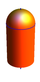
The geometry we want to consider in this analysis is a $(2+1)$-dimensional spacetime corresponding to a semi-cylindrical surface with topology $S^{1}\times R^{1}$, capped by a hemisphere (see figure 1). The coordinates covering all the manifold will be denoted by $(x^{0}=t,x^{1},x^{2})$, where $0\leqslant x^{2}\leqslant L$, being $L$ the length of the compact dimension in the semi-cylinder subspace. The definition of $x^{1}$ is in according with the submanifold. The metric tensor associated with each subspace is specified by the following line elements:

• For the hemisphere we have

  $$ds^{2}=dt^{2}-(dx^{1})^{2}-\sin^{2}(x^{1}/a)(dx^{2})^{2},$$ (2.1)

  where $0\leqslant x^{1}\leqslant\pi a/2$, with $a=L/(2\pi)$ being the radius.

• For the semi-cylinder we have

  $$ds^{2}=dt^{2}-(dx^{1})^{2}-(dx^{2})^{2},$$ (2.2)

  where $\pi a/2\leqslant x^{1}<\infty$.

Note that the coordinate $x^{1}$ measures the distance from the top of the hemisphere.

Figure 1: Cylindrical tube with a hemisphere cap.

In addition to the spatial coordinates $(x^{1},x^{2})$ we shall use the angular coordinates $(\theta,\phi)$ defined as

$$\theta=x^{1}/a,\;\phi=x^{2}/a,\;0\leqslant\phi\leqslant 2\pi.$$ (2.3)

The angle $\phi$ is the standard azimuthal one with the range $[0,2\pi]$; as to $\theta$ it is the usual polar angle on the hemisphere, on which $0\leqslant\theta\leqslant\pi/2$ and $\theta=0$ corresponds to the top of the hemisphere. On the semi-cylinder its range is $\pi/2\leqslant\theta<\infty$. The circle $\theta=\pi/2$ corresponds to the boundary between the two geometries (2.1) and (2.2) (circle in figure 1). In the coordinates $(t,\theta,\phi)$ the metric tensor is given by the expressions:

$$g_{ik}=\left\{\begin{array}[]{ll}\mathrm{diag}(1,-a^{2},-a^{2}\sin^{2}\theta),&0\leqslant\theta\leqslant\pi/2,\\ \mathrm{diag}(1,-a^{2},-a^{2}),&\pi/2\leqslant\theta<\infty.\end{array}\right.$$ (2.4)

The metric tensor and its first derivatives are continuous at $\theta=\pi/2$. So there is no need to introduce an additional ”surface” energy-momentum tensor located on the boundary. In the region $0\leqslant\theta<\pi/2$, for the components of the Ricci tensor and for the curvature scalar one has

$$R_{0}^{0}=0,\;R_{i}^{k}=a^{-2}\delta_{i}^{k},\;R=2a^{-2},\;i,k=1,2.$$ (2.5)

In the region $\pi/2<\theta<\infty$ the spacetime is flat. Note that the extrinsic curvature tensor vanishes for both sides of the boundary.

Let us consider a massive quantum scalar field, $\varphi(x)$, with an arbitrary curvature coupling parameter, $\xi$, on background of the geometry described by the metric tensor (2.4). The corresponding equation of motion reads

$$(g^{ik}\nabla_{i}\nabla_{k}+m^{2}+\xi R)\varphi(x)=0.$$ (2.6)

The most important special cases correspond to minimally ($\xi=0$) and conformally ($\xi=1/8$) coupled fields. The hemisphere cap will change the properties of the scalar vacuum on the cylindrical part of the space compared with the case of an infinite tube. Similarly, the cylindrical geometry will induce changes in the VEVs of physical observables on the hemisphere, when compared to the case of the spherical geometry $S^{2}$. These changes can be referred as geometrically induced Casimir densities. In the problem under consideration, the only interaction of the field is with the background geometry and all the properties of the quantum vacuum may be deduced from two-point functions. Here we will evaluate the positive-frequency Wightman function. The consideration of other two-point functions is similar. For the evaluation of the Wightman function we shall follow the direct mode-summation approach. In this approach a complete set of normalized mode functions, $\{\varphi_{\sigma}(x),\varphi_{\sigma}^{\ast}(x)\}$, is required. Here we have denoted by $\sigma$ the set of quantum numbers specifying the mode functions.

In accordance with the symmetry of the problem, the mode functions can be presented in the factorized form as,

$$\varphi_{\alpha}(x)=f(\theta)e^{in\phi-i\omega t},\;n=0,\pm 1,\pm 2,\ldots$$ (2.7)

Substituting this expression into (2.6) we get the equation for the function $f(\theta)$. In the cylindrical part, the solution of the equation is given by

$$f(\theta)=C_{\mathrm{c}}\cos[p\left(\theta-\pi/2\right)-\alpha],$$ (2.8)

with constants $C_{\mathrm{c}}$ and $\alpha$, and

$$p=\sqrt{\omega^{2}a^{2}-n^{2}-m^{2}a^{2}}.$$ (2.9)

Here we assume that $p\geqslant 0$ . The allowance of bound states with purely imaginary $p$ will be discussed below.

On the hemisphere, the equation for the function $f(\theta)$ reads

$$\left[\frac{1}{\sin\theta}\partial_{\theta}\left(\sin\theta\partial_{\theta}\right)-\frac{n^{2}}{\sin^{2}\theta}+\omega^{2}a^{2}-m^{2}a^{2}-2\xi\right]f(\theta)=0.$$ (2.10)

The solution of this equation, regular at $\theta=0$, is given in terms of the associated Legendre function of the first kind (for the properties of the associated Legendre functions $P_{\nu}^{\mu}(x)$ and $Q_{\nu}^{\mu}(x)$ on the cut $-1<x<1$ see [25]):

$$f(\theta)=C_{\mathrm{s}}P_{\lambda-1/2}^{-|n|}(u),\;u=\cos\theta,$$ (2.11)

where

$$\lambda=\sqrt{\omega^{2}a^{2}-\omega_{m}^{2}}.$$ (2.12)

with the notation

$$\omega_{m}=\sqrt{m^{2}a^{2}+2\xi-1/4}.$$ (2.13)

Note that, because of the property $P_{-\lambda-1/2}^{-|n|}(u)=P_{\lambda-1/2}^{-|n|}(u)$, the both signs of the square root in (2.12) lead to the same solution.

The solutions (2.8) and (2.11) contain three constants. One of them is determined by the normalization condition and the remaining two are determined from the matching conditions for the field and for its normal derivative at $\theta=\pi/2$. In the problem under consideration the derivatives of the metric tensor are continuous at the boundary and, hence, the Ricci scalar in (2.6) does not contain delta function terms. As a consequence of this, both the field $\varphi(x)$ and its derivative $\partial_{\theta}\varphi(x)$ are continuous at $\theta=\pi/2$. From these conditions we get

$$e^{-2i\alpha}=\frac{pP_{\lambda-1/2}^{-|n|}+iP_{\lambda-1/2}^{-|n|\prime}}{pP_{\lambda-1/2}^{-|n|}-iP_{\lambda-1/2}^{-|n|\prime}},$$ (2.14)

for the phase in (2.8), and the relation

$$C_{\mathrm{s}}=\frac{pC_{\mathrm{c}}}{\sqrt{(pP_{\lambda-1/2}^{-|n|})^{2}+(P_{\lambda-1/2}^{-|n|\prime})^{2}}},$$ (2.15)

for the normalization coefficients. In these expressions we have introduced the notations

$$P_{\lambda-1/2}^{-|n|}=P_{\lambda-1/2}^{-|n|}(0),\;P_{\lambda-1/2}^{-|n|\prime}=\partial_{u}P_{\lambda-1/2}^{-|n|}(u)|_{u=0}.$$ (2.16)

The expressions for $P_{\lambda-1/2}^{-|n|}$ and $P_{\lambda-1/2}^{-|n|\prime}$ in terms of the gamma function are given in [25]. By using the formula $\sin(\pi z)\Gamma(z)=\pi/\Gamma(1-z)$ we get simpler representations:

$$P_{\lambda-1/2}^{-|n|} = \frac{2^{-|n|}\sqrt{\pi}}{\Gamma\left(\left(|n|+\lambda+3/2\right)/2\right)\Gamma(\left(|n|-\lambda+3/2\right)/2)},$$

$$P_{\lambda-1/2}^{-|n|\prime} = -\frac{2^{1-|n|}\sqrt{\pi}}{\Gamma\left(\left(|n|+\lambda+1/2\right)/2\right)\Gamma(\left(|n|-\lambda+1/2\right)/2)}.$$ (2.17)

So, the mode functions (2.8) and (2.11) are specified by the set of quantum numbers $\sigma=(p,n)$.

The constant $C_{\mathrm{c}}$ is determined by the normalization condition

$$\int_{0}^{\infty}d\theta\int_{0}^{2\pi}d\phi\sqrt{|g|}\varphi_{\sigma}(x)\varphi_{\sigma^{\prime}}^{\ast}(x)=\frac{\delta_{nn^{\prime}}}{2\omega}\delta(p-p^{\prime}).$$ (2.18)

For $p^{\prime}=p$ the integral over $\theta$ is divergent and the dominant contribution comes from the large values of $\theta$. In this case, in order to determine $C_{\mathrm{c}}$, it is sufficient to consider the part in the integral over the cylindrical geometry, $\theta>\pi/2$. In this way we find

$$|C_{\mathrm{c}}|^{2}=\frac{1}{2\pi^{2}a^{2}\omega}.$$ (2.19)

Now, the mode functions with the continuous energy spectrum are written as

$$\varphi_{\sigma}(x) = C_{\mathrm{s}}P_{\lambda-1/2}^{-|n|}(\cos\theta)e^{in\phi-i\omega t},\;0\leqslant\theta\leqslant\pi/2,$$ (2.20)

$$\varphi_{\sigma}(x) = C_{\mathrm{c}}\cos[p\left(\theta-\pi/2\right)-\alpha]e^{in\phi-i\omega t},\;\pi/2\leqslant\theta<\infty,$$ (2.21)

where $0\leqslant p<\infty$ and $C_{\mathrm{s}}$ is given by (2.15).

We can have also bound states for which $p$ is pure imaginary, $p=i\eta$ with $\eta>0$. From the stability of the vacuum one has $\omega^{2}\geqslant 0$ and from (2.9) we obtain $\eta\leqslant ma$. For the bound states the solution in the part of the cylindrical geometry has the form

$$\varphi_{\mathrm{b}\sigma}(x)=C_{\mathrm{bc}}e^{-\eta\theta+in\phi-i\omega t}.$$ (2.22)

On the cup the corresponding solution is given by (2.20) with $C_{\mathrm{s}}$ replaced by a new constant $C_{\mathrm{bs}}$. From the continuity of the mode functions and their first derivatives at $\theta=\pi/2$ one gets the equation

$$P_{\lambda-1/2}^{-|n|\prime}-\eta P_{\lambda-1/2}^{-|n|}=0,$$ (2.23)

where

$$\lambda=\sqrt{n^{2}-\eta^{2}-2\xi+1/4}.$$ (2.24)

Now, by using the relation

$$P_{\lambda-1/2}^{-|n|\prime}=\frac{-1/P_{\lambda-1/2}^{-|n|}}{\Gamma(|n|+\lambda+1/2)\Gamma(|n|-\lambda+1/2)},$$ (2.25)

which directly follows from (2.17), the equation for the bound states is rewritten as

$$\frac{1}{\Gamma(|n|+\lambda+1/2)\Gamma(|n|-\lambda+1/2)}+\eta(P_{\lambda-1/2}^{-|n|})^{2}=0.$$ (2.26)

For purely imaginary $\lambda$ the lhs of the above expression is always positive and we conclude that in this case there are no bound states. The same is true in the case $0\leqslant\lambda\leqslant|n|+1/2$. Hence, the bound states may be present in the case $\lambda>|n|+1/2$ only. Combining this with (2.24), we conclude that the bound states may exist under the condition $\xi<-|n|/2$ only. In particular, there are no bound states for minimally and conformally coupled fields. In what follows we assume that $\xi\geqslant 0$ and, hence, the bound states are absent.

3 Two-point function

Having the complete set of normalized mode functions (2.20) and (2.21), we can evaluate any of two-point functions for a scalar field. In particular, for the positive frequency Wightman function one has the mode-sum formula

$$W(x,x^{\prime})=\sum_{n=-\infty}^{+\infty}\int_{0}^{\infty}dp\,\varphi_{\sigma}(x)\varphi_{\sigma}^{\ast}(x^{\prime}).$$ (3.1)

First we consider the region $\pi/2<\theta<\infty$ corresponding to the part of the space with cylindrical geometry.

3.1 Cylindrical geometry

Substituting the corresponding mode functions from (2.21) into (3.1) and using the expression for $\alpha$, given by (2.14), the Wightman function is presented in the form

$$W(x,x^{\prime}) = W_{0}(x,x^{\prime})+\frac{1}{L^{2}}\sideset{}{{}^{\prime}}{\sum}_{n=0}^{\infty}\cos(n\Delta\phi)\int_{0}^{\infty}dp$$ (3.2)

$$\times\frac{e^{-i\omega\Delta t}}{\omega}\sum_{s=\pm 1}e^{sip(\theta+\theta^{\prime}-\pi)}\frac{pP_{\lambda-1/2}^{-n}+siP_{\lambda-1/2}^{-n\prime}}{pP_{\lambda-1/2}^{-n}-siP_{\lambda-1/2}^{-n\prime}},$$

where $\Delta\phi=\phi-\phi^{\prime}$, $\Delta t=t-t^{\prime}$, $\omega$ is expressed in terms of $p$ by using (2.9), and the prime on the sign of the sum means that the term $n=0$ should be taken with the coefficient 1/2. In (3.2),

$$W_{0}(x,x^{\prime})=\frac{2}{L^{2}}\sideset{}{{}^{\prime}}{\sum}_{n=0}^{\infty}\cos(n\Delta\phi)\int_{0}^{\infty}dp\,\cos(p\Delta\theta)\frac{e^{-i\omega\Delta t}}{\omega},$$ (3.3)

with $\Delta\theta=\theta-\theta^{\prime}$, is the Wightman function for an infinite tube described by the line element (2.2) for $-\infty<\theta<+\infty$. By using the Abel-Plana summation formula (see, for instance, [16, 26]) for the series over $n$ in (3.3), this function can be presented in the form

$$W_{0}(x,x^{\prime})=\frac{1}{4\pi a}\sum_{l=-\infty}^{\infty}\frac{e^{-ma\sqrt{(\Delta\theta)^{2}+\left(\Delta\phi+2\pi l\right)^{2}-(\Delta t/a)^{2}}}}{\sqrt{(\Delta\theta)^{2}+\left(\Delta\phi+2\pi l\right)^{2}-(\Delta t/a)^{2}}}.$$ (3.4)

In this representation, the $l=0$ term is the Wightman function for Minkowski spacetime with spatial topology $R^{2}$. The formula (3.4) presents the Wightman function for an infinite tube as an image sum of the Minkowskian functions.

The second term in the rhs of (3.2) is induced by the hemisphere cap. For the further transformation of this part, under the condition $\theta+\theta^{\prime}>\pi+\Delta t/a$, we rotate the integration contour over $p$ by the angle $\pi/2$ for the term with $s=+1$ and by the angle $-\pi/2$ for the term with $s=-1$. The integrals over the intervals $(0,ima)$ and $(0,-ima)$ cancel out and, after some transformations, one finds

$$W(x,x^{\prime}) = W_{0}(x,x^{\prime})+\frac{1}{2\pi^{2}a}\sideset{}{{}^{\prime}}{\sum}_{n=0}^{\infty}\cos(n\Delta\phi)\int_{ma}^{\infty}dy\,y$$ (3.5)

$$\times\frac{\cosh(\sqrt{y^{2}-m^{2}a^{2}}\Delta t/a)}{\sqrt{y^{2}-m^{2}a^{2}}}\frac{e^{-\sqrt{y^{2}+n^{2}}(\theta+\theta^{\prime}-\pi)}}{\sqrt{y^{2}+n^{2}}}f_{n}(y).$$

Here we have introduced the notation

$$f_{n}(y)=\frac{\sqrt{y^{2}+n^{2}}P_{iz(y)-1/2}^{-n}+P_{iz(y)-1/2}^{-n\prime}}{\sqrt{y^{2}+n^{2}}P_{iz(y)-1/2}^{-n}-P_{iz(y)-1/2}^{-n\prime}},$$ (3.6)

with

$$z(y)=\sqrt{y^{2}+2\xi-1/4}.$$ (3.7)

Note that the function $z(y)$ can be either real or purely imaginary. In both cases the function $P_{iz(y)-1/2}^{-n}$ is real. For $\xi\geqslant 0$ the function in the denominator of (3.6) is positive. Unlike to the oscillating integrand in (3.2), the integrand in (3.5), under the condition mentioned above, is exponentially decreasing near the upper limit of the integration and the representation (3.5) is well adapted for the evaluation of the VEVs in the coincidence limit.

3.2 Hemisphere cap

In this subsection we consider the two-point function on the hemispherical cap (for the zeta function and heat kernel coefficients on Riemann caps see [27]). From the mode-sum formula (3.1) with the mode functions from (2.20), for the Wightman function on the hemisphere cap, one has

$$W(x,x^{\prime})=\frac{4}{L^{2}}\sideset{}{{}^{\prime}}{\sum}_{n=0}^{\infty}\cos(n\Delta\phi)\int_{0}^{\infty}dp\,p^{2}\frac{P_{\lambda-1/2}^{-n}(\cos\theta)P_{\lambda-1/2}^{-n}(\cos\theta^{\prime})}{(pP_{\lambda-1/2}^{-n})^{2}+(P_{\lambda-1/2}^{-n\prime})^{2}}\frac{e^{-i\omega\Delta t}}{\omega},$$ (3.8)

with $0\leqslant\theta,\theta^{\prime}<\pi/2$ and $\lambda$ is given by (2.12). Our interest in this paper is the effects on the sphere, induced by the cylindrical geometry, in the region $\theta>\pi/2$. In order to explicitly extract from (3.8) the part induced by this geometry, we note that the denominator in the integrand of (3.8) is equal to $\bar{P}_{\lambda-1/2}^{+,-|n|}(0)\bar{P}_{\lambda-1/2}^{-,-|n|}(0)$, where the notations with bars are defined by the relation (A.3) in the appendix A. By using the identity (A.8) with $\theta=\pi/2$, the function (3.8) is expressed as

$$W(x,x^{\prime}) = \frac{i}{L^{2}}\sideset{}{{}^{\prime}}{\sum}_{n=0}^{\infty}(-1)^{n}\cos(n\Delta\phi)\int_{0}^{\infty}dp\,p\frac{e^{-i\omega\Delta t}}{\omega}$$ (3.9)

$$\times P_{\lambda-1/2}^{-n}(\cos\theta)P_{\lambda-1/2}^{n}(\cos\theta^{\prime})\sum_{j=+,-}j\frac{\bar{S}_{\lambda-1/2}^{j,-n}(0)}{\bar{P}_{\lambda-1/2}^{j,-n}(0)},$$

where the functions $\bar{S}_{\lambda-1/2}^{j,-n}(x)$ are defined by the expressions (A.9) and (A.10) in appendix A and we have used the relation [25]

$$P_{\lambda-1/2}^{-n}(u)=(-1)^{n}\frac{\Gamma\left(\lambda-n+1/2\right)}{\Gamma\left(\lambda+n+1/2\right)}P_{\lambda-1/2}^{n}(u).$$ (3.10)

Note that the integrand in (3.9) is an even function of $\lambda$.

The expressions for $S_{\lambda-1/2}^{-n}(0)$ and $S_{\lambda-1/2}^{-n\prime}(0)$, entering in (3.9), in terms of the gamma function are found by using the corresponding expressions for $Q_{\lambda-1/2}^{-n}(0)$ and $Q_{\lambda-1/2}^{-n\prime}(0)$ from [25]. The latter can be written as

$$Q_{\lambda-1/2}^{-n}(0) = -\frac{\pi}{2}\tan\left[\pi(\lambda-n-1/2)/2\right]P_{\lambda-1/2}^{-n},$$

$$Q_{\lambda-1/2}^{-n\prime}(0) = \frac{\pi}{2}\cot\left[\pi(\lambda-n-1/2)/2\right]P_{\lambda-1/2}^{-n\prime},$$ (3.11)

with $P_{\lambda-1/2}^{-n}$ and $P_{\lambda-1/2}^{-n\prime}$ given in (2.17). By using these relations, we can see that

$$S_{\lambda-1/2}^{-n}(0) = \pi(-1)^{n}\frac{P_{\lambda-1/2}^{-n}}{\cos(\pi\lambda)},$$

$$S_{\lambda-1/2}^{-n\prime}(0) = -\pi(-1)^{n}\frac{P_{\lambda-1/2}^{-n\prime}}{\cos(\pi\lambda)}.$$ (3.12)

By taking into account that in the complex plane $p$ and under the condition $\pi-\theta-\theta^{\prime}-\Delta t/a>0$, the integrand of (3.9) exponentially decreases for $|\mathrm{Im}\,p|\rightarrow\infty$, we rotate the integration contour over $p$ by the angle $\pi/2$ ($-\pi/2$) for the term with $j=+$ ($j=-$). Note that, though the integrand in (3.9) has no poles on the real axis, this is not the case for separate terms in the sum over $j$. By taking into account the relation (A.11), we see that the separate terms have poles at the zeros of the function $\cos(\lambda\pi)$. In the integral over $p$ we will shift the integration contour by a small amount $\epsilon>0$ assuming that the integration goes over the half-line $[0-i\epsilon,\infty-i\epsilon)$. Now, in the rotation for the $j=+$ term, we note that the integrand has poles at the zeros of the function $\cos(\lambda\pi)$ and the corresponding residues should be included. After the rotation of the contours, the integrals over the regions $(0,i\sqrt{n^{2}+m^{2}a^{2}})$ and $(0,-i\sqrt{n^{2}+m^{2}a^{2}})$ cancel out. In this way, by using the relations (3.12), from (3.9) one gets

$$W(x,x^{\prime}) = W_{S^{2}}(x,x^{\prime})-\frac{1}{L}\sideset{}{{}^{\prime}}{\sum}_{n=0}^{\infty}\cos(n\Delta\phi)\int_{ma}^{\infty}dy\,\frac{yf_{n}(y)}{\cosh(\pi z(y))}$$ (3.13)

$$\times P_{iz(y)-1/2}^{-n}(\cos\theta)P_{iz(y)-1/2}^{n}(\cos\theta^{\prime})\frac{\cosh(\sqrt{y^{2}-m^{2}a^{2}}\Delta t/a)}{\sqrt{y^{2}-m^{2}a^{2}}},$$

where the functions $f_{n}(y)$ and $z(y)$ were already defined by the relations (3.6) and (3.7). The first term in the rhs of (3.13) comes from the residues at the zeros of the function $\cos(\lambda\pi)$ and coincides with the Wightman function for a scalar field on the sphere $S^{2}$ (see the appendix B). After the summation over $n$ by using the formula [25]

$$\sum_{n=-l}^{+l}(-1)^{|n|}P_{l}^{-|n|}(\cos\theta)P_{l}^{|n|}(\cos\theta^{\prime})e^{in\Delta\phi}=P_{l}(\cos\gamma),$$ (3.14)

this function is expressed as

$$W_{S^{2}}(x,x^{\prime})=\frac{a^{-2}}{8\pi}\sum_{l=0}^{\infty}\frac{2l+1}{\omega_{l}}e^{-i\omega_{l}\Delta t}P_{l}(\cos\gamma).$$ (3.15)

In this formula, $P_{l}(z)$ is the Legendre polynomial and

$$\omega_{l} = a^{-1}\sqrt{l(l+1)+m^{2}a^{2}+2\xi},$$

$$\cos\gamma = \cos\theta\cos\theta^{\prime}+\sin\theta\sin\theta^{\prime}\cos(\Delta\phi).$$ (3.16)

When compared with (3.9), the representation (3.13) has two important advantages. First of all, the part describing the effects induced by the cylindrical tube is explicitly extracted. In this way, for points away from the boundary $\theta=\pi/2$, the renormalization of the VEVs in the coincidence limit is reduced to the one for the geometry $S^{2}$. And second, under the condition $\pi-\theta-\theta^{\prime}-\Delta t/a>0$, the integrand in the tube-induced part of (3.13) exponentially decreases near the upper limit of the integration. This is important in the numerical evaluation of the local VEVs in the coincidence limit.

4 Mean field squared

Formally the VEV of the field squared is obtained from the Wightman function by taking the coincidence limit of the arguments. However, this procedure results in a divergent quantity and some renormalization procedure is needed to provide a well defined finite value. We shall consider the cylindrical and hemisphere parts separately.

Let us start with the part of the geometry corresponding to the cylindrical tube. In this subspace the spacetime is flat and the renormalization is reduced to the subtraction from the VEVs the corresponding VEVs in $(2+1)$-dimensional Minkowski spacetime with trivial topology. The latter is given by the $l=0$ term in (3.4). Omitting this term and using the expression (3.5) for the Wightman function, the renormalized VEV of the field squared is expressed in the form

$$\langle\varphi^{2}\rangle = \langle\varphi^{2}\rangle_{0}+\frac{1}{\pi L}\sideset{}{{}^{\prime}}{\sum}_{n=0}^{\infty}\int_{ma}^{\infty}dy\,$$ (4.1)

$$\times\frac{yf_{n}(y)}{\sqrt{y^{2}-m^{2}a^{2}}}\frac{e^{-\sqrt{y^{2}+n^{2}}(2\theta-\pi)}}{\sqrt{y^{2}+n^{2}}},$$

for $\theta>\pi/2$. Here

$$\langle\varphi^{2}\rangle_{0}=-\frac{1}{2\pi L}\ln(1-e^{-Lm}),$$ (4.2)

is the VEV for an infinite tube and the second term in the rhs is induced by the cap. Note that for a massless field the VEV contains infrared divergences.

For large values of $n$ and $y$, by using the asymptotic formula for the gamma function for large values of the argument, we can see that to the leading order

$$f_{n}(y)\approx\frac{(y^{2}+n^{2})\left(1-4\xi\right)-n^{2}}{8(y^{2}+n^{2})^{2}}.$$ (4.3)

From here it follows that the cap-induced part in (4.1) is finite for all values of $\pi/2\leqslant\theta<\infty$, including the points on the boundary $\theta=\pi/2$. At large distances from the tube edge, $a(\theta-\pi/2)\gg 1/m$, the dominant contribution to the integral in (4.1) comes from the region near the lower limit and to the leading order we get

$$\langle\varphi^{2}\rangle\approx\langle\varphi^{2}\rangle_{0}+\frac{f_{0}(ma)e^{-ma(2\theta-\pi)}}{4L\sqrt{\pi ma(\theta-\pi/2)}}.$$ (4.4)

In this limit the cap-induced contribution is exponentially small. The expression (4.4) describes also the behavior of the cap-induced part in the limit of large values for the tube radius with fixed value of $\theta-\pi/2$. Note that in this limit one has $\langle\varphi^{2}\rangle_{0}\approx e^{-Lm}/(2\pi L)$ and for $\theta<3\pi/2$ the total VEV is dominated by the cap-induced contribution.

It will be interesting to compare the expressions for the hemisphere capped tube with the corresponding results for a semi-infinite (si) tube with Dirichlet or Neumann boundary conditions at the edge $\theta=\pi/2$. The Wightman function and the VEV of the field squared in the latter geometry are obtained from (3.5) and (4.1) by the replacement $f_{n}(y)\rightarrow\mp 1$, where the upper and lower signs correspond to Dirichlet and Neumann boundary conditions, respectively. With this replacement, after the integration over $y$, we get

$$\langle\varphi^{2}\rangle_{\mathrm{si}}=\langle\varphi^{2}\rangle_{0}\mp\frac{1}{\pi L}\sideset{}{{}^{\prime}}{\sum}_{n=0}^{\infty}K_{0}((2\theta-\pi)\sqrt{n^{2}+m^{2}a^{2}}),$$ (4.5)

where $K_{\nu}(x)$ is the MacDonald function. The second term in the rhs of (4.5) is induced by the edge of the tube. For Neumann boundary condition the VEV (4.5) is positive, whereas for Dirichlet boundary condition it is negative near the edge and positive at large distances. For points close to the boundary, the contribution of large $n$ dominates in (4.5) and, to the leading order, the summation can be replaced by the integration. In this way, we see that for a semi-infinite tube with Dirichlet or Neumann boundary conditions the VEV of the field squared diverges on the boundary as $1/(2\theta-\pi)$.

In the part of the geometry corresponding to the hemisphere cap we use the expression (3.13) for the Wightman function. In the coincidence limit this gives

$$\langle\varphi^{2}\rangle=\langle\varphi^{2}\rangle_{S^{2}}-\frac{1}{L}\sideset{}{{}^{\prime}}{\sum}_{n=0}^{\infty}\int_{ma}^{\infty}dy\,\frac{yg_{n}(y)}{\sqrt{y^{2}-m^{2}a^{2}}}\frac{[P_{iz(y)-1/2}^{-n}(\cos\theta)]^{2}}{\cosh[\pi z(y)]},$$ (4.6)

where $\theta<\pi/2$ and we have introduced the notation

$$g_{n}(y) = (-1)^{n}\frac{\Gamma(iz(y)+n+1/2)}{\Gamma(iz(y)-n+1/2)}f_{n}(y)$$ (4.7)

$$= \frac{\sqrt{y^{2}+n^{2}}P_{iz(y)-1/2}^{n}+P_{iz(y)-1/2}^{n\prime}}{\sqrt{y^{2}+n^{2}}P_{iz(y)-1/2}^{-n}-P_{iz(y)-1/2}^{-n\prime}}.$$

The renormalization is reduced to that for the first term in the rhs, corresponding to the geometry $S^{2}$. The expression for the renormalized $\langle\varphi^{2}\rangle_{S^{2}}$ is derived in the appendix B. The second term in the rhs of (4.6) is induced by the cylindrical tube. For large values of $y$ the function $P_{iz(y)-1/2}^{-n}(\cos\theta)$ behaves as $e^{y\theta}$, and the integrand in (4.6) decays as $e^{-y(2\theta-\pi)}$ for $\theta<\pi/2$. By taking into account the asymptotic expression (4.3), we see that the tube-induced part is finite at the boundary, $\theta=\pi/2$.

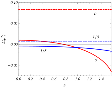
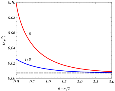
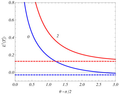
In figure 2 we have plotted the renormalized mean field squared as a function of $\theta$ in hemispherical (left panel) and cylindrical (right panel) regions for minimally and conformally coupled field (the numbers near the curves are the values of the curvature coupling parameter $\xi$). The graphs are plotted for $ma=1/2$. The dashed curves present the renormalized VEV of the field squared on $S^{2}$ (left panel) and on an infinite tube (right panel). In the cylindrical part, the VEV $\langle\varphi^{2}\rangle_{0}$ does not depend on the curvature coupling. On the hemispherical cap, the tube-induced contribution in the VEV of the field squared is negative for both the minimal and conformal couplings, whereas on the tube the cap-induced parts are positive.

Figure 2: Renormalized VEV of the field squared on the hemisphere cap (left panel) and on the cylindrical tube (right panel) for minimally and conformally coupled scalar fields. The numbers near the curves are the values of the curvature coupling parameter $\xi$ and the graphs are plotted for $ma=1/2$. The dashed curves display the renormalized VEVs on $S^{2}$ (left panel) and on an infinite tube (right panel).

As is seen from fig 2, though the Wightman function is continuous at the boundary, the renormalized VEV of the field squared is not continuous. The reason for this is that in the renormalization procedure for separate regions of tube and hemisphere we have subtracted different terms. In the tube part of the geometry the subtracted term coincides with the corresponding VEV in Minkowski spacetime, whereas on the hemisphere, in addition to the Minkowskian term, we have also subtracted a finite renormalization term $(1/6-\xi)/(4\pi ma^{2})$. We have numerically checked that the VEV evaluated by the minimal subtraction scheme (on the hemisphere the Minkowskian part is subtracted only), $\langle\varphi^{2}\rangle_{\mathrm{min}}=\langle\varphi^{2}\rangle+(1/6-\xi)/(4\pi ma^{2})$, is continuous on the boundary.

5 Energy-momentum tensor and the Casimir force

In this section, we shall study the vacuum energy-momentum tensor and the Casimir force for the system under consideration. Given the Wightman function and the VEV of the field squared, the VEV of the energy-momentum tensor is evaluated by using the formula

$$\langle T_{ik}\rangle=\lim_{x^{\prime}\rightarrow x}\partial_{i^{\prime}}\partial_{k}W(x,x^{\prime})+\left[\left(\xi-1/4\right)g_{ik}\nabla_{p}\nabla^{p}-\xi\nabla_{i}\nabla_{k}-\xi R_{ik}\right]\langle\varphi^{2}\rangle,$$ (5.1)

where $R_{ik}$ is the Ricci tensor. In the rhs of this formula we have used the expression for the energy-momentum tensor of a scalar filed which differs from the standard expression [28] by the term which does not contribute to the VEVs (see [29]).

5.1 Casimir densities on the tube

On the tube, $\pi/2<\theta<\infty$, the off-diagonal components of the vacuum energy-momentum tensor vanish and the diagonal components are decomposed as (with no summation over $l$)

$$\langle T_{l}^{l}\rangle=\langle T_{l}^{l}\rangle_{0}-\frac{a^{-3}}{2\pi^{2}}\sideset{}{{}^{\prime}}{\sum}_{n=0}^{\infty}\int_{ma}^{\infty}dy\,\frac{yf_{n}(y)}{\sqrt{y^{2}-m^{2}a^{2}}}\frac{e^{-\sqrt{y^{2}+n^{2}}(2\theta-\pi)}}{\sqrt{y^{2}+n^{2}}}F_{n}^{(l)}(y),$$ (5.2)

where the first term in the rhs corresponds to the geometry of an infinite tube and the second term is induced by the hemisphere cap. For the functions in the latter one has $F_{n}^{(1)}(y)=0$ and

$$F_{n}^{(0)}(y) = 4\xi\left(y^{2}+n^{2}\right)-n^{2}-m^{2}a^{2},$$

$$F_{n}^{(2)}(y) = \left(4\xi-1\right)\left(y^{2}+n^{2}\right)+n^{2}.$$ (5.3)

Hence, the cap-induced contribution to the vacuum stress normal to the boundary vanishes on the tube. This result could be obtained by general arguments, based on the covariant conservation equation $\nabla_{k}\langle T_{i}^{k}\rangle=0$. From the symmetry of the problem it follows that the cap-induced part depend only on the coordinate $\theta$ and this equation is reduced to a single constraint $\partial_{\theta}\langle T_{1}^{1}\rangle_{\mathrm{c}}=0$, where $\langle T_{1}^{1}\rangle_{\mathrm{c}}$ is the cap-induced part (second term in the rhs of (5.2)). Now, from the condition $\langle T_{1}^{1}\rangle_{\mathrm{c}}\rightarrow 0$ for $\theta\rightarrow\infty$ it follows that $\langle T_{1}^{1}\rangle_{\mathrm{c}}=0$.

The part of the VEV corresponding to an infinite tube does not depend on the curvature coupling parameter and is expressed as (no summation over $l$):

$$\langle T_{l}^{l}\rangle_{0}=\frac{F^{(l)}(mL)}{2\pi L^{3}},$$ (5.4)

where we have introduced the notations

$$F^{(0)}(x) = F^{(1)}(x)=-\mathrm{Li}_{3}(e^{-x})-x\,\mathrm{Li}_{2}(e^{-x}),$$

$$F^{(2)}(x) = 2\mathrm{Li}_{3}(e^{-x})+2x\,\mathrm{Li}_{2}(e^{-x})-x^{2}\ln(1-e^{-x}),$$ (5.5)

with $\mathrm{Li}_{j}(x)=\sum_{n=1}^{\infty}x^{n}/n^{j}$ being the polylogarithm function. For a massless field one has (for the Casimir effect in topologically nontrivial three-dimensional spacetimes see [16])

$$\langle T_{0}^{0}\rangle_{0}=\langle T_{1}^{1}\rangle_{0}=-\frac{1}{2}\langle T_{2}^{2}\rangle_{0}=-\frac{\zeta(3)}{2\pi L^{3}},$$ (5.6)

where $\zeta(s)$ is the Riemann zeta function. For a massive field and for large values of the tube radius, $mL\gg 1$, to the leading order we get

$$\langle T_{0}^{0}\rangle_{0}\approx\frac{-1}{mL}\langle T_{2}^{2}\rangle_{0}\approx-\frac{me^{-Lm}}{2\pi L^{2}}\,.$$ (5.7)

As an additional check we can see that both the cylindrical and cap-induced parts obey the trace relation

$$\langle T_{l}^{l}\rangle=2\left(\xi-1/8\right)\nabla_{l}\nabla^{l}\langle\varphi^{2}\rangle+m^{2}\langle\varphi^{2}\rangle.$$ (5.8)

Unlike to the VEV of the field squared, the energy density and the stress $\langle T_{2}^{2}\rangle$ in (5.2) diverge on the boundary $\theta=\pi/2$. These divergences come from the cap-induced part. In order to find the leading terms in the corresponding asymptotic expansions, we note that for points near the boundary the dominant contribution to the cap-induced part in (5.2) comes from large values of $n$ and $y$. By taking into account (4.3), to the leading order we get (no summation over $l$)

$$\langle T_{l}^{l}\rangle\approx\frac{2\xi\left(4\xi-1\right)+(l+1)/16}{16\pi(2\theta-\pi)a^{3}},$$ (5.9)

with $l=0,2$. For both minimally and conformally coupled fields the parallel stress is positive near the boundary, whereas the energy density is positive for a minimally coupled field and negative for the conformal coupling.

At large distances from the edge of the tube and for a massive field, $a(\theta-\pi/2)\gg 1/m$, the dominant contribution to the cap-induced part in (5.2) comes from the term $n=0$ and from the region of the integration near the lower limit. To the leading order we find (no summation over $l=0,2$)

$$\langle T_{l}^{l}\rangle\approx\langle T_{l}^{l}\rangle_{0}-\frac{4\xi-1}{4\pi^{2}a^{3}}\frac{(ma)^{3/2}f_{0}(ma)}{\sqrt{2(2\theta/\pi-1)}}e^{-ma(2\theta-\pi)},$$ (5.10)

and the VEV is exponentially small. For a massless field, at large distances, $\theta-\pi/2\gg 1$, one has a power-law decay (no summation over $l=0,2$):

$$\langle T_{l}^{l}\rangle\approx\langle T_{l}^{l}\rangle_{0}+\frac{a^{-3}}{4\pi^{2}}\frac{4\xi-\delta_{l}^{2}}{(2\theta-\pi)^{2}}.$$ (5.11)

For a semi-infinite tube with Dirichlet or Neumann boundary conditions on its edge, $\theta=\pi/2$, the VEV of the energy-momentum tensor is obtained from (5.2) with the replacement $f_{n}(y)\rightarrow\mp 1$, where the upper and lower signs are for Dirichlet and Neumann conditions, respectively. In this case, the integral over $y$ is expressed in terms of the MacDonald functions $K_{0}(x)$ and $K_{1}(x)$ with the same argument as in (4.5). Near the boundary and for non-conformally coupled fields the leading terms in the energy density and the parallel stress behave like $1/(2\theta-\pi)^{3}$. As we see, the divergences here are stronger than those in the problem under consideration.

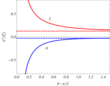
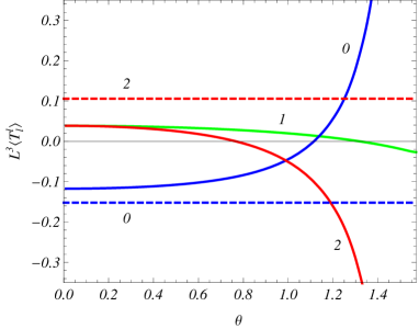
In figure 3 we have displayed the components of the vacuum energy-momentum tensor on the tube as functions of the distance from the boundary $\theta=\pi/2$. The numbers near the curves correspond to the value of the index $l$. The left/right panels correspond to conformally/minimally coupled scalar fields. The dashed curves present the same quantities in the geometry of an infinite tube (recall that they do not depend on the curvature coupling parameter). The graphs are plotted for $ma=1/2$. For a conformally coupled field the cap-induced part is positive for the energy density and negative for the ${}_{2}^{2}$-stress. For a minimally coupled field the cap-induced contributions are positive for both these components. The cup-induced contribution in the ${}_{1}^{1}$-stress vanishes and the corresponding graphs coincide with the dashed lines in figure 3 for the energy density.

Figure 3: The components of the vacuum energy-momentum tensor on the tube, versus the distance from the boundary, for conformally (left panel) and minimally (right panel) coupled scalar fields. The numbers near the curves are the values of the index $l$. The dashed lines are the corresponding components for an infinite tube. The graphs are plotted for $ma=1/2$.

5.2 Energy-momentum tensor on the cap

Now let us consider the energy-momentum tensor on the hemisphere cap, $0\leqslant\theta<\pi/2$. By using the formula (5.1), after long calculations, the corresponding nonzero components are expressed in the form

$$\langle T_{l}^{l}\rangle=\langle T_{l}^{l}\rangle_{S^{2}}+\frac{a^{-3}}{4\pi}\sideset{}{{}^{\prime}}{\sum}_{n=0}^{\infty}\int_{ma}^{\infty}dy\,\frac{yg_{n}(y)}{\sqrt{y^{2}-m^{2}a^{2}}}\frac{G_{n}^{(l)}(z(y),\cos\theta)}{\cosh[\pi z(y)]},$$ (5.12)

where $\langle T_{l}^{l}\rangle_{S^{2}}$ is the renormalized VEV on a 2-dimensional sphere. The functions in the integrand of (5.12) for separate components are defined by the expressions (with no summation over $l$)

$$G_{n}^{(0)}(x,u) = \left(4\xi-1\right)\left\{(1-u^{2})[P_{ix-1/2}^{-n\prime}(u)]^{2}\right.$$

$$\left.+\left(x^{2}-\frac{3}{4}+\frac{n^{2}}{1-u^{2}}+\frac{x^{2}-m^{2}a^{2}-1/4}{2\xi-1/2}\right)[P_{ix-1/2}^{-n}(u)]^{2}\right\},$$

$$G_{n}^{(1)}(x,u) = (1-u^{2})[P_{ix-1/2}^{-n\prime}(u)]^{2}-2\xi u\partial_{u}[P_{ix-1/2}^{-n}(u)]^{2}$$

$$-\left(\frac{1}{4}-2\xi+x^{2}+\frac{n^{2}}{1-u^{2}}\right)[P_{ix-1/2}^{-n}(u)]^{2},$$

$$G_{n}^{(2)}(x,u) = \left(4\xi-1\right)(1-u^{2})[P_{ix-1/2}^{-n\prime}(u)]^{2}+2\xi u\partial_{u}[P_{ix-1/2}^{-n}(u)]^{2}$$ (5.13)

$$+\left[\left(4\xi-1\right)\left(\frac{1}{4}+x^{2}\right)+n^{2}\frac{4\xi+1}{1-u^{2}}+2\xi\right][P_{ix-1/2}^{-n}(u)]^{2},$$

where $P_{ix-1/2}^{-n\prime}(u)=\partial_{u}P_{ix-1/2}^{-n}(u)$ and we have used the differential equation for the associated Legendre function to exclude the second derivative of this function. By using the equation for the function $P_{ix-1/2}^{n}(u)$, the following relation can be proved:

$$\left(1-u^{2}\right)\partial_{u}G_{n}^{(1)}(x,u)=u[G_{n}^{(1)}(x,u)-G_{n}^{(2)}(x,u)].$$ (5.14)

The second term in the rhs of (5.12) is induced by the cylindrical geometry. For points outside the boundary, $\theta<\pi/2$, the renormalization is required for the part $\langle T_{l}^{l}\rangle_{S^{2}}$ only. The corresponding procedure is described in appendix B and the renormalized energy density and stresses are given by the expressions (B.12) and (B.14). The special case of a conformally coupled field has been discussed in [16].

At $\theta=0$ the only nonzero contribution to the tube-induced part in (5.12) comes from the terms $n=0$ and $n=1$. By using the expressions for the function $P_{ix-1/2}^{-n}(u)$ at $u=1$ it can be seen that the stresses are isotropic at $\theta=0$: $\langle T_{1}^{1}\rangle=\langle T_{2}^{2}\rangle$.

We can check that the tube-induced part in (5.12) obeys the trace relation (5.8). In particular, for a conformally coupled massless field the vacuum energy-momentum tensor id traceless. As is well-known, in odd spacetime dimensions the trace anomaly is absent. As an additional check, we can see that the tube-induced contribution to the VEV of the energy-momentum tensor obeys the covariant conservation equation $\nabla_{k}\langle T_{i}^{k}\rangle=0$. On the cap it is reduced to a single equation

$$\partial_{\theta}\langle T_{1}^{1}\rangle+\cot\theta\left(\langle T_{1}^{1}\rangle-\langle T_{2}^{2}\rangle\right)=0.$$ (5.15)

The validity of this equation for the tube-induced part is directly obtained by using the relation (5.14).

Now let us consider the asymptotic behavior of the tube-induced contribution in (5.12) near the boundary $\theta=\pi/2$. The energy density and the stress $\langle T_{2}^{2}\rangle$ diverge on the boundary. For points close to the boundary the dominant contribution in the tube-induced part is given by large values of $n$ and $y$. Introducing a new integration variable $x=y/n$, we use the uniform asymptotic expansions for the associated Legendre function and its derivative [30]. For $|u|\ll 1$ the leading term is given by the expression

$$P_{iz(nx)-1/2}^{-n}(u)\sim\frac{e^{n-n\ln n}}{\sqrt{2\pi n}}\frac{e^{n(x\arctan x-u\sqrt{1+x^{2}})}}{\left(1+x^{2}\right)^{n/2+1/4}},$$ (5.16)

and for the derivative one has $P_{iz(nx)-1/2}^{-n\prime}(u)\sim-n\sqrt{1+x^{2}}P_{iz(nx)-1/2}^{-n}(u)$. By using the asymptotic formula for the gamma function and the relation (4.3), we can also see that

$$g_{n}(nx) \approx \left(1+x^{2}\right)^{n-2}\frac{e^{-2n+2n\ln n+\pi nx}}{8n^{2}e^{2nx\arctan x}}$$ (5.17)

$$\times\left[(1+x^{2})\left(1-4\xi\right)-1\right].$$

Substituting (5.16) and (5.17) into the tube-induced part in (5.12) we get (no summation over $l$)

$$\langle T_{l}^{l}\rangle\approx-\frac{2\xi\left(4\xi-1\right)+(l+1)/16}{16\pi(\pi-2\theta)a^{3}},$$ (5.18)

where $l=0,2$. As is seen, the leading terms in the asymptotic expansions for the energy density and the stress $\langle T_{2}^{2}\rangle$ on the cup and on the tube, as functions of $2\theta-\pi$, coincide. For the stress $\langle T_{1}^{1}\rangle$ the leading term in the asymptotic expansion vanishes. For this component it is more convenient to use the equation (5.15) and (5.18). From the latter we see that the stress $\langle T_{1}^{1}\rangle$ is finite on the boundary. By using the asymptotic expressions (5.18) and the conservation equation (5.15), for the normal derivative of the radial stress at the boundary one has

$$\partial_{\theta}T_{1}^{1}|_{\theta=\pi/2-0}=-\frac{2\xi\left(4\xi-1\right)+3/16}{32\pi a^{3}}.$$ (5.19)

As will be seen below, the ${}_{1}^{1}$-stress is continuous at the boundary. By taking into account that $\partial_{\theta}T_{1}^{1}|_{\theta=\pi/2+0}=0$, we see that its normal derivative has discontinuity.

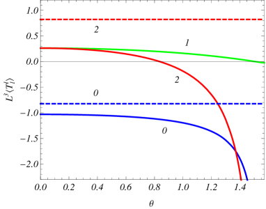
Figure 4 presents the components of the vacuum energy-momentum tensor (the numbers near the graphs correspond to the values of the index $l$) on the hemisphere cap as functions of the angle $\theta$. The dashed curves present the same quantities for the background geometry $S^{2}$. The left and right panels correspond to conformally and minimally coupled scalar fields, respectively. As before, the graphs are plotted for $ma=1/2$. For a conformally coupled field, the tube-induced part of the energy density is positive and the ${}_{2}^{2}$-stress is negative. For a minimally coupled field, the tube induced contributions are negative.

Figure 4: The vacuum energy density and stresses on the hemispherical cap as functions of $\theta$ for conformally (right panel) and minimally (right panel) coupled fields. The numbers near the curves are the values of the index $l$. The dashed lines correspond to the vacuum densities on $S^{2}$. The graphs are plotted for $ma=1/2$.

5.3 The Casimir force

The Casimir force acting per unit length of the boundary $\theta=\pi/2$ (the Casimir pressure) is determined by the normal stress evaluated at the boundary:

$$p=-\langle T_{1}^{1}\rangle_{\theta=\pi/2}.$$ (5.20)

For the side of the boundary corresponding to the tube, $\theta=\pi/2+0$, the cap-induced part in the normal stress vanishes and the Casimir pressure is directly obtained from (5.4):

$$p_{+}=\frac{\mathrm{Li}_{3}(e^{-mL})+mL\,\mathrm{Li}_{2}(e^{-mL})}{2\pi L^{3}}.$$ (5.21)

This pressure is positive and the corresponding force is directed to the direction of the cap. For a massless field

$$p_{+}=p_{0}=\frac{\zeta(3)}{2\pi L^{3}}\approx\frac{0.1913}{L^{3}}.$$ (5.22)

The pressure from the cap side is determined from (5.12) with $l=1$ evaluated at $\theta=\pi/2-0$. It is expresses in the decomposed form

$$p_{-}=p_{S^{2}}+p_{\mathrm{ind}},$$ (5.23)

where $p_{S^{2}}=-\langle T_{1}^{1}\rangle_{S^{2}}$ and the part

$$p_{\mathrm{ind}} = \frac{a^{-3}}{4\pi^{2}}\sideset{}{{}^{\prime}}{\sum}_{n=0}^{\infty}\int_{ma}^{\infty}dy\,\frac{y}{\sqrt{y^{2}-m^{2}a^{2}}}$$ (5.24)

$$\times\frac{[\sqrt{y^{2}+n^{2}}/P_{iz(y)-1/2}^{-n\prime}+1/P_{iz(y)-1/2}^{-n}]^{2}}{\Gamma(n+iz(y)+1/2)\Gamma(n-iz(y)+1/2)},$$

is induced by the geometry of the tube. In deriving this formula we have used the expressions (2.17) and the relation (2.25). The numerical calculations show that the Casimir pressures from different sides of the boundary are equal to each other, i.e., $p_{+}=p_{-}$, and, hence, the net Casimir force on the boundary vanishes. This is related to the smooth transition between two subspaces and to the fact that the extrinsic curvature tensor of the separating boundary vanishes for both sides.

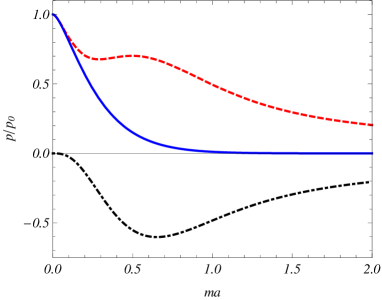
In figure 5, for a conformally coupled scalar field, we have plotted the ratio of the Casimir pressure $p=p_{-}=p_{+}$ to $p_{0}$, defined by (5.22), as a function of $ma$. We have also presented the parts corresponding to the separate terms in the rhs of (5.23). The dot-dashed curve corresponds to the ratio $p_{S^{2}}/p_{0}$ (the part corresponding to the pressure in the geometry of $S^{2}$) and the dashed curve corresponds to the ratio for the tube-induced part, $p_{\mathrm{ind}}/p_{0}$. Note that for large values of the mass, the decay of the separate terms in the rhs of (5.23), as functions of $ma$, is as power-law, whereas the total pressure decays exponentially. The latter follows from the equality $p_{+}=p_{-}$ and from the exponential decay of $p_{+}$ for large masses.

Figure 5: The ratio of the Casimir pressure on the separating boundary to the corresponding pressure for a massless field, as a function of $ma$. The dot-dashed curve corresponds to the ratio $p_{S^{2}}/p_{0}$ and the dashed curve is for $p_{\mathrm{ind}}/p_{0}$.

6 Conclusion

In the present paper we have considered the properties of the quantum vacuum for a $(2+1)$-dimensional scalar field in a background geometry of a cylindrical tube with a hemispherical cap. In this geometry one has two spatial regions with different geometrical characteristics separated by a circular boundary. Our main interest was to investigate the changes in the local characteristics of the vacuum induced by the geometry of the attached region. In free field theories with only interaction of the background gravitational field, all the information about the properties of the vacuum state is encoded in two-point functions. As such we have evaluated the positive frequency Wightman function by using the direct summation method over a complete set of modes. In the problem under consideration the metric tensor and its first derivatives are continuous at the separating boundary and, as a consequence, the mode functions and their normal derivatives are continuous as well. For continuous energy spectrum these functions in separate regions are given by (2.20) and (2.21) with the relations (2.14) and (2.15) between the constants. In addition, for negative values of the curvature coupling parameter $\xi$ there are bound states. In both the cylindrical and hemispherical subspaces, we explicitly separated the contributions in the Wightman function induced by the geometry of the attached region. These contributions are given by the second term in the rhs of (3.5) for points on the tube and by the second term in the rhs of (3.13) for the hemispherical cap. With this separation, the renormalization of the VEVs in the coincidence limit is reduced to that for an infinite cylinder and for two-dimensional sphere $S^{2}$.

As an important local characteristic of the vacuum state, in section 4 we have studied the VEV of the field squared. On the tube this VEV is given by (4.1), where the second term in the rhs is the contribution induced by the hemispherical cap. Unlike to the case of a semi-infinite tube with Dirichlet or Neumann boundary conditions on its edge, where the mean field squared diverges on the boundary, in the problem at hand the VEV of the field squared is finite everywhere. At large distances from the separating boundary and for a massive field, the contribution in the mean field squared induced by the cap is exponentially small (see (4.4)) and the total VEV is dominated by the part corresponding to an infinite tube. The latter is positive everywhere. For points on the hemispherical cap the VEV of the field squared is presented in the decomposed form (4.6). The tube-induced part, given by the second term in the rhs, is finite everywhere including the points on the boundary. Though the Wightman function is continuous at the separating circle, the renormalized VEV of the field squared has discontinuity. This is related to the fact that in the renormalization procedure for tubular and hemispherical geometries different terms are subtracted. On the hemisphere, in addition to the Minkowskian term, we have also subtracted a finite renormalization term (see appendix A). In the minimal subtraction scheme, where the only Minkowskian part is subtracted for both regions, the mean field squared is continuous at the boundary. In the numerical examples, we have considered the most important special cases of minimally and conformally coupled scalar fields. For both these cases the cap-induced contributions in the VEV of the field squared on the tube are positive, whereas the tube-induced contributions on the cap are negative.

Another important characteristic of the ground state is the VEV of the energy-momentum tensor. This VEV is diagonal and obeys the trace relation (5.8). On the tube the vacuum energy-momentum tensor is given by the expression (5.2) with the infinite tube part from (5.4). The cap-induced part in the vacuum stress normal to the boundary vanishes. The energy density and the parallel stress diverge on the boundary. The leading terms in the corresponding asymptotic expansion over the distance from the boundary are given by (5.9). In the geometry of a semi-infinite tube with Dirichlet or Neumann boundary conditions on the edge, the divergences are stronger, the VEVs diverge as the inverse cube of the distance from the edge. At large distances from the boundary and for a massive field, the cup-induced contribution in the energy-momentum tensor is exponentially small, whereas for a massless field it decays as the inverse square of the distance. For numerical examples displayed in figure 3, the cup-induced contribution to the energy density is positive for both conformally and minimally coupled field. The corresponding parallel stress is negative for a conformally coupled field and positive for a minimally coupled field.

The vacuum energy-momentum tensor on the cap is decomposed as (5.12), where the components for the part corresponding to $S^{2}$ are given by (B.12) and (B.14). We have explicitly checked that the VEV obeys the covariant conservation equation, which for the geometry of the cup is reduced to the relation (5.15). The energy density and the parallel stress diverge on the separating circle and the expression for the corresponding leading terms in the asymptotic expansion over $\theta-\pi/2$ coincide with those on the tube. On the cap and on the tube these components have opposite signs. The normal stress is finite everywhere. It determines the Casimir force acting on the boundary. From the sides of the tube and of the cap the vacuum pressures on the boundary are given by the expressions (5.21) and (5.23) respectively. We have checked numerically that these pressures coincide and, hence, the net Casimir force on the boundary is zero.

The results obtained above may be applied to carbon nanotubes with half fullerene caps, described in the long-wavelength approximation by an effective field theory. As has been mentioned in Introduction, the latter, in addition to Dirac fermions, involves scalar and gauge fields as well.

Appendix A Proof of the identity with Legendre functions

In this appendix we prove the identity which is used in section 3 for the decomposition of the Wightman function on the hemispherical cap. Let us define the function

$$R_{\lambda-1/2}^{\mu}(u)=Q_{-\lambda-1/2}^{\mu}(u)\cos[\pi(\mu-\lambda)]+Q_{\lambda-1/2}^{\mu}(u)\cos[\pi(\mu+\lambda)],$$ (A.1)

where $u=\cos\theta$ and $Q_{\lambda-1/2}^{\mu}(u)$ is the associated Legendre function of the second kind. By using the relation [25]

$$Q_{-\lambda-1/2}^{\mu}(u)\cos[\pi(\mu-\lambda)]=Q_{\lambda-1/2}^{\mu}(u)\cos[\pi(\mu+\lambda)]+\pi\cos(\mu\pi)\sin(\lambda\pi)P_{\lambda-1/2}^{\mu}(u),$$ (A.2)

the function (A.1) can also be expressed as a linear combination of the functions $P_{\lambda-1/2}^{\mu}(u)$ and $Q_{\lambda-1/2}^{\mu}(u)$. Next, we introduce the notations

$$\bar{P}_{\lambda-1/2}^{\pm,\mu}(u) = \partial_{\theta}P_{\lambda-1/2}^{\mu}(u)\mp ipP_{\lambda-1/2}^{\mu}(u),$$

$$\bar{R}_{\lambda-1/2}^{\pm,\mu}(u) = \partial_{\theta}R_{\lambda-1/2}^{\mu}(u)\mp ipR_{\lambda-1/2}^{\mu}(u).$$ (A.3)

We want to prove the identity

$$\frac{\cos[\pi(\mu+\lambda)]}{\bar{P}_{\lambda-1/2}^{+,\mu}(u)\bar{P}_{\lambda-1/2}^{-,\mu}(u)}=i\frac{\sin\theta}{4p}\frac{\Gamma(\lambda-\mu+1/2)}{\Gamma(\lambda+\mu+1/2)}\sum_{j=+,-}j\frac{\bar{R}_{\lambda-1/2}^{j,\mu}(u)}{\bar{P}_{\lambda-1/2}^{j,\mu}(u)}.$$ (A.4)

For the sum in the rhs of (A.4) one has

$$\sum_{j=+,-}j\frac{\bar{R}_{\lambda-1/2}^{j,\mu}(u)}{\bar{P}_{\lambda-1/2}^{j,\mu}(u)}=-2ip\frac{R_{\lambda-1/2}^{\mu}(u)\partial_{\theta}P_{\lambda-1/2}^{\mu}(u)-P_{\lambda-1/2}^{\mu}(u)\partial_{\theta}R_{\lambda-1/2}^{\mu}(u)}{\bar{P}_{\lambda-1/2}^{+,\mu}(u)\bar{P}_{\lambda-1/2}^{-,\mu}(u)}.$$ (A.5)

By using the Wronskian for the associated Legendre functions we can see that

$$Q_{\lambda-1/2}^{\mu}(u)\partial_{\theta}P_{\lambda-1/2}^{\mu}(u)-P_{\lambda-1/2}^{\mu}(u)\partial_{\theta}Q_{\lambda-1/2}^{\mu}(u)=\frac{\Gamma(\lambda+\mu+1/2)}{\sin\theta\Gamma(\lambda-\mu+1/2)}.$$ (A.6)

Combining this with the relation (A.2), for the numerator in (A.5) we get

$$R_{\lambda-1/2}^{\mu}(u)\partial_{\theta}P_{\lambda-1/2}^{\mu}(u)-P_{\lambda-1/2}^{\mu}(u)\partial_{\theta}R_{\lambda-1/2}^{\mu}(u)=\frac{2\Gamma(\lambda+\mu+1/2)}{\sin\theta\Gamma(\lambda-\mu+1/2)}\cos[\pi(\mu+\lambda)].$$ (A.7)

The identity (A.4) directly follows from (A.5) and (A.7).

For $\mu=-n$ from (A.4) one has

$$\frac{1}{\bar{P}_{\lambda-1/2}^{+,-n}(u)\bar{P}_{\lambda-1/2}^{-,-n}(u)}=i\frac{\sin\theta}{4p}\frac{\Gamma(\lambda+n+1/2)}{\Gamma(\lambda-n+1/2)}\sum_{j=+,-}j\frac{\bar{S}_{\lambda-1/2}^{j,-n}(u)}{\bar{P}_{\lambda-1/2}^{j,-n}(u)},$$ (A.8)

where we have defined a new function

$$S_{\lambda-1/2}^{-n}(u)=Q_{\lambda-1/2}^{-n}(u)+Q_{-\lambda-1/2}^{-n}(u),$$ (A.9)

and, similar to (A.3),

$$\bar{S}_{\lambda-1/2}^{\pm,\mu}(u)=\partial_{\theta}S_{\lambda-1/2}^{\mu}(u)\mp ipS_{\lambda-1/2}^{\mu}(u).$$ (A.10)

Note that, by using the relation (A.2), the function (A.9) can also be written in the form

$$S_{\lambda-1/2}^{-n}(x)=2Q_{\lambda-1/2}^{-n}(u)+\pi\tan(\lambda\pi)P_{\lambda-1/2}^{-n}(u).$$ (A.11)

By making use of the trigonometric expansions of the functions $P_{\lambda-1/2}^{-n}(u)$ and $Q_{\lambda-1/2}^{-n}(u)$ [25], the following expansion is obtained for the function (A.9):

$$S_{\lambda-1/2}^{-n}(u) = \frac{2^{1-n}}{\sin^{n}\theta}\frac{\sqrt{\pi}\Gamma(\lambda-n+1/2)}{\Gamma(\lambda+1)\cos(\lambda\pi)}\sum_{l=0}^{\infty}\frac{(1/2-n)_{l}(\lambda-n+1/2)_{l}}{l!(\lambda+1)_{l}}$$ (A.12)

$$\times\cos\left[\left(2l-n+1/2\right)\theta-\lambda\left(\pi-\theta\right)\right],$$

where $(b)_{l}$ is Pochhammer’s symbol, $u=\cos\theta$ and $0<\theta<\pi$. From here it follows that in the complex plane $\lambda$ the function $S_{\lambda-1/2}^{-n}(u)$ decays exponentially in the limit $|\mathrm{Im}\,\lambda|\rightarrow\infty$. Note that in the same limit the function $P_{\lambda-1/2}^{-n}(u)$ increases exponentially.

Appendix B Casimir densities on $S^{2}$

In this appendix we consider the vacuum densities for a scalar field on $S^{2}$ (for the Casimir energy in spherical universes see [31] and references therein). The corresponding vacuum energy and stresses for a conformally coupled field have been investigated in [16]. The mode functions on $S^{2}$, regular for $0\leqslant\theta<\pi$, have the form (2.20). From the regularity of these functions at $\theta=\pi$ it follows that $\lambda-1/2=l$ with $l=|n|,|n|+1,\ldots$. Hence, the modes are specified by the set $\sigma=(l,n)$ and have the form

$$\varphi_{\sigma}(x)=C_{0\mathrm{s}}P_{l}^{-|n|}(\cos\theta)e^{in\phi-i\omega_{l}t},\;0\leqslant\theta\leqslant\pi,$$ (B.1)

where $|n|\leqslant l$, $l=0,1,2,\ldots$, and the energy $\omega_{l}$ is given by the expression (3.16). From the normalization condition one gets

$$|C_{0\mathrm{s}}|^{2}=\frac{l+1/2}{4\pi a^{2}\omega_{l}}\frac{\Gamma(l+|n|+1)}{\Gamma(l-|n|+1)}.$$ (B.2)

Substituting the functions (B.1) into the mode-sum, after the summation over $n$ by using (3.14), we obtain the expression (3.15) for the Wightman function on $S^{2}$. Note that the latter obeys the relation

$$\partial_{a}[a^{3}\lim_{t^{\prime}\rightarrow t}\partial_{t^{\prime}}\partial_{t}W_{S^{2}}(x,x^{\prime})]=m^{2}a^{2}\lim_{t^{\prime}\rightarrow t}W_{S^{2}}(x,x^{\prime}).$$ (B.3)

As will be seen below, this leads to the relation between the vacuum energy and the VEV of the field squared.

For the VEV of the field squared we find

$$\langle\varphi^{2}\rangle_{S^{2}}=\frac{a^{-2}}{4\pi}\sum_{l=0}^{\infty}\frac{l+1/2}{\omega_{l}}.$$ (B.4)

Of course this expression is divergent and needs to be renormalized. Here we note that in $(2+1)$-dimensions the divergence of the Wightman function in the coincidence limit is the same as in Minkowski spacetime. Hence, the subtraction of the Minkowskian part from (B.4) gives a finite result. The unrenormalized VEV of the field squared in the Minkowski spacetime is given by the expression

$$\langle\varphi^{2}\rangle_{M}=\frac{1}{4\pi}\int_{0}^{\infty}dx\,\frac{x}{\sqrt{x^{2}+m^{2}}}.$$ (B.5)

However, in the renormalization procedure, we need also to subtract the next to the leading term in DeWitt-Schwinger expansion.

First we assume that $m^{2}a^{2}+2\xi\geqslant 1/4$. In this case, applying the Abel-Plana summation formula in the form [16, 26]

$$\sum_{l=0}^{\infty}f(l+1/2)=\int_{0}^{\infty}dx\,f(x)-i\int_{0}^{\infty}dx\,\frac{f(ix)-f(-ix)}{e^{2\pi x}+1},$$ (B.6)

and subtracting the first two terms of DeWitt-Schwinger expansion, from (B.4) for the renormalized VEV of the field squared we get

$$\langle\varphi^{2}\rangle_{S^{2}}=\frac{m}{4\pi}\left[1+\frac{\xi-1/6}{m^{2}a^{2}}-b_{m}+2b_{m}\int_{0}^{1}dx\,\frac{x(1-x^{2})^{-1/2}}{e^{2\pi\omega_{m}x}+1}\right],$$ (B.7)

with the notation $b_{m}=\omega_{m}/(ma)$. The second term in the square brackets of (B.7) comes from the next to the leading term in DeWitt-Schwinger expansion. For large masses, $ma\gg 1$, one has

$$\langle\varphi^{2}\rangle_{S^{2}}\approx\frac{m^{-3}}{2^{9}\pi a^{4}}\left[\frac{7}{15}+\left(8\xi-1\right)^{2}\right],$$ (B.8)

and the VEV decays as $m^{-3}$.

The VEV of the energy-momentum tensor is evaluated by using the formula (5.1) with the Wightman function from (3.15). For the unrenormalized energy density we get

$$\langle T_{0}^{0}\rangle_{S^{2}}=\frac{a^{-3}}{4\pi}\sum_{l=0}^{\infty}(l+1/2)\sqrt{(l+1/2)^{2}+\omega_{m}^{2}},$$ (B.9)

and for the stresses one has the relation

$$\langle T_{1}^{1}\rangle_{S^{2}}=\langle T_{2}^{2}\rangle_{S^{2}}=-\frac{1}{2}\langle T_{0}^{0}\rangle_{S^{2}}+\frac{1}{2}m^{2}\langle\varphi^{2}\rangle_{S^{2}}.$$ (B.10)

Note that the VEVs obey the trace relation (5.8). For the renormalization we need to subtract from the VEVs the corresponding DeWitt-Schwinger expansion truncated at the adiabatic order 3.

An alternative way is to use the relation $\partial_{a}\left(a^{3}\langle T_{0}^{0}\rangle_{S^{2}}\right)=m^{2}a^{2}\langle\varphi^{2}\rangle_{S^{2}}$, which directly follows from (B.3). From this relation for the renormalized VEV of the energy density we get

$$\langle T_{0}^{0}\rangle_{S^{2}}=\frac{m^{2}}{a^{3}}\int da\,a^{2}\langle\varphi^{2}\rangle_{S^{2}}.$$ (B.11)

By taking into account the expression (B.7), one finds

$$\langle T_{0}^{0}\rangle_{S^{2}}=\frac{m^{3}}{4\pi}\,\left(\frac{1}{3}+\frac{\xi-1/6}{m^{2}a^{2}}-\frac{b_{m}^{3}}{3}+2b_{m}^{3}\int_{0}^{1}dx\,\frac{x\sqrt{1-x^{2}}}{e^{2\pi\omega_{m}x}+1}\right).$$ (B.12)

For large values of the mass we have the leading term

$$\langle T_{0}^{0}\rangle_{S^{2}}\approx-\frac{a^{-4}}{8\pi m}\,\left[\frac{7}{960}+\left(\xi-\frac{1}{8}\right)\left(\xi-\frac{5}{24}\right)\right],$$ (B.13)

and the renormalized VEV vanishes in the limit $m\rightarrow\infty$. Note that the relation (B.11) determines the renormalized energy density up to the term $C(m)/a^{3}$, where the function $C(m)$ is dimensionless. By taking into account that the only dimensionful quantity to form this function is the mass $m$, we conclude that $C(m)$ does not depend on $m$. Now, imposing the renormalization condition (for a discussion of this condition see [16]) $\langle T_{0}^{0}\rangle_{S^{2}}\rightarrow 0$ in the limit $m\rightarrow\infty$, we see that $C(m)=0$. The stresses are found from the relation (B.10):

$$\langle T_{1}^{1}\rangle_{S^{2}} = \frac{m^{3}}{8\pi}\left\{2b_{m}^{3}\int_{0}^{1}dx\,\frac{x^{3}/\sqrt{1-x^{2}}}{e^{2\pi\omega_{m}x}+1}-\left(b_{m}-\,1\right)\right.$$ (B.14)

$$\times\left.\left[\frac{2}{3}+b_{m}\left(b_{m}+1\right)\left(2\int_{0}^{1}dx\,\frac{x/\sqrt{1-x^{2}}}{e^{2\pi\omega_{m}x}+1}-\frac{1}{3}\right)\right]\right\}.$$

In the limit of large masses, to the leading order one has $\langle T_{1}^{1}\rangle_{S^{2}}\approx-\langle T_{0}^{0}\rangle_{S^{2}}$ with the asymptotic expression for the energy density given by (B.13). For a conformally coupled scalar field $b_{m}=1$ and (B.14) reduces to the expression given in [16]. In the same limit, (B.12) reduces to the corresponding result in [16] up to a finite renormalization term $-m/(96a^{2})$. Note that without this term the renormalized energy density does not vanish in the limit $m\rightarrow\infty$. For both minimally and conformally coupled fields the energy density (B.12) is negative and the stress (B.14) is positive. For a massless conformally coupled field the VEV $\langle T_{i}^{k}\rangle_{S^{2}}$ vanishes.

The combination of (B.10) and (B.11), leads to the relation

$$\langle T_{1}^{1}\rangle_{S^{2}}=\partial_{V}E_{S^{2}},$$ (B.15)

where $V=4\pi a^{2}$ is the volume of the space and $E_{S^{2}}=V\langle T_{0}^{0}\rangle_{S^{2}}$ is the total vacuum energy. This is the standard thermodynamical relation between the energy and the pressure.

Now let us consider the case $m^{2}a^{2}+2\xi\leqslant 1/4$. In this case the function $f(x)$, corresponding to (B.4), has a branch point in the right half-plane and the formula (B.6) needs a generalization. As the starting point we us the Abel-Plana formula in its initial form (see, for instance, [16, 26]) for series $\sum_{l=0}^{\infty}f(l)$. Taking $f(x)=g(x)/\sqrt{x^{2}-x_{0}^{2}}$, by the transformation of the integration contour in the rhs, the following formula can be obtained

$$\sum_{l=0}^{\infty}\frac{g(l+1/2)}{\sqrt{(l+1/2)^{2}-x_{0}^{2}}} = \int_{x_{0}}^{\infty}dx\,\frac{g(x)}{\sqrt{x^{2}-x_{0}^{2}}}+\int_{0}^{x_{0}}dx\,\frac{\tan(\pi x)}{\sqrt{x_{0}^{2}-x^{2}}}g(x)$$ (B.16)

$$-\int_{0}^{\infty}dx\,\frac{g(ix)+g(-ix)}{\sqrt{x^{2}+x_{0}^{2}}(e^{2\pi x}+1)},$$

for $x_{0}<1/2$ and for a function $g(x)$ analytic in the right half-plane. Note that for the series in (B.4) one has $g(x)=x$ and the last integral in (B.16) vanishes.

Further evaluation of the renormalized VEVs is similar to that we have described above for the case $m^{2}a^{2}+2\xi\geqslant 1/4$. Applying to the series in (B.4) the formula (B.16) with $x_{0}^{2}=-\omega_{m}^{2}\geqslant 0$, after the renormalization, for the VEV of the field squared one gets

$$\langle\varphi^{2}\rangle_{S^{2}}=\frac{m}{4\pi}\left[1+\frac{\xi-1/6}{m^{2}a^{2}}+\frac{|\omega_{m}|}{ma}\int_{0}^{1}dy\,\tan(\pi|\omega_{m}|\sqrt{1-y^{2}})\right].$$ (B.17)

The VEV of the energy density is found from (B.11). This leads to the expression

$$\langle T_{0}^{0}\rangle_{S^{2}}=\frac{m^{3}}{4\pi}\left[\frac{1}{3}+\,\frac{\xi-1/6}{m^{2}a^{2}}-\frac{|\omega_{m}|^{3}}{m^{3}a^{3}}\int_{0}^{1}dy\,y^{2}\tan(\pi|\omega_{m}|\sqrt{1-y^{2}})\right].$$ (B.18)

The integration constant is determined from the continuity of the energy density at $\omega_{m}=0$. The stresses are obtained by making use of the relation (B.10).

References

- [1] S. Deser, R. Jackiw, and S. Templeton, Ann. Phys. 140, 372 (1982).
- [2] A.J. Niemi and G.W. Semenoff, Phys. Rev. Lett. 51, 2077 (1983); R. Jackiw, Phys. Rev. D 29, 2375 (1984); A.N. Redlich, Phys. Rev. D 29, 2366 (1984); M.B. Paranjape, Phys. Rev. Lett. 55, 2390 (1985); D. Boyanovsky and R. Blankenbecler, Phys. Rev. D 31, 3234 (1985); R. Blankenbecler and D. Boyanovsky, Phys. Rev. D 34, 612 (1986).
- [3] T. Jaroszewicz, Phys. Rev. D 34, 3128 (1986); E.G. Flekkøy and J.M. Leinaas, Int. J. Mod. Phys. A 6, 5327 (1991); H. Li, D.A. Coker, and A.S. Goldhaber, Phys. Rev. D 47, 694 (1993).
- [4] F. Wilczek, Fractional Statistics and Anyon Superconductivity (World Scientific, Singapore, 1990).
- [5] V.P. Gusynin, V.A. Miransky and L.A. Shovkovy, Phys. Rev. D 52, 4718 (1995); R.R. Parwani, Phys. Lett. B 358, 101 (1995).
- [6] Yu.A. Sitenko, Phys. At. Nucl. 60, 2102 (1997); Yu.A. Sitenko, Phys. Rev. D 60, 125017 (1999).
- [7] G.V. Dunne, Topological Aspects of Low Dimensional Systems (Springer, Berlin, 1999).
- [8] D.J. Gross, R.D. Pisarski, and L.G. Yaffe, Rev. Mod. Phys. 53, 43 (1981).
- [9] N. Dorey and N.E. Mavromatos, Nucl. Phys. B 386, 614 (1992); M. Franz, Z. Tesanovic, and O. Vafek, Phys. Rev. B 66, 054535 (2002); I.F. Herbut, Phys. Rev. B 66, 094504 (2002); I.O. Thomas and S. Hands, Phys. Rev. B 75, 134516 (2007).
- [10] V.P. Gusynin, S.G. Sharapov, and J.P. Carbotte, Int. J. Mod. Phys. B 21, 4611 (2007); A.H. Castro Neto, F. Guinea, N.M.R. Peres, K.S. Novoselov, and A.K. Geim, Rev. Mod. Phys. 81, 109 (2009).
- [11] M.Z. Hasan and C.L. Cane, Rev. Mod. Phys. 82, 3045 (2010); J. H. Bardarson and J. E. Moore, Rep. Prog. Phys. 76, 056501 (2013).
- [12] R. Jackiw and S.-Y. Pi, Phys. Rev. Lett. 98, 266402 (2007); O. Oliveira, C.E. Cordeiro, A. Delfino, W. de Paula, and T. Frederico, Phys. Rev. B 83, 155419 (2011).
- [13] S. Bellucci and A.A. Saharian, Phys. Rev. D 79, 085019 (2009); S. Bellucci, A.A. Saharian, and V.M. Bardeghyan, Phys. Rev. D 82, 065011 (2010).
- [14] S. Bellucci, E. R. Bezerra de Mello, and A. A. Saharian, Phys. Rev. D 89, 085002 (2014).
- [15] M.S. Dresselhaus, G. Dresselhaus, and R. Saito, Phys. Rev. B 45, 6234 (1992); G. Brinkmann, P.W. Fowler, D.E. Manolopoulos, and A.H.R. Palser, Chem. Phys. Lett. 315, 335 (1999); T. Y. Astakhova, G.A. Vinogradov, and E. Osawa, Full. Sci. Tech. 7, 769 (1999); S. Reich, L. Li, and J. Robertson, Phys. Rev. B 72, 165423 (2005); M. Robinson, I. Suarez-Martinez, and N. A. Marks, Phys. Rev. B 87, 155430 (2013).
- [16] M. Bordag, G.L. Klimchitskaya, U. Mohideen, and V.M. Mostepanenko, Advances in the Casimir Effect (Oxford University Press, Oxford, 2009); M. Bordag, U. Mohideen, and V.M. Mostepanenko, Phys. Rep. 353, 1 (2001).
- [17] G. Plunien, B. Müller, and W. Greiner, Phys. Rep. 134, 87 (1986); E. Elizalde, S.D. Odintsov, A. Romeo, A.A. Bytsenko, and S. Zerbini, Zeta Regularization Techniques with Applications (World Scientific, Singapore, 1994); V.M. Mostepanenko and N.N. Trunov, The Casimir Effect and its Applications (Clarendon, Oxford, 1997); K.A. Milton, The Casimir Effect: Physical Manifestation of Zero-Point Energy (World Scientific, Singapore, 2002); Casimir Physics, edited by D. Dalvit, P. Milonni, D. Roberts, and F. da Rosa, Lecture Notes in Physics Vol. 834 (Springer-Verlag, Berlin, 2011).
- [18] S. Bellucci and A. A. Saharian, Phys. Rev. D 79, 085019 (2009); E. Elizalde, S.D. Odintsov, and A.A. Saharian, Phys. Rev. D 83, 105023 (2011).
- [19] E.R. Bezerra de Mello, V.B. Bezerra, A.A. Saharian, and A.S. Tarloyan, Phys. Rev. D 74, 025017 (2006).
- [20] E.R. Bezerra de Mello and A.A. Saharian, J. High Energy Phys. 10 (2006) 049; E.R. Bezerra de Mello and A.A. Saharian, Phys. Rev. D 75, 065019 (2007); E.R. Bezerra de Mello and A.A. Saharian, Class. Quantum Grav. 29, 135007 (2012).
- [21] W.A. Hiscock, Phys. Rev. D 31, 3288 (1985); J.R. Gott, Astrophys. J. 288, 422 (1985).
- [22] B. Allen and A.C. Ottewill, Phys. Rev. D 42, 2669 (1990).
- [23] K. Milton and A.A. Saharian, Phys. Rev. D 85, 064005 (2012); S. Bellucci, A.A. Saharian, and A.H. Yeranyan, Phys. Rev. D 89, 105006 (2014); S. Bellucci, A.A. Saharian, and N.A. Saharyan, arXiv:1407.0879.
- [24] A.A. Saharian and A.L. Mkhitaryan, J. High Energy Phys. 08 (2007) 063; A.A. Saharian and A.L. Mkhitaryan, J. Phys. A: Math. Theor. 41, 164062 (2008).
- [25] A. Erdélyi et al., Higher Transcendental Functions (McGraw Hill, New York, 1953), Vol. 1.
- [26] A.A. Saharian, The Generalized Abel-Plana Formula with Applications to Bessel Functions and Casimir Effect (Yerevan State University Publishing House, Yerevan, 2008); Report No. ICTP/2007/082; arXiv:0708.1187.
- [27] A. Flachi and G. Fucci, J. Math. Phys. 52, 023503 (2011); G. Fucci and K. Kirsten, Commun. Math. Phys. 314, 483 (2012).
- [28] N.D. Birrell and P.C.W. Davies, Quantum Fields in Curved Space (Cambridge University Press, Cambridge, England, 1982).
- [29] A.A. Saharian, Phys. Rev. D 69, 085005 (2004).
- [30] N.R. Khusnutdinov, J. Math. Phys. 44, 2320 (2003); R.C. Thorne, Philos. Trans. R. Soc. London A 249, 597 (1957).
- [31] L.H. Ford, Phys. Rev. D 11, 3370 (1975); J.S. Dowker and R. Critchley, Phys. Rev. D 15, 1484 (1977); P. Candelas and S. Weinberg, Nucl. Phys. B 237, 397 (1984); R. Kantowski and K.A. Milton, Phys. Rev. D 35, 549 (1987); E. Elizalde, J. Math. Phys. 35, 3308 (1994); A. Zhuk and H. Kleinert, Theor. Math. Phys. 109, 1483 (1996); A.A. Bytsenko, G. Cognola, L. Vanzo, and S. Zerbini, Phys. Rep. 266, 1 (1996); I. Brevik, K.A. Milton, and S.D. Odintsov, Ann. Phys. (NY) 302, 120 (2002); M. Öscan, Class. Quantum Grav. 23, 5531 (2006); C.A.R. Herdeiro, R.H. Ribeiro, and M. Sampaio, Class. Quantum Grav. 25, 165010 (2008); V.B. Bezerra, G.L. Klimchitskaya, V.M. Mostepanenko, and C. Romero, Phys. Rev. D 83, 104042 (2011); V.B. Bezerra, V.M. Mostepanenko, H.F. Mota, and C. Romero, Phys. Rev. D 84, 104025 (2011).