CLASH-VLT: The stellar mass function and stellar mass density profile of the z=0.44 cluster of galaxies MACS J1206.2-0847

Abstract

Context. The study of the galaxy stellar mass function (SMF) in relation to the galaxy environment and the stellar mass density profile, $\mathrm{\rho_{\star}(r)}$,is a powerful tool to constrain models of galaxy evolution.

Aims. We determine the SMF of the z=0.44 cluster of galaxies MACS J1206.2-0847 separately for passive and star-forming (SF) galaxies, in different regions of the cluster, from the center out to approximately 2 virial radii. We also determine $\mathrm{\rho_{\star}(r)}$ to compare it to the number density and total mass density profiles.

Methods. We use the dataset from the CLASH-VLT survey. Stellar masses are obtained by spectral energy distribution fitting with the MAGPHYS technique on 5-band photometric data obtained at the Subaru telescope. We identify 1363 cluster members down to a stellar mass of $10^{9.5}\rm{M}_{\odot}$, selected on the basis of their spectroscopic ($\sim 1/3$ of the total) and photometric redshifts. We correct our sample for incompleteness and contamination by non members. Cluster member environments are defined using either the clustercentric radius or the local galaxy number density.

Results. The whole cluster SMF is well fitted by a double Schechter function, which is the sum of the two Schechter functions that provide good fits to the SMFs of, separately, the passive and SF cluster populations. The SMF of SF galaxies is significantly steeper than the SMF of passive galaxies at the faint end. The SMF of the SF cluster galaxies does not depend on the environment. The SMF of the passive cluster galaxies has a significantly smaller slope (in absolute value) in the innermost ($\leq 0.50$ Mpc, i.e., $\sim 0.25$ virial radii), and in the highest density cluster region than in more external, lower density regions. The number ratio of giant/subgiant galaxies is maximum in this innermost region and minimum in the adjacent region, but then gently increases again toward the cluster outskirts. This is also reflected in a decreasing radial trend of the average stellar mass per cluster galaxy. On the other hand, the stellar mass fraction, i.e., the ratio of stellar to total cluster mass, does not show any significant radial trend.

Conclusions. Our results appear consistent with a scenario in which SF galaxies evolve into passive galaxies due to density-dependent environmental processes, and eventually get destroyed very near the cluster center to become part of a diffuse intracluster medium. Dynamical friction, on the other hand, does not seem to play an important role. Future investigations of other clusters of the CLASH-VLT sample will allow us to confirm our interpretation.

1 Introduction

Many galaxy properties, such as colors, luminosities, morphologies, star formation rates, and stellar masses, follow a bimodal distribution (e.g., Baldry et al. 2004; Kauffmann et al. 2003). Galaxies can therefore be classified in two broad classes, red, bulge-dominated, high-mass, passively-evolving galaxies, and blue, disk-dominated, low-mass, star-forming galaxies. The relative number fraction of these two populations changes with redshift (z) and with the local galaxy number density, blue galaxies dominating at higher z and in lower density environments (see Silk & Mamon 2012 for a recent review on galaxy formation and evolution). This suggests that the redshift evolution of these two populations is somehow shaped by physical processes related to the environment in which they reside, such as major and minor mergers, tidal interactions among galaxies or between a galaxy and a cluster gravitational field, and ram-pressure stripping (see, e.g., Biviano 2008 and references therein). All these processes use or remove gas from galaxies, leading to a drop in star-formation due to lack of fuel and to an aging of the stellar population, and consequent reddening of the galaxy light with time. Some of these processes also lead to morphological transformations. These quenching mechanisms have been implemented in both N-body simulations and semi-analytical models with the aim of reproducing the phenomenology of galaxy evolution, and in particular the changing fraction of red and blue galaxies with time. However, there are still many discrepancies between observations and theoretical predictions, such as, e.g., the evolution of galaxy colors, luminosities, and stellar masses (e.g., Cucciati et al. 2012; De Lucia et al. 2012; Silk & Mamon 2012 and references therein).

The distributions of galaxy luminosities and stellar masses ($\rm{M}_{\star}$ hereafter), namely, the galaxy luminosity and stellar mass functions (SMF hereafter), are key observables for testing galaxy evolutionary models (e.g., Macciò et al. 2010; Menci et al. 2012). The SMF allows for a more direct test of theoretical models than the luminosity function, since luminosities are more difficult to predict than $\rm{M}_{\star}$ because of effects such as the age and metallicity of the stellar population, the dust content of the interstellar medium, etc. On the other hand, unlike luminosities, $\rm{M}_{\star}$ are not direct observables, and can be determined only via multicolor and/or near infrared photometry. This explains why most studies of the galaxy SMF have been conducted only quite recently.

Most determinations of the galaxy SMF (or of the near-infrared luminosity function, which is considered a proxy for the SMF) have been based on samples of field galaxies. The field galaxy SMF appears to have a flat slope down to $10^{9}\rm{M}_{\odot}$, up to $\mathrm{z}\sim 1$ (Fontana et al., 2006) and beyond (Stefanon & Marchesini, 2013; Sobral et al. 2014), although some authors provide evidence that the SMF steepens with z (Mortlock et al. 2011; Bielby et al. 2012; Huang et al. 2013). Ilbert et al. (2010) find that this steepening occurs at masses lower than a certain limit, which varies with z, and results from the combination of two single Schechter (1976) functions that characterize, separately, the red and blue SMF (Bolzonella et al. 2010; Ilbert et al. 2010; Pozzetti et al. 2010).

To highlight possible environmental effects on the galaxy SMF one should compare the field galaxy SMF to that of cluster galaxies. Balogh et al. (2001) have found the SMF of non emission line galaxies to be steeper in clusters than in the field. On the other hand, Vulcani et al. (2012, 2013) have found the field and cluster SMF not to be different, at least down to $\rm{M}_{\star}\sim 10^{10.2}\rm{M}_{\odot}$, not even when considering different galaxy populations separately. Their analysis is based on optical magnitudes and colors, while Balogh et al. (2001) use J-band magnitudes. Other studies of the near infrared luminosity functions of cluster and field galaxies found them to be statistically indistinguishable (Lin et al. 2004a; Strazzullo et al. 2006; and De Propris & Christlein 2009). Giodini et al. (2012) find no major difference between the SMF of field and group SF galaxies, at any redshift, and down to $\sim 10^{8.5}\rm{M}_{\odot}$, except at the high-mass end, however, they do find significant differences in the SMF of passive galaxies in the field and low-mass groups, on one side, and in high-mass groups, on the other. Within clusters, there is no difference in the global SMFs evaluated within and outside the virial region (Vulcani et al. 2013), but Calvi et al. (2013) find the SMFs of different galaxy types change within different cluster environments.

Different results might be caused by the different $\rm{M}_{\star}$ completeness limits reached by the different studies. Merluzzi et al. (2010) suggest that at low z the environmental dependence of the SMF becomes evident only for masses below $\sim 10^{9}\,\rm{M}_{\odot}$. At $\mathrm{z}\sim 1$ an environmental dependence of the SMF is already seen at the $10^{10}\,\rm{M}_{\odot}$ mass limit (van der Burg et al., 2013). This mass limit may in fact depend on redshift, as it corresponds to the mass below which the relative contribution of blue galaxies to the SMF becomes dominant Davidzon et al. (2013). In fact, red galaxies show in fact a milder evolution with z than blue galaxies (at least for masses $\geq 10^{11.4}\rm{M}_{\odot}$ Davidzon et al. 2013) and they are more abundant in denser environments, at least until $\mathrm{z}\simeq 1.5$.

The SMF massive end, dominated by red galaxies, seems to be already in place at high z (Kodama & Bower 2003; Andreon 2013) in clusters, and the characteristic magnitude of the near-infrared luminosity function of cluster galaxies evolves as predicted by models of passive stellar evolution (Lin et al. 2006; Strazzullo et al. 2006; De Propris et al. 2007; Muzzin et al. 2007, 2008; Capozzi et al. 2012; Mancone et al. 2012). Mancone et al. (2012) do not detect any evolution of the slope of the near-infrared luminosity function of clusters up to $\mathrm{z}\sim 1.5$, but their result appears to contrast with the claimed evolution of the slope of the cluster SMF from $\mathrm{z}\sim 0$ to 0.5 by Vulcani et al. (2011).

Table 1: Main properties of the cluster MACS J1206.2-0847

Center $(\alpha,\delta)_{\mathrm{J2000}}$	$12^{\mathrm{h}}06^{\mathrm{m}}12\aas@@fstack{s}15,-8\degr 48\arcmin 3\aas@@fstack{\prime\prime}4$
Mean redshift	$0.43984\pm 0.00015$
Velocity dispersion [km s-1]	$1087_{-55}^{+53}$
Virial radius $\mathrm{r_{200}}$ [Mpc]	$1.96\pm 0.11$
Virial mass $\mathrm{M_{200}}$ [$10^{15}\mathrm{M}_{\odot}$]	$1.37\pm 0.23$

In this paper, we determine the SMF of galaxies in the $\mathrm{z}=0.44$ cluster MACS J1206.2-0847 (M1206 hereafter), discovered by Ebeling et al., 2009a, 2001), and part of the CLASH (“Cluster Lensing And Supernova survey with Hubble”) sample (Postman et al. 2012). We provide the main properties of this cluster in Table 1. We consider passive and SF cluster members separately, and examine the dependence of their SMFs on the local density and clustercentric radius, in a very wide radial range, $0-6$ Mpc from the cluster center. This cluster has a unique spectroscopic dataset of $\sim 600$ cluster members with redshifts measured with VLT/VIMOS (Biviano et al. 2013; Lemze et al. 2013). This dataset allows us to base our SMF determination on a sample with a large fraction ($\sim 1/3$) of spectroscopically confirmed (and hence secure) cluster members down to $\rm{M}_{\star}=10^{9.5}\rm{M}_{\odot}$. High quality five band photometry obtained with the Subaru telescope provides photometric redshifts for the rest of the sample, the quality of which is improved thanks to the large spectroscopic dataset available for calibration ($\sim 2000$ objects; see Mercurio et al., in prep.).

The structure of this paper is the following. In Sect. 2, we describe the data sample, how we determine the cluster membership and $\rm{M}_{\star}$ of galaxies in our data sample, and how we correct for incompleteness and contamination. In Sect. 3, we describe how we determine and model fit the cluster SMF, and examine the dependence of the SMF from the galaxy type, the clustercentric radius, and the local galaxy number density. In Sect. 4, we determine the stellar mass density profile of our cluster and compare it to the galaxy number density profile and the total mass density profile. In Sect. 5, we discuss our results. Finally, in Sect. 6 we summarize our results and draw our conclusions.

Throughout this paper, we use $\mathrm{H_{0}\,=\,70}$, $\mathrm{\Omega_{M}\,=\,0.3,}$ and $\mathrm{\Omega_{\Lambda}\,=\,0.7}$.

2 The data sample

We observed the cluster M1206 in 2012 as part of the ESO Large Programme “Dark Matter Mass Distributions of Hubble Treasury Clusters and the Foundations of $\Lambda$CDM Structure Formation Models” (P.I. Piero Rosati). We used VIMOS (Le Fèvre et al., 2003) at the ESO VLT, with 12 masks (eight in low resolution and four in medium resolution), each with an exposure time of either 3 or $4\times 15$ minutes (10.7 hours in total). Data were reduced with VIPGI (Scodeggio et al., 2005). We obtained no redshift measurement for 306 spectra. For the other 3240 spectra, we quantified the reliability of the redshift determinations based on repeated measurements. For 2006 of the spectra, the estimated probability that they are correct is $>92$ %, and for another 720 it is 75 %. We do not consider the remaining 514 lower quality redshifts in our analysis. We finally added to our sample another 68 reliable redshifts from the literature (Lamareille et al., 2006; Jones et al., 2004; Ebeling et al., 2009b) and from IMACS-GISMO observations at the Magellan telescope (Dan Kelson, private communication). Our final dataset contains 2749 objects with reliable redshift estimates, of which 2513 have $z>0$. From repeated measurements, we estimate the average error on the radial velocities to be 75 (resp. 153) km s^-1 for the spectra observed with the medium resolution (resp. low resolution) grism. Full details on the spectroscopic sample observations and data reduction will be given in Rosati et al. (in prep.).

We retrieved raw Suprime-Cam data from SMOKA (Baba et al., 2002) in the BV$\mathrm{R_{C}I_{C}z^{\prime}}$ bands and processed them as described in Umetsu et al. (2012). We obtained aperture corrected magnitudes in each band and we used these magnitudes to derive photometric redshifts, $\mathrm{z_{phot}}$, using a neural network method (Brescia et al., 2013). More details on the measurement of $\mathrm{z_{phot}}$ can be found in Biviano et al. (2013), while a full description of the method will be given in Mercurio et al. (in prep.). This method is considered reliable down to $\mathrm{R_{c}}\,=\,25.0$. We use the AB magnitude system throughout this paper.

Since our spectroscopic sample is not complete, we need to rely in part on the sample of galaxies with $\mathrm{z_{phot}}$. We considered only objects in the magnitude range $\mathrm{18\,\leq\,R_{C}\,\leq\,24}$ to maximize the number of objects with spectroscopic redshifts. Cluster membership for the galaxies with z has been established using the ‘Clean’ algorithm of Mamon et al. (2013, see also ). This algorithm starts from a first guess of the cluster mass derived from a robust estimate of the cluster line-of-sight velocity dispersion $\sigma_{\mathrm{los}}$ via a scaling relation. This mass guess is used to infer the concentration of the cluster mass profile, assumed to be NFW (Navarro et al., 1997), from a theoretical mass concentration relation (Macciò et al., 2008). Given the mass and concentration of the cluster, and adopting the velocity anisotropy profile model of Mamon et al. (2010), a theoretical $\sigma_{\mathrm{los}}$-profile is predicted and used to reject galaxies with rest-frame velocities outside $\pm 2.7\,\sigma_{\mathrm{los}}\mathrm{(R)}$ at any clustercentic distance R. The procedure is iterated until convergence.

Cluster membership for the galaxies without z, but with $\mathrm{z_{phot}}$ has been obtained by investigation of the $\mathrm{z_{phot}}$ vs. z diagram (see Fig. 1), as described in Biviano et al. 2013. In this diagram, we use the sample of galaxies with spectroscopic redshifts to investigate the best strategy for the selection of members among the sample without spectroscopic redshift. In other words, we take advantage of our previous definition of cluster members with the ‘Clean’ method to define cuts in $\mathrm{z_{phot}}$ and in colors that maximize the inclusion of cluster members and minimize that of interlopers. As it is evident from Fig. 1, one cannot use too broad a range in $\mathrm{z_{phot}}$ for membership selection, or many foreground and background galaxies (the colored dots in Fig. 1) would enter the sample of cluster members. On the other hand, trying to get rid of all foreground and background contamination would reject too many real members (the black dots in Fig. 1). As a compromise between these two extremes, of all galaxies without a spectroscopic redshift determination, we select those with $0.38<\mathrm{z_{phot}}<0.50$ and within the $\mathrm{R_{C}-I_{C}}$ vs. $\mathrm{B-V}$ color cuts given in Biviano et al. (2013). Combining the samples of spectroscopically- and photometrically-selected members we obtain a sample of 2468 members of which 590 are spectroscopically confirmed.

Unlike the spectroscopic selection of cluster members, the photometric selection is not secure. As seen in Fig. 1, many galaxies selected as members based on their $\mathrm{z_{phot}}$ do not lie at the cluster spectroscopic redshift. We correct for this effect in Sect. 2.2.

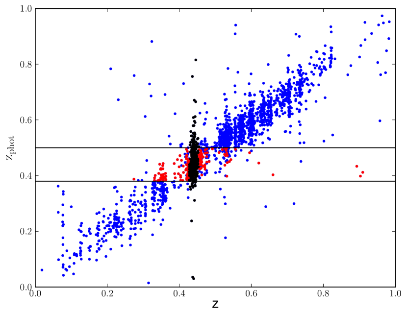
Figure 1: Photometric vs. spectroscopic redshifts for galaxies in the cluster field and in the magnitude range $\mathrm{18\,\leq\,R_{C}\,\leq\,24}$. Black dots represent spectroscopically confirmed members. The two horizontal lines indicate the $\mathrm{z_{phot}}$ range chosen for membership selection of the galaxies without z. Within this range only galaxies with chosen colors are selected as members. In this diagram these galaxies are indicated as red dots. Blue crosses are galaxies outside the spectroscopical and photometrical membership selections.

2.1 Estimation of stellar mass

Stellar masses of cluster member galaxies have been obtained, using the spectral energy distribution (SED) fitting technique performed by MAGPHYS (da Cunha et al. 2008), by setting all member galaxies to the mean cluster redshift. MAGPHYS uses a Bayesian approach to choose the template that best reproduces the observed galaxy SED. It is based on the stellar population synthesis models of either Bruzual & Charlot (2003) or Bruzual & Charlot (2007), with a Chabrier (2003) stellar initial mass function and a metallicity value in the range 0.02–2 $\mathrm{Z_{\odot}}$. The difference between the two libraries of models is in the treatment of the thermally pulsating asymptotic giant branch stellar phase, which affects the NIR emission of stellar populations with an age of $\mathrm{\sim}$ 1 Gyr. There is still considerable ongoing discussion on the way to model this phase of stellar evolution (Maraston et al. 2006; Kriek et al. 2010). We therefore tried adopting both libraries and found no significant difference (on average) in the stellar mass estimates. For simplicity, in the rest of the paper we report results based only on the more traditional library of models of Bruzual & Charlot (2003).

The spectral energy distribution is then obtained considering the history of the star formation rate (SFR) parametrized as a continuum model, $\mathrm{SFR\propto e^{-\gamma t}}$, with superimposed random bursts. The timescale $\mathrm{\gamma}$ is distributed according to the probability density function $\mathrm{p(\gamma)=1\,-\,\tanh(8\gamma\,-\,6)}$, which is uniform between 0 and 0.6 $\mathrm{Gyr^{-1}}$ and drops exponentially to zero at 1 $\mathrm{Gyr^{-1}}$. In this model, the age of the galaxy is a free parameter uniformly distributed over the interval from 0.1 to at most 13.5 Gyr. However, an upper limit for this value is provided by the age of the universe at the considered redshift.

For each galaxy model MAGPHYS produces both the dust free and the attenuated spectrum. The attenuated spectra are obtained using the dust model of Charlot & Fall (2000). The main parameter of this model is the total effective V-band absorption optical depth of the dust as seen by young stars inside birth clouds, $\mathrm{\widehat{\tau_{V}}}$. This parameter is distributed according to a probability density function which is approximately uniform over the interval from 0 to 4 and drops exponentially to zero at $\mathrm{\widehat{\tau_{V}}}\,\sim\,6$.

As an output of the SED fitting procedure, MAGPHYS provides both the parameters of the best-fit model and the marginalized probability distribution of each parameter. We adopt the median value of the probability distribution as our fiducial estimate of a given parameter, with lower and upper limits provided by the 16% and 84% percentiles of the same distribution. Using these limits we find that the typical 1 $\sigma$ error on the $\rm{M}_{\star}$ estimates is $\sim 0.15$ dex.

We translate our completeness limit in magnitude, $\mathrm{R_{C}\,=\,24}$, to a completeness limit in mass, $\mathrm{10^{9.5}\,\rm{M}_{\odot}}$, based on the relation between these two quantities shown in Fig. 2. The completeness mass limit we choose is that for the passive galaxies population, which guarantees our sample is also complete for the population of SF galaxies since they are intrinsically less massive than passive galaxies at a given magnitude.

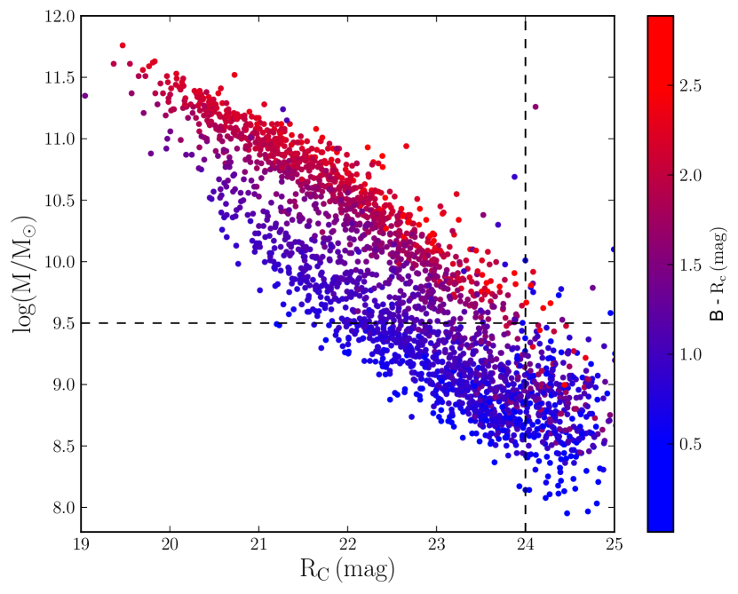
Figure 2: Galaxy stellar mass as function of $\mathrm{R_{C}}$ magnitude for cluster members. The points are color coded according to their $\mathrm{B\,-\,R_{C}}$ color. The vertical dashed line represents the completeness magnitude of our sample, and the horizontal dashed line represents the corresponding completeness mass.

In addition to $\rm{M}_{\star}$, among all the parameters provided by the MAGPHYS procedure, we also consider the specific star formation rate (i.e., star formation rate per unit mass, sSFR $\equiv$ SFR/$\rm{M}_{\star}$). The sSFR values are used to distinguish between SF and passive galaxies. Even if we do not expect the sSFR estimates from optical SED fitting to be very accurate, they are sufficiently good to allow identification of the well-known bimodality in the galaxy distribution (see Sect. 1). This can be better appreciated by looking at the sSFR distribution of cluster galaxies, shown in Fig. 3. This distribution is clearly bimodal. Following Lara-López et al. (2010, and references therein) we use the value sSFR$=10^{-10}$ yr^-1 to separate the populations of SF and passive galaxies. This value also corresponds to a local minimum in the sSFR distribution.

In the public MAGPHYS library, there are many more dusty and SF models than passive models (E. da Cunha, priv. comm.). Whenever an optical SED can be equally well fitted by a passive model and by a dusty SF model, the median solution is biased in favor of dusty SF models, since they occupy a larger area of the parameter space than passive models. It is therefore possible that some truly passive galaxies are classified as dusty SF galaxies. To estimate how serious this misclassification might be, we fit the sSFR distribution with two Gaussian distributions (see Fig. 3). We make the hypothesis that misclassified passive galaxies lie in the high-sSFR tail of the Gaussian centered at low sSFR. The fraction of the area occupied by this Gaussian at sSFR$>10^{-10}$ yr^-1 is 0.5%, and this is our estimate of the fraction of passive galaxies misclassified as SF. Similarly, one can estimate that the fraction of SF galaxies incorrectly classified as passive is 4%. Given that these fractions are small, we consider our sSFR estimates sufficiently good to separate our sample into the two populations of passive and SF galaxies.

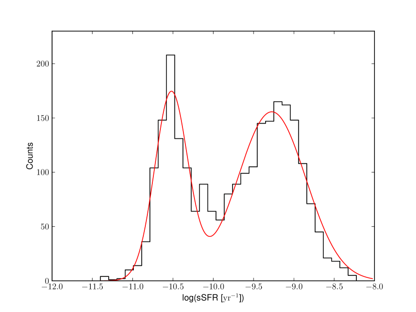
Figure 3: Distribution of the sSFR for the total sample of cluster galaxies. The red curve represents the best-fit to this distribution with two Gaussians.

In order to check the reliability of our $\rm{M}_{\star}$ estimates, we make use of the data from the UltraVista survey (McCracken et al. 2013) which is an ultra-deep, near-infrared survey with the VISTA survey telescope of the European Southern Observatory. From the UltraVista public catalog we select only ‘USE = 1’ objects, i.e., objects classified as galaxies, with a K magnitude above the detection limit of 23.9, and with uncontaminated and accurate photometry (Muzzin et al. 2013b). We select only galaxies with masses larger than our completeness limit ($\mathrm{10^{9.5}\,\rm{M}_{\odot}}$), and in the same photometric redshift range $\mathrm{0.38\,\leq\,z_{phot}\,\leq 0.50}$ used for our cluster membership selection – UltraVista $\mathrm{z_{phot}}$ have been obtained with the EAZY code of Brammer et al. (2008). To separate the UltraVista sample into the passive and SF populations we use the separations provided by Muzzin et al. (2013a) in the UVJ diagram.

We compare the masses provided in the UltraVista data-base (and obtained using the FAST SED-fitting code of Kriek et al., 2009) with those we obtained applying MAGPHYS on the UltraVista photometric catalog, using all of the available 30 bands, which cover the ultraviolet to mid-infrared, $\mathrm{24\,\mu m}$, spectral range. We find a good agreement between the two $\rm{M}_{\star}$ estimates, apart from a median shift $\mathrm{\Delta M\,=\,\log(M/\rm{M}_{\odot})_{MAGPHYS}\,-\,\log(M/\rm{M}_{\odot})_{FAST}\,=\,-0.07}$ independent from the galaxy type and mass. This comparison suggests that the $\rm{M}_{\star}$ estimates are not strongly dependent on the adopted SED-fitting algorithm, since the mass difference is well below the typical uncertainty in the individual $\rm{M}_{\star}$ estimates.

We then use the UltraVista dataset to check the effect of using only the optical bands in the SED fitting. In fact, for our analysis of the cluster SMF we can only use the optical SUBARU bands (BVriz) over the whole cluster field. For this test, we apply MAGPHYS to the selected UltraVISTA dataset once using all available bands, and another time using only the five optical SUBARU bands. The $\rm{M}_{\star}$ estimates obtained using optical bands only are systematically higher than those obtained using all available bands, particularly for the passive galaxies. The median value of the shift, $\mathrm{\Delta M\,=\,log(M/\rm{M}_{\odot})_{all\,bands}\,-\,log(M/\rm{M}_{\odot})_{optical}}$, is -0.07 for SF galaxies and -0.23 for passive galaxies. The shift for the SF galaxies is small, well below the typical uncertainty in individual $\rm{M}_{\star}$ estimates. On the other hand, the shift in mass for the passive galaxies is not negligible.

The reason for the systematic shift in the $\rm{M}_{\star}$ estimates of passive galaxies is probably related to the fact that MAGPHYS, when run on its public library, tends to favor dusty SF models rather than passive modes, when they cannot be distinguished based on the available data. We therefore run MAGPHYS again only on the sample of passive galaxies, this time using a library of templates heavily biased to fit old stellar populations with very little star formation (kindly provided by E. da Cunha). Using this library, we find that the shift between the masses estimated using all UltraVISTA bands, and those estimated using only optical bands is reduced to -0.13. Since this is within the typical uncertainty in individual $\rm{M}_{\star}$ estimates, we consider the new mass estimates to be acceptable.

Using this new library of passive models, we then redetermine the stellar masses of the passive galaxies identified in the cluster M1206, by running MAGPHYS again.

2.2 Completeness and membership corrections

To determine the cluster SMF, we need to apply two corrections to the observed galaxy counts. One is the correction for the incompleteness of the sample of galaxies with $\mathrm{z_{phot}}$, which also contains all the galaxies in the spectroscopic sample. The second correction is to account for interlopers in the sample of photometrically selected members (their presence is evident from Fig. 1, note the red dots with z very different from the cluster mean z).

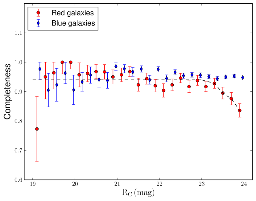
Figure 4: Completeness of the $\mathrm{z_{phot}}$ sample as a function of the $\mathrm{R_{C}}$ magnitude, separately for red ($\mathrm{B\,-\,R_{C}}\geq 1.5$, red dots) and blue ($\mathrm{B\,-\,R_{C}}<1.5$, blue diamonds) galaxies. The dashed line represents the adopted completeness as a function of $\mathrm{R_{C}}$ for the sample of passive members, and, down to $\mathrm{R_{C}}=23$, for the sample of SF members also. For $\mathrm{R_{C}}>23$, we adopt the same completeness used for brighter SF members.

We estimate the completeness, C, of the sample of galaxies with $\mathrm{z_{phot}}$ by measuring the ratio between the number of galaxies with $\mathrm{z_{phot}}$, $\mathrm{N_{zp}}$, and the number of galaxies in the $\mathrm{R_{C}}$ photometric sample, $\mathrm{N_{p}}$, C $\equiv\mathrm{N_{zp}/N_{p}}$. In Fig. 4, we show this completeness in different magnitude bins, for red and blue galaxies separately, where we use a color $\mathrm{B\,-\,R_{C}}=1.5$ to separate the two samples. This value corresponds to the sSFR value used to separate passive and SF members (see Sect. 2.1), and can therefore be used as a proxy for distinguishing these two populations when sSFR estimates are not available. In fact, sufficient photometric information is not available for all of the $\mathrm{N_{p}}$ galaxies to allow for a reliable sSFR estimate to be obtained from SED fitting.

Completeness is $>90$% down to $\mathrm{R_{C}\,=}$ 23. In this magnitude range the variation of C with $\mathrm{R_{C}}$ is negligible and C is not significantly different for the red and blue samples. We therefore adopt the value C= 0.94. In the magnitude range $\mathrm{23\,\leq R_{C}\,\leq 24}$, we adopt the same C value for the sample of SF galaxies, while for the passive galaxies we apply a magnitude-dependent correction (using the values shown by the red dots in Fig. 4). We do not consider galaxies with $\mathrm{R_{C}\,>}$ 24 in our analysis; on average in our sample this magnitude limit corresponds to $\rm{M}_{\star}<\mathrm{10^{9.5}\,\rm{M}_{\odot}}$ (see Fig. 2). Down to this limiting $\rm{M}_{\star}$ there are 1363 cluster members, of which 462 are spectroscopically confirmed (i.e., $\sim 1/3$ of the total). We define the correction factor for incompleteness as $\mathrm{f_{C}}=\mathrm{1/C}$.

As for the membership correction of the $\mathrm{z_{phot}}$ sample, we follow the approach of van der Burg et al. (2013). We define the purity, P, of the sample of photometric members as the ratio between the number of photometric members that are also spectroscopic members, and the number of photometric members with z, $\mathrm{P}=\mathrm{N_{pm\,\cap\,zm}}/\mathrm{N_{pm\,\cap\,z}}$. Since some real members are excluded by the $\mathrm{z_{phot}}$ and color membership selection, we need to define another completeness, given by the ratio between the number of spectroscopic members that are also photometric members and the number of spectroscopic members $\mathrm{C_{M}}=\mathrm{N_{pm\,\cap\,zm}}/\mathrm{N_{zm}}$. The membership correction factor of the $\mathrm{z_{phot}}$ sample is then given by $\mathrm{f_{M}}\equiv\mathrm{P/C_{M}}$. There is no significant dependence of $\mathrm{f_{M}}$ from the galaxy $\rm{M}_{\star}$ (see Fig. 5, left panel), but it does depend mildly on projected clustercentric distance, R (see Fig. 5, right panel). This dependence is similar for passive and SF galaxies, so we adopt the one evaluated for the passive sample also for the SF sample.

Note that the completeness correction factor $\mathrm{f_{C}}$ applies to the full sample of photometric and spectroscopic members, since the sample of galaxies with z is a subset of the sample of galaxies with $\mathrm{z_{phot}}$, while the membership correction factor $\mathrm{f_{M}}$ only applies to the sample of photometric members, since the membership based on z is considered to be correct.

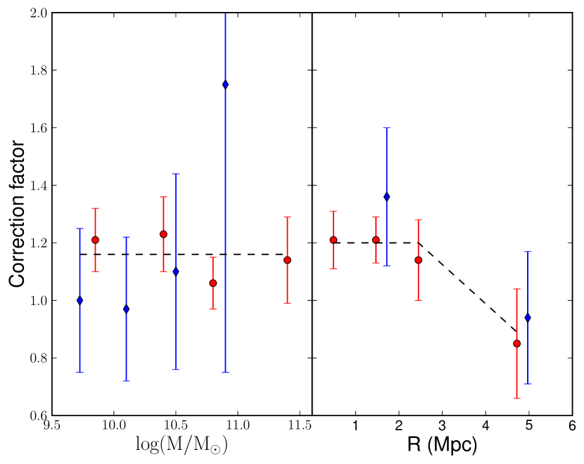
Figure 5: The membership correction factor $\mathrm{f_{M}}$ (see text) as a function of $\rm{M}_{\star}$ (left panel) and clustercentric radius R (right panel). We adopt a correction factor independent of $\rm{M}_{\star}$ and dependent on R, the same for the samples of passive (red dots) and SF (blue diamonds) members.

3 The stellar mass function

We derive the cluster SMF by counting the number of cluster members (defined in Sect. 2) per bin of $\rm{M}_{\star}$, and correcting these counts as described in Sect. 2.2. The resulting $\rm{M}_{\star}$ distribution is shown in Fig. 6 for all cluster members, and also, separately, for passive and SF cluster members. We estimate the errors in the galaxy counts with the bootstrap procedure (Efron and Tibshirani 1986).

We fit these SMFs with a Schechter (1976) function

$$\mathrm{\Phi(\log M)=\ln(10)\,\Phi^{*}\,\left(\frac{M}{M^{*}}\right)^{1+\alpha}\exp\left(-\frac{M}{M^{*}}\right)\,d(\log M),}$$ (1)

where $\mathrm{\Phi^{*}}$ is the normalization, $\mathrm{\alpha}$ is the low-mass end slope, and $\mathrm{M^{*}}$ corresponds to the exponential cutoff of the SMF at high masses. The fits are performed down to the mass limit $\mathrm{10^{9.5}\,M_{\odot}}$ (see Sect. 2.2), using the maximum likelihood technique (Malumuth & Kriss, 1986). This technique has the advantage that no binning of the data is required. The normalization $\mathrm{\Phi^{*}}$ is not a free parameter, since it is constrained by the requirement that the integral of the fitting function over the mass range covered by observations equals the number of galaxies in the sample. Of course, this number must be corrected for completeness and membership contamination. Therefore, in the maximum likelihood fitting procedure, the product of the completeness and membership correction factors, $\mathrm{f_{C}\cdot f_{M}}$, are used as weights for the individual values of $\rm{M}_{\star}$. Therefore, there are only two free parameters in the fit, $\mathrm{\alpha}$ and $\mathrm{M^{*}}$, except when we fit the data with a double Schechter function (in Sect. 3.1),

$$\mathrm{\Phi(\log M)=\ln(10)\,\Phi^{*}\,\times}$$

$$\mathrm{\left[\left(\frac{M}{M^{*}}\right)^{1+\alpha}\exp\left(-\frac{M}{M^{*}}\right)+f_{2}\left(\frac{M}{M_{2}^{*}}\right)^{1+\alpha_{2}}\exp\left(-\frac{M}{M_{2}^{*}}\right)\right]\,d(\log M).}$$ (2)

In this case there are three additional free parameters, $\mathrm{\alpha_{2}}$ and $\mathrm{M^{*}_{2}}$, and the ratio between the normalizations of the two Schechter functions, $\mathrm{f_{2}=\Phi^{*}_{2}/\Phi^{*}}$.

In the fits, in addition to the statistical errors, we also take into consideration the errors on the stellar mass estimates. These are evaluated by performing 100 Monte-Carlo simulations in which the mass of each galaxy is extracted randomly from a Gaussian distribution centered on the best-fit mass value, with a standard deviation equal to the error on the mass estimate. The errors on the stellar mass estimates provide only a minor contribution to the uncertainties on the best-fit Schechter function parameters, which are dominated by the statistical errors on the number counts.

We do not take the errors on the photometric completeness into account (see Fig. 4 in Sect. 2.2) since they are small. They would affect mostly the normalization of the SMF, while in most of our analyses we are only interested in comparing the shapes of different SMFs. We only care about the normalization of the SMF when comparing the passive and SF samples (Sect. 3.1) and when comparing the SMF in the central cluster region to the mass in the intracluster light (ICL, see Sect. 5). Also, in these cases, we estimate that the errors on the completeness can be neglected without a significant impact on our results.

The errors on the membership correction factor $\mathrm{f_{M}}$ (see Fig. 5 in Sect. 2.2) are significantly larger than those on the completeness. We estimate their effect on the stellar mass function in the following way. First, we consider the effect of adopting different values of $\mathrm{f_{M}}$ for red (passive) and blue (SF) galaxies, given by their different means, rather than adopting the same value for both populations. Second, in the regions where $\mathrm{f_{M}}$ deviate from a constant, i.e., at $\mathrm{R\,>\,r_{200}}$, we consider the effect of adopting the two extreme values of $\mathrm{f_{M}}$ given by $\mathrm{f_{M}\,\pm\,\sigma_{f_{M}}}$, where $\mathrm{\sigma_{f_{M}}}$ is the error in our estimate of $\mathrm{f_{M}}$ at $\mathrm{R\,>\,r_{200}}$. We find that all the results of the analyses presented in the following sections do not change significantly when changing the membership correction factors as described above. We therefore conclude that the uncertainties on $\mathrm{f_{M}}$ do not have a significant impact on our results. For the sake of clarity, in the following sections we only present the results based on our best estimates of $\mathrm{f_{M}}$, i.e., those given in Sect. 2.2.

We assess the statistical significance of the difference between any two SMFs both parametrically, by comparing the best-fit parameters of the Schechter function, and non parametrically, via a Kolmogorov-Smirnov (K-S) test (e.g., Press et al. 1993). We require a minimum of ten objects in a sample for a meaningful comparison.

The K-S test compares the cumulative distributions and therefore it is only sensitive to differences in the shapes of the distributions, not in their normalizations. However, in most of our analysis we are not interested in the normalization of the SMF, rather in its shape. There are only two points in our analysis where the normalization of the SMF is important. One is in the comparison of the passive and SF populations (see Sect. 3.1), since different relative normalizations affect the mass value at which the two SMFs cross each other – a useful parameter to constrain theoretical models (see Sect. 5). Another point is the estimate of the mass that could have been stripped from galaxies and gone into the mass of the ICL (see Sect. 5). In other parts of our analysis, differences in the SMF normalization just reflect rather obvious dependencies of the number densities of galaxies (of different types) on the environments where they are located, e.g., the cluster is denser than the field by definition, and this over-density is higher among the population of passive galaxies by virtue of the well-known morphology-density relation (Dressler 1980). For the comparison of the SMFs of a given cluster galaxy population in different environments, the K-S test is particularly appropriate. For the same reason, to highlight differences in the SMFs, we only compare the shape parameters of the Schechter function best-fits, $\mathrm{\alpha}$ and $\mathrm{M^{*}}$, and not the normalization parameter $\mathrm{\Phi^{*}}$.

Table 2: Best-fit Schechter function parameters

Galaxy type	$\mathrm{\Phi^{*}}$	$\mathrm{\alpha}$	$\mathrm{log(M^{*}/\rm{M}_{\odot})}$	$\mathrm{f_{2}}$	$\mathrm{\alpha_{2}}$	$\mathrm{log(M^{*}_{2}/\rm{M}_{\odot})}$
Passive	654	-0.38 $\mathrm{\pm}$ 0.06	10.96 $\mathrm{\pm}$ 0.04	–	–	–
SF	156	-1.22 $\mathrm{\pm}$ 0.10	10.68 $\mathrm{\pm}$ 0.09	–	–	–
All	751	-0.39 $\mathrm{\pm}$ 0.18	10.94 $\mathrm{\pm}$ 0.16	0.65 $\mathrm{\pm}$ 0.20	-0.51 $\mathrm{\pm}$ 0.33	9.93 $\mathrm{\pm}$ 0.35
All	541	-0.85 $\mathrm{\pm}$ 0.04	11.09 $\mathrm{\pm}$ 0.04	–	–	–

The parametric comparison naturally takes the completeness and membership corrections applied to the number counts into account. These corrections are also taken into account in the K-S tests, since we use the correction factors as weights in the evaluation of the cumulative distributions whose maximum difference is used in the test to evaluate the statistical significance of the null hypothesis.

3.1 Different galaxy types

In Fig. 6, we show the SMF of the passive, and separately, the SF galaxy populations along with their best-fitting Schechter functions. The best-fit $\mathrm{\alpha}$ and $\mathrm{M^{*}}$ parameters and their 1 $\sigma$ uncertainties, obtained by marginalizing over the other free parameter, are shown in Fig. 7 and listed in Table 2. When split into the two cluster populations of passive and SF galaxies, the SMF displays a strong, statistically significant dependence on galaxy type. In particular, the SMF of SF galaxies is increasing at the low-mass end, while the SMF of passive galaxies is decreasing. This difference is also confirmed by the K-S test, which gives a very low probability to the null hypothesis that the $\rm{M}_{\star}$ distribution of SF and passive galaxies are drawn from the same population (see Table 4).

This type-dependence of the SMF is not only valid in general for the whole cluster, but also in different cluster regions, identified by their clustercentric distance or by their local galaxy number density in Sect. 3.2.1 and 3.2.2 (see Table 4).

In Fig. 6, we also show the sum of the two Schechter functions that describe the SMFs of passive and SF galaxies. We have also performed a fit of a single Schechter function to the SMF of all cluster galaxies together; the best-fit parameters for this function are given in Table 2. According to the likelihood-ratio test (Meyer, 1975), the sum of the two Schechter functions provides a significantly better fit than the single Schechter function (with a probability of $>0.999$), after taking into account the difference in the number of free parameters (four vs. two).

We also fit the SMF of all galaxies with a double Schechter (eq. 2) and five free parameters, namely the $\mathrm{\alpha}$ and $\mathrm{M^{*}}$ of the two Schechter functions and their relative normalization. The best-fit parameters are listed in Table 2 along with their marginalized errors. The best-fit parameters of one of the two Schechter functions are very similar to those of the Schechter function that provides the best-fit to the SMF of passive galaxies. On the other hand, the best-fit parameters of the other Schechter function are very different from those of the Schechter function that provides the best-fit to the SMF of SF galaxies. This means that while the best-fit with a double Schechter is optimal from a statistical point of view, it fails to correctly describe one of the two components of the cluster galaxy sample, that of SF galaxies. This is probably because of the fact that the sample of cluster galaxies is largely dominated by passive galaxies over most of the mass range covered by our analysis, and so it is difficult to correctly identify the minority component, that of SF galaxies. As a matter of fact, the uncertainties on the best-fit parameters of the double Schechter function are rather large.

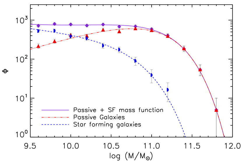
Figure 6: SMF for passive and SF cluster members (red triangles and blue demi-circles, respectively) and their best-fit Schechter functions (red triple-dot-dashed and blue dashed lines). The sum of the two SMFs is shown as a solid violet line. Violet diamonds are the counts obtained by considering all cluster members. The points represent counts in bins of 0.2 dex in $\rm{M}_{\star}$ divided for the bin size, and the counts have been corrected for completeness and membership. The (1 $\sigma$) errors on the counts have been estimated via the bootstrap resampling procedure.

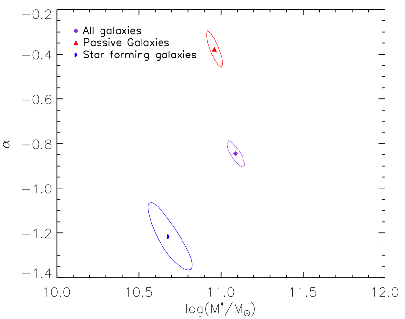
Figure 7: Best-fit Schechter parameters $\mathrm{M^{*}}$ and $\mathrm{\alpha}$ and 1 $\sigma$ likelihood contours.

Table 3: Best-fit Schechter function parameters for different environments

Galaxy type	Environment	$\mathrm{\alpha}$	$\mathrm{log(M^{*}/\rm{M}_{\odot})}$
SF	$\mathrm{R>r_{200}}$	-1.07 $\mathrm{\pm}$ 0.12	10.54 $\mathrm{\pm}$ 0.09
SF	$\mathrm{R\leq r_{200}}$	-1.52 $\mathrm{\pm}$ 0.17	11.16 $\mathrm{\pm}$ 0.37
Passive	$\mathrm{R>r_{200}}$	-0.43 $\mathrm{\pm}$ 0.09	10.99 $\mathrm{\pm}$ 0.05
Passive	$\mathrm{R\leq r_{200}}$	-0.40 $\mathrm{\pm}$ 0.08	11.00 $\mathrm{\pm}$ 0.05
Passive	Region 1	-0.15 $\mathrm{\pm}$ 0.15	10.92 $\mathrm{\pm}$ 0.08
Passive	Region 2	-0.54 $\mathrm{\pm}$ 0.14	10.97 $\mathrm{\pm}$ 0.10
Passive	Region 3	-0.44 $\mathrm{\pm}$ 0.15	10.99 $\mathrm{\pm}$ 0.10
Passive	Region 4	-0.57 $\mathrm{\pm}$ 0.14	11.09 $\mathrm{\pm}$ 0.11
Passive	Region (a)	-0.13 $\mathrm{\pm}$ 0.16	10.93 $\mathrm{\pm}$ 0.08
Passive	Region (b)	-0.55 $\mathrm{\pm}$ 0.16	11.00 $\mathrm{\pm}$ 0.12
Passive	Region (c)	-0.41 $\mathrm{\pm}$ 0.11	10.95 $\mathrm{\pm}$ 0.07
Passive	Region (d)	-0.35 $\mathrm{\pm}$ 0.09	10.96 $\mathrm{\pm}$ 0.06

Table 4: Results of the K-S tests

Compared samples	N1, N2	Prob. (%)
Type dependence
Passive vs. SF in the cluster	846, 517	$<0.01$
Passive vs. SF in Region 2	120, 021	$<0.01$
Passive vs. SF in Region 3	120, 031	$<0.01$
Passive vs. SF in Region 4	102, 020	$<0.01$
Passive vs. SF in Region (b)	096, 033	0.4
Passive vs. SF in Region (c)	199, 054	$<0.01$
Passive vs. SF in Region (d)	328, 420	$<0.01$
Environment dependence - SF galaxies
SF within and outside $\mathrm{r_{200}}$	078, 439	$>10$
SF in Regions 2 and 3	031, 031	$>10$
SF in Regions 3 and 4	031, 020	$>10$
SF in Regions (b) and (c)	033, 054	$>10$
SF in Regions (c) and (d)	054, 422	$>10$
Environment dependence - passive galaxies
Passive within and outside $\mathrm{r_{200}}$	438, 408	$>10$
Passive in Regions 1 and 2	120, 120	0.8
Passive in Regions 2 and 3	120, 102	$>10$
Passive in Regions 3 and 4	102, 096	$>10$
Passive in Regions (a) and (b)	100, 083	0.4
Passive in Regions (b) and (c)	083, 199	$>10$
Passive in Regions (c) and (d)	199, 328	2

3.2 Different environments

To search for possible environmental dependences of the SMF, we separate passive and SF galaxies in this analysis, to disentangle possible type-specific environmental dependences of the SMF from the well-known environmental dependence of the galaxy population (Dressler 1980; Baldry et al. 2008 and references therein).

We adopt two definitions of ‘environment’, one based on the distance from the cluster center, and another based on the local number density of cluster members. Of course, these definitions are not entirely independent, given the correlation between local density and radial distance (e.g. Whitmore et al., 1993). Using these two definitions we define nine cluster regions, five at different distances from the cluster center, (four within $\mathrm{r_{200}}$, labeled 1 to 4, and another one at $\mathrm{R>r_{200}}$, see Sect. 3.2.1) and another four at different local densities (labeled (a) to (d), see Sect. 3.2.2).

Our first definition of environment assumes circular symmetry, but the cluster is significantly elongated in the plane of the sky (Umetsu et al., 2012). However, this assumption is dropped in our other definition, as the regions (a) to (c) are elongated in the direction traced by the galaxy distribution (see Fig. 10), which is similar to the elongation direction of the brightest cluster galaxy (BCG) and of the total mass of the cluster as inferred from a weak lensing analysis by Umetsu et al. (2012, see their Figs. 1 and 11). As we show below, our results are essentially independent on which definition of environment we adopt, hence the assumption of circular symmetry does not seem to be critical.

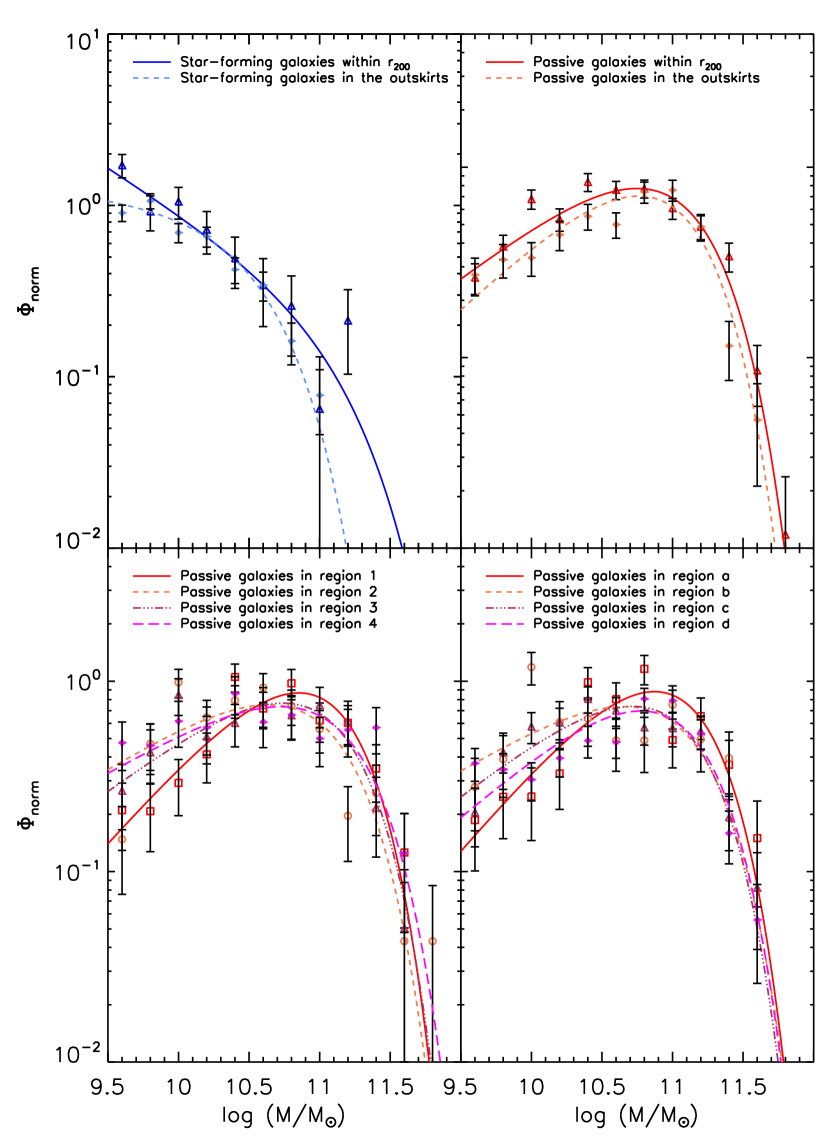
Figure 8: SMFs of SF and passive galaxies in different cluster regions and in the field. Upper left (resp. right) panel: SMFs of SF (resp. passive) cluster galaxies beyond and within $\mathrm{r_{200}}$. Bottom left panel: SMFs of passive cluster galaxies in four different regions, defined by their distances from the cluster center (see text). Bottom right panel: SMFs of passive cluster galaxies in four different regions, defined by their local number densities. SMFs are normalized to the total number of galaxies contained in the respective samples.

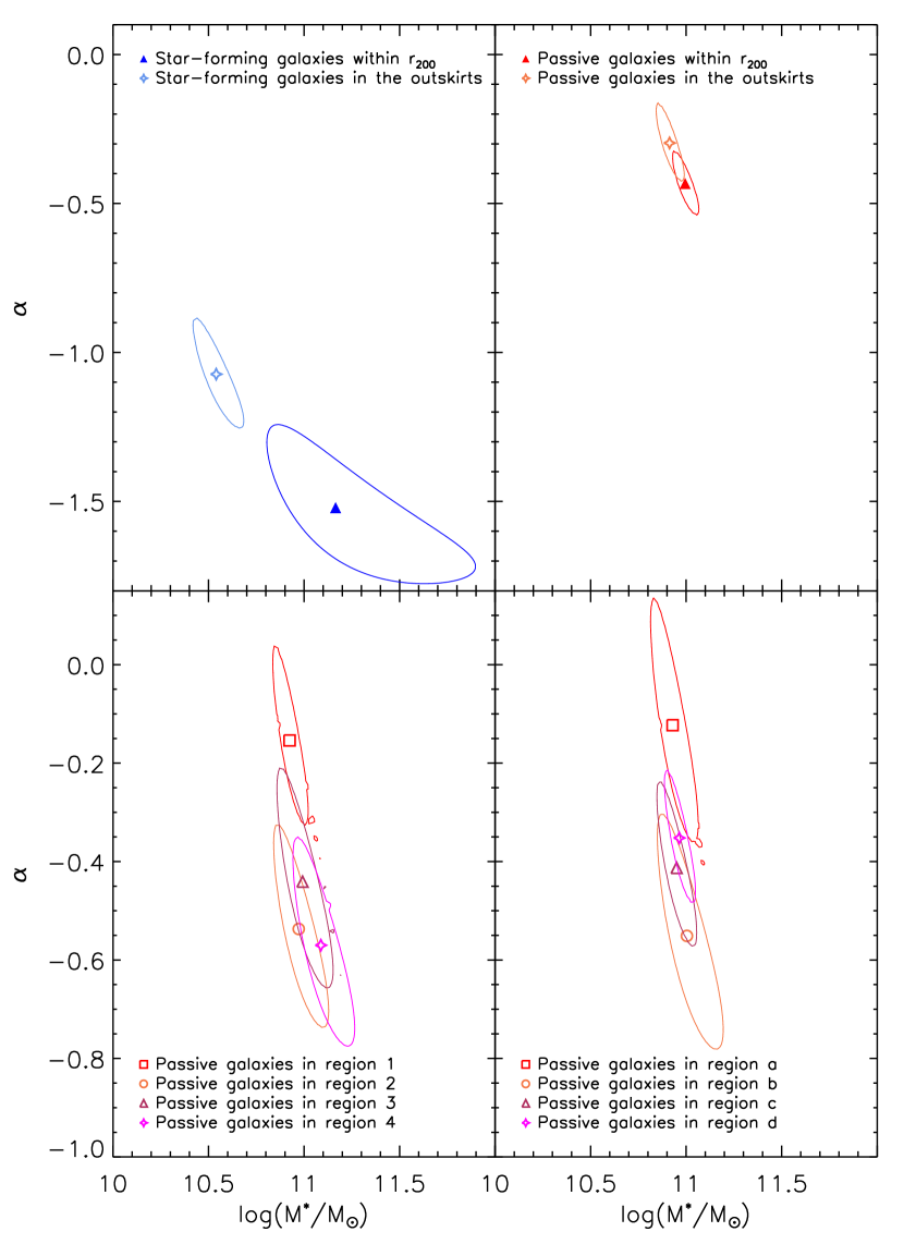
Figure 9: Best-fit Schechter parameters $\mathrm{M^{*}}$ and $\mathrm{\alpha}$ and 1 $\sigma$ likelihood contours, after marginalizing over the $\mathrm{\Phi^{*}}$ parameter for the SMFs of SF and passive galaxies in different cluster regions and in the field. The panels correspond one-to-one to those of Fig. 8.

3.2.1 Clustercentric radial dependence

We consider here the clustercentric distance as a definition of ‘environment’. The cluster center is identified with the position of the BCG (see Table 1 and Biviano et al., 2013).

We first consider the SMFs of passive and, separately, the SF cluster members, within and outside the virial radius, $\mathrm{r_{200}}$. These are shown in Fig. 8 (upper panels), and their best-fit Schechter function parameters are listed in Table 3 and shown in Fig. 9 (upper panels). The SMFs of cluster members within and outside the virial radius are not significantly different, neither for the passive nor for the SF galaxies. This is confirmed by the K-S test (see Table 4).

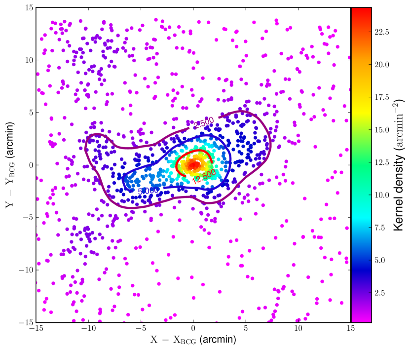
Figure 10: Spatial distribution of cluster members. The local number density is color coded as indicated by the bar at the right side of the plot. Coordinates are in arcmin with respect to the position of the BCG, see Table 1. Galaxies belonging to Regions (a), (b), (c), which are defined in Sect. 3.2.2, are those inside the red, blue, and purple solid lines, respectively. Galaxies belonging to Region (d) are the outer points.

We then determine the SMF in four different regions within $\mathrm{r_{200}}$, namely (see also Fig. 10):

1. $\mathrm{R/r_{200}\,\leq\,0.25}$.

2. $\mathrm{0.25\,<\,R/r_{200}\,\leq\,0.5}$.

3. $\mathrm{0.5\,<\,R/r_{200}\,\leq\,0.75}$.

4. $\mathrm{0.75\,<\,R/r_{200}\,\leq\,1}$.

The number of SF galaxies is not large enough to allow for Schecter function fits in all these regions, however, in some cases we have enough galaxies in the subsamples to allow for K-S test comparisons of the $\rm{M}_{\star}$ distributions. On the other hand, we have a sufficiently large number of passive galaxies to allow for meaningful Schechter function fits in all the four regions. The SMFs for the passive galaxies in the four different regions are shown in Fig. 8 (bottom left panel), along with their best-fitting Schechter functions. The best-fit parameters are listed in Table 3 and shown in Fig. 9 (bottom left panel).

To highlight a possible radial dependence of the cluster SMF we compare the $\rm{M}_{\star}$ distributions of cluster members in adjacent regions, using the K-S test, separately for SF and passive galaxies, whenever there are at least ten galaxies in each of the subsamples. The $\rm{M}_{\star}$ distributions of the SF cluster galaxies in the different regions are not statistically different (see Table 4). On the other hand, the K-S tests indicate a significant difference of the $\rm{M}_{\star}$ distributions of passive cluster members in Region 1 (the innermost one) and the adjacent Region 2. For no other adjacent regions does the K-S test highlight a significant difference from the SMFs of passive galaxies.

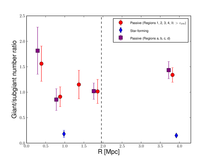
Figure 11: The number ratio of giant galaxies ($\mathrm{\log\rm{M}_{\star}/\rm{M}_{\odot}\geq 10.5}$) and subgiant galaxies ($\mathrm{\log\rm{M}_{\star}/\rm{M}_{\odot}<10.5}$), GSNR, for different samples of passive galaxies (red dots: Regions 1–4 and $\mathrm{R>r_{200}}$; magenta squares: Regions (a)–(d)) and SF galaxies (blue diamonds: within and outside the virial radius). For Regions (a)–(d) the point abscissae are set at the average clustercentric radii of the galaxies in the subsamples selected on the base of local density. The vertical dashed line indicates the location of $\mathrm{r_{200}}$.

From Fig. 9 (bottom left panel) and Table 3 one can see that the difference of the SMFs in Regions 1 and 2 is reflected in a difference in the values of the best-fit Schechter parameter $\alpha$. From Fig. 8 (bottom left panel) we can indeed see that the SMF of passive galaxies in Region 1 is characterized by a low-mass end drop that is more rapid than for the SMFs in other Regions.

From Fig. 9, one can notice that the SMFs of passive galaxies in Region 1 intersects those of passive galaxies in the other regions at $\mathrm{\log(\rm{M}_{\star}/\rm{M}_{\odot})\sim 10.5}$. Since these SMFs are normalized by the total number of galaxies in their respective samples, this does not mean that in Region 1 there are more galaxies with $\mathrm{\log(\rm{M}_{\star}/\rm{M}_{\odot})\sim 10.5}$ than in other regions. This mass value only indicates where the relative ratio of the number of galaxies more massive and less massive than a given value is maximally different for the SMF in Region 1 and in the other regions. We therefore use this value to separate ‘giant’ from ‘subgiant’ galaxies and plot the giant/subgiant number ratio (GSNR hereafter) as a function of radial distance from the cluster center in Fig. 11. Note that we use the correction factors defined in Sect. 2.2 as weights to compute the GSNR. The GSNR of passive galaxies decreases rapidly from the center (Region 1) to $\mathrm{R\sim 0.8}$ Mpc, then gently increases again toward the cluster outskirts ($\mathrm{R>3.5}$ Mpc) but without reaching the central value again. The GSNR of SF galaxies does not seem to depend on radius and is systematically below that of passive galaxies at all radii.

3.2.2 Density dependence

As an alternative definition of ‘environment’, we consider here the local number density of cluster members. This density is defined by smoothing the projected distribution of galaxies with a two-dimensional Gaussian filter in an iterative way. Initial estimates of the densities are obtained by using a fixed ‘optimal’ (in the sense of Silverman 1986) characteristic width for the Gaussian filter. In the second iteration, the characteristic width of the Gaussian filter is locally modified by inversely scaling the ‘optimal’ width with the square root of the initial density estimates. In other words, we adopt an adaptive-kernel filtering of the galaxy spatial distribution, where the kernel is adapted in such a way as to be narrower where the density is higher.

The distribution of cluster members is shown in Fig. 10, where symbols are colored according to the local galaxy density. We then define four regions of different mean projected density $\Sigma$ (in units of arcmin^-2):

1. $\mathrm{\Sigma>\,12.5}$.

2. $\mathrm{5<\,\Sigma\,\leq\,12.5}$.

3. $\mathrm{2.5<\,\Sigma\,\leq\,5}$.

4. $\mathrm{\Sigma\,\leq\,2.5}$.

From Fig. 10 one can note that Regions (a) and (b) approximately correspond to Regions 1 and 2 (defined in Sect. 3.2.1), while Region (c) corresponds roughly to Regions 3 and 4 with an extension beyond the virial radius. One obvious difference is that the regions defined by the value of $\mathrm{\Sigma}$ are more elongated than those defined by radius.

Since there are not enough SF galaxies to allow for meaningful Schechter fits to be performed in Regions (a) to (d), in Fig. 8 (bottom right panel) we only show the passive galaxy SMFs and their Schechter best fits. The best-fit parameters are listed in Table 3 and shown in Fig. 9 (bottom right panel).

The K-S tests indicate that the SMF of SF galaxies is independent of local density (see Table 4). On the contrary, the SMF of passive galaxies does depend on local density. In fact, the K-S tests performed between $\rm{M}_{\star}$ distributions in adjacent regions indicate a significant difference between Regions (a) and (b) (see Table 4). This difference is caused by the more rapid drop at the low-mass end of the SMF in Region (a) compared to the SMFs of other regions (Fig. 9, bottom right panel) and is reflected in a different value of the best-fitting parameter $\alpha$ (see Table 3).

In Fig. 11, we can see that the radial trend of the GSNR of passive galaxies found in regions 1–4 is confirmed when considering regions (a)–(d).

4 The stellar mass density profile

Using the sample of 1363 cluster members with $\rm{M}_{\star}\geq\mathrm{10^{9.5}\,M_{\odot}}$, we determine the radial profiles of number and stellar mass density of our cluster, N(R) and $\mathrm{\Sigma_{\star}(R)}$, respectively. We fit these profiles in the region $0.05<\mathrm{R/r_{200}}\leq 1$ (i.e., excluding the BCG) with a projected NFW (pNFW) model (Navarro et al., 1997; Bartelmann, 1996) using a weighted maximum likelihood fitting technique. For the determination of N(R), we use as weights those already used for the construction of the SMF, i.e., the product $\mathrm{f_{C}\cdot f_{M}}$ (see Sect. 2.2). For the determination of $\mathrm{\Sigma_{\star}(R)}$, we use the same weights multiplied by the galaxy stellar masses, $\mathrm{f_{C}\cdot f_{M}\cdot\rm{M}_{\star}}$. In Table 5, we list the values of the scale radii, $\mathrm{r_{s}}$, of the best-fit models. Note that our best-fit value for the $\mathrm{r_{s}}$ of N(R) is consistent with that estimated by (Biviano et al., 2013) on a slightly different sample. We find that $\mathrm{\Sigma_{\star}(R)}$ is significantly more concentrated than N(R).

The two profiles and their best-fit models are shown in Fig. 12. The error bars in the figure have been estimated via a bootstrap procedure. The pNFW model provides a good fit to the number density profile (reduced $\chi^{2}=1.4$), and a slightly worse fit to the stellar mass density profile (reduced $\chi^{2}=2.2$).

Table 5: The NFW scale radii of the density profiles

Profile	$\mathrm{r_{s}}$ (Mpc)
Galaxy number density	$0.80_{-0.14}^{+0.05}$
Stellar mass density	$0.52_{-0.07}^{+0.06}$
Total mass density	$0.34_{-0.06}^{+0.06}$

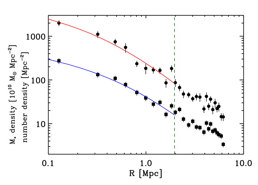
Figure 12: The stellar mass density profile (dots) and the number density profile (squares) and their best-fit projected NFW models (red and blue curves). The 1 $\sigma$ errors are shown, and evaluated using a bootstrap procedure. Both densities are space densities. The vertical dashed green line indicates the location of $\mathrm{r_{200}}$.

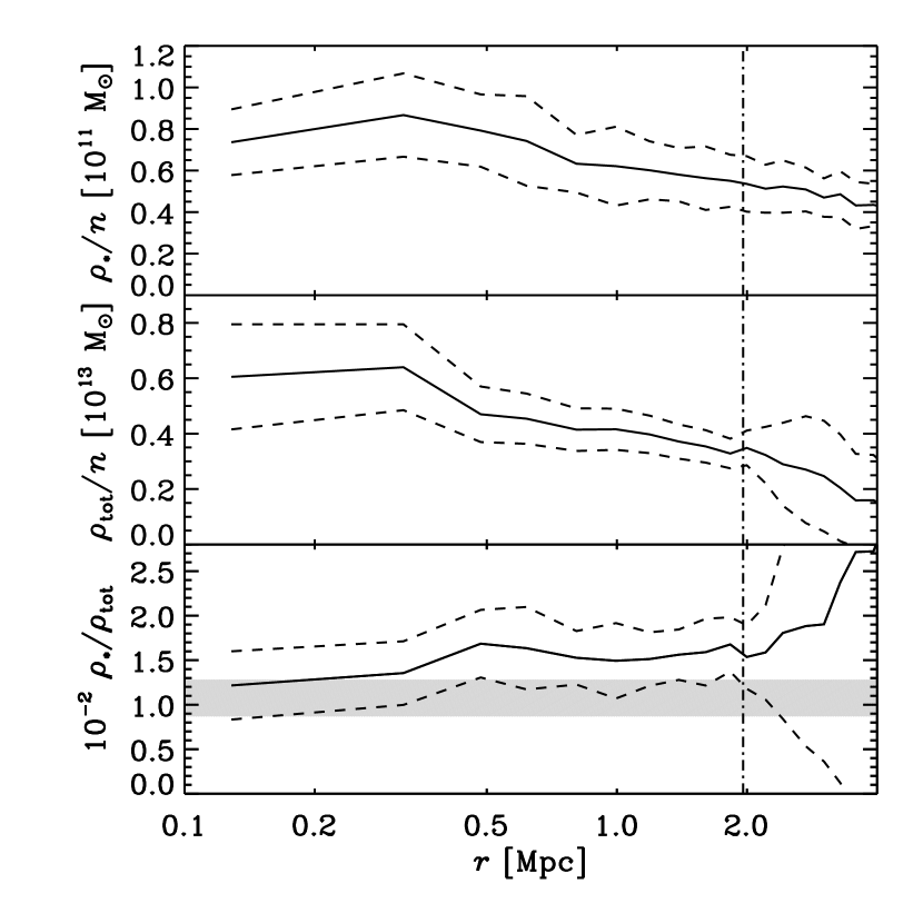
Figure 13: Top panel: the ratio of the stellar mass density and number density profiles. Middle panel: the ratio of the total mass density and number density profiles. Bottom panel: the ratio of the stellar mass density and total mass density profiles. Dashed lines indicate 1 $\sigma$ confidence regions. All densities are volume densities. The vertical dash-dotted line indicates the location of $\mathrm{r_{200}}$. The horizontal gray area indicates the cosmic value of the stellar mass fraction at the cluster mean redshift and its 1$\mathrm{\sigma}$ uncertainty.

We deproject the two density profiles using the Abel inversion, which assumes spherical symmetry (e.g. Binney & Tremaine, 1987). Before performing the numerical inversion, we smooth N(R) and $\mathrm{\Sigma_{\star}(R)}$ with the LOWESS technique (e.g. Gebhardt et al., 1994). The needed extrapolation to infinity is done as in Biviano et al. (2013, eq. 10). The deprojected stellar mass-to-number density profile ratio, $\mathrm{\rho_{\star}(r)/n(r)}$, is shown in the top panel of Fig. 13. The dashed lines represent 1 $\sigma$ confidence levels obtained by propagation of errors, where the fractional errors on the individual deprojected profiles are assumed to be those estimated for the projected profiles (Fig. 12). The ratio $\mathrm{\rho_{\star}/n}$ decreases by $\sim 30$% from the center to $\mathrm{r_{200}}$.

Both the relative concentration of the best-fit pNFW models of the two projected profiles and the ratio of the two deprojected profiles, indicate a mass segregation effect, i.e., galaxies are on average more massive (in stars) near the cluster center than at the cluster periphery. This is consistent with our finding that the GSNR is highest in the central cluster region (see Fig. 11).

We now consider the total mass density profile, $\mathrm{\rho_{tot}}$, as given by the gravitational lensing analysis of Umetsu et al. (2012). Specifically, we consider their NFW best-fit model parametrization of this profile. The ratios $\mathrm{\rho_{tot}/n}$ and $\mathrm{\rho_{\star}/\rho_{tot}}$ as a function of the 3D distance from the cluster center, r, are shown in the middle and bottom panels of Fig. 13. The distribution of total mass is more concentrated than both the distribution of galaxies (see also Biviano et al., 2013) and (but less significantly so) the distribution of stellar mass, the ratio of the stellar-to-total mass density increasing by $\sim 20$% from the center to $\mathrm{r_{200}}$. In other terms, the stellar mass fraction does depend on radius, but this dependence is not strong. This is consistent with the fact that the best-fit NFW model scale radius for the total mass density profile is only marginally different from that of the stellar mass density profile (see Table 5).

The median value of $\mathrm{\rho_{\star}/\rho_{tot}}$ within $\mathrm{r_{200}}$ is slightly higher (but not significantly so) than the (physical, not comoving) cosmic value of $0.011\pm 0.002$ at the cluster mean redshift, evaluated using the stellar mass density values of Muzzin et al. (2013a, their Table 2) and our adopted cosmological value for $\mathrm{\Omega_{M}}$.

5 Discussion

We find a very strong dependence of the cluster SMF on the galaxy type. This dependence is found in the whole cluster, as well as in different cluster regions defined by their clustercentric distance or by their local galaxy density. This dependence has been found previously in several studies (e.g. Bolzonella et al., 2010). The sum of the passive and SF SMFs gives rise to a SMF that deviates from a simple Schechter beyond the $\rm{M}_{\star}$ value where the two type SMFs cross each other (see Fig.13 in Peng et al., 2010). Indeed, we find that the fit of the SMF of all galaxies by the sum of the two best-fit Schechter functions of the passive and SF populations, is significantly better than the fit by a single Schechter.

The phenomenological model of Peng et al. (2010, well described in Baldry et al. 2012) has interpreted the double Schechter function shape of the galaxy SMF in terms of ‘mass quenching’ and ‘environmental quenching’, which transform star-forming (SF) galaxies into passive. If a galaxy sSFR is independent of mass and the probability of ‘mass quenching’ is proportional to SFR, then the Schechter SMF of SF galaxies transforms into a steeper single Schechter SMF of passive (quenched) galaxies. Environmental quenching is supposed to be independent of mass, so it does not affect the overall shape of the SMF, but only its normalization, as SF (blue) galaxies are turned into passive (red) galaxies. The passive SMF appears as the combination of the single Schechter function originating from mass quenching and of another Schechter function originating from environmental quenching. This bimodality should be particularly apparent in high-density regions where the environmental quenching is most effective. Post-quenching mergers can then change the shape of the passive SMF by increasing the number of very massive galaxies relative to the less massive galaxies.

This model makes specific predictions about the general evolution of the SMFs of SF and passive galaxies, which compare well with observations (Kauffmann et al., 2004; Bundy et al., 2005; Scoville et al., 2007; Drory & Alvarez, 2008; Scodeggio et al., 2009; Ilbert et al., 2010, 2013; Huang et al., 2013; Moustakas et al., 2013). The model also predicts the differential evolution of the relative number density of passive and SF galaxies in different environments, which is supported by observations (Bolzonella et al., 2010; Pozzetti et al., 2010). A consequence of the evolutionary model of Peng et al. (2010) is that the SMF for passive galaxies should be environment dependent. Such a dependence is visible in a local sample of galaxies (based on SDSS data, Peng et al. 2010), but not at higher redshift, apart from a slightly higher density of massive galaxies in denser regions (Bolzonella et al. 2010). That the predicted dependence is not observed at high redshifts could be because of the characteristics of the used samples, which are generally not complete at low-masses.

At the redshift of M1206 (z=0.44), the model of Peng et al. (2010) predicts that the SMFs of passive and SF galaxies should cross at $\mathrm{\log\rm{M}_{\star}/\rm{M}_{\odot}\approx 10.1}$ in dense environments, which is the value we find for the SMF of M1206 (see Fig. 6). This value depends on the environment; we find the crossing mass is $\mathrm{\log\rm{M}_{\star}/\rm{M}_{\odot}\approx 10.5}$ (resp. 9.5) for the SMF of galaxies outside (resp. within) $\mathrm{r_{200}}$, and smaller than that found in the field by Muzzin et al. (2013a, see their Fig.10). Hence, we confirm the prediction of Peng et al. (2010) that the value above which passive galaxies dominate the SMF shifts to lower masses in denser regions.

We find that the shape of the SMF of SF galaxies does not depend on the environment, although we cannot examine it within the densest cluster region for lack of statistics. This is also in line with predictions from the model of Peng et al. (2010), and with other observations of field galaxy SMFs (e.g. Ilbert et al., 2010; Huang et al., 2013).

We also find little or no evidence of an environmental dependence of the shape of the SMF of passive galaxies outside the very central (densest) region. Peng et al. (2010) do predict an environmental dependence and present evidence for it in a sample drawn from SDSS data, but other analyses have failed to detect such a dependence (e.g. Vulcani et al., 2012, 2013). Balogh et al. (2001) have found the SMF of passive galaxies to be steeper in clusters than in the field, as expected if mass quenching occurs earlier in denser environments at a given mass (Peng et al., 2010), but Giodini et al. (2012) have found that the the SMF of passive galaxies is steeper in the field than in groups of galaxies.
We do find a very significant change in the SMF of passive cluster galaxies in the very inner (and densest) region, $\mathrm{R\leq 0.25\,r_{200}}$, corresponding to $\simeq 0.5$ Mpc (see Fig. 8, bottom left panel). This change corresponds to a very steep radial decrease in the number ratio of giant ($\mathrm{\rm{M}_{\star}/\rm{M}_{\odot}\geq 10^{10.5}}$) to subgiant ($\mathrm{10^{9.5}\leq\rm{M}_{\star}/\rm{M}_{\odot}<10^{10.5}}$) galaxies (GSNR; see Fig. 11), from the center to $\sim 0.8$ Mpc. Beyond this radius the GSNR increases but more gently toward the cluster outskirts. The GSNR of SF galaxies does not show a significant radial dependence, but the innermost region is not sampled by our data, for lack of a statistical significant number of SF galaxies.

Our definition of ‘subgiants’ is close to the definition of ‘dwarfs’ used by Sánchez-Janssen et al. (2008), i.e., galaxies 1.0 mag fainter than the characteristic magnitude in the $r$-band luminosity function. Their magnitude cut roughly corresponds to $\rm{M}_{\star}\sim 10^{10.5}\rm{M}_{\odot}$. Using a large number of nearby clusters they find a clear increasing trend in the dwarf/giant number ratio with clustercentric radius, out to $\sim 2\,\mathrm{r_{200}}$, and they find this trend to be due to blue galaxies, while no trend is found for the red galaxies. Their results are therefore completely at odds with ours. Since the cluster sample analyzed by Sánchez-Janssen et al. (2008) is at $\mathrm{z<0.1}$, this difference seems to suggest a rapid evolution of the GSNR, different for the different populations of cluster galaxies. Quenching will transform the SF galaxies in M1206 into passive galaxies, which could flatten the dependence of the passive GSNR with radius (see Fig. 11), making it more similar to the GSNR observed by Sánchez-Janssen et al. (2008) for red galaxies. It is however more difficult to suggest a scenario for why the GSNR of blue/SF galaxies should grow a radial dependence with time.

Our results appear more consistent with the findings of Popesso et al. (2006) and Barkhouse et al. (2009). Popesso et al. (2006) find a lack of dwarf, red galaxies in the central cluster regions, and Barkhouse et al. (2009) find an increase in the number ratio of dwarf to giant red galaxies with clustercentric radius. In both studies there is no radial trend of the blue dwarf/giant ratio. The comparison with our results is not straightforward, however, as both studies are based on the analysis of luminosity rather than mass functions. Moreover, our definition of ‘subgiants’ differ from their definition of ‘dwarfs’. In Barkhouse et al. (2009) dwarfs are galaxies that are 2.8 mag fainter than the characteristic magnitude in the $\mathrm{R_{C}}$-band luminosity function, i.e., 1.12 dex below the value of $\mathrm{M^{*}}$ in our SMF, or $\rm{M}_{\star}\sim 10^{9.8}\rm{M}_{\odot}$. This limit is too close to the completeness limit of our sample and we cannot adopt it as the separation value to distinguish giant from subgiant (or dwarf) galaxies.

An interpretation of our GSNR trends can be given in terms of a scenario involving the processes of ram-pressure stripping (Gunn & Gott, 1972), harassment (Moore et al., 1996, 1998), and tidal destruction (Merritt, 1984). Ram-pressure stripping is the process that removes a galaxy gas as it moves through the intracluster medium. Harassment is the cumulative effect of multiple galaxy encounters and is able to transform a spiral galaxy into a spheroidal galaxy. Both processes are more effective in the denser, more central regions of a cluster. Tidal destruction is caused by the cluster gravitational field and is effective only very close to the cluster center (e.g. Moran et al., 2007). As a SF galaxy approaches the cluster center it is transformed into a passive galaxy by harassment and ram pressure. The SF galaxies are on average less massive than passive galaxies, and in addition, their masses may become even smaller as they are transformed to passive galaxies, e.g., by harassment. As a result, the number of passive galaxies increases with time especially at the low-mass end, and particularly so in the denser cluster regions where the transformation processes are more effective. This creates a decreasing trend of the passive galaxy GSNR from the cluster outskirts to its center. However, this trend might be reversed at very small radii because tidal mass stripping become so effective there that the low-mass galaxies are either totally destroyed or mass-stripped below the completeness limit of a given survey ($\mathrm{10^{9.5}\rm{M}_{\odot}}$ in our case).

A detailed and perhaps dedicated analysis of semi-analytical models in the context of cosmological numerical simulations would be required to (dis)prove this scenario, and this is beyond the scope of this paper. We can however refer to the simulation work of Conselice (2002) where the value $\alpha$ of the luminosity function of cluster galaxies is first shown to increase (in absolute values) and then decrease, as the number of interactions among galaxies increases. The initial increase is due to tidal stripping, until the stripping becomes so strong that stripped galaxies drop off the completeness limit of the given survey. We do observe the same non monotonous trend of $\alpha$ with local galaxy density (see Sect. 3.2.2).

Further support to our scenario comes from the comparison of the amount of mass in the ICL and of the mass that is missing from subgiant galaxies in the SMF of the innermost region. To estimate the amount of mass that could have been stripped from subgiant galaxies we proceed as follows. First, we calculate the total mass in the SMF of passive galaxies in the innermost Region 1 (see Sect. 3.2.1) in the mass range between $\mathrm{10^{9.5}-10^{10.5}\,\rm{M}_{\odot}}$,

$$\mathrm{M_{sub}}\equiv\int_{10^{9.5}\,M_{\odot}}^{10^{10.5}\,M_{\odot}}\mathrm{m\,\Phi(m)\,dm\,.}$$ (3)

The SMF of Region 1 shown in Fig. 8 has been normalized to the total number of galaxies contained in the subsample. In eq. 3 we use the non normalized SMF, with $\mathrm{\Phi^{*}=121}$. The lower limit of the integral corresponds to our completeness limit. The upper limit of the integral corresponds to the mass value where the normalized SMF of Region 1 intersects the normalized SMF of the adjacent Region 2 (see Fig. 8, bottom left panel). We have chosen this mass value also to separate giant from subgiant galaxies. We then recompute the integral in Eq. 3 by keeping the $\mathrm{\Phi^{*}}$ and $\mathrm{M^{*}}$ values of the SMF of Region 1 and by changing the slope to the best-fit value found for the SMF in the adjacent Region 2 (see Table 3). The difference between the two values of $\mathrm{M_{sub}}$ thus obtained is a measure of how much mass is missing in the subgiant mass range in Region 1 with respect to Region 2. We estimate the uncertainty on this difference by repeating this estimate with slopes fixed to the $\alpha\pm\mathrm{d}\alpha$ values of Region 2, where $\mathrm{d}\alpha$ is the error on $\alpha$ (see Table 3). The value we find, $\mathrm{\mathrm{\Delta M_{sub}=5.8_{-2.9}^{+3.3}\times 10^{11}\,\rm{M}_{\odot}}}$, can be compared with the estimate of ICL stellar mass in M1206, $\mathrm{9.9\pm 3.8\times 10^{11}\,\rm{M}_{\odot}}$ (Presotto et al., 2014). These two values are consistent within $\mathrm{\sim 1\,\sigma}$, within their admittedly large uncertainties. Our estimate would not change by more than 30% if we would extrapolate the integral of eq. 3 to very low masses, and in any case the dominant contribution to the ICL is expected to come from intermediate-to-high mass galaxies (Murante et al., 2007; Contini et al., 2014). This comparison is consistent with a scenario where the missing subgiant galaxies in the innermost cluster regions have lost part of their stellar mass into a diffuse intracluster component due to interactions with other cluster members or with the tidal cluster field. With a very similar approach Giallongo et al. (2014) come to the same conclusions about the nature of the ICL in another $\mathrm{z\sim 0.4}$ cluster.

The radial dependence of the GSNR is also reflected in the decreasing stellar mass-to-number density profile ratio (see Fig. 11). On average, among galaxies with $\rm{M}_{\star}\geq 10^{9.5}\rm{M}_{\odot}$ those near the cluster center are $\sim 30$% more massive than those near the cluster virial radius. This is not because of the presence of the central BCG, which was excluded from the analysis when we determined the density profiles. Our finding is consistent with the mild mass segregation found in groups by Ziparo et al. (2013), and with the mass segregation found in clusters at $\mathrm{z\sim 1}$ by van der Burg et al. (2013). In particular, the ratio of the best-fit concentrations of the stellar mass density and number density profile found by van der Burg et al. (2013), $1.4\pm 0.4$, is fully consistent with the ratio we find, $1.6\pm 0.4$. van der Burg et al. (2013) attribute this mass segregation to dynamical friction, which should have occurred before $\mathrm{z\sim 1}$, with little if any further evolution thereafter. However, mass segregation can also be the result of tidal stripping in the central cluster region, affecting galaxies in different ways depending on their mass. Since galaxies of lower mass galaxies are more affected by tidal stripping, they lose mass and drop off the completeness limit of $\mathrm{10^{9.5}\rm{M}_{\odot}}$ in our dataset.

To discriminate between dynamical friction and tidal stripping as the driving process of mass segregation in M1206, we turn our attention to the total mass density profile. We find that the total mass density profile is more concentrated than the galaxy number density profile, as already found by Biviano et al. (2013), as well as in many other clusters (e.g. Biviano & Girardi, 2003; Lin et al., 2004b; Biviano & Poggianti, 2009). We also find, however, that the total mass density profie is more concentrated than the stellar mass distribution, which is an entirely new result. Should dynamical friction be responsible for the observed mass segregation we would expect the total mass density profile to be less concentrated than the stellar mass density profile, as the diffuse dark matter component should gain energy at the expense of the subhalos (e.g. Del Popolo, 2012). Instead, we find the opposite. We therefore conclude that the observed mass segregation is not due to dynamical friction in M1206, but to tidal disruption of the less massive galaxies. Since most of the stellar mass is in the most massive galaxies, while most of the galaxies are low-mass galaxies, this process affects the number density profile much more severely than the stellar mass density profile.

The radial dependence of the stellar-to-total mass ratio is very mild. This mild dependence is consistent with the results of Biviano & Salucci (2006, see their Table 1), obtained using a sample of 59 nearby clusters (fully described in Biviano et al., 2002), and Bahcall & Kulier (2014, see their Fig.9), obtained using a sample of $\mathrm{z<0.3}$ clusters. Bahcall & Kulier (2014) find that the stellar mass fraction is roughly constant out to $\mathrm{\sim 40\,r_{200}}$. We confirm their result out to $\mathrm{\sim r_{200}}$; beyond that radius our error bars become very large (see Fig. 11). Their determination of the average cluster stellar mass fraction also agrees very well with the cosmic value, while our determination is consistent, but slightly above, the cosmic value.

6 Conclusions

We estimate the SMF and the stellar mass density profile, $\mathrm{\rho_{\star}(r)}$, of the $\mathrm{z=0.44}$ cluster M1206, using a sample of $\sim 1300$ cluster members, obtained in the CLASH-VLT program. Cluster membership has been evaluated using spectroscopic and photometric redshifts (for $\sim 1/3$ and $\sim 2/3$ of the members, resp.). Stellar masses are obtained by SED fitting with MAGPHYS (da Cunha et al. 2008). The SMF and $\mathrm{\rho_{\star}(r)}$ are corrected for incompleteness and contamination down to $\mathrm{\rm{M}_{\star}=10^{9.5}\rm{M}_{\odot}}$. Our main results are:

• The SMF of the cluster is significantly better fitted by a double Schechter function than by a single Schechter function. The SMFs of the passive and SF cluster populations are well fitted by single Schechter functions, with significantly different low-mass end slopes.

• The SMFs of passive and SF cluster members cross at $\mathrm{\rm{M}_{\star}/\rm{M}_{\odot}\simeq 10^{10.1}}$, in agreement with the prediction of the model of Peng et al. (2010). This crossing mass is higher in lower density regions.

• The shape of the SMF of SF galaxies is independent from the environment, as defined by either the local number density of galaxies, or the clustercentric radius, in the range $\sim 0.8-4.0$ Mpc (corresponding to $\sim 0.4-2.0\,\mathrm{r_{200}}$).

• The shape of the SMF of passive galaxies does depend on the environment, since the SMF decreases more steeply toward the low-mass end, in the innermost cluster region ($\leq 0.5$ Mpc) than in the other, more external regions.

• The number ratio of giant/subgiant galaxies is highest in the innermost region and lowest in the adjacent region ($0.5-1.0$ Mpc), then the ratio increases with radius toward the cluster outskirts.

• Both the number density and stellar mass density profiles can be fitted reasonably well by projected NFW models, but with different concentrations. The stellar mass density profile is significantly more concentrated than the number density profile and only slightly less concentrated than the total mass density profile.

• A possible interpretation of the environmental dependence of the SMF of passive galaxies and of the relative concentrations of the total, stellar mass, and number density profiles, is proposed in terms of tidal disruption of the less massive galaxies in the central cluster regions. On the other hand, dynamical friction seems not to be effective. Support for our interpretation comes from the comparison of the mass in the cluster ICL with the missing mass in the subgiant galaxy mass range in the innermost region.

In the future, we plan to extend our analysis of the SMF to the full set of CLASH-VLT clusters (Rosati et al. in prep.) and to test our scenario for the environmental dependence of the passive galaxy SMF with semi-analytical models within cosmological numerical simulations.