Periodic versus Intermittent Adaptive Cycles in Quasispecies Coevolution

Abstract

We study an abstract model for the coevolution between mutating viruses and the adaptive immune system. In sequence space, these two populations are localized around transiently dominant strains. Delocalization or error thresholds exhibit a novel interdependence because immune response is conditional on the viral attack. An evolutionary chase is induced by stochastic fluctuations and can occur via periodic or intermittent cycles. Using simulations and stochastic analysis, we show how the transition between these two dynamic regimes depends on mutation rate, immune response, and population size.

Evolution is commonly pictured as a dynamic process on a fitness landscape in sequence space. In general, this landscape depends not only on the genotype but varies dynamically as a function of the environment and coevolving interaction partners Wright1932 . Prominent biological examples are the coevolutionary dynamics between the adaptive immune system and virus populations such as HIV Nowak1990 ; Woo2012 or influenza Bedford2011 , or between bacteria and their phages Levin2013 . Continuous evolutionary innovations allow the virus to transiently escape immune suppression, triggering subsequent adaptations of the immune system. These dynamics can lead to coevolutionary cycles, which have been generally described in two different forms Woolhouse2002 ; Bedford2011 : either as an intermittent series of quasistationary states connected by stochastic jumps, or as periodic and largely deterministic oscillations. From a modeling perspective, this highly complex process is determined by three main features Perelson2002 . First, mutation rates are high and populations are large, which implies large genetic heterogeneity within the populations Domingo1985 . This has often been pictured in terms of broad quasispecies distributions around peaks in the fitness landscape Wang2006 ; Eigen1977 . At the same time, continuous adaption and coevolutionary arms races are driven by strong ecological interactions Woolhouse2002 ; Tellier2013 . These modulate effective fitness landscapes Gavrilets1998 ; Nowak1990 ; Arnoldt2012 and lead to nontrivial nonlinear population dynamics. Finally, stochastic effects in finite populations become especially pronounced whenever the first two issues are relevant at the same time Tsimring1996 ; Rouzine2001 ; Tellier2013 ; Gokhale2014 .

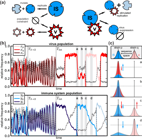
Figure 1: (a) Schematic model for the coevolutionary dynamics of virus (V) and immune system (IS). The two populations are subject to mutation and selection (left), but also to ecological interactions (right). (b) Exemplary trajectories of the relative frequencies of virulent strains $x_{i}$ (top) and corresponding antibodies $y_{i}$ (bottom). Regular oscillatory dynamics involving three strains turn into simpler two-strain oscillations at $T_{3\to 2}$ and finally transition into intermittency at $T_{\text{int}}$. Genetic variability within the populations is calculated from the average pairwise Hamming distance and indicated in gray dashed lines. (c) Sketch of the dynamics of the full population distributions in sequence space as described in the text.

Here, we offer a synthetic perspective on these processes. In our model [see Fig. 1(a)], we consider a population of $N$ viruses represented by their genotypes (binary sequences of length $L$ and frequency $x_{i}$) and replication rates $r_{i}=1$. A small number $n$ of these genotypes corresponding to particularly virulent strains have a fitness advantage $\alpha$ over the unit baseline, giving $r_{i}=1+\alpha$ for $i=p,q,\ldots$. Offspring sequences undergo mutations with per-base rate $\mu_{x}$. In the absence of immune suppression, and in the stationary state, the viral population localizes as so-called quasispecies around any of the fittest genotypes, provided the mutation rate is smaller than Eigen’s error threshold $\mu_{\text{c}}\approx\ln(\alpha+1)/L$ Eigen1977 . This simple picture is considerably complicated by the host’s adaptive immune system, which produces antibodies that recognize and neutralize viruses with matching epitopes Alberts2002 . Antibody production is specifically increased and variability in the binding affinity is introduced when viruses with matching genotype are encountered Rajewsky1996 , in a process that can be modeled in terms of mutation and selection. Similar concepts can be used for bacterial immune systems, where spacer sequences in the host genome complementary to genetic elements of a phage take antibodylike functions Levin2013 . Hence, for the immune system we introduce a second population of $N$ binary sequences with frequencies $y_{i}$, mutation rate $\mu_{y}$, unit replication rate for unstimulated production, and stimulated antibody production in the presence of perfectly matching viruses Kamp2002 ; Wang2006 . Ecological interactions then introduce frequency-dependent fitness terms $\propto x_{i}y_{i}$ for such matched virus and antibody pairs. Including these terms leads to a reduction of the viral load and stimulation of antibody production [Fig. 1(a), right]. In the deterministic limit ($N\to\infty$), our model is described by supplement

$$\begin{split}\dot{x}_{i}&=\textstyle{\sum_{j}}m^{x}_{ij}r_{j}x_{j}-\alpha x_{i}y_{i}-x_{i}\phi_{x},\\ \dot{y}_{i}&=\textstyle{\sum_{j}}m^{y}_{ij}(1+\gamma x_{j})y_{j}-y_{i}\phi_{y},\end{split}$$ (1)

where $i$ and $j$ run over all $2^{L}$ sequences. The fitness advantage $\alpha$ of virulent strains can be suppressed to background levels by a perfectly adapted immune system, which undergoes stimulated production at rate $\gamma$ when encountering matching viral epitopes. Further, $m^{x}_{ij}=\mu_{x}^{d_{ij}}(1-\mu_{x})^{L-d_{ij}}$ is the probability of having $d_{ij}$ simultaneous mutations, where $d_{ij}$ is the Hamming distance between $x_{i}$ and $x_{j}$. The dilution terms $\phi_{x/y}$ are obtained from the conditions $\sum_{i}\dot{x}_{i}=0$ and $\sum_{i}\dot{y}_{i}=0$, respectively, and keep the sizes of the two populations fluctuating around constant values. This constraint applies to the stationary phase of the adaptive race, while we ignore some of the effects of a changing viral load Nowak1990 ; Woo2012 ; Wang2006 ; Bull2007 and also neglect immune system memory Bianconi2010 and unspecific recognition Alberts2002 .

To facilitate a systematic study of the effects of demographic noise by means of simulations and theoretical analysis, our starting point is the underlying stochastic master equation supplement which has rarely been used in this context. Its deterministic limit leads to Eq. (1) and connects to established quasispecies theory Eigen1977 ; Kamp2002 . Exemplary simulation results obtained with the Gillespie algorithm Gillespie1992 are shown in Fig. 1(b), with parameters in the coexistence regime discussed below. We readily identify characteristics of the intermittent coevolutionary dynamics. First, a particularly virulent strain with its associated quasispecies “cloud” of mutants triggers a specific immune response (a), leading to a corresponding localization in the antibody sequence space (b). This gives alternative viral strains that are not under immune attack a fitness advantage, and after a brief “search” period during which the viral population becomes delocalized, this new fitness peak is colonized in a “growth” phase (c), awaiting the adaptive immune response (d). The delocalization and relocalization dynamics of each population in sequence space are clearly visible as transient increases in their respective mean pairwise Hamming distances [Fig. 1(b)]. Intriguingly, this sequence of events can occur both in the form of regular oscillations as well as by means of stochastically intermittent cycles Woolhouse2002 . The former occurs when the large genetic diversity within the population extends across the valleys between different fitness peaks and signifies periodic shifts in the extent to which these peaks are populated Gavrilets1998 . The latter case indicates that adaptation proceeds stochastically via the random discovery of previously unpopulated fitness peaks by relatively tightly localized populations.

Steady-state regimes: coexistence for mutation rates below interdependent error thresholds.

We use a reduced deterministic version of the model to determine stationary states and the associated error thresholds. We restrict the analysis to the populations of the $n$ virulent strains $x_{p,q,\ldots}$ and their respective antibodies $y_{p,q,\ldots}$, and lump all mutant sequences together in the so-called error tail Schuster1988 . The high-dimensional system (1) is then reduced to supplement

$$\begin{split}\dot{x}_{p}&=\left[Q_{x}\left(1+\alpha\right)-\alpha y_{p}-\bar{\phi}_{x}\right]x_{p},\\ \dot{y}_{p}&=\left[Q_{y}\left(1+\gamma x_{p}\right)-\bar{\phi}_{y}\right]y_{p},\end{split}$$ (2)

where $p$ runs over the $n$ strains which are coupled by the corresponding dilution terms $\bar{\phi}_{x/y}$. $Q_{x/y}=(1-\mu_{x/y})^{L}$ are the quality factors. A straightforward stability analysis of fixed points in this system with respect to $\mu_{x/y}$ as bifurcation parameters yields the phase diagrams of Fig. 2.

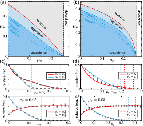
Figure 2: (a) Regimes of coevolution. High mutation rates $\mu_{x}$ of the virus lead to population delocalization, while for lower mutation rates a regime of coexistence emerges. Intermediate values lead to a degenerate localization regime for the virus (see text). (c) Steady-state values for relative frequencies $x_{p}=x_{q}$ and $y_{p}=y_{q}$ as a function of $\mu_{y}$ with $\mu_{x}=\mu_{y}$ (above) or $\mu_{x}=0.05$ (below). Solid lines are solutions of Eq. (2) and dots are simulation results. Panels (a) and (c) are for $\gamma=\alpha$, while (b) and (d) show analogous result for $\gamma=10\alpha$, where $L=8$, $n=2$, and $\alpha=10$.

As expected, we recover the classical result that the viral population localizes around a fitness peak only if $Q_{x}>Q_{c}\equiv\left(\alpha+1\right)^{-1}$, with increasing genetic variability (i.e., the width of the population distribution) for larger mutation rate $\mu_{x}$. However, antibodies are localized only (1) if their mutation rate $\mu_{y}$ is small enough, (2) if their production rate $\gamma$ is high enough and (3) if the virus attack is specific enough (i.e., tightly localized). These interdependent requirements are an inevitable consequence of ecological interactions, and they translate into the condition $Q_{y}=\left\{\left(\gamma/\alpha n\right)\left[Q_{x}(\alpha+1)-1\right]+1\right\}^{-1}$ as the analytical limit for the coexistence regime (blue dashed lines in Fig. 2). Only in this regime do we find the intriguing oscillatory dynamics shown in Fig. 1 that will be discussed below. Finally, in a somewhat model-specific “degenerate” regime bounded by $Q_{y}=\left\{\left(\gamma/\alpha\right)\left[Q_{x}(\alpha+1)-1\right]+1\right\}^{-1}$, the virus population can stably localize about several fitness peaks simultaneously such that none of these quasispecies is sufficiently tight to trigger a specific response of the immune system, which thus remains delocalized. The fixed points of the approximate system (2) coincide closely with the mean steady-state concentrations obtained by stochastic simulation of the full system (1) [see Figs. 2(c) and 2(d)]. Interestingly, for $\alpha=\gamma$ and symmetric mutation rates $\mu_{x,y}\equiv\mu$, the critical condition of coexistence can be approximated by $\mu\approx\left(1/2L\right)\ln\left(\alpha/2\right)$ for large $\alpha$ and $L$, which generalizes a comparable result for mutualistic frequency-dependent fitness Obermayer2009 to the case of antagonistic interactions. This correspondence also suggests that the error thresholds derived here should be largely unchanged if recognition between the two population tolerates some mismatches Obermayer2010 .

Noise-driven oscillations in the coexistence regime.

Performing a linear stability analysis in the coexistence regime reveals that the oscillations seen in the simulations are caused by $n-1$ pairs of purely imaginary eigenvalues. Numerical solutions of the deterministic Eqs. (2) show complex but regular oscillations involving all $n$ strains with slow amplitude variations controlled by higher-order nonlinearities (see Fig. S1 in the Supplemental Material supplement ). Results from stochastic simulations, however, suggest that such complex patterns quickly give rise to simpler oscillations involving only two strains, which at a later time transition into intermittency (cf. Fig. 1). Investigating the case $n>2$ by simulations below, we restrict further analysis to $n=2$. Also, here we only display more compact analytical results for the case $\gamma=\alpha$ (see the Supplemental Material supplement for general results). Our analysis exploits that in the coexistence regime mutation rates $\mu_{x/y}\lesssim\ln\alpha/L$ are small compared to the error thresholds and can be used as expansion parameters. To obtain the nonlinearities that control oscillation amplitudes, we expand Eq. (2) to first order and transform to polar normal form on the two-dimensional stable manifold supplement :

$$\dot{u} =-\frac{4}{5}L\left[\mu_{x}\left(\alpha+1\right)+\mu_{y}\right]u^{2},$$ (3a)

$$\dot{\varphi} =\frac{\alpha}{2}-\frac{L}{2}(\alpha+1)(\mu_{x}+\mu_{y})+\mathcal{O}(u),$$ (3b)

where $u$ is a squared radial coordinate indicating deviations from the coexistence fixed point and $\varphi$ measures the phase of the oscillations. Equation (3a) exhibits a weak geometric decay of the oscillation amplitude $\mathcal{O}(u^{2}\mu_{x})\ll 1$, which makes the fixed point only marginally stable and thus vulnerable to stochastic fluctuations Reichenbach2006 ; Cremer2009 ; Bladon2010 . Notably, the oscillation frequency of Eq. (3b) depends mainly on the fitness advantage $\alpha$, and is only weakly slowed down by mutations. In this deterministic regime, the quasispecies distribution in sequence space is broad enough that the time required to shift to a new fitness peak is dominated by the growth of the subpopulation already on the new peak (with a rate $\alpha$) rather than the search for this new peak in the first place (via mutations). We note that this effect is even stronger if the two fitness peaks are close in sequence space, i.e., if direct mutations between them are not ignored as in Eq. (2). In contrast, when the coexistence regime displays intermittent dynamics, because the relevant sequence space is not already inhabited by the virus population, the dynamics are inherently stochastic and mutation rates can be too small for the virus to explore enough sequence space to escape immune suppression in time. This would correspond to an adaptation threshold as found in a previous study Kamp2002 . However, as shown more formally below, this situation is incompatible with the presence of deterministic dynamics, which is an assumption of standard quasispecies theory. Instead, population genetics models should be used Tellier2013 ; Arnoldt2012 .

Noise determines if dynamics are periodic or intermittent.

We can characterize how stochastic noise controls the transition between periodic and intermittent adaptive dynamics by means of stochastic averaging. This technique enables a systematic derivation of effective one-dimensional Fokker-Planck equations in relevant subspaces of more complex high-dimensional nonlinear dynamics such as those arising in evolutionary game theory Dobrinevski2012 . It is based on the time scale separation between slow radial and fast azimuthal dynamics in Eq. (3): $\varphi$ evolves on fast time scales ($\dot{\varphi}\propto\alpha$), while $u$ changes much more slowly ($\dot{u}\propto\mu Lu^{2}$). Using this observation, we can derive effective coefficients governing the evolution of the probability distribution $P(u,t)$ of the radial variable by averaging the angular dynamics over one oscillation period supplement . To leading order, we get

$$\partial_{t}P=-\partial_{u}\left[\left(-a_{1}u^{2}+\frac{a_{2}}{N}\right)P\right]+\frac{1}{N}\partial_{u}^{2}\left(a_{2}u\,P\right),$$ (4)

with $a_{1}=\tfrac{4}{5}L[\mu_{x}\left(\alpha+1\right)+\mu_{y}]$ and $a_{2}=\frac{1}{16}\big{\{}4+3\alpha-\mu_{x}L\left[\left(4/\alpha\right)+11+7\alpha\right]-\mu_{y}L\left[\left(4/\alpha\right)+7+3\alpha\right]\big{\}}$. Note that in the deterministic limit $N\to\infty$ we recover Eq. (3a). For a finite population, we now find the deterministic decay $\propto a_{1}u^{2}$ towards the coexistence fixed point in competition with a stochastic outward drift $\propto\left(a_{2}/N\right)$, which destabilizes the fixed point and leads to a finite oscillation amplitude $\langle u\rangle=\sqrt{\left(2/\pi\right)\left(a_{2}/a_{1}N\right)}$ . As mutation rates get small, expected oscillation amplitudes grow as $[(\alpha+1)\mu_{x}+4\mu_{y}]^{-1/2}$, eventually hitting the borders of the concentration simplex. This indicates the transition from regular oscillations to intermittent behavior: during large-amplitude oscillations the fittest virus genotypes are temporarily lost from the population and are only much later recovered through spontaneous mutations.

A more detailed understanding of this transition is obtained by estimating the lifetime of the regular oscillations. To this end, we use the bounds on the radial variable $u_{\text{max}}=\tfrac{1}{8}-\mathcal{O}(\mu L)$, where the populations are fully localized about only one peak. The chances of observing a transition to intermittent behavior are estimated from the mean first passage time (MFPT) $T_{\text{int}}$ from $u=0$ to $u=u_{\text{max}}$ under Eq. (4). Using standard methods Kampen1992 , we find the result supplement

$$T_{\text{int}}=N\frac{u_{\text{max}}}{a_{2}}\tilde{F}\left(\frac{Na_{1}u^{2}_{\text{max}}}{2a_{2}}\right),$$ (5)

where ${\tilde{F}}(x)$ is the generalized hypergeometric function ${{}_{2}F_{2}}(\nicefrac{{1}}{{2}},1;\nicefrac{{3}}{{2}},\nicefrac{{3}}{{2}};x)$. Equation (5) can be brought into scaling form by defining $N^{*}=\left(2a_{2}/a_{1}u^{2}_{\text{max}}\right)$ and $T^{*}=N^{*}\left(u_{\text{max}}/a_{2}\right)$. To compare this result to simulations, we plot the rescaled MFPT $\left(T_{\text{int}}/T^{*}\right)=\left(N/N^{*}\right){\tilde{F}}(N/N^{*})$ (see Fig. 3). The nearly perfect data collapse for different parameter choices validates our analytical approach.

While $N^{*}$ measures the population size at the crossover from periodic to intermittent dynamics, $T^{*}$ denotes the corresponding typical duration of the transition. For large populations ($N>N^{*}$), we find $T_{\text{int}}\sim N^{-1/2}e^{N/N^{*}}$; this almost exponential growth of the MFPT indicates that the dynamics are effectively deterministic and intermittent behavior extremely unlikely. For $N<N^{*}$, we find $T_{\text{int}}\sim N$ and the dynamics thus easily transition into intermittency. This distinction based on the scaling of $T_{\text{int}}$ with $N$ has recently been suggested in the context of game theory Cremer2009 . In our case, however, finite mutation rates prevent permanent extinction of subpopulations and stabilize regular oscillatory behavior even in small populations, because the deterministic decay in Eq. (3a) is strengthened and the critical population size $N^{*}\propto(\mu_{x}L)^{-1}$ is reduced. Thus, even for small populations, mutations can act as a driving force for the stabilization of regular oscillations, which a posteriori justifies assumptions underlying quasispecies theory and generalizes previous observations Gokhale2014 . In contrast, from results for general $\gamma$ (see Fig. S2 in the Supplemental Material supplement ), we find that a strong immune response (i.e., $\gamma>\alpha$) promotes early transitions into intermittency [cf. Fig. 3(b)], since both $N^{*}$ and $T^{*}$ increase with $\gamma$. However, these parameters are insensitive against the precise value of $\mu_{y}$ [cf. Fig. 3(a)]; this suggests that effective immune suppression is achieved via a strong stimulated response rather than high adaptive flexibility. Indeed, extreme antibody secretion rates have been reported in the literature Hibi1986 . Finally, we support our choice of limiting the analysis to $n=2$ strains by simulating a system with $n=3$ strains, measuring the time $T_{3\to 2}$ until one strain is lost as well as the subsequent $T_{\text{int}}$ until the remaining two strains transition to intermittency. As shown in Fig. 3(c), the state with all three strains present is short lived compared to the two-strain oscillations, especially in the relevant deterministic regime of larger population size. Hence, apart from numerical prefactors the general trend captured in Eq. (5) also describes systems with larger $n$.

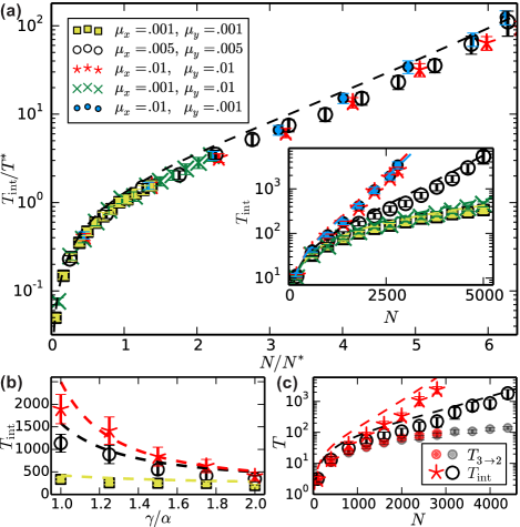
Figure 3: Mean time until transition from regular oscillations to intermittency. Dashed lines are from the analytical result (5). (a) Rescaled simulation data for $L=8$, $\alpha=\gamma=10$ and different choices of $\mu_{x/y}$ collapse onto a universal curve (unscaled data shown in the inset). (b) Transition times decrease for increasing $\gamma$ [parameters otherwise as in (a)]. (c) For $n=3$ virulent strains, the transition time $T_{3\to 2}$ until one strain is lost is much shorter than $T_{\text{int}}$, especially for large populations.

Conclusions.

We have analyzed a model for the coevolutionary dynamics of virus and immune system, combining simulations with nonlinear deterministic and stochastic analysis. Starting from the established quasispecies treatment of this problem, we explicitly introduced interactions between the populations. These lead to interdependent error thresholds, because a focused immune defense against a specific viral strain is impaired for large genetic variability in the virus population. Further, we performed a rigorous analysis of stochastic effects in the coexistence regime: regular yet noise-induced oscillatory behavior for large populations, large mutation rates, and weak immune response turn into stochastic intermittent cycles for smaller populations, smaller mutation rates and strong immune response. Our simulations indicate that the reverse transition from intermittency towards regular oscillations is a rare event occurring on time scales well beyond $T_{\text{int}}$. It cannot easily be analyzed within our reduced two-dimensional model as it will depend on the entire population structure. Finally, we note that our abstract model based on quasispecies theory focuses on the dynamics of genetic variability within populations of constant size. This assumption is of course violated for some biological scenarios, where immune response modulates the viral load Nowak1990 ; Wang2006 ; Bull2007 and may well lead to extinction of the virus Tejero2010 ; Woo2012 . We expect that more detailed models including these and other effects relevant in biological situations Bianconi2010 ; Alberts2002 will also be amenable to theoretical analysis based on the stochastic averaging techniques used here.

See pages ,1,,2,,3,,4,,5,,6,,7,,8,,9,,10,,11, of supplement_proof.pdf