Exit Probabilities for a Chain of Distributed Control Systems with Small Random Perturbations

Abstract

In this paper, we consider a diffusion process pertaining to a chain of distributed control systems with small random perturbation. The distributed control system is formed by $n$ subsystems that satisfy an appropriate Hörmander condition, i.e., the second subsystem assumes the random perturbation entered into the first subsystem, the third subsystem assumes the random perturbation entered into the first subsystem then was transmitted to the second subsystem and so on, such that the random perturbation propagates through the entire distributed control system. Note that the random perturbation enters only in one of the subsystems and, hence, the diffusion process is degenerate, in the sense that the backward operator associated with it is a degenerate parabolic equation. Our interest is to estimate the exit probability with which a diffusion process (corresponding to a particular subsystem) exits from a given bounded open domain during a certain time interval. The method for such an estimate basically relies on the interpretation of the exit probability function as a value function for a family of stochastic control problems that are associated with the underlying chain of distributed control systems.

I Introduction

In this paper, we consider the problem of estimating probabilities with which the diffusion process $x^{\epsilon,i}(t)$, for $i=1,2,\ldots,n$, exits from a given bounded open domain during a certain time interval pertaining to the following $n$ distributed control systems (see Fig. 1c)

$$\left.\begin{array}[]{l}dx^{\epsilon,1}(t)=f_{1}\bigl{(}t,x^{\epsilon,1}(t),u_{1}(t)\bigr{)}dt+\sqrt{\epsilon}\sigma\bigl{(}t,x^{\epsilon,1}(t))dW(t)\\ dx^{\epsilon,2}(t)=f_{2}\bigl{(}t,x^{\epsilon,1}(t),x^{\epsilon,2}(t),u_{2}(t)\bigr{)}dt\\ \quad\quad\quad~{}\vdots\\ dx^{\epsilon,i}(t)=f_{i}\bigl{(}t,x^{\epsilon,1}(t),x^{\epsilon,2}(t),\ldots,x^{\epsilon,i}(t),u_{i}(t)\bigr{)}dt\\ \quad\quad\quad~{}\vdots\\ dx^{\epsilon,n}(t)=f_{n}\bigl{(}t,x^{\epsilon,1}(t),x^{\epsilon,2}(t),\ldots,x^{\epsilon,n}(t),u_{n}(t)\bigr{)}dt\\ x^{\epsilon,1}(s)=x_{s}^{\epsilon,1},\,\,x^{\epsilon,2}(s)=x_{s}^{\epsilon,2},\,\,\ldots,\,\,x^{\epsilon,n}(s)=x_{s}^{\epsilon,n},\,\,s\leq t\leq T\end{array}\right\}$$ (8)

where

• $x^{\epsilon,i}(\cdot)$ is an $\mathbb{R}^{d}$-valued diffusion process that corresponds to the $i$th-subsystem,

• the functions $f_{i}\colon[0,\infty)\times\mathbb{R}^{i\times d}\times\mathcal{U}_{i}\rightarrow\mathbb{R}^{d}$ are uniformly Lipschitz, with bounded first derivatives, $\epsilon$ is a small positive number (which represents the level of random perturbation in the system),

• $\sigma\colon[0,\infty)\times\mathbb{R}^{d}\rightarrow\mathbb{R}^{d\times m}$ is Lipschitz with the least eigenvalue of $\sigma(\cdot,\cdot)\,\sigma^{T}(\cdot,\cdot)$ uniformly bounded away from zero, i.e.,

  $$\sigma(t,x)\,\sigma^{T}(t,x)\geq\lambda I_{d\times d},\quad\forall x\in\mathbb{R}^{d},$$

  for some $\lambda>0$,

• $W(\cdot)$ is a $d$-dimensional standard Wiener process (with $W(0)=0$),

• $u_{i}(\cdot)$ is a $\,\mathcal{U}_{i}$-valued measurable control process to the $i$th-subsystem (i.e., an admissible control from the measurable set $\mathcal{U}_{i}\subset\mathbb{R}^{r_{i}}$) such that for all $t>s$, $W(t)-W(s)$ is independent of $u_{i}(\nu)$ for $\nu\leq s$ (nonanticipativity condition) and

  $$\mathbb{E}\int_{s}^{t_{1}}|u_{i}(t)|^{2}dt<\infty,\quad\forall t_{1}\geq s,$$

for $i=1,2,\ldots,n$.

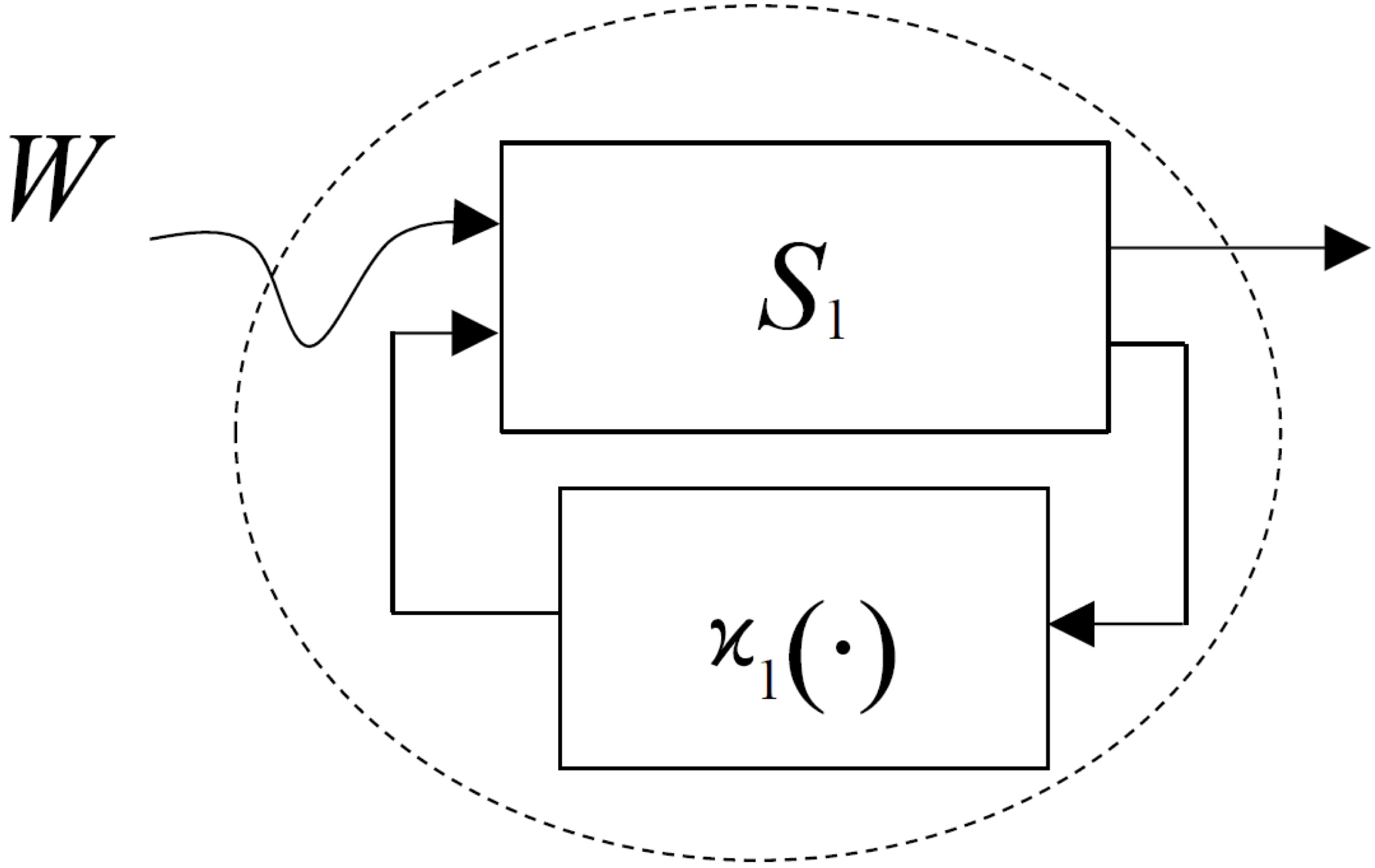
(a)

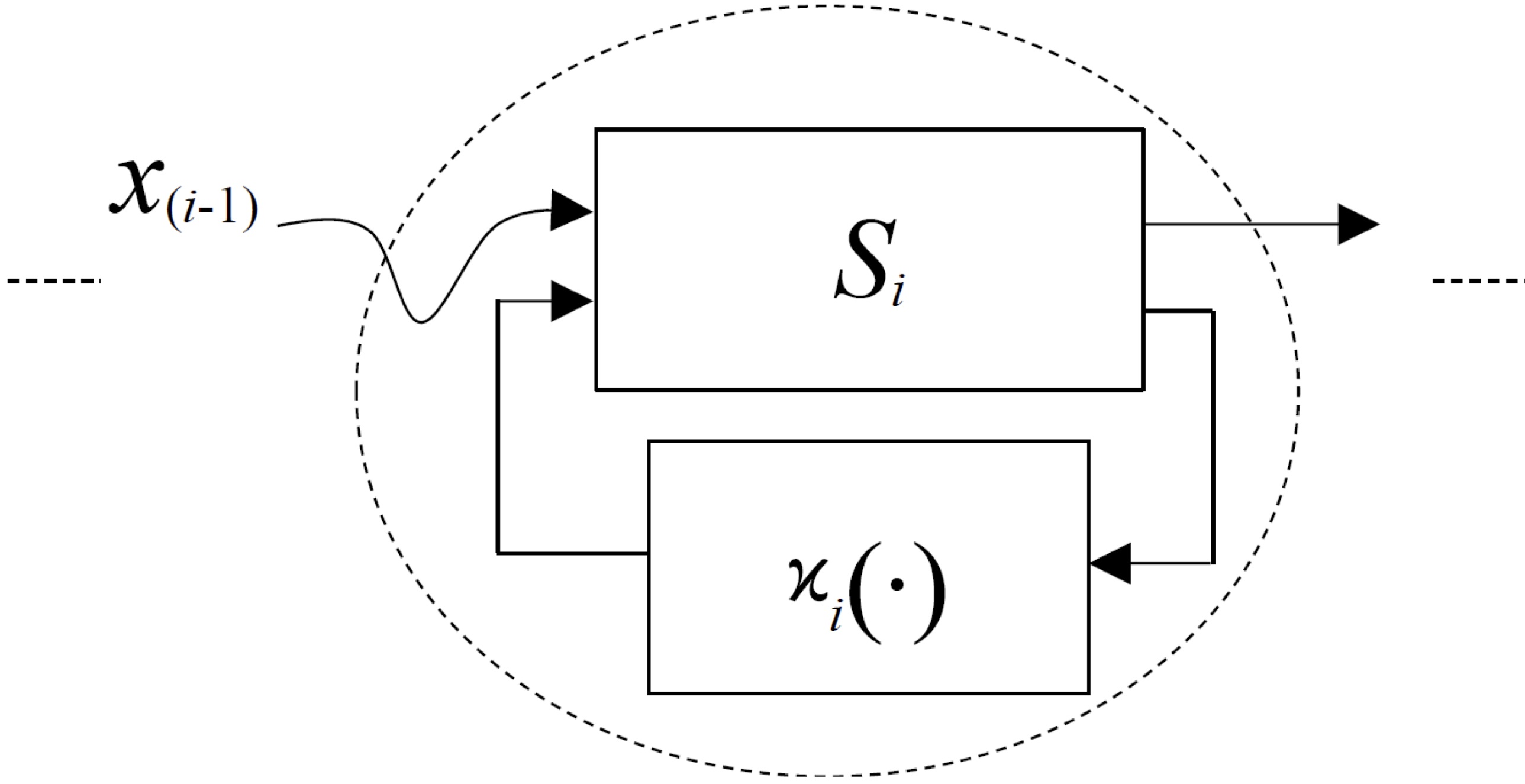
(b)

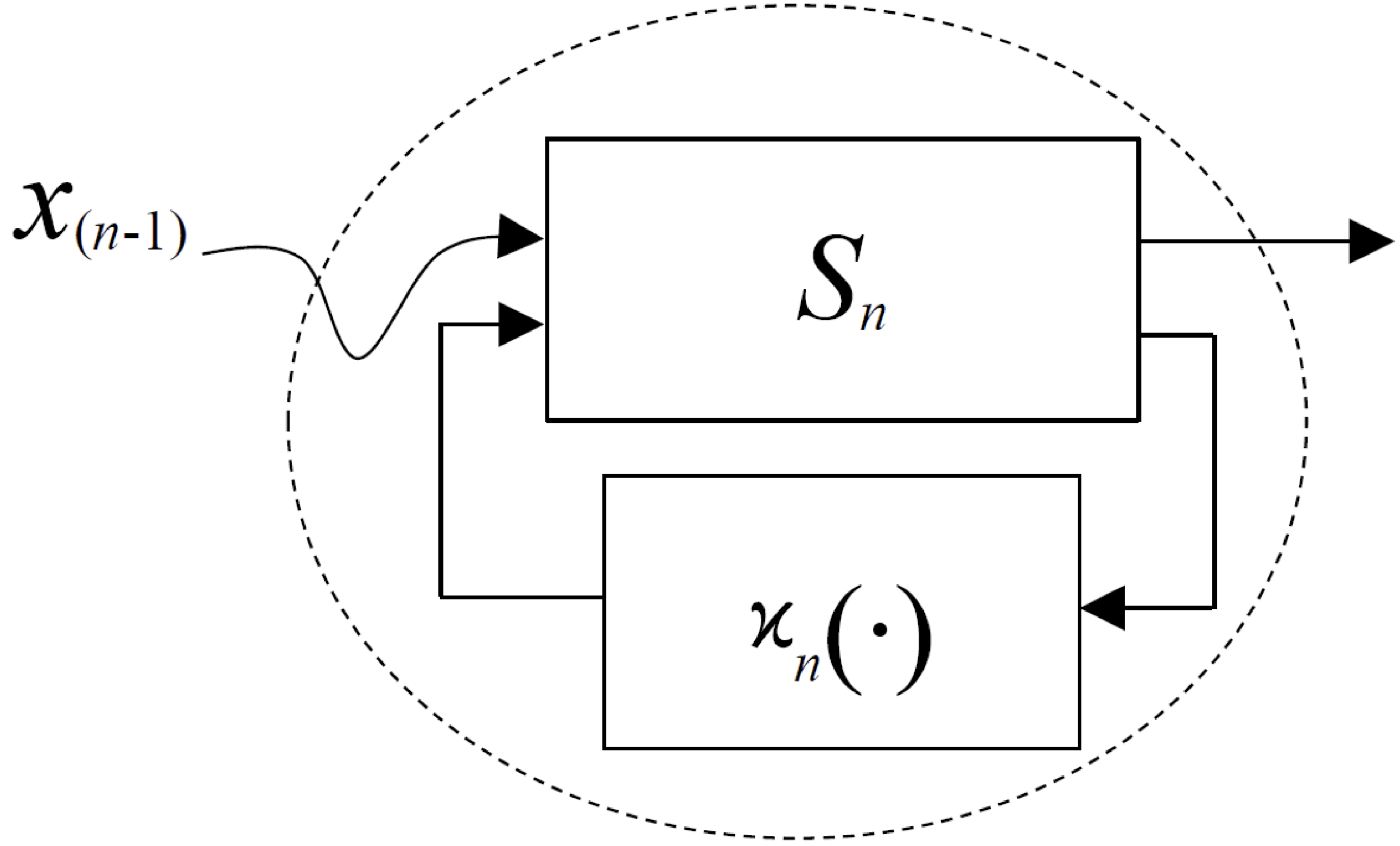
(c)

Figure 1: A chain of distributed control systems with small random perturbations

$\begin{array}[]{r@{\ }c@{\ }l}\vspace{-5 mm}{}\hfil\\ \text{where}&\\ &S_{1}:\,\,dx^{\epsilon,1}(t)=f_{1}\bigl{(}t,x^{\epsilon,1}(t),u_{1}(t)\bigr{)}dt+\sqrt{\epsilon}\sigma\bigl{(}t,x^{\epsilon,1}(t))dW(t),\\ &S_{i}:\,\,dx^{\epsilon,i}(t)=f_{i}\bigl{(}t,x^{\epsilon,1}(t),x^{\epsilon,2}(t),\ldots,x^{\epsilon,i}(t),u_{i}(t)\bigr{)}dt,~{}i=2,3,\ldots n,\\ &\quad\quad u_{j}(t)=\kappa_{j}(x^{\epsilon,j}(t)),~{}t\in[s,T],~{}j=1,2,\ldots n.\end{array}$

In what follows, we consider a particular class of admissible controls $u_{i}(\cdot)\in\mathcal{U}_{i}$, for $i=1,2\ldots,n$, of the form $\kappa_{i}(x^{\epsilon,i}(t))$, $\forall t\geq s$, with a measurable map $\kappa_{i}$ from $\mathbb{R}^{d}$ to $\mathcal{U}_{i}$ and, thus, such a measurable map $\kappa_{i}$ is called a stationary Markov control.

Remark 1

Note that, in Equation (8), the function $f_{i}$, with the admissible control $\kappa_{i}(x^{\epsilon,i})$, depends only on $x^{\epsilon,1}(t)$, $x^{\epsilon,2}(t)$, …, $x^{\epsilon,i}(t)$ and satisfies an appropriate Hörmander condition (e.g., see [11] for further discussion). Furthermore, the random perturbation has to pass through the second subsystem, the third subsystem, …, and the $(i-1)$th-subsystem to reach for the $i$th-subsystem. Hence, such a chain of distributed control systems is described by an $n\times d$-dimensional diffusion process, which is degenerate in the sense that the backward operator associated with it is a degenerate parabolic equation.

Let $D\subset\mathbb{R}^{d}$ be a bounded open domain with smooth boundary (i.e., $\partial D$ is a manifold of class $C^{2}$). Moreover, let $\tau_{D}^{\epsilon,\ell}=\tau_{D}^{\epsilon,{\ell}}(s,x^{\epsilon,1},\ldots,x^{\epsilon,\ell})$, for $\ell=2,3,\ldots,n$, be the first exit-time for the diffusion process $x^{\epsilon,\ell}(t)$ (corresponding to the $\ell$th-subsystem, with the admissible control $\kappa_{\ell}(\xi^{\ell}(t))$, for $t\geq s\geq 0$) from the given domain $D$, i.e.,

$$\tau_{D}^{\epsilon,\ell}=\inf\Bigl{\{}t>s\,\bigl{|}\,x^{\epsilon,\ell}(t)\in\partial D\Bigr{\}},$$ (9)

which depends on the behavior of the solutions to the following (deterministic) chain of distributed control systems, i.e.,

$$d\xi^{j}(t)=\hat{f}_{j}(t,\xi^{1}(t),\ldots,\xi^{j}(t)\bigr{)}dt,\quad\xi^{j}(s)=x_{s}^{j},\quad s\leq t\leq T,$$ (10)

for $j=1,\ldots,\ell$, with

$$\hat{f}_{j}(t,\xi^{1}(t),\ldots,\xi^{j}(t))\triangleq f_{j}(t,\xi^{1}(t),\ldots,\xi^{j}(t),\kappa_{j}(\xi^{j}(t))).$$

For a fixed (given) $T$, let us define the exit probability as

$$q^{\epsilon,\ell}\bigl{(}s,x^{\epsilon,1},\ldots,x^{\epsilon,\ell}\bigr{)}=\mathbb{P}_{s,x_{\widehat{1,\ell}}}^{\epsilon}\Bigl{\{}\tau_{D}^{\epsilon,\ell}\leq T\Bigr{\}},\quad\ell=2,3,\ldots,n,$$ (11)

where such a probability $\mathbb{P}_{s,x_{\widehat{1,\ell}}}^{\epsilon}\bigl{\{}\cdot\bigr{\}}$ is conditioned on the initial points $x_{s}^{\epsilon,j}\in\mathbb{R}^{d}$, for $j=1,\ldots\ell$, as well as on the class of admissible controls.

Notice that the backward operator for the diffusion process $\bigl{(}x^{\epsilon,1}(t),\ldots,x^{\epsilon,\ell}(t)\bigr{)}$, with $\kappa_{j}(x^{\epsilon,j}(t))$, for $j=1,\ldots,\ell$ and $\forall t\geq s$, when applied to a certain function $\upsilon^{\epsilon,\ell}\bigl{(}s,x^{\epsilon,1},\ldots,x^{\epsilon,\ell}\bigr{)}$, is given by

$$\upsilon_{s}^{\epsilon,\ell}+\mathcal{L}^{\epsilon,\ell}\upsilon^{\epsilon,\ell}\triangleq\upsilon_{s}^{\epsilon,\ell}+\frac{\epsilon}{2}\operatorname{tr}\Bigl{\{}a\,\upsilon_{x^{\epsilon,1}x^{\epsilon,1}}^{\epsilon,\ell}\Bigr{\}}+\sum\nolimits_{j=1}^{\ell}\hat{f}_{j}^{T}\upsilon_{x^{\epsilon,j}}^{\epsilon,\ell},$$ (12)

for $j=1,\ldots,\ell$, with $a(s,x^{\epsilon,1})=\sigma(s,x^{\epsilon,1})\,\sigma^{T}(s,x^{\epsilon,1})$ and

$$\hat{f}_{j}\bigl{(}t,x^{\epsilon,1}(t),\ldots,x^{\epsilon,j}(t))=f_{j}\bigl{(}t,x^{\epsilon,1}(t),\ldots,x^{\epsilon,j}(t),\kappa_{j}(x^{\epsilon,j}(t))).$$

Let $\Omega_{\ell}$ be the open set

$$\Omega_{\ell}=(0,T)\times\mathbb{R}^{(\ell-1)\times d}\times D,\quad\ell=2,3,\ldots,n.$$

Further, let us denote by $C^{\infty}(\Omega_{\ell})$ the spaces of infinitely differentiable functions on $\Omega_{\ell}$, and by $C_{0}^{\infty}(\Omega_{\ell})$ the space of the functions $\phi\in C^{\infty}(\Omega_{\ell})$ with compact support in $\Omega_{\ell}$. A locally square integrable function $\upsilon^{\epsilon,\ell}\bigl{(}s,x^{\epsilon,1},\ldots,x^{\epsilon,\ell}\bigr{)}$ on $\Omega_{\ell}$ is said to be a probabilistic solution to the following equation

$$\upsilon_{s}^{\epsilon,\ell}+\mathcal{L}^{\epsilon,\ell}\upsilon^{\epsilon,\ell}=0,$$ (13)

if, for any test function $\phi\in C_{0}^{\infty}(\Omega_{\ell})$, the following holds true

$$\int_{\Omega_{\ell}}\Bigl{(}-\phi_{t}+{\mathcal{L}^{\epsilon,\ell}}^{\ast}\phi\Bigr{)}\upsilon^{\epsilon,\ell}d\Omega_{\ell}=0,\quad\ell=2,3,\ldots,n,$$ (14)

where $d\Omega_{\ell}$ denotes the Lebesgue measure on $\mathbb{R}^{(\ell\times d)+1}$ and ${\mathcal{L}^{\epsilon,\ell}}^{\ast}$ is an adjoint operator corresponding to $\mathcal{L}^{\epsilon,\ell}$

$${\mathcal{L}^{\epsilon,\ell}}^{\ast}\phi=\frac{\epsilon}{2}\sum\nolimits_{j=1}^{d}\sum\nolimits_{m=1}^{d}\bigr{(}a_{j,m}\phi\bigr{)}_{x_{j}^{\epsilon,1}x_{m}^{\epsilon,1}}-\sum\nolimits_{j=1}^{\ell}\sum\nolimits_{m=1}^{d}\bigl{(}\hat{f}_{j}\phi\bigr{)}_{x_{m}^{\epsilon,j}}.$$ (15)

In this paper, we assume that the following statements hold for the chain of distributed control systems in Equation (8).

Assumption 1

1. The functions $f_{i}$, for $i=1,2,\ldots,n$, are bounded $C^{\infty}(\Omega_{0,i})$-functions, with bounded first derivatives, where $\Omega_{0,i}=(0,\infty)\times\mathbb{R}^{(i\times d)}$. Moreover, $\sigma$ and $\sigma^{-1}$ are bounded $C^{\infty}\bigl{(}(0,\infty)\times\mathbb{R}\bigr{)}$-functions, with bounded first derivatives.

2. The backward operator in Equation (12) is hypoelliptic in $C^{\infty}(\Omega_{0,\ell})$, for each $\ell=2,3,\ldots,n$ (e.g., see [11] or [4]).

3. For each $\ell=2,3,\ldots,n$, let $n(x^{\epsilon,\ell})$ be the outer normal vector to $\partial D$ and, further, let $\Gamma_{\ell}^{+}$ and $\Gamma_{\ell}^{0}$ denote the sets of points $(t,x^{\epsilon,1},\ldots,x^{\epsilon,\ell})$, with $x^{\epsilon,\ell}\in\partial D$, such that

   $$\hat{f}_{\ell}^{T}(t,x^{\epsilon,1},\ldots,x^{\epsilon,\ell})n(x^{\epsilon,\ell})$$

   is positive and zero, respectively.

Remark 2

Note that, from Assumptions 1(a)-(b), each matrix $\Bigr{(}\frac{\partial{f_{\ell}}_{i}}{\partial x_{j}^{\epsilon,1}}\Bigl{)}_{ij}$, for $\ell=2,3,\ldots n$, has full rank $d$ everywhere in $\Omega_{0,\ell}$, since the backward operator in Equation (12) is hypoelliptic. In particular, the hypoellipticity assumption is related to a strong accessibility property of controllable nonlinear systems that are driven by white noise (e.g., see [4, Section 3] for further discussion). That is, the hypoellipticity assumption implies that the diffusion process $x^{\epsilon,\ell}(t)$ has a transition probability density $p\bigl{(}t,(x^{\epsilon,1},\ldots,x^{\epsilon,\ell});\mu\bigr{)}$, which is $C^{\infty}$ on $(0,\infty)\times\mathbb{R}^{2(d\times\ell)}$, and which also satisfies the forward equation $p_{t}={\mathcal{L}^{\epsilon,\ell}}^{\ast}p$ (in the variables $(t,\mu))$.

In Section II, we present our main result – where, using the Ventcel-Freidlin asymptotic estimates [15] (cf. [9, Chapter 14] or [8]) and the stochastic control arguments from Fleming [7], we provide an asymptotic bound on the exit probability $q^{\epsilon,\ell}\bigl{(}s,x^{\epsilon,1},\ldots,x^{\epsilon,\ell}\bigr{)}$, i.e.,

$$I^{\epsilon,\ell}\bigl{(}s,x^{\epsilon,1},\ldots,x^{\epsilon,\ell}\bigr{)}\rightarrow I^{0,\ell}\bigl{(}s,x^{\epsilon,1},\ldots,x^{\epsilon,\ell}\bigr{)}\quad\text{as}\quad\epsilon\rightarrow 0,$$

where

$$I^{\epsilon,\ell}\bigl{(}s,x^{\epsilon,1},\ldots,x^{\epsilon,\ell}\bigr{)}=-\epsilon\log q^{\epsilon,\ell}\bigl{(}s,x^{\epsilon,1},\ldots,x^{\epsilon,\ell}\bigr{)},\quad\ell=2,3,\ldots,n.$$

Such an asymptotic estimate for $I^{\epsilon,\ell}\bigl{(}s,x^{\epsilon,1},\ldots,x^{\epsilon,\ell}\bigr{)}$ relies on the interpretation of the exit probability function as a value function for a family of stochastic control problems that can be associated with the underlying chain of distributed control systems. Finally, we provide concluding remarks in Section III.

Before concluding this section, it is worth mentioning that some interesting studies on the asymptotic behavior of exit probabilities for dynamical systems with small random perturbations have been reported in literature (for example, see [10], [3] or [14] in the context of estimating density functions for degenerate diffusions; see [13] or [2] in the context of nondegenerate diffusions; and see also [1] in the context of exit-time and invariant measure for small noise constrained diffusions).

II Main Results

II-A The exit probabilities

Let $(x^{\epsilon,1}(t),x^{\epsilon,2}(t),\ldots,x^{\epsilon,\ell}(t))$, with $\ell=2,3,\ldots,n$, for $0\leq t\leq T$, be the diffusion process. Further, let us consider the following boundary value problem

$$\left.\begin{array}[]{c}\upsilon_{s}^{\epsilon,\ell}+\mathcal{L}^{\epsilon,\ell}\upsilon^{\epsilon,\ell}=0\quad\text{in}\quad\Omega_{\ell}=(0,T)\times\mathbb{R}^{(\ell-1)\times d}\times D\\ \upsilon^{\epsilon,\ell}\bigl{(}s,x^{\epsilon,1},\ldots,x^{\epsilon,\ell}\bigr{)}=1\quad\text{on}\quad\Gamma_{T,\ell}^{+}\\ \upsilon^{\epsilon,\ell}\bigl{(}s,x^{\epsilon,1},\ldots,x^{\epsilon,\ell}\bigr{)}=0\quad\text{on}\quad\{T\}\times\mathbb{R}^{(\ell-1)\times d}\times D\end{array}\right\}$$ (19)

where $\mathcal{L}^{\epsilon,\ell}$ is the backward operator in Equation (12) and

$$\Gamma_{T,\ell}^{+}=\Bigl{\{}\bigl{(}s,x^{\epsilon,1},\ldots,x^{\epsilon,\ell}\bigr{)}\in\Gamma_{\ell}^{+}\,\bigl{|}\,0<s\leq T\Bigr{\}}.$$

Let $\Omega_{0T,\ell}$ be the set consisting of $\Omega_{\ell}\bigcup\{T\}\times\mathbb{R}^{(\ell-1)\times d}\times D$, together with the boundary points $\bigl{(}s,x^{\epsilon,1},\ldots,x^{\epsilon,\ell}\bigr{)}\in\Gamma_{\ell}^{+}$, with $0<s<T$. Then, the following proposition provides a solution to the exit probability $\mathbb{P}_{s,x_{\widehat{1,\ell}}}^{\epsilon}\Bigl{\{}\tau_{D}^{\epsilon,\ell}\leq T\Bigr{\}}$, for each $\ell=2,3,\ldots,n$, with which the diffusion process $x^{\epsilon,\ell}(t)$ exits from the domain $D$.

Proposition 1

Suppose that the statements (a)-(c) in the above assumption (i.e., Assumption 1) hold true. Then, the exit probability $q^{\epsilon,\ell}(s,x^{\epsilon,1},\ldots,x^{\epsilon,\ell})=\mathbb{P}_{s,x_{\widehat{1,\ell}}}^{\epsilon}\bigl{\{}\tau_{D}^{\epsilon,\ell}\leq T\bigr{\}}$ is a smooth solution to the boundary value problem in Equation (19), and, moreover, it is a continuous function on $\Omega_{0T,\ell}$.

In order to prove the above proposition, we consider the following nondegenerate diffusion process $(x^{\epsilon,1}(t),x^{\delta_{2},\epsilon,2}(t),\ldots,x^{\delta_{\ell},\epsilon,\ell}(t))$ satisfying

$$\left.\begin{array}[]{l}dx^{\epsilon,1}(t)=\hat{f}_{1}\bigl{(}t,x^{\epsilon,1}(t)\bigr{)}dt+\sqrt{\epsilon}\sigma\bigl{(}t,x^{\epsilon,1}(t))dW(t)\\ dx^{\delta_{\ell},\epsilon,\ell}(t)=\hat{f}_{\ell}\bigl{(}t,x^{\epsilon,1}(t),x^{\delta_{2},\epsilon,2}(t),\ldots,x^{\delta_{\ell},\epsilon,\ell}(t)\bigr{)}dt+\sqrt{\delta_{\ell}}dW_{\ell}(t)dt,\\ \quad\quad\quad\quad\quad\quad\quad\quad\quad\quad\quad\quad\quad\quad\quad\delta_{\ell}>0,\,\,s\leq t\leq T\end{array}\right\}$$ (23)

for $\ell=2,3,\ldots,n$, with an initial condition

$$\bigl{(}x^{\epsilon,1}(s),x^{\delta_{2},\epsilon,2}(s),\ldots,x^{\delta_{\ell},\epsilon,\ell}(s)\bigr{)}=\bigl{(}x_{s}^{\epsilon,1},x_{s}^{\epsilon,2},\ldots,x_{s}^{\epsilon,\ell}\bigr{)}.$$ (24)

Moreover, $W_{j}(\cdot)$, for $j=2,\ldots,\ell$, are $d$-dimensional standard Wiener processes (with $W_{\ell}(0)=0$) and independent to $W(\cdot)$.

Let $\tau_{D}^{\delta,\epsilon,\ell}=\tau_{D}^{\delta,\epsilon,{\ell}}(s,x^{\epsilon,1},x^{\delta_{2},\epsilon,2},\ldots,x^{\delta_{\ell},\epsilon,\ell})$ be the first exit-time for the diffusion process $x^{\delta_{\ell},\epsilon,\ell}(t)$ (corresponding to the $\ell$th-subsystem, with a nondegenerate case) from the domain $D$. Later, we relate the exit probability of this diffusion process with that of the boundary value problem in Equation (19) as the limiting case, when $\delta_{\ell}\rightarrow 0$, for $\ell=2,3,\dots,n$.

Next, let us define the following

$$\begin{array}[]{c}\theta=\tau_{D}^{\epsilon,\ell}\wedge T,\quad\quad\theta^{\delta}=\tau_{D}^{\delta,\epsilon,\ell}\wedge T,\\ \bigl{\|}x^{\delta_{\ell},\epsilon,\ell}-x^{\epsilon,\ell}\bigr{\|}_{t}=\sup\limits_{s\leq r\leq t}\Bigl{|}x^{\delta_{\ell},\epsilon,\ell}(r)-x^{\epsilon,\ell}(r)\Bigr{|},\quad\ell=2,3,\ldots,n.\end{array}$$

Then, we need the following lemma, which is useful for proving the above proposition.

Lemma 1

Suppose that $\epsilon>0$ is fixed. Then, for any initial point $(x^{\epsilon,1},\ldots,x^{\epsilon,\ell})\in\mathbb{R}^{(\ell-1)\times d}\times D$, with $t>s$, the following statements hold true

1. $\bigl{\|}x^{\delta_{\ell},\epsilon,\ell}-x^{\epsilon,\ell}\bigr{\|}_{t}\rightarrow 0$,

2. $\theta^{\delta}\rightarrow\theta$, and

3. $\bigl{(}x^{\delta_{2},\epsilon,2}(\theta^{\delta}),\ldots,x^{\delta_{\ell},\epsilon,\ell}(\theta^{\delta})\bigr{)}\rightarrow\bigl{(}x^{\epsilon,2}(\theta),\ldots,x^{\epsilon,\ell}(\theta)\bigr{)}$,

almost surely, as $\delta_{\ell}\rightarrow 0$, for $\ell=2,3,\ldots,n$.

Proof:

Part (i): Note that, for a fixed $\epsilon>0$ and $\ell\in\{2,3,\ldots,n\}$, the following inequality holds

$$\bigl{|}x^{\delta_{\ell},\epsilon,\ell}(r)-x^{\epsilon,\ell}(r)\bigr{|} \leq\int_{s}^{t}\Bigl{|}\hat{f}_{\ell}\bigl{(}r,x^{\epsilon,1}(r),\ldots,x^{\delta_{\ell},\epsilon,\ell}(r)\bigr{)}-\hat{f}_{\ell}\bigl{(}r,x^{\epsilon,1}(r),\ldots,x^{,\epsilon,\ell}(r)\bigr{)}\Bigr{|}dr$$

$$\quad\quad\quad\quad\quad\quad+\sqrt{\delta_{\ell}}|W_{\ell}(t)|,$$

$$\leq C\int_{s}^{t}\bigl{|}x^{\delta_{\ell},\epsilon,\ell}(r)-x^{\epsilon,\ell}(r)\bigr{|}+\sqrt{\delta_{\ell}}|W_{\ell}(t)|,$$

such that

$$\bigl{\|}x^{\delta_{\ell},\epsilon,\ell}(r)-x^{\epsilon,\ell}(r)\bigr{\|}_{t}\leq C\int_{s}^{t}\bigl{|}x^{\delta_{\ell},\epsilon,\ell}(r)-x^{\epsilon,\ell}(r)\bigr{|}+\sqrt{\delta_{\ell}}|W_{\ell}(t)|,$$

where $C$ is a Lipschitz constant. Using the Gronwall-Bellman inequality, we obtain the following

$$\bigl{\|}x^{\delta_{\ell},\epsilon,\ell}(r)-x^{\epsilon,\ell}(r)\bigr{\|}_{t}\leq c\sqrt{\delta_{\ell}}\bigl{\|}W_{\ell}\bigr{\|}_{t},$$

where $c$ is a constant that depends on $C$ and $(t-s)$. Hence, we have

$$\bigl{\|}x^{\delta_{\ell},\epsilon,\ell}(r)-x^{\epsilon,\ell}(r)\bigr{\|}_{t}\rightarrow 0\quad\text{as}\quad\delta_{\ell}\rightarrow 0,$$

for each $\ell=2,3,\ldots,n$.

Part (ii): Next, let us show $\theta$ satisfies the following bounds

$$\theta^{\ast}\leq\theta\leq\theta_{\ast},$$

almost surely, where $\theta^{\ast}=\limsup_{\delta_{\ell}\rightarrow 0}\theta^{\delta}$ and $\theta_{\ast}=\liminf_{\delta_{\ell}\rightarrow 0}\theta^{\delta}$, for $\ell=2,3,\ldots,n$.

Notice that $D$ is open, then it follows from Part (i) that if $\theta=\tau_{D}^{\epsilon,\ell}\wedge T=T$, then $\theta^{\delta}=T$, almost surely, for all $\delta_{\ell}$ sufficiently small. Then, we will get Part (ii). Similarly, if $\theta^{\delta}=T$ and $x^{\delta,\epsilon,\ell}(\theta^{\delta})\in D$, then the statement in Part (i) implies Part (ii). Then, we can assume that $x^{\epsilon,\ell}(\theta)\in\partial D$ and $x^{\delta,\epsilon,\ell}(\theta^{\delta})\in\partial D$. Moreover, if $x^{\delta,\epsilon,\ell}(\theta^{\delta})\in\partial D$, then, from Part (i), $x^{\epsilon,\ell}(\theta_{\ast})\in\partial D$, almost surely, and, consequently, $\theta_{\ast}\geq\theta$, almost surely.

For the case $\theta^{\ast}\leq\theta$, let us define an event $\Psi_{a,\alpha}$ (with $a>0$ and $\alpha>0$) as follow: there exists $t\in[\theta,\theta+a]$ such that the distance $\varrho\bigl{(}x^{\epsilon,\ell}(t),D\cup\partial D\bigr{)}\geq\alpha$. Notice that if this holds together with $\bigl{\|}x^{\delta_{\ell},\epsilon,\ell}-x^{\epsilon,\ell}\bigr{\|}_{t}<\alpha$, then we have $\theta^{\delta}<\theta+a$. Hence, from Part (i), we have $\theta^{\ast}<\theta+a$ on $\Psi_{a,\alpha}$, almost surely.

On the other hand, from Assumption 1(c), we have the following

$$\mathbb{P}_{s,x_{\widehat{1,\ell}}}^{\epsilon}\Bigl{\{}\bigcup\nolimits_{\alpha>0}\Psi_{a,\alpha}\Bigr{\}}=1.$$

Then,

$$\mathbb{P}_{s,x_{\widehat{1,\ell}}}^{\epsilon}\Bigl{\{}\theta^{\ast}<\theta+a\Bigr{\}}=1,$$

since $a$ is an arbitrary, we obtain $\theta^{\ast}<\theta$, almost surely.

Finally, notice that the statement in Part (iii) is a consequence of Part (i) and Part (ii). This completes the proof of Lemma 1. $\Box$

Proof:

Note that, from Assumption 1(c), it is sufficient to show that $q^{\epsilon,\ell}(s,x^{\epsilon,1},\ldots,x^{\epsilon,\ell})$ is a smooth solution (almost everywhere in $\Omega_{\ell}$ with respect to Lebesgue measure) to the boundary value problem in Equation (19).

For a fixed $\ell\in\{2,3,\ldots,n\}$, consider the following backward operator which corresponds to the nondegenerate diffusion process $(x^{\epsilon,1}(t),x^{\delta_{2},\epsilon,2}(t),\ldots,x^{\delta_{\ell},\epsilon,\ell}(t))$

$$\upsilon_{s}^{\delta,\epsilon,\ell}+\mathcal{L}^{\epsilon,\ell}\upsilon^{\delta,\epsilon,\ell}+\sum\nolimits_{j=2}^{\ell}\frac{\delta_{j}}{2}\triangle_{x^{\delta_{j},\epsilon,j}}\upsilon^{\delta,\epsilon,\ell}=0\quad\text{in}\quad\Omega_{\ell}=(0,T)\times\mathbb{R}^{(\ell-1)\times d}\times D,$$ (25)

where $\triangle_{x^{\delta_{j},\epsilon,j}}$ is the Laplace operator in the variable $x^{\delta_{j},\epsilon,j}$ and $\mathcal{L}^{\epsilon,\ell}$ is the backward operator in Equation (12).

Next, define $\partial^{\ast}D$ as $\{T\}\times\mathbb{R}^{(\ell-1)\times d}\times D$, together with the boundary points $\bigl{(}s,x^{\epsilon,1},x^{\delta_{2},\epsilon,2},\\ \ldots,x^{\delta_{\ell},\epsilon,\ell}\bigr{)}\in\Gamma_{\ell}^{+}$, with $0<s<T$. Let $\psi\bigl{(}s,x^{\epsilon,1},x^{\delta_{2},\epsilon,2},\ldots,x^{\delta_{\ell},\epsilon,\ell}\bigr{)}$ be a function which is continuous on $\partial D$. Note that, from Assumption 1(c), the backward operator in Equation (25) is uniformly parabolic and, therefore, its solution satisfies the following boundary condition

$$\upsilon^{\delta,\epsilon,\ell}\bigl{(}s,x^{\epsilon,1},x^{\delta_{2},\epsilon,2},\ldots,x^{\delta_{\ell},\epsilon,\ell}\bigr{)}=\psi\bigl{(}s,x^{\epsilon,1},x^{\delta_{2},\epsilon,2},\ldots,x^{\delta_{\ell},\epsilon,\ell}\bigr{)}\quad\text{on}\quad\partial^{\ast}D,$$ (26)

where

$$\upsilon^{\delta,\epsilon,\ell}\bigl{(}s,x^{\epsilon,1},x^{\delta_{2},\epsilon,2},\ldots,x^{\delta_{\ell},\epsilon,\ell}\bigr{)}=\mathbb{E}_{s,x_{\widehat{1,\ell}}}^{\delta,\epsilon}\Bigl{\{}\psi\bigl{(}\theta^{\delta},x^{\epsilon,1},x^{\delta_{2},\epsilon,2},\ldots,x^{\delta_{\ell},\epsilon,\ell}\bigr{)}\Bigr{\}},$$ (27)

with $\theta^{\delta}=\tau_{D}^{\delta,\epsilon,\ell}\wedge T$.

In particular, let $\psi_{k}$, with $k=1,2,\ldots$, be a sequence of bounded functions that are continuous on $\partial^{\ast}D$ and satisfying the following conditions

$$\psi_{k}\bigl{(}s,x^{\epsilon,1},x^{\delta_{2},\epsilon,2},\ldots,x^{\delta,\epsilon,\ell}\bigr{)}=\left\{\begin{array}[]{l l}1&\text{if}\,\bigl{(}s,x^{\epsilon,1},x^{\delta_{2},\epsilon,2},\ldots,x^{\delta_{\ell},\epsilon,\ell}\bigr{)}\in\Gamma_{T,\ell}^{+}\\ 0&\text{if}\,\bigl{(}s,x^{\epsilon,1},x^{\delta_{2},\epsilon,2},\ldots,x^{\delta_{\ell},\epsilon,\ell}\bigr{)}\in\{T\}\times\mathbb{R}^{(\ell-1)\times d}\\ &\quad\quad\quad\quad\quad\quad\quad\quad\times D\quad\text{and}\quad\varrho\bigl{(}x^{\delta,\epsilon,\ell},\partial D\bigr{)}>\frac{1}{k}\end{array}\right.$$

and

$$0\leq\psi_{k}\bigl{(}s,x^{\epsilon,1},x^{\delta_{2},\epsilon,2},\ldots,x^{\delta_{\ell},\epsilon,\ell}\bigr{)}\leq 1\,\, \text{if}\,\,\bigl{(}s,x^{\epsilon,1},x^{\delta_{2},\epsilon,2},\ldots,x^{\delta,\epsilon,\ell}\bigr{)}\in\{T\}\times\mathbb{R}^{(\ell-1)\times d}$$

$$\quad\quad\quad\quad\quad\quad\times D\quad\text{and}\quad\varrho\bigl{(}x^{\delta,\epsilon,\ell},\partial D\bigr{)}\leq\tfrac{1}{k}.$$

Moreover, such bounded functions further satisfy the following

$$\bigl{|}\psi_{k}-\psi_{l}\bigr{|}\rightarrow 0\quad\text{as}\quad k,l\rightarrow\infty$$ (28)

uniformly on any compact subset of $\bar{\Omega}_{\ell}$. Then, with $\psi=\psi_{k}$,

$$\upsilon_{k}^{\delta,\epsilon,\ell}\bigl{(}s,x^{\epsilon,1},x^{\delta_{2},\epsilon,2},\ldots,x^{\delta,\epsilon,\ell}\bigr{)}=\mathbb{E}_{s,x_{\widehat{1,\ell}}}^{\delta,\epsilon}\Bigl{\{}\psi_{k}\bigl{(}\theta^{\delta},x^{\epsilon,1},x^{\delta_{2},\epsilon,2},\ldots,x^{\delta,\epsilon,\ell}\bigr{)}\Bigr{\}}$$

satisfies Equation (26) and Equation (27). Then, from the continuity of $\psi_{k}$ (cf. Lemma 1, Parts (i)-(iii)) and the Lebesgue’s dominated convergence theorem (see [12, Chapter 4]), we have the following

$$\upsilon_{k}^{\delta,\epsilon,\ell}\bigl{(}s,x^{\epsilon,1},x^{\delta_{2},\epsilon,2},\ldots,x^{\delta,\epsilon,\ell}\bigr{)}\rightarrow\underbrace{\mathbb{E}_{s,x_{\widehat{1,\ell}}}^{\delta,\epsilon}\Bigl{\{}\psi_{k}\bigl{(}\theta^{\delta},x^{\epsilon,1},x^{\delta_{2},\epsilon,2},\ldots,x^{\delta,\epsilon,\ell}\bigr{)}\Bigr{\}}}_{\triangleq q_{k}^{\epsilon,\ell}\bigl{(}s,x^{\epsilon,1},\ldots,x^{\epsilon,\ell}\bigr{)}}$$ (29)

as $\delta_{\ell}\rightarrow 0$, for $\ell=2,3,\ldots,n$, with $\theta=\tau_{D}^{\epsilon,\ell}\wedge T$. Furthermore, in the above equation, $\bigl{(}x^{\epsilon,1}(t),\ldots,x^{\epsilon,\ell}(t)\bigr{)}$ is a solution to Equation (23), when $\delta_{\ell}=0$, for $\ell=2,3,\ldots,n$, with an initial condition of Equation (24).

Notice that $q_{k}^{\epsilon,\ell}\bigl{(}s,x^{\epsilon,1},\ldots,x^{\epsilon,\ell}\bigr{)}$ satisfies the backward operator in Equation (25), with $\upsilon^{\delta,\epsilon,\ell}=\upsilon_{k}^{\delta,\epsilon,\ell}$, and, in addition, it is a distribution solution to the boundary value problem in Equation (19), i.e.,

$$\int_{\Omega_{\ell}}\Bigl{(}-\phi_{t}+{\mathcal{L}^{\epsilon,\ell}}^{\ast}\phi\Bigr{)}q_{k}^{\epsilon,\ell}d\Omega_{\ell}, =\lim_{\delta_{j}\rightarrow 0,\,\forall j\in\{2,\ldots,\ell\}}\int_{\Omega_{\ell}}\Bigl{(}-\phi_{t}+{\mathcal{L}^{\epsilon,\ell}}^{\ast}\phi$$

$$\quad\quad\quad\quad\quad\quad\quad+\sum\nolimits_{j=2}^{\ell}\frac{\delta_{j}}{2}\triangle_{x^{\delta_{j},\epsilon,j}}\phi\Bigr{)}\upsilon_{k}^{\delta,\epsilon,\ell}d\Omega_{\ell},$$

$$=0,$$

for any test function $\phi\in C_{0}^{\infty}(\Omega_{\ell})$.

Finally, notice that

$$q^{\epsilon,\ell}\bigl{(}s,x^{\epsilon,1},\ldots,x^{\epsilon,\ell}\bigr{)}=\lim_{k\rightarrow\infty}q_{k}^{\epsilon,\ell}\bigl{(}s,x^{\epsilon,1},\ldots,x^{\epsilon,\ell}\bigr{)},$$

almost everywhere in $\Omega_{\ell}$. From Assumption 1(b) (i.e., the hypoellipticity), $q^{\epsilon,\ell}\bigl{(}s,x^{\epsilon,1},\ldots,\\ x^{\epsilon,\ell}\bigr{)}$ is a smooth solution to Equation (19) (almost everywhere) in $\Omega_{\ell}$ and continuous on the boundary of $\Omega_{0T,\ell}$. This completes the proof of Proposition 1. $\Box$

Remark 3

Here, we remark that the statements in Proposition 1 will make sense only if we require the following

$$\tau_{D}^{\epsilon,1}\,\geq\,\tau_{D}^{\epsilon,2}\,\geq\,\cdots\,\geq\,\tau_{D}^{\epsilon,\ell},$$

where $\tau_{D}^{\epsilon,1}=\inf\bigl{\{}t>s\,\bigl{|}\,x^{\epsilon,1}(t)\in\partial D\bigr{\}}$. It should be noted that such a condition, in general, depends on the constituting subsystems in Equation (8), the admissible controls from the measurable sets $\prod_{j=1}^{\ell}\mathcal{U}_{j}$ and the given bounded open domain $D$.

II-B Connection with control problems

II-B1 Deterministic minimum control problems

Note that, from Proposition 1, the exit probability $q^{\epsilon,\ell}\bigl{(}s,x^{\epsilon,1},\ldots,x^{\epsilon,\ell}\bigr{)}$ is a smooth solution to the boundary value problem in Equation (19). Further, if we introduce the following logarithmic transformation (e.g., see [7] or [5])

$$I^{\epsilon,\ell}\bigl{(}s,x^{\epsilon,1},\ldots,x^{\epsilon,\ell}\bigr{)}=-\epsilon\log q^{\epsilon,\ell}\bigl{(}s,x^{\epsilon,1},\ldots,x^{\epsilon,\ell}\bigr{)}.$$ (30)

Then, the function $I^{\epsilon,\ell}\bigl{(}s,x^{\epsilon,1},\ldots,x^{\epsilon,\ell}\bigr{)}$ satisfies the following boundary value problem

$$\left.\begin{array}[]{c}I_{s}^{\epsilon,\ell}+\mathcal{L}^{\epsilon,\ell}I^{\epsilon,\ell}-\frac{1}{2}\bigl{(}I_{x^{\epsilon,1}}^{\epsilon,\ell}\bigr{)}^{T}a(s,x^{\epsilon,1})I_{x^{\epsilon,1}}^{\epsilon,\ell}=0\quad\text{in}\quad\Omega_{\ell}=(0,T)\times\mathbb{R}^{(\ell-1)\times d}\times D\\ I^{\epsilon,\ell}\bigl{(}s,x^{\epsilon,1},\ldots,x^{\epsilon,\ell}\bigr{)}=0\quad\text{on}\quad\Gamma_{T,\ell}^{+}\\ I^{\epsilon,\ell}\bigl{(}s,x^{\epsilon,1},\ldots,x^{\epsilon,\ell}\bigr{)}=\infty\quad\text{on}\quad\{T\}\times\mathbb{R}^{(\ell-1)\times d}\times D\end{array}\right\}$$ (34)

where $\mathcal{L}^{\epsilon,\ell}$ is backward operator in Equation (12). Observe that $I^{\epsilon,\ell}\bigl{(}s,x^{\epsilon,1},\ldots,x^{\epsilon,\ell}\bigr{)}$ further satisfies the following dynamic programming equation

$$0=I_{s}^{\epsilon,\ell}+\frac{\epsilon}{2}\operatorname{tr}\Bigl{\{}a\,I_{x^{\epsilon,1}x^{\epsilon,1}}^{\epsilon,\ell}\Bigr{\}}+\sum\nolimits_{j=1}^{\ell}\hat{f}_{j}^{T}\bigl{(}s,x^{\epsilon,1},\ldots,x^{\epsilon,j}\bigr{)}I_{x^{\epsilon,j}}^{\epsilon,\ell}$$

$$\quad\quad\quad+H^{\epsilon,\ell}\bigl{(}s,x^{\epsilon,1},I_{x^{\epsilon,1}}^{\epsilon,\ell}\bigr{)}\quad\text{in}\quad\Omega_{\ell},$$ (35)

for $\ell=2,3,\ldots,n$, where

$$H^{\epsilon,\ell}\bigl{(}s,x^{\epsilon,1},p\bigr{)}=\hat{f}_{1}^{T}(s,x^{\epsilon,1})p-\frac{1}{2}p^{T}\Bigl{[}a(s,x^{\epsilon,1})\Bigr{]}^{-1}p.$$ (36)

Next, we define $L^{\epsilon,\ell}\bigl{(}s,x^{\epsilon,1},\hat{u}\bigr{)}$ as

$$L^{\epsilon,\ell}\bigl{(}s,x^{\epsilon,1},\hat{u}\bigr{)}=\frac{1}{2}\Bigl{(}\hat{f}_{1}(s,x^{\epsilon,1})-\hat{u}\Bigr{)}^{T}\Bigl{[}a(s,x^{\epsilon,1})\Bigr{]}^{-1}\Bigl{(}\hat{f}_{1}(s,x^{\epsilon,1})-\hat{u}\Bigr{)}.$$ (37)

Then, we observe that there is a duality between $H^{\epsilon,\ell}\bigl{(}s,x^{\epsilon,1},p\bigr{)}$ and $L^{\epsilon,\ell}\bigl{(}s,x^{\epsilon,1},\hat{u}\bigr{)}$ such that

$$L^{\epsilon,\ell}\bigl{(}s,x^{\epsilon,1},\hat{u}\bigr{)}=\sup_{p}\biggl{\{}H^{\epsilon,\ell}\bigl{(}s,x^{\epsilon,1},p\bigr{)}-p^{T}\hat{u}\biggr{\}}$$ (38)

and

$$H^{\epsilon,\ell}\bigl{(}s,x^{\epsilon,1},p\bigr{)}=\inf_{\hat{u}}\biggl{\{}L\bigl{(}s,x^{\epsilon,1},\hat{u}\bigr{)}+p^{T}\hat{u}\biggr{\}}.$$ (39)

Furthermore, if we set $\epsilon=0$ in Equation (35), then we have the following dynamic programming equation (e.g., see [6, Chapter 4])

$$I_{s}^{0,\ell}+\sum\nolimits_{j=1}^{\ell}\hat{f}_{j}^{T}\bigl{(}s,x^{\epsilon,1},\ldots,x^{\epsilon,j}\bigr{)}I_{x^{\epsilon,j}}^{0,\ell}+\inf_{\hat{u}}\biggl{\{}L^{\epsilon,\ell}\bigl{(}s,x^{\epsilon,1},\hat{u}\bigr{)}+\bigl{(}I_{x^{\epsilon,1}}^{0,\ell}\bigr{)}^{T}\hat{u}\biggr{\}}=0,$$ (40)

for a family of deterministic minimum control problems corresponding to the following system of equations

$$\left.\begin{array}[]{l}dx^{0,1}(t)=\hat{u}(t)dt\\ dx^{0,\ell}(t)=\hat{f}_{\ell}\bigl{(}t,x^{0,1}(t),\ldots,x^{0,\ell}(t)\bigr{)}dt,\quad s\leq t\leq T\end{array}\right\}$$ (43)

for $\ell=2,3,\ldots,n$, with an initial condition

$$\bigl{(}x^{0,1}(s),\ldots,x^{0,\ell}(s)\bigr{)}=\bigl{(}x_{s}^{\epsilon,1},\ldots,x_{s}^{\epsilon,\ell}\bigr{)}$$

and the associated value functions

$$I^{0,\ell}\bigl{(}s,x^{\epsilon,1},\ldots,x^{\epsilon,\ell}\bigr{)}=\inf_{\hat{u}\in\hat{U}\bigl{(}s,x_{s}^{\epsilon,1},\ldots,x_{s}^{\epsilon,\ell}\bigr{)}}\int_{s}^{\theta}L^{\epsilon,\ell}\bigl{(}t,x^{0,1}(t),\hat{u}(t)\bigr{)}dt,$$ (44)

where $\theta$ is the exit-time for $x^{0,\ell}(t)$ from the domain $D$, $\hat{U}\bigl{(}s,x^{\epsilon,1},\ldots,x^{\epsilon,\ell}\bigr{)}$ is a class of continuous functions for which $\theta\leq T$, and $\bigl{(}\theta,x^{0,1}(\theta),\ldots,x^{0,\ell}(\theta)\bigr{)}\in\Gamma_{T,\ell}^{+}$.

In the following subsection, using ideas from stochastic control theory (see [7] for similar ideas), we present results useful for proving the following asymptotic property

$$I^{\epsilon,\ell}\bigl{(}s,x^{\epsilon,1},\ldots,x^{\epsilon,\ell}\bigr{)}\rightarrow I^{0,\ell}\bigl{(}s,x^{\epsilon,1},\ldots,x^{\epsilon,\ell}\bigr{)}\quad\text{as}\quad\epsilon\rightarrow 0,$$ (45)

for each $\ell=2,3,\ldots,n$. The starting point for such an analysis is to introduce a family of related stochastic control problems whose dynamic programming equation, for $\epsilon>0$, is given by Equation (35). Then, this further allows us to reinterpret the exit probability function as a value function for a family of stochastic control problems that are associated with the underlying chain of distributed control systems.

II-B2 Stochastic control problems

Consider the following boundary value problem

$$\left.\begin{array}[]{c}g_{s}^{\epsilon,\ell}+\frac{\epsilon}{2}\operatorname{tr}\Bigl{\{}a\,g_{x^{\epsilon,1}x^{\epsilon,1}}^{\epsilon,\ell}\Bigr{\}}+\sum\nolimits_{j=1}^{\ell}\hat{f}_{j}^{T}g_{x^{\epsilon,j}}^{\epsilon,\ell}=0\quad\text{in}\quad\Omega_{\ell}\\ g^{\epsilon,\ell}\bigl{(}s,x^{\epsilon,1},\ldots,x^{\epsilon,\ell}\bigr{)}=\mathbb{E}_{s,x_{\widehat{1,\ell}}}^{\epsilon}\Bigl{\{}\exp\Bigl{(}-\frac{1}{\epsilon}\Phi^{\epsilon,\ell}\bigl{(}s,x^{\epsilon,2},\ldots,x^{\epsilon,\ell}\bigr{)}\Bigr{)}\Bigr{\}}\quad\text{on}\quad\partial^{\ast}\Omega_{\ell}\end{array}\right\}$$ (48)

where the function $\Phi^{\epsilon,\ell}\bigl{(}s,x^{\epsilon,2},\ldots,x^{\epsilon,\ell}\bigr{)}$ is a bounded, nonnegative Lipschitz function such that

$$\Phi^{\epsilon,\ell}\bigl{(}s,x^{\epsilon,2},\ldots,x^{\epsilon,\ell}\bigr{)}=0,\quad\forall\bigl{(}s,x^{\epsilon,1},x^{\epsilon,2},\ldots,x^{\epsilon,\ell}\bigr{)}\in\Gamma_{T,\ell}^{+}.$$ (49)

Observe that the function $g_{s}^{\epsilon,\ell}\bigl{(}s,x^{\epsilon,1},\ldots,x^{\epsilon,\ell}\bigr{)}$ is a smooth solution in $\Omega_{\ell}$ to the backward operator in Equation (12); and it is continuous on $\partial^{\ast}\Omega_{\ell}$. Moreover, if we introduce the following logarithm transformation (cf. Equation (30))

$$J^{\epsilon,\ell}\bigl{(}s,x^{\epsilon,1},\ldots,x^{\epsilon,\ell}\bigr{)}=-\epsilon\log g_{s}^{\epsilon,\ell}\bigl{(}s,x^{\epsilon,1},\ldots,x^{\epsilon,\ell}\bigr{)}.$$ (50)

Then, $J^{\epsilon,\ell}\bigl{(}s,x^{\epsilon,1},\ldots,x^{\epsilon,\ell}\bigr{)}$ satisfies the following

$$0=J_{s}^{\epsilon,\ell}+\frac{\epsilon}{2}\operatorname{tr}\Bigl{\{}a\,J_{x^{\epsilon,1}x^{\epsilon,1}}^{\epsilon,\ell}\Bigr{\}}+\sum\nolimits_{j=1}^{\ell}\hat{f}_{j}^{T}J_{x^{\epsilon,j}}^{\epsilon,\ell}+H^{\epsilon,\ell}\bigl{(}s,x^{\epsilon,1},J_{x^{\epsilon,1}}^{\epsilon,\ell}\bigr{)}~{}\text{in}~{}\Omega_{\ell},$$ (51)

for $\ell=2,3,\ldots,n$, where

$$H^{\epsilon,\ell}\bigl{(}s,x^{\epsilon,1},J_{x^{\epsilon,1}}^{\epsilon,\ell}\bigr{)}=\hat{f}_{1}^{T}(s,x^{\epsilon,1})J_{x^{\epsilon,1}}^{\epsilon,\ell}-\frac{1}{2}\Bigl{(}J_{x^{\epsilon,1}}^{\epsilon,\ell}\Bigr{)}^{T}\Bigl{[}a(s,x^{\epsilon,1})\Bigr{]}^{-1}J_{x^{\epsilon,1}}^{\epsilon,\ell}.$$ (52)

Note that the duality relation between $H^{\epsilon,\ell}\bigl{(}s,x^{\epsilon,1},\,\cdot\bigr{)}$ and $L^{\epsilon,\ell}\bigl{(}s,x^{\epsilon,1},\,\cdot\bigr{)}$, i.e.,

$$H^{\epsilon,\ell}\bigl{(}s,x^{\epsilon,1},J_{x^{\epsilon,1}}^{\epsilon,\ell}\bigr{)}=\inf_{\hat{u}}\biggl{\{}L^{\epsilon,\ell}\bigl{(}s,x^{\epsilon,1},\hat{u}\bigr{)}+\Bigl{(}J_{x^{\epsilon,1}}^{\epsilon,\ell}\Bigr{)}^{T}\hat{u}\biggr{\}},$$ (53)

where

$$L^{\epsilon,\ell}\bigl{(}s,x^{\epsilon,1},\hat{u}\bigr{)}=\frac{1}{2}\Bigl{(}\hat{f}_{1}(s,x^{\epsilon,1})-\hat{u}\Bigr{)}^{T}\Bigl{[}a(s,x^{\epsilon,1})\Bigr{]}^{-1}\Bigl{(}\hat{f}_{1}(s,x^{\epsilon,1})-\hat{u}\Bigr{)}.$$

Then, it is easy to see that $J^{\epsilon,\ell}\bigl{(}s,x^{\epsilon,1},\ldots,x^{\epsilon,\ell}\bigr{)}$ is a solution in $\Omega_{\ell}$, with $J^{\epsilon,\ell}=\Phi^{\epsilon,\ell}$ on $\partial^{\ast}\Omega_{\ell}$, to the dynamic programming in Equation (51), where the latter is associated with the following stochastic control problem

$$J^{\epsilon,\ell}\bigl{(}s,x^{\epsilon,1},\ldots,x^{\epsilon,\ell}\bigr{)}=\inf_{\hat{u}\in\hat{U}\bigl{(}s,x_{s}^{\epsilon,1},\ldots,x_{s}^{\epsilon,\ell}\bigr{)}}\mathbb{E}_{s,x_{\widehat{1,\ell}}}^{\epsilon}\Biggl{\{}\int_{s}^{\theta}L^{\epsilon,\ell}\bigl{(}s,x^{\epsilon,1},\hat{u}\bigr{)}dt$$

$$+\Phi^{\epsilon,\ell}\bigl{(}\theta,x^{\epsilon,2},\ldots,x^{\epsilon,\ell}\bigr{)}\Biggr{\}},$$ (54)

that corresponds to system of stochastic differential equations

$$\left.\begin{array}[]{l}dx^{\epsilon,1}(t)=\hat{u}(t)dt+\sqrt{\epsilon}\,\sigma\bigl{(}t,x^{\epsilon,1}(t)\bigr{)}dW(t)\\ dx^{\epsilon,\ell}(t)=\hat{f}_{\ell}\bigl{(}t,x^{\epsilon,1}(t),\ldots,x^{\epsilon,\ell}(t)\bigr{)}dt,\quad s\leq t\leq T\end{array}\right\}$$ (57)

for $\ell=2,3,\ldots,n$, with an initial condition

$$\bigl{(}x^{\epsilon,1}(s),\ldots,x^{\epsilon,\ell}(s)\bigr{)}=\bigl{(}x_{s}^{\epsilon,1},\ldots,x_{s}^{\epsilon,\ell}\bigr{)},$$

and where $\hat{U}\bigl{(}s,x^{\epsilon,1},\ldots,x^{\epsilon,\ell}\bigr{)}$ is a class of continuous functions for which $\theta\leq T$   and   $\bigl{(}\theta,x^{\epsilon,1}(\theta),\ldots,x^{\epsilon,\ell}(\theta)\bigr{)}\in\Gamma_{T,\ell}^{+}$.

In what follows, we provide bounds (i.e., the asymptotic lower/upper bounds) on the exit probability $q^{\epsilon,\ell}\bigl{(}s,x^{\epsilon,1},\ldots,x^{\epsilon,\ell}\bigr{)}$ for each $\ell=2,3,\ldots,n$.

Define

$$I_{D}^{\epsilon,\ell}\Bigl{(}\bigl{(}s,x^{\epsilon,1},\ldots,x^{\epsilon,\ell}\bigr{)};\,\partial D\Bigr{)} =-\lim_{\epsilon\rightarrow 0}\epsilon\,\log\mathbb{P}_{s,x_{\widehat{1,\ell}}}^{\epsilon}\Bigl{\{}x^{\epsilon,\ell}(\theta)\in\partial D\Bigl{\}},$$

$$\triangleq-\lim_{\epsilon\rightarrow 0}\epsilon\,\log q^{\epsilon,\ell}\bigl{(}s,x^{\epsilon,1},\ldots,x^{\epsilon,\ell}\bigr{)},$$ (58)

where $\theta$ (or $\theta=\tau_{D}^{\epsilon,\ell}\wedge T$) is the first exit-time of $x^{\epsilon,\ell}(t)$ from the domain $D$. Further, let us introduce the following supplementary minimization problem

$$\tilde{I}_{D}^{\epsilon,\ell}\Bigl{(}s,\varphi,\theta\Bigr{)}=\inf_{\varphi\in C_{sT}\bigl{(}[s,T],\mathbb{R}^{d}\bigr{)},\theta\geq s}\int_{s}^{\theta}L^{\epsilon,\ell}\big{(}t,\varphi(t),\dot{\varphi}(t)\big{)}dt,$$ (59)

where the infimum is taken among all $\varphi(\cdot)\in C_{sT}\bigl{(}[s,T],\mathbb{R}^{d}\bigr{)}$ (i.e., from the space of $\mathbb{R}^{d}$-valued (locally) absolutely continuous functions, with $\int_{s}^{T}\bigl{|}\dot{\varphi}(t)\bigr{|}^{2}dt<\infty$ for each $T>s$) and $\theta\geq s>0$ such that $\varphi(s)=x_{s}^{\epsilon,1}$, $\bigl{(}t,\varphi(t),x^{\epsilon,2}(t),\ldots,x^{\epsilon,\ell}(t)\bigr{)}\in\Omega_{\ell}$, for all $t\in[s,\,\theta)$, and $\bigl{(}\theta,\varphi(\theta),x^{\epsilon,2}(\theta),\ldots,x^{\epsilon,\ell}(\theta)\bigr{)}\in\Gamma_{T,\ell}^{+}$. Then, it is easy to see that

$$\tilde{I}_{D}^{\epsilon,\ell}\Bigl{(}s,\varphi,\theta\Bigr{)}=I_{D}^{\epsilon,\ell}\Bigl{(}\bigl{(}s,x^{\epsilon,1},\ldots,x^{\epsilon,\ell}\bigr{)};\,\partial D\Bigr{)}.$$ (60)

Next, we state the following lemma that will be useful for proving Proposition 2 (cf. [7, Lemma 3.1]).

Lemma 2

If $\varphi(\cdot)\in C_{sT}\bigl{(}[s,T],\mathbb{R}^{d}\bigr{)}$, for $s>0$, and $\varphi(s)=x_{s}^{\epsilon,1}$, $\bigl{(}t,\varphi(t),x^{\epsilon,2}(t),\ldots,\\ x^{\epsilon,\ell}(t)\bigr{)}\in\Omega_{\ell}$, for all $t\in[s,T)$, then $\lim_{T\rightarrow\infty}\int_{s}^{T}L^{\epsilon,\ell}\big{(}t,\varphi(t),\dot{\varphi}(t)\big{)}dt=+\infty$.

Consider again the stochastic control problem in Equation (54) (together with Equation (57)). Suppose that $\Phi_{M}^{\epsilon,\ell}$ (with $\Phi_{M}^{\epsilon,\ell}\geq 0$) is class $C^{2}$ such that $\Phi_{M}^{\epsilon,\ell}\rightarrow+\infty$ as $M\rightarrow\infty$ uniformly on any compact subset of $\Omega_{\ell}\setminus\bar{\Gamma}_{T,\ell}^{+}$ and $\Phi_{M}^{\epsilon,\ell}$ on $\Gamma_{T,\ell}^{+}$. Further, if we let $J^{\epsilon,\ell}=J_{\Phi_{M}}^{\epsilon,\ell}$, when $\Phi^{\epsilon,\ell}=\Phi_{M}^{\epsilon,\ell}$, then we have the following lemma.

Lemma 3

Suppose that Lemma 2 holds, then we have

$$\liminf_{\begin{subarray}{c}M\rightarrow\infty\\ \bigl{(}t,x^{\epsilon,1}(t),\ldots,x^{\epsilon,\ell}(t)\bigr{)}\rightarrow\bigl{(}s,x^{\epsilon,1}(s),\ldots,x^{\epsilon,\ell}(s)\bigr{)}\end{subarray}}J_{\Phi_{M}}^{\epsilon,\ell}(\bigl{(}s,x^{\epsilon,1},\ldots,x^{\epsilon,\ell}\bigr{)})\geq I^{\epsilon,\ell}\bigl{(}s,x^{\epsilon,1},\ldots,x^{\epsilon,\ell}\bigr{)}.$$ (61)

Then, we have the following result.

Proposition 2

Suppose that Lemma 2 holds, then we have

$$I^{\epsilon,\ell}\bigl{(}s,x^{\epsilon,1},\ldots,x^{\epsilon,\ell}\bigr{)}\rightarrow I^{0,\ell}\bigl{(}s,x^{\epsilon,1},\ldots,x^{\epsilon,\ell}\bigr{)}\quad\text{as}\quad\epsilon\rightarrow 0,$$ (62)

uniformly for all $\bigl{(}s,x^{\epsilon,1}(s),\ldots,x^{\epsilon,\ell}(s)\bigr{)}$ in any compact subset $\bar{\Omega}_{\ell}$.

Proof:

It is suffices to show the following conditions

$$\limsup_{\epsilon\rightarrow 0}\epsilon\,\log\mathbb{P}_{s,x_{\widehat{1,\ell}}}^{\epsilon}\Bigl{\{}x^{\epsilon,\ell}(\theta)\in\partial D\Bigl{\}}\leq-I_{D}^{\epsilon,\ell}\Bigl{(}\bigl{(}s,x^{\epsilon,1},\ldots,x^{\epsilon,\ell}\bigr{)};\,\partial D\Bigr{)}$$ (63)

and

$$\liminf_{\epsilon\rightarrow 0}\epsilon\,\log\mathbb{P}_{s,x_{\widehat{1,\ell}}}^{\epsilon}\Bigl{\{}x^{\epsilon,\ell}(\theta)\in\partial D\Bigl{\}}\geq-I_{D}^{\epsilon,\ell}\Bigl{(}\bigl{(}s,x^{\epsilon,1},\ldots,x^{\epsilon,\ell}\bigr{)};\,\partial D\Bigr{)},$$ (64)

uniformly for all $\bigl{(}s,x^{\epsilon,1}(s),\ldots,x^{\epsilon,\ell}(s)\bigr{)}$ in any compact subset $\bar{\Omega}_{\ell}$.

Note that $I_{D}^{\epsilon,\ell}\Bigl{(}\bigl{(}s,x^{\epsilon,1},\ldots,x^{\epsilon,\ell}\bigr{)};\,\partial D\Bigr{)}=I^{\epsilon,\ell}\bigl{(}s,x^{\epsilon,1},\ldots,x^{\epsilon,\ell}\bigr{)}$ (cf. Equation (60)), then the upper bound in Equation (63) can be verified using the Ventcel-Freidlin asymptotic estimates (see [9, pp. 332–334], [15] or [16]).

On the other hand, to prove the lower bound in Equation (64), we introduce a penalty function $\Phi_{M}^{\epsilon,\ell}\bigl{(}\cdot\bigr{)}$ (with $\Phi_{M}^{\epsilon,\ell}\bigl{(}t,y^{1},\ldots,y^{\ell}\bigr{)}=0$ for $\bigl{(}t,y^{1},\ldots,y^{\ell}\bigr{)}\in\Gamma_{T,\ell}^{+}$); and write $g_{s}^{\epsilon,\ell}\bigl{(}\cdot\bigr{)}=g_{s,M}^{\epsilon,\ell}\bigl{(}\cdot\bigr{)}\Bigl{(}\equiv\mathbb{E}_{s,x_{\widehat{1,\ell}}}^{\epsilon}\Bigl{\{}\exp\Bigl{(}-\frac{1}{\epsilon}\Phi_{M}^{\epsilon,\ell}\bigl{(}\cdot\bigr{)}\Bigr{)}\Bigr{\}}\Bigr{)}$ and $J^{\epsilon,\ell}=J_{\Phi_{M}}^{\epsilon,\ell}(\cdot)$, with $\Phi^{\epsilon,\ell}\bigl{(}\cdot\bigr{)}=\Phi_{M}^{\epsilon,\ell}\bigl{(}\cdot\bigr{)}$. From the boundary condition in Equation (48), then, for each $M$, we have

$$g^{\epsilon,\ell}\bigl{(}s,x^{\epsilon,1},\ldots,x^{\epsilon,\ell}\bigr{)}\leq g_{s,M}^{\epsilon,\ell}\bigl{(}s,x^{\epsilon,1},\ldots,x^{\epsilon,\ell}\bigr{)}.$$ (65)

Using Lemma 3 and noting further the following

$$J_{\Phi_{M}}^{\epsilon,\ell}\bigl{(}s,x^{\epsilon,1},\ldots,x^{\epsilon,\ell}\bigr{)}\geq I_{D}^{\epsilon,\ell}\Bigl{(}\bigl{(}s,x^{\epsilon,1},\ldots,x^{\epsilon,\ell}\bigr{)};\,\partial D\Bigr{)}.$$ (66)

Then, the lower bound in Equation (64) holds uniformly for all $\bigl{(}s,x^{\epsilon,1}(s),\ldots,x^{\epsilon,\ell}(s)\bigr{)}$ in any compact subset $\bar{\Omega}_{\ell}$. This completes the proof of Proposition 2. $\Box$

Remark 4

Here, it is worth remarking that Proposition 2 is useful for obtaining an asymptotic information on the behavior of the distributed control systems. For example, an asymptotic information on the time-duration for which the diffusion process $x^{\epsilon,i}(t)$ is confined to the given or prescribed domain $D$ (with respect to the admissible controls $u_{i}=\kappa_{i}(x^{\epsilon,i})\in\mathcal{U}_{i}$, for $i=1,2\ldots,n$).

III Concluding Remarks

In this paper, we have provided an asymptotic estimate on the exit probability with which the diffusion process (corresponding to a chain of distributed control systems with small random perturbation) exits from the given bounded open domain during a certain time interval. In particular, we have argued that such an asymptotic estimate can be obtained based on a precise interpretation of the exit probability function as a value function for a family of stochastic control problems that are associated with the underlying chain of distributed control systems. Finally, it is worth mentioning that it would be interesting to characterize, in line with [3], how the random perturbation propagates through the chain of distributed control systems for a fixed perturbation parameter $\epsilon>0$.

References

- [1] Biswasa A, Budhirajab A (2011) Exit time and invariant measure asymptotics for small noise constrained diffusions. Stoch Proc Appl 121:899–924
- [2] Day MV (1987) Recent progress on the small parameter exit problem. Stochastics 20:121–150
- [3] Delarue F, Menozzi S (2010) Density estimates for a random noise propagating through a chain of differential equations. J Funct Anal 259(6):1577–1630
- [4] Elliott DL (1973) Diffusions on manifolds arising from controllable systems. In: Geometric Methods in System Theory Mayne DQ, Brockett RW (eds), Reidel Publ. Co., Dordrecht, Holland.
- [5] Evans LC, Ishii H (1985), A PDE approach to some asymptotic problems concerning random differential equations with small noise intensities. Ann Inst H Poincaré Anal Non Linearé 2:1–20
- [6] Fleming WH, Rishel RW (1975) Deterministic and stochastic optimal control. Springer-Verlag, New York.
- [7] Fleming WH (1978) Exit probabilities and optimal stochastic control. Appl Math Optim 4(1):329–346
- [8] Freidlin MI, Wentzell AD (1984) Random perturbations of dynamical systems. Springer, Berlin
- [9] Friedman A (1976) Stochastic differential equations and applications. Academic Press, vol. II
- [10] Hernández-Lerma O (1981) Exit probabilities for a class of perturbed degenerate systems. SIAM J Contr Optim 19:39–51
- [11] Hörmander L (1967) Hypoelliptic second order differential operators. Acta Math 119:147–171
- [12] Royden HL (1988) Real analysis. Prentice Hall, Englewood Cliffs, NJ
- [13] Sheu SJ (1991) Some estimates of the transition density of a nondegenerate diffusion Markov process. Ann Probab 19(2):538–561
- [14] Stroock D, Varadhan SRS (1972) On degenerate elliptic-parabolic operators of second order and their associated diffusions. Comm Pure Appl Math 25:651–713
- [15] Ventcel AD, Freidlin MI (1970) On small random perturbations of dynamical systems. Russian Math Surv 25(1):1–55
- [16] Ventcel AD (1973) Limit theorems on large deviations for stochastic processes. Theo Prob Appl 18(4):817–821