Nodal properties of eigenfunctions of a generalized buckling problem on balls

Abstract

In this paper we are interested in the following fourth order eigenvalue problem coming from the buckling of thin films on liquid substrates:

$$\begin{cases}\Delta^{2}u+\kappa^{2}u=-\lambda\Delta u&\text{in }B_{1},\\ u=\partial_{r}u=0&\text{on }\partial B_{1},\end{cases}$$

where $B_{1}$ is the unit ball in ${\mathbb{R}}^{N}$. When $\kappa>0$ is small, we show that the first eigenvalue is simple and the first eigenfunction, which gives the shape of the film for small displacements, is positive. However, when $\kappa$ increases, we establish that the first eigenvalue is not always simple and the first eigenfunction may change sign. More precisely, for any $\kappa\in\mathopen{]}0,+\infty\mathclose{[}$, we give the exact multiplicity of the first eigenvalue and the number of nodal regions of the first eigenfunction.

Keywords: fourth order problem, buckling, nodal properties of eigenfunctions.

AMS Subject Classification: 35K55, 35B65.

1 Introduction

This paper is motivated by the study of clamped thin elastic membranes supported on a fluid substrate which can model geological structures [20], biological organs (such as lungs, see [25]), and water repellent surfaces. A one-dimensional model of these films was given by Pocivavsek et al. [21] based on the principle that the shape that the film takes must minimize the sum of the elastic bending energy, measured by the curvature, and the potential energy due to the vertical displacement of the fluid column. A detailed mathematical analysis of this problem was performed in [8].

Based on these ideas, a natural extension was proposed to higher dimensions [7]. More precisely let $\Omega$ be a reference domain giving the shape of the film in the absence of external forces and let $\Omega_{\epsilon}$ be a small compression of it with $\Omega_{\epsilon}\to\Omega$ in some sense as $\epsilon\to 0$. The shape of the film after the small compression is given by the function $u_{\epsilon}:\Omega_{\epsilon}\to{\mathbb{R}}$, giving the vertical displacement of the film, which minimizes

$${\mathcal{E}}_{\epsilon}:H^{2}_{0}(\Omega_{\epsilon})\to{\mathbb{R}}:v\mapsto\int_{\Omega_{\epsilon}}\mathopen{|}\Delta v\mathclose{|}^{2}+\kappa^{2}\int_{\Omega_{\epsilon}}v^{2}$$

under the constraint that the membrane can bend but not stretch, thus that its total area does not change:

$$\int_{\Omega_{\epsilon}}\sqrt{1+\mathopen{|}\nabla v\mathclose{|}^{2}}=\mathopen{|}\Omega\mathclose{|}.$$

The first term of ${\mathcal{E}}_{\epsilon}$ is the bending energy of the film, the second accounts for the potential energy coming from the vertical fluid displacement, and $\kappa$ is a constant expressing the relative strength of these two energies. It has been shown [7] that, as $\epsilon\to 0$, minimizers $u_{\epsilon}$ of ${\mathcal{E}}_{\epsilon}$ behave like $u_{0}$ where $u_{0}\in H^{2}(\Omega)\setminus\{0\}$ satisfies

$$\begin{cases}\Delta^{2}u+\kappa^{2}u=-\lambda_{1}\Delta u&\text{in }\Omega,\\ u=\frac{\partial u}{\partial\nu}=0&\text{on }\partial\Omega.\end{cases}$$ (1.1)

Here $\Delta^{2}u:=\Delta(\Delta u)$ and $\lambda_{1}$ is the first buckling eigenvalue of $\Delta^{2}+\kappa^{2}$, namely

$$\lambda_{1}:=\min_{u\in H^{2}_{0}(\Omega),\ \mathopen{\|}\nabla u\mathclose{\|}_{L^{2}(\Omega)}=1}\Bigl{(}\int_{\Omega}\mathopen{|}\Delta u\mathclose{|}^{2}+\kappa^{2}\int_{\Omega}u^{2}\Bigr{)}.$$

As usual, we write $H^{2}_{0}(\Omega)$ for the set of functions $u\in H^{2}(\Omega)$ that satisfy the clamped boundary conditions $u=\frac{\partial u}{\partial\nu}=0$ on $\partial\Omega$. This first eigenvalue represents the minimal compression at which the plate exhibits buckling (see [15]). The corresponding eigenfunction gives the shape of the membrane when the compression is small.

In this work, we study the evolution of the spectrum with respect to $\kappa\geqslant 0$ when $\Omega=B_{1}$ is the unit ball of ${\mathbb{R}}^{N}$. More precisely, we determine values of $\lambda$ and the shape of $u\neq 0$ satisfying the problem:

$$\begin{cases}\Delta^{2}u+\kappa^{2}u=-\lambda\Delta u&\text{in }B_{1},\\ u=\partial_{r}u=0&\text{on }\partial B_{1}.\end{cases}$$ (1.2)

A special attention is devoted to the shape and nodal properties of the first eigenfunction.

There is a large literature on the study of the positivity and of the change of sign of the first eigenfunction for the eigenvalue problem

$$\begin{cases}\Delta^{2}u=\lambda u&\text{in }\Omega,\\ u=\frac{\partial u}{\partial\nu}=0&\text{on }\partial\Omega,\end{cases}$$

or for the buckling eigenvalue problem

$$\begin{cases}\Delta^{2}u=-\lambda\Delta u&\text{in }\Omega,\\ u=\frac{\partial u}{\partial\nu}=0&\text{on }\partial\Omega,\end{cases}$$

for different shapes of the domain $\Omega$ (see for example [1, 4, 5, 6, 10, 11, 13, 14, 16, 22, 24]). Roughly, these papers say that, except for $\Omega$ close to a disk in a suitable sense, the first eigenfunction changes sign. The only reference that we know where the authors consider the “mixed” problem (1.1) are [15], where the authors obtain asymptotic estimate on the first eigenvalue of (1.1), and [3, 2] where the author considers the equation $\Delta^{2}u-\tau\Delta u=\omega u$ on a ball with “free” boundary conditions, where $\tau>0$ is fixed and the eigenvalues $\omega>0$ are sought. In these latter works, L. Chasman gives the structure of eigenfunctions but does not give sign information on them as she is meanly interested in an isoperimetric inequality. Note also that $\tau$ and $\omega$ give coefficients of $\Delta u$ and $u$ of opposite sign compared to our case.

The paper is organized as follows. In Section 2, we explain how we will find solutions to (1.2) despite the fact that the method of separation of variables is not directly applicable because of the presence of “cross terms” when we apply $\Delta^{2}$ to a function of the type $R(r)S(\theta)$. Section 3 will deal with the easy case $\kappa=0$ for which the eigenvalues are explicitly given in terms of positive roots $(j_{\nu,\ell})_{\ell=1}^{\infty}$ of $J_{\nu}$ for some $\nu$. Recall that $J_{\nu}$ denotes the Bessel function of the First Kind of order $\nu$.

In Section 4 and 5, we deal with $\kappa>0$. First we show (see Theorem 4.3) that, for all $k\in\mathbb{N}$, there exists an increasing sequence $\alpha_{k,\ell}=\alpha_{k,\ell}(\kappa)>\sqrt{\kappa}$, $\ell\geqslant 1$, such that $\lambda_{k,\ell}:=\alpha_{k,\ell}^{2}+{\kappa^{2}}/{\alpha_{k,\ell}^{2}}$ is an eigenvalue of (1.2) with corresponding eigenfunctions of the form $R_{k,\ell}(r)\operatorname{e}^{\pm{\mathbf{i}}k\theta}$ where

$$R_{k,\ell}(r):=cJ_{k}(\alpha_{k,\ell}\,r)+dJ_{k}\Bigl{(}\frac{\kappa}{\alpha_{k,\ell}}\,r\Bigr{)}$$

for some $(c,d)\neq(0,0)$ suitably chosen (depending on $\kappa$, $k$, and $\ell$). The spectrum of (1.2) is exactly $\{\lambda_{k,\ell}\mid k\in\mathbb{N},\ \ell\geqslant 1\}$. Its minimal value $\lambda_{1}=\lambda_{1}(\kappa)$ correspond the the minimum of $\{\alpha_{k,\ell}\mid k\in\mathbb{N},\ \ell\geqslant 1\}$. Contrarily to the standard case of second order elliptic operators, the minimum is not always given by the same $\alpha_{k,\ell}$ but, depending on $\kappa$, is $\alpha_{0,1}$ or $\alpha_{1,1}$ (see Figure 2). The main results of Section 4 (see Theorems 4.17 and 4.18) precisely describe this behavior depending on the value of $\kappa$ and explicitly give the corresponding eigenspace which may be of dimension greater than $1$.

In Section 5 we show that, even when $\lambda_{1}$ is simple, the first eigenfunction may change sign and can even possess an arbitrarily large number of nodal domains. More precisely, we prove the following theorem (see Figure 1 for a graphical illustration).

Theorem 1.1.

Denote $R_{k,\ell}$ a function defined by equation (4.1) with $(c,d)$ a non-trivial solution of (4.7) and $\alpha=\alpha_{k,\ell}$ with $\alpha_{k,\ell}$ given by Theorem 4.3.

• If $\kappa\in\mathopen{[}0,j_{0,1}j_{0,2}\mathclose{[}$, the first eigenvalue is simple and is given by $\lambda_{1}(\kappa)=\alpha_{0,1}^{2}(\kappa)+\kappa^{2}/\alpha_{0,1}^{2}(\kappa)$ and the eigenfunctions $\varphi_{1}$ are radial, one-signed and $\mathopen{|}\varphi_{1}\mathclose{|}$ is decreasing with respect to $r$.

• If $\kappa\in\mathopen{]}j_{1,n}j_{1,n+1},\,j_{0,n+1}j_{0,n+2}\mathclose{[}$, for some $n\geqslant 1$, the first eigenvalue is simple and given by $\lambda_{1}(\kappa)=\alpha_{0,1}^{2}(\kappa)+\kappa^{2}/\alpha_{0,1}^{2}(\kappa)$ and the eigenfunctions are radial and have $n+1$ nodal regions.

• If $\kappa\in\mathopen{]}j_{0,n+1}j_{0,n+2},\,j_{1,n+1}j_{1,n+2}\mathclose{[}$, for some $n\geqslant 0$, the first eigenvalue is given by $\lambda_{1}(\kappa)=\alpha_{1,1}^{2}(\kappa)+\kappa^{2}/\alpha_{1,1}^{2}(\kappa)$ and the eigenfunctions $\varphi_{1}$ have the form

  $$R_{1,1}(r)(c_{1}\cos\theta+c_{2}\sin\theta),\qquad c_{1},c_{2}\in{\mathbb{R}}.$$

  Moreover the function $R_{1,1}$ has $n$ simple zeros in $\mathopen{]}0,1\mathclose{[}$, i.e., $\varphi_{1}$ has $2(n+1)$ nodal regions.

Information on the eigenspaces at the countably many $\kappa>0$ not considered in the previous theorem is also provided. For these $\kappa$, $\alpha_{0,1}(\kappa)=\alpha_{1,1}(\kappa)$ and the eigenspaces have even larger dimensions (see Theorem 4.18).

For simplicity this paper is written for a two dimensional ball but, in Section 6, we show how our results naturally extend to any dimension.

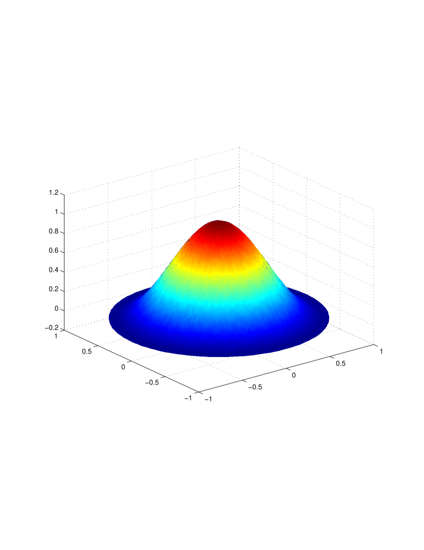
$\kappa\in\mathopen{[}0,j_{0,1}j_{0,2}\mathclose{[}$

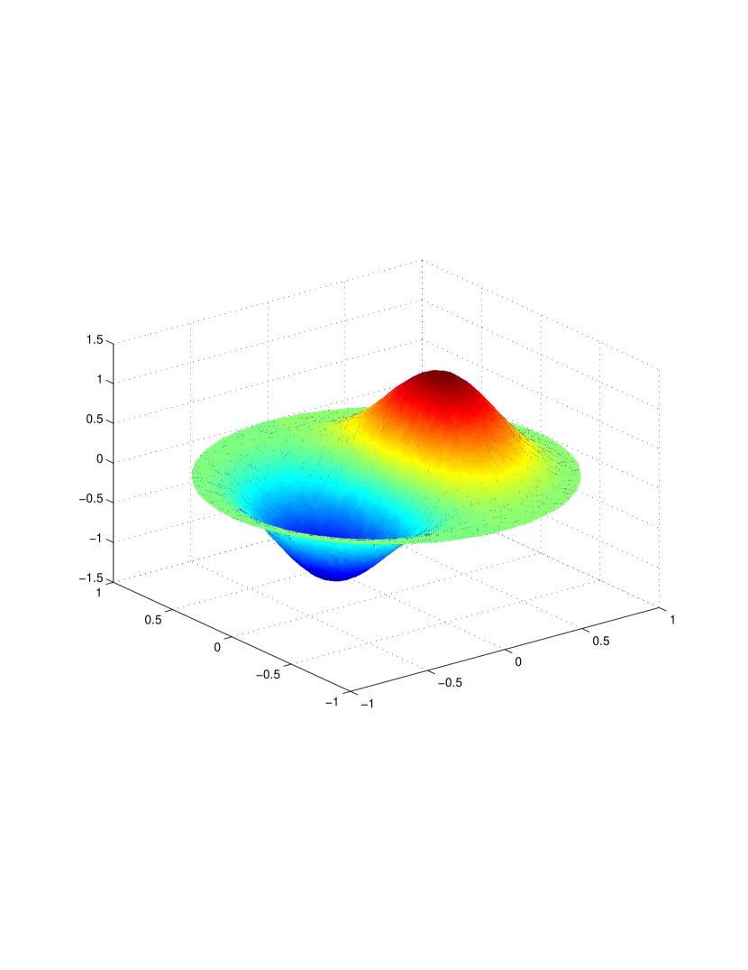
$\kappa\in\mathopen{]}j_{0,1}j_{0,2},\,j_{1,1}j_{1,2}\mathclose{[}$

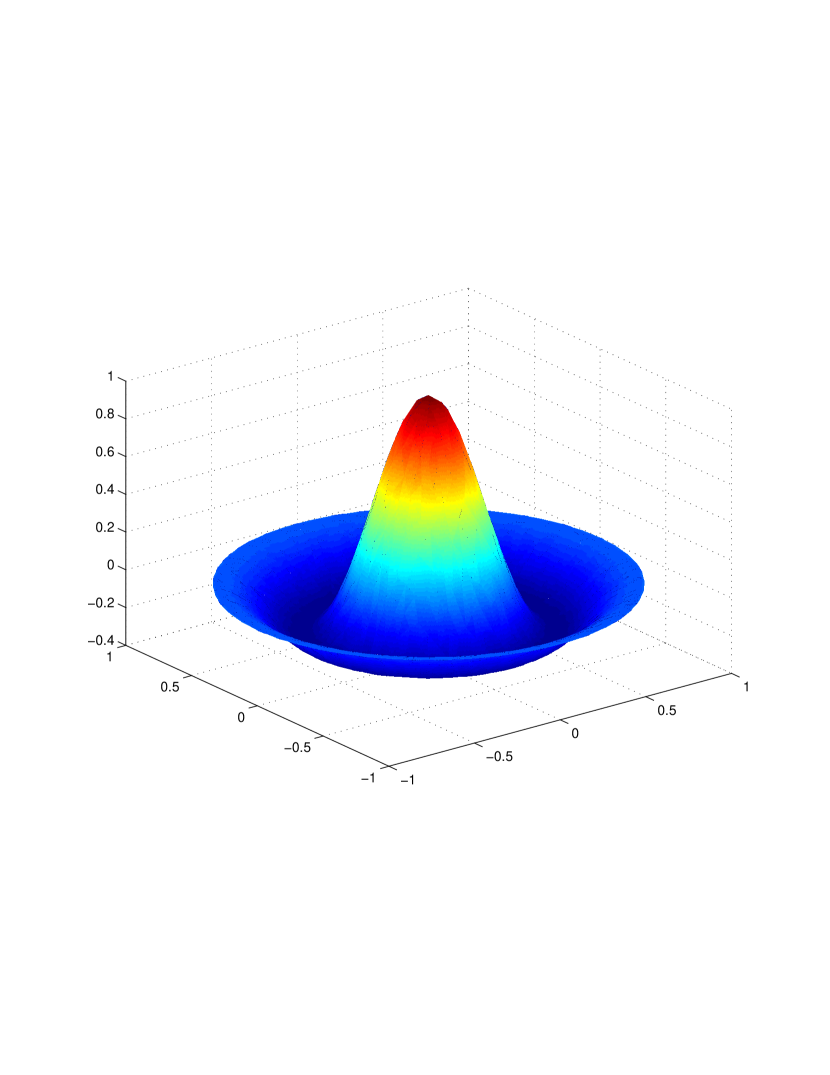
$\kappa\in\mathopen{]}j_{1,1}j_{1,2},\,j_{0,2}j_{0,3}\mathclose{[}$

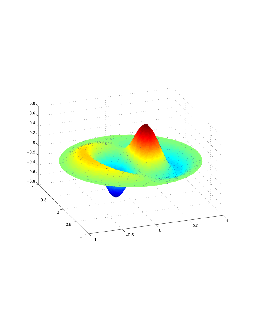
$\kappa\in\mathopen{]}j_{0,2}j_{0,3},\,j_{1,2}j_{1,3}\mathclose{[}$

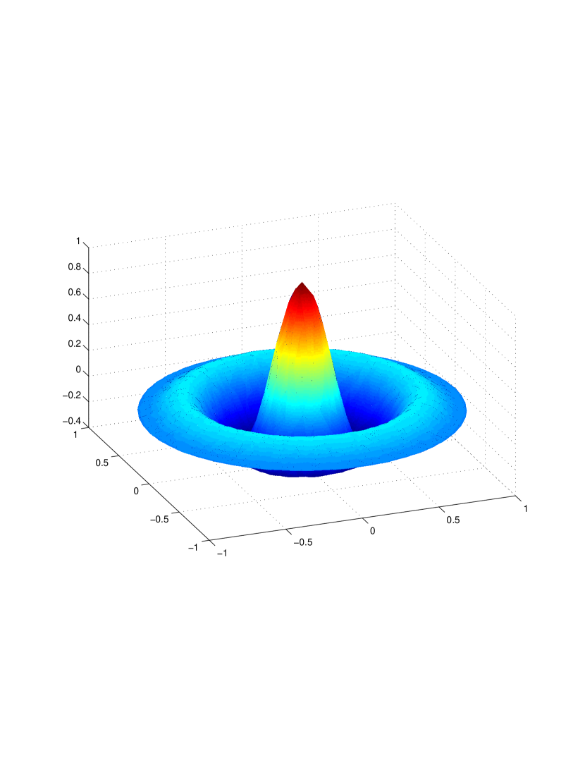
$\kappa\in\mathopen{]}j_{1,2}j_{1,3},\,j_{0,3}j_{0,4}\mathclose{[}$

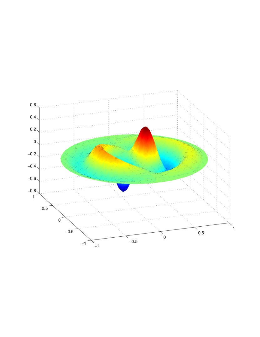
$\kappa\in\mathopen{]}j_{0,3}j_{0,4},\,j_{1,3}j_{1,4}\mathclose{[}$

Figure 1: Graphs of $\varphi_{1}$ for various values of $\kappa$.

In this paper, we use the following notations. The set of natural numbers is denoted $\mathbb{N}=\{0,1,2,\ldots\}$, the set of positive integers is $\mathbb{N}^{*}=\{1,2,\ldots\}$, and $j_{\nu,\ell}$, $\ell\in\mathbb{N}^{*}$ denotes the $\ell$-th positive root of $J_{\nu}$, the Bessel function of the First Kind of order $\nu$.

2 Preliminaries

Given two complex numbers $\alpha$, $\beta$, we look for special solutions $u$ to the equation

$$(\Delta+\alpha^{2})(\Delta+\beta^{2})u=0.$$ (2.1)

Such an equation is equivalent to

$$\Delta^{2}u+(\alpha^{2}+\beta^{2})\Delta u+\alpha^{2}\beta^{2}u=0.$$ (2.2)

Hence if we look for a solution to

$$\Delta^{2}u+\kappa^{2}\,u=-\lambda\Delta u$$ (2.3)

with $\kappa\geqslant 0$ fixed, it suffices to take $\alpha\beta=\kappa$ and $\alpha^{2}+\beta^{2}=\lambda$.

Given that we work in two dimensions, we use the antsatz $u(r,\theta)=R(r)\operatorname{e}^{{\mathbf{i}}k\theta}$ with $k\in\mathbb{Z}$, where $(r,\theta)$ are the polar coordinates, and notice that (2.1) is equivalent to the fourth order differential equation (in $\partial_{r}$)

$$L(\partial_{r},r,\alpha,\beta,\mathopen{|}k\mathclose{|})R=0.$$ (2.4)

We write $L(\partial_{r},r,\alpha,\beta,\mathopen{|}k\mathclose{|})$ to emphasize that the coefficients of the differential operator depend continuously on $r$, $\alpha$, $\beta$ and that the sign of $k$ does not matter. Hence by the theory of ordinary differential equations, $L$ has four linearly independent solutions. To find them it suffices to notice that

$$(\Delta+\alpha^{2})u=0\quad\Rightarrow\quad(\Delta+\alpha^{2})(\Delta+\beta^{2})u=0.$$

Thus if

$$(\Delta+\alpha^{2})\bigl{(}R(r)\operatorname{e}^{{\mathbf{i}}k\theta}\bigr{)}=0$$ (2.5)

then $R$ is a solution to (2.4). But a solution to (2.5) is simpler to find. Indeed then $R$ satisfies the Bessel equation

$$(r\partial_{r})^{2}R+\alpha^{2}r^{2}R=k^{2}R.$$

Hence if $\alpha\neq 0$, $R$ is a linear combination of $J_{|k|}(\alpha r)$ and of $Y_{|k|}(\alpha r)$. On the contrary if $\alpha=0$ and $k\not=0$, then $R$ is a linear combination of $r^{k}$ and of $r^{-k}$ while $R$ is a linear combination of $1$ and $\log r$ when $\alpha=0$ and $k=0$.

We have therefore proved the following result:

Lemma 2.1.

Let $k\in\mathbb{Z}$.

1. If $\alpha\neq\beta$ both non-zero, then the four linearly independent solutions to (2.4) are $J_{|k|}(\alpha r)$, $Y_{|k|}(\alpha r)$, $J_{|k|}(\beta r)$, $Y_{|k|}(\beta r)$.

2. If $\alpha\neq 0$ and $\beta=0$, then the four linearly independent solutions to (2.4) are $J_{|k|}(\alpha r)$, $Y_{|k|}(\alpha r)$, $r^{k}$, $r^{-k}$ if $k\neq 0$ and $J_{|k|}(\alpha r)$, $Y_{|k|}(\alpha r)$, $1$, $\log r$ if $k=0$.

3. If $\alpha=\beta\neq 0$, then the four linearly independent solutions to (2.4) are $J_{|k|}(\alpha r)$, $Y_{|k|}(\alpha r)$, $rJ^{\prime}_{|k|}(\alpha r)$, $rY^{\prime}_{|k|}(\alpha r)$.

Proof.

The first two points were already treated before, the linear independence coming easily from the asymptotic behavior of the Bessel functions and their derivatives at $0$. For the third case, it suffices to notice that taking $\gamma\neq\alpha$, we see that

$$\frac{J_{|k|}(\alpha r)-J_{|k|}(\gamma r)}{\alpha-\gamma}$$

is a solution of

$$L(\partial_{r},r,\alpha,\gamma,\mathopen{|}k\mathclose{|})R=0.$$

Letting $\gamma$ tend to $\alpha$, we prove that $R(r)=rJ^{\prime}_{|k|}(\alpha r)$ is a solution of

$$L(\partial_{r},r,\alpha,\alpha,\mathopen{|}k\mathclose{|})R=0.$$

The same argument holds for $Y_{\mathopen{|}k\mathclose{|}}(\alpha r)$. ∎

3 Eigenvalues in the case $\kappa=0$

Here we want to characterize the full spectrum of the buckling problem with $\kappa=0$ on the unit disk. In other words, we look for a non-trivial $u$ and $\lambda>0$ such that

$$\begin{cases}\Delta^{2}u=-\lambda\Delta u&\text{ in }D_{1},\\ u=\partial_{r}u=0&\text{ on }\partial D_{1},\end{cases}$$ (3.1)

where $D_{1}=\bigl{\{}x\in{\mathbb{R}}^{2}\bigm{|}\mathopen{|}x\mathclose{|}<1\bigr{\}}$. According to the previous section, we look for solutions $u$ in the form

$$u=R(r)\operatorname{e}^{{\mathbf{i}}k\theta},\qquad\text{with }k\in\mathbb{Z},$$

to equation (2.1) with $\alpha=\sqrt{\lambda}$ and $\beta=0$. From Lemma 2.1, we see that

$$R(r)=cr^{|k|}+dJ_{|k|}(\alpha r),$$

for some real numbers $c$ and $d$ (since $R$ and $R^{\prime}$ are bounded around $r=0$). Hence the Dirichlet boundary conditions from (3.1) yield

$$\begin{cases}c+dJ_{|k|}(\alpha)=0,\\[3.0pt] c|k|+d\alpha J^{\prime}_{|k|}(\alpha)=0.\end{cases}$$

This $2\times 2$ system has a non trivial solution if and only if its determinant is zero, namely

$$\alpha J^{\prime}_{|k|}(\alpha)-|k|J_{|k|}(\alpha)=0.$$ (3.2)

If a solution $\alpha$ exists (see Lemma 3.1 below), then $R$ has the form

$$R(r)=d\bigl{(}-J_{|k|}(\alpha)r^{|k|}+J_{|k|}(\alpha r)\bigr{)},$$

for some $d\neq 0$.

Lemma 3.1.

For all $k\in\mathbb{N}$, there exists an increasing sequence $\alpha_{k,\ell}>0$, with $\ell\in{\mathbb{N}}^{*}$, of solutions to (3.2). This sequence is formed by the positive zeros of $J_{k+1}$.

Proof.

For $k\geqslant 0$, we use the formula (A.3) to find that

$$\alpha J^{\prime}_{k}(\alpha)-kJ_{k}(\alpha)=-\alpha J_{k+1}(\alpha).$$

Therefore $\alpha>0$ is a solution of (3.2) if and only if $J_{k+1}(\alpha)=0$. ∎

We are ready to state the following result.

Theorem 3.2.

The spectrum of the buckling problem with $\kappa=0$ is given by $\bigl{\{}\lambda_{k,\ell}:=j_{|k|+1,\ell}^{2}\bigm{|}\ell\in{\mathbb{N}}^{*},\ k\in\mathbb{Z}\bigr{\}}$. A basis of the eigenfunctions is given by

$$(r,\theta)\mapsto-J_{0}(j_{1,\ell})+J_{0}(j_{1,\ell}\,r)$$

giving rise to the eigenvalue $\lambda_{0,\ell}$ and

$$(r,\theta)\mapsto\bigl{(}-J_{|k|}(j_{|k|+1,\ell})r^{|k|}+J_{|k|}(j_{|k|+1,\ell}\,r)\bigr{)}\operatorname{e}^{{\mathbf{i}}k\theta},\quad k\neq 0,$$

giving rise to the eigenvalue $\lambda_{k,\ell}$.

Proof.

We have already showed that all $j_{|k|+1,\ell}^{2}$ are eigenvalues of the operator with the corresponding eigenvectors. It then remains to prove that we have found all eigenvalues. The reason comes essentially from the fact that the functions $(\operatorname{e}^{{\mathbf{i}}k\theta})_{k\in\mathbb{Z}}$ form an orthonormal basis of $L^{2}\bigl{(}\mathopen{]}0,2\pi\mathclose{[}\bigr{)}$. Indeed let $(u,\lambda)$ be a solution to (3.1). We write

$$u=\sum_{k\in\mathbb{Z}}u_{k}(r)\operatorname{e}^{{\mathbf{i}}k\theta},$$

with

$$\forall r>0,\quad u_{k}(r)=\int_{0}^{2\pi}u(r,\theta)\operatorname{e}^{-{\mathbf{i}}k\theta}\,\mathrm{d}\theta$$

(this integral makes sense because $u$ is smooth). Now we check that

$$\forall k\in\mathbb{Z},\quad L(\partial_{r},r,\sqrt{\lambda},0,\mathopen{|}k\mathclose{|})u_{k}=0.$$ (3.3)

Indeed using the differential equation in (3.1), we see that

$$\forall r>0,\quad 0=\int_{0}^{2\pi}(\Delta^{2}+\lambda\Delta)u(r,\theta)\cdot\operatorname{e}^{-{\mathbf{i}}k\theta}\,\mathrm{d}\theta.$$

Writing the operator $\Delta$ and $\Delta^{2}$ in polar coordinates and integrating by parts in $\theta$, we see that the previous identity is equivalent to (3.3). At this stage we use point 2 of Lemma 2.1 to deduce that $u_{k}$ is a linear combination of $r^{|k|}$ and of $J_{|k|}(\sqrt{\lambda}\,r)$ (due to the regularity of $u_{k}$ at $r=0$).

We therefore deduce that $\lambda$ has to be a root of (3.2) and hence $\lambda=\lambda_{k,\ell}$, for some $k\in\mathbb{Z}$ and $\ell\in\mathbb{N}^{*}$, and $u$ is a linear combination of the eigenfunctions given in the statement of this Theorem. ∎

4 Eigenvalues in the case $\kappa>0$

In this section we characterize the eigenfunctions of the buckling problem with $\kappa>0$ on the unit disk $D_{1}$. In other words, we look for a non-trivial $u$ and $\lambda>0$ solving (1.2).

First observe that $\lambda_{1}\geqslant 2\kappa$. As $\int_{D_{1}}(\Delta u+\kappa u)^{2}\geqslant 0$, we have

$$\int_{D_{1}}(|\Delta u|^{2}+\kappa^{2}u^{2})\geqslant-2\kappa\int_{D_{1}}\Delta u\,u=2\kappa\int_{D_{1}}|\nabla u|^{2}.$$

This implies that

$$\lambda_{1}=\inf_{u\in H^{2}_{0}(\Omega)\setminus\{0\}}\frac{\int_{D_{1}}(|\Delta u|^{2}+\kappa^{2}u^{2})}{\int_{D_{1}}|\nabla u|^{2}}\geqslant 2\kappa.$$

As a consequence, we can write (1.2) under the form (2.1) with $\alpha$ and $\beta$ positive real numbers satisfying $\alpha\beta=\kappa$ and $\alpha^{2}+\beta^{2}=\lambda$. Following the same strategy as before, we look for solutions $u=R(r)\operatorname{e}^{{\mathbf{i}}k\theta}$ with $k\in\mathbb{Z}$. Again due to the regularity of $u$ at zero and eliminating $\beta={\kappa}/{\alpha}$, we deduce that, if $\alpha\neq{\kappa}/{\alpha}$, $R$ is in the form

$$R(r)=cJ_{|k|}(\alpha r)+dJ_{|k|}\Bigl{(}\frac{\kappa}{\alpha}r\Bigr{)},$$ (4.1)

for some $c,d\in{\mathbb{R}}$. If instead $\alpha={\kappa}/{\alpha}$ (i.e., $\alpha=\sqrt{\kappa}$),

$$R(r)=cJ_{|k|}(\sqrt{\kappa}r)+drJ^{\prime}_{|k|}(\sqrt{\kappa}r),$$ (4.2)

with $c,d\in{\mathbb{R}}$.

Lemma 4.1.

Let $k\in\mathbb{N}$.

1. The function $\displaystyle\tilde{H}_{k}:\mathopen{]}0,+\infty\mathclose{[}\to{\mathbb{R}}$ defined by

   $$\tilde{H}_{k}(z):=(z^{2}-k^{2})\bigl{(}J_{k}(z)\bigr{)}^{2}+z^{2}\bigl{(}J_{k}^{\prime}(z)\bigr{)}^{2}$$ (4.3)

   is positive and increasing.

2. The function

   $$H_{k}:\mathopen{]}0,+\infty\mathclose{[}\setminus\bigl{\{}j_{k,\ell}\bigm{|}\ell\in\mathbb{N}^{*}\bigr{\}}\to{\mathbb{R}}:z\mapsto\frac{zJ^{\prime}_{k}(z)}{J_{k}(z)}$$

   has a negative derivative

   $$H^{\prime}_{k}(z)=\frac{-\tilde{H}_{k}(z)}{zJ_{k}^{2}(z)}$$ (4.4)

   and thus is decreasing between any two consecutive roots of $J_{k}$. Moreover, for any $\ell\geqslant 1$,

   $$\lim_{z\xrightarrow{>}j_{k,\ell}}H_{k}(z)=+\infty\qquad\text{and}\qquad\lim_{z\xrightarrow{<}j_{k,\ell+1}}H_{k}(z)=-\infty.$$

Proof.

Let $\tilde{H}_{k}$ be defined by (4.3). Differentiating $\tilde{H}_{k}$ and using the equation satisfied by Bessel functions (A.5) gives $\tilde{H}_{k}^{\prime}(z)=2zJ_{k}^{2}(z)$ which is positive for all $z>0$ except at the (isolated) roots of $J_{k}$. Since $\tilde{H}_{k}(0)=0$, this proves the result concerning $\tilde{H}_{k}$.

Using again the differential equation satisfied by Bessel functions (A.5), one easily gets (4.4). Since $\tilde{H}_{k}>0$, the function $H_{k}$ decreases between two consecutive roots of $J_{k}$. Hence the limits are easy to compute once one remarks that the numerator of $H_{k}(z)$ does not vanish at $z=j_{k,m}$ for any $m$ because the positive roots of $J_{k}$ are simple. ∎

Proposition 4.2.

The eigenfunctions of the differential equation (1.2) are of the form $u=R(r)\operatorname{e}^{{\mathbf{i}}k\theta}$ with $k\in\mathbb{Z}$ and $R$ given by (4.1), where $\alpha\neq\sqrt{\kappa}$ and $\alpha$ is a positive solution of

$$F_{k}(\alpha):=\frac{\kappa}{\alpha}J_{|k|}(\alpha)J^{\prime}_{|k|}\Bigl{(}\frac{\kappa}{\alpha}\Bigr{)}-\alpha J_{|k|}\Bigl{(}\frac{\kappa}{\alpha}\Bigr{)}J^{\prime}_{|k|}(\alpha)=0.$$ (4.5)

The corresponding eigenvalue is $\lambda=\alpha^{2}+{\kappa^{2}}/{\alpha^{2}}$.

Proof.

First observe that, in the case $\alpha=\sqrt{\kappa}$, there exists a non-trivial function of the form (4.2) satisfying the boundary conditions at $r=1$ if and only if the system

$$\begin{cases}c\,J_{\mathopen{|}k\mathclose{|}}(\sqrt{\kappa})+d\,J_{\mathopen{|}k\mathclose{|}}^{\prime}(\sqrt{\kappa})=0\\[1.5pt] c\,\sqrt{\kappa}\,J_{\mathopen{|}k\mathclose{|}}^{\prime}(\sqrt{\kappa})+d\bigl{(}J_{\mathopen{|}k\mathclose{|}}^{\prime}(\sqrt{\kappa})+\sqrt{\kappa}\,J_{\mathopen{|}k\mathclose{|}}^{\prime\prime}(\sqrt{\kappa})\bigr{)}=0\end{cases}$$

has a non trivial solution $(c,d)$. This holds if and only if $\alpha=\sqrt{\kappa}$ is a solution of

$$D_{k}(\alpha):=J_{|k|}(\alpha)\bigl{(}J^{\prime}_{|k|}(\alpha)+\alpha\,J^{\prime\prime}_{|k|}(\alpha)\bigr{)}-\alpha\bigl{(}J^{\prime}_{|k|}(\alpha)\bigr{)}^{2}=0.$$ (4.6)

Note that, for all $\alpha>0$, using the equation (A.5) satisfied by Bessel functions, $D_{k}(\alpha)=-\frac{1}{\alpha}\tilde{H}_{\mathopen{|}k\mathclose{|}}(\alpha)<0$ where $\tilde{H}_{\mathopen{|}k\mathclose{|}}$ is defined by (4.3). Consequently (4.6) possesses no solution $\alpha>0$.

In the case (4.1), the boundary conditions at $r=1$ lead to the system

$$\begin{cases}c\,J_{|k|}(\alpha)+d\,J_{|k|}\bigl{(}\frac{\kappa}{\alpha}\bigr{)}=0,\\[3.0pt] c\,\alpha J^{\prime}_{|k|}(\alpha)+d\,\frac{\kappa}{\alpha}J^{\prime}_{|k|}\bigl{(}\frac{\kappa}{\alpha}\bigr{)}=0.\end{cases}$$ (4.7)

This $2\times 2$ system has a non-trivial solution if and only if its determinant is equal to zero, namely if and only if (4.5) is satisfied.

The same arguments than the ones used in Theorem 3.2 allow to conclude that no other eigenvalues exist. ∎

Theorem 4.3.

For all $k\in\mathbb{N}$ and $\kappa>0$, the roots of $F_{k}$ (defined by (4.5)) can be ordered as an increasing sequence $\alpha_{k,\ell}=\alpha_{k,\ell}(\kappa)>0$, with $\ell\in{\mathbb{Z}}$, such that

$$\forall\ell\geqslant 0,\qquad\alpha_{k,-\ell}=\frac{\kappa}{\alpha_{k,\ell}},$$

$$\alpha_{k,0}=\sqrt{\kappa}\quad\text{and}\quad\forall\ell>0,\quad\alpha_{k,\ell}>\sqrt{\kappa}>\alpha_{k,-\ell}\,,$$

$$\alpha_{k,\ell}\to+\infty\text{ as }\ell\to+\infty,$$

$$\alpha_{k,\ell}\to 0\text{ as }\ell\to-\infty.$$

Each $\ell\neq 0$ gives rise to the eigenvalue

$$\lambda_{k,\ell}=\alpha_{k,\ell}^{2}+\frac{\kappa^{2}}{\alpha_{k,\ell}^{2}}=\alpha_{k,\ell}^{2}+\alpha_{k,-\ell}^{2}\,,$$ (4.8)

and a corresponding eigenfunction of the form $R_{k,\ell}(r)\operatorname{e}^{{\mathbf{i}}k\theta}$ with

$$R_{k,\ell}(r)=cJ_{k}(\alpha_{k,\ell}\,r)+dJ_{k}(\alpha_{k,-\ell}\,r),$$

and $c,d$ solutions to (4.7) with $\alpha=\alpha_{k,\ell}$.

Proof.

First notice that

$$\forall\alpha>0,\quad F_{k}\Bigl{(}\frac{\kappa}{\alpha}\Bigr{)}=-F_{k}(\alpha),$$

where $F_{k}$ is defined in (4.5). As a consequence, $F_{k}(\sqrt{\kappa})=0$ and we set $\alpha_{k,0}:=\sqrt{\kappa}$. Moreover it suffices to find the roots of $F_{k}$ in $\mathopen{]}\sqrt{\kappa},+\infty\mathclose{[}$. The function $F_{k}$ being continuous on $\mathopen{]}0,\infty\mathclose{[}$, it will possess infinitely many roots provided it changes sign infinitely many times when $\alpha\to+\infty$.

Formula (A.3) implies that,

$$F_{k}(\alpha)=\alpha J_{k}\Bigl{(}\frac{\kappa}{\alpha}\Bigr{)}J_{k+1}(\alpha)-\frac{\kappa}{\alpha}J_{k}(\alpha)J_{k+1}\Bigl{(}\frac{\kappa}{\alpha}\Bigr{)}.$$

Hence, noting that $\kappa/\alpha=o(1)$, if $\alpha\to\infty$, formulas (A.6) and (A.7) imply that

$$F_{k}(\alpha)=\sqrt{\frac{2\alpha}{\pi}}\frac{1}{k!}\Bigl{(}\frac{\kappa}{2\alpha}\Bigr{)}^{k}\Bigl{(}\cos\bigl{(}\alpha-\tfrac{2k+3}{4}\pi\bigr{)}+o(1)\Bigr{)}\quad\text{as }\alpha\to+\infty.$$

Thus $F_{k}$ oscillates an infinite number of times as $\alpha\to+\infty$. This yields the sequence of $\alpha_{k,\ell}>0$ with $\ell>0$.

Observe that the only possible accumulation points are $0$ and $+\infty$ as otherwise the corresponding eigenvalues $\lambda_{k,\ell}=\alpha_{k,\ell}^{2}+\kappa^{2}/\alpha_{k,\ell}^{2}$ would have a finite accumulation point which contradicts the variational theory of eigenvalues. ∎

In order to better understand the behaviour of the eigenvalues and of the corresponding eigenfunctions, we will now study the functions $\alpha_{k,\ell}$.

Lemma 4.4.

For all $k\in\mathbb{N}$ and $\ell\in\mathbb{Z}$, the function $\alpha_{k,\ell}:\mathopen{]}0,+\infty\mathclose{[}\to{\mathbb{R}}:\kappa\mapsto\alpha_{k,\ell}(\kappa)$ is of class ${\mathcal{C}}^{1}$ and $\partial_{\kappa}\alpha_{k,\ell}>0$.

Proof.

Let us note $F_{k}(\alpha,\kappa)$ the function $F_{k}(\alpha)$ defined by (4.5) where we have explicited the dependence on $\kappa$. The assertion will result from the Implicit Function Theorem. Let us fix $k\in\mathbb{N}$, $\kappa^{*}>0$ and $\alpha^{*}=\alpha_{k,\ell}(\kappa^{*})>0$ and distinguish two cases.

• If $J_{k}(\alpha^{*})=0$ (resp. $J_{k}(\frac{\kappa^{*}}{\alpha^{*}})=0$) then $J_{k}^{\prime}(\alpha^{*})\neq 0$ (resp. $J_{k}^{\prime}(\frac{\kappa^{*}}{\alpha^{*}})\neq 0$) because the roots of the Bessel functions are simple. But then, the fact that $F_{k}(\alpha^{*},\kappa^{*})=0$ implies that $J_{k}(\frac{\kappa^{*}}{\alpha^{*}})=0$ (resp. $J_{k}(\alpha^{*})=0$). A direct computation, using the fact that both $J_{k}(\alpha^{*})$ and $J_{k}(\frac{\kappa^{*}}{\alpha^{*}})$ vanish, shows

  $$\partial_{\kappa}F_{k}(\alpha^{*},\kappa^{*}) =-J^{\prime}_{k}(\alpha^{*})J^{\prime}_{k}\Bigl{(}\frac{\kappa^{*}}{\alpha^{*}}\Bigr{)},$$

  $$\partial_{\alpha}F_{k}(\alpha^{*},\kappa^{*}) =2\frac{\kappa^{*}}{\alpha^{*}}J^{\prime}_{k}(\alpha^{*})J^{\prime}_{k}\Bigl{(}\frac{\kappa^{*}}{\alpha^{*}}\Bigr{)}\neq 0.$$

  Therefore the Implicit Function Theorem implies that there exists ${\mathcal{C}}^{1}$ curve $\beta_{\ell}$ around $\kappa^{*}$ such that, in a neighbourhood of $(\alpha^{*},\kappa^{*})$,

  $$F_{k}(\alpha,\kappa)=0\text{ if and only if }\alpha=\beta_{\ell}(\kappa).$$

  Moreover

  $$\partial_{\kappa}\beta_{\ell}(\kappa^{*})=-\frac{\partial_{\kappa}F_{k}(\alpha^{*},\kappa^{*})}{\partial_{\alpha}F_{k}(\alpha^{*},\kappa^{*})}=\frac{\alpha^{*}}{2\kappa^{*}}>0.$$

• Let us now suppose that $J_{k}(\alpha^{*})\neq 0$ and $J_{k}(\frac{\kappa^{*}}{\alpha^{*}})\neq 0$. Around such $(\alpha^{*},\kappa^{*})$, one can write

  $$F_{k}(\alpha,\kappa)=J_{k}(\alpha)J_{k}\Bigl{(}\frac{\kappa}{\alpha}\Bigr{)}\tilde{F}_{k}(\alpha,\kappa)\quad\text{with}\quad\tilde{F}_{k}(\alpha,\kappa):=H_{k}\Bigl{(}\frac{\kappa}{\alpha}\Bigr{)}-H_{k}(\alpha),$$

  where $H_{k}$ is defined in Lemma 4.1. Using Lemma 4.1, one deduces

  $$\partial_{\kappa}\tilde{F}_{k}(\alpha,\kappa) =\frac{1}{\alpha}H^{\prime}_{k}\Bigl{(}\frac{\kappa}{\alpha}\Bigr{)}<0,$$

  $$\partial_{\alpha}\tilde{F}_{k}(\alpha,\kappa) =-\frac{\kappa}{\alpha^{2}}H^{\prime}_{k}\Bigl{(}\frac{\kappa}{\alpha}\Bigr{)}-H^{\prime}_{k}(\alpha)>0.$$

  Therefore the Implicit Function Theorem applies to $\tilde{F}_{k}$ and there exists a ${\mathcal{C}}^{1}$ curve $\beta_{\ell}$ defined around $\kappa^{*}$ such that, in a neighbourhood of $(\alpha^{*},\kappa^{*})$,

  $$F_{k}(\alpha,\kappa)=0\text{ if and only if }\alpha=\beta_{\ell}(\kappa).$$

  Moreover

  $$\partial_{\kappa}\beta_{\ell}(\kappa^{*})=-\frac{\partial_{\kappa}\tilde{F}_{k}(\alpha^{*},\kappa^{*})}{\mathstrut\partial_{\alpha}\tilde{F}_{k}(\alpha^{*},\kappa^{*})}>0.$$

This argument can be done for all $\ell$. Thus, for all $\ell$, we have a ${\mathcal{C}}^{1}$-curve emanating from $\alpha_{k,\ell}(\kappa^{*})$ such that, in a neighbourhood $U_{\ell}$ of $(\alpha_{k,\ell}(\kappa^{*}),\kappa^{*})$,

$$F_{k}(\alpha,\kappa)=0\text{ if and only if }\alpha=\beta_{\ell}(\kappa).$$

Moreover, as $F_{k}(\alpha,\kappa^{*})\not=0$ for $\alpha\notin\{\alpha_{k,\ell}(\kappa^{*})\mid\ell\in\mathbb{Z}\}$, the continuity of $F_{k}$ implies the existence of a neighbourhood $V_{\ell}$ of $\{(\alpha,\kappa^{*})\mid\alpha_{k,\ell-1}(\kappa^{*})<\alpha<\alpha_{k,\ell}(\kappa^{*}),\linebreak[2]\ (\alpha,\kappa^{*})\notin U_{\ell-1}\cup U_{\ell}\}$ such that $F_{k}(\alpha,\kappa)\neq 0$ for $(\alpha,\kappa)\in V_{\ell}$. In this way, one shows that there is a neighbourhood $V$ of $[\sqrt{\kappa^{*}},\alpha^{*}]$ and $W$ of $\kappa^{*}$ such that, for all $(\alpha,\kappa)\in V\times W$,

$$F_{k}(\alpha,\kappa)=0\quad\text{if and only if}\quad\alpha=\beta_{\ell^{\prime}}(\kappa)\text{ for some }0\leqslant\ell^{\prime}\leqslant\ell.$$

Shrinking $W$ if necessary, one can assume the curves $\beta_{0},\beta_{1},\dotsc,\beta_{\ell}$ do not cross each other. For any given $\kappa\in W$, it then suffices to count the number of curves one meets to reach the one emanating from $(\alpha^{*},\kappa^{*})$ starting with $\alpha=\alpha_{k,0}(\kappa)=\sqrt{\kappa}$ to establish that

$$\forall\kappa\in V,\quad\beta_{\ell}(\kappa)=\alpha_{k,\ell}(\kappa),$$

whence the desired result. ∎

Lemma 4.5.

Let $k\in\mathbb{N}$ and $\ell>0$. As $\kappa\to 0$, $\alpha_{k,\ell}(\kappa)\to j_{k+1,\ell}$. Consequently $\alpha_{k,-\ell}(\kappa)=\kappa/\alpha_{k,\ell}(\kappa)\to 0$ if $\kappa\to 0$.

Proof.

Without loss of generality, we can restrict $\kappa$ to $\mathopen{]}0,j_{k,1}^{2}\mathclose{[}$ so that, as we will only consider $\alpha>\sqrt{\kappa}$, we have $\kappa/\alpha<\sqrt{\kappa}<j_{k,1}$ and thus $J_{k}(\kappa/\alpha)\neq 0$. For such $\kappa$, one also has that $J_{k}(\alpha_{k,\ell})\neq 0$ (otherwise that would imply $J_{k}(\kappa/\alpha_{k,\ell})=0$, see the proof of Lemma 4.4) and so $\alpha_{k,\ell}(\kappa)\neq j_{k,m}$ for any $m\geqslant 1$.

According to formulas (A.7) and (A.3), one has as $z\to 0$,

$$\begin{array}[]{cl}\displaystyle J_{k}(z)=\frac{1+o(1)}{k!}(\tfrac{1}{2}z)^{k},&\\[8.53581pt] \displaystyle J^{\prime}_{k}(z)=-J_{k+1}(z)+\frac{k}{z}J_{k}(z)=\frac{1+o(1)}{2(k-1)!}(\tfrac{1}{2}z)^{k-1}&\qquad\text{if }k\not=0,\\[8.53581pt] \displaystyle J_{0}^{\prime}(z)=-(1+o(1))\frac{z}{2}.&\end{array}$$

This implies that

$$\lim_{z\to 0}H_{k}(z)=k$$ (4.9)

where $H_{k}$ is defined in Lemma 4.1, and so, restricting further $\kappa$, one can assume $H_{k}(\kappa/\alpha)$ is bounded (as $0<\kappa/\alpha<\sqrt{\kappa}$).

Let us start by showing that

$$j_{k,1}<\alpha_{k,1}(\kappa)<j_{k,2}.$$

As $\sqrt{\kappa}<\alpha_{k,1}(\kappa)$, in order to establish the left inequality, it suffices to show that for all $\alpha\in\mathopen{]}\sqrt{\kappa},j_{k,1}\mathclose{[}$, $F_{k}(\alpha)\neq 0$ ($\alpha_{k,1}\neq j_{k,1}$ was established above). But, for $\alpha$ below the first root of $J_{k}$, $F_{k}(\alpha)\neq 0$ is equivalent to $\tilde{F}_{k}(\alpha,\kappa)\neq 0$ where $\tilde{F}_{k}$, defined in the proof of Lemma 4.4, is a smooth function on $\mathopen{]}\sqrt{\kappa},j_{k,1}\mathclose{[}$. The argument is complete if one recalls that $\partial_{\alpha}\tilde{F}_{k}(\alpha,\kappa)>0$ and that $\tilde{F}_{k}(\sqrt{\kappa},\kappa)=0$.

For the right inequality, we first notice that the boundedness of $H_{k}(\kappa/\alpha)$ and Lemma 4.1 imply

$$\lim_{\alpha\xrightarrow{>}j_{k,1}}\tilde{F}_{k}(\alpha,\kappa)=-\infty\quad\text{and}\quad\lim_{\alpha\xrightarrow{<}j_{k,2}}\tilde{F}_{k}(\alpha,\kappa)=+\infty.$$

By continuity and monotonicity, $\tilde{F}_{k}(\alpha,\kappa)$ must possess a unique zero $\alpha\in\mathopen{]}j_{k,1},j_{k,2}\mathclose{[}$. Since we are between two consecutive roots of $J_{k}$, that implies $F_{k}(\alpha)=0$ and thus the desired inequality by definition of $\alpha_{k,1}$.

The same reasoning applies to $\alpha\mapsto\tilde{F}_{k}(\alpha,\kappa)$ on the interval $\mathopen{]}j_{k,\ell},j_{k,\ell+1}\mathclose{[}$, $\ell\geqslant 2$, thereby proving the existence of a unique root of $F_{k}$ in that interval. Counting the number of roots below shows that this root is nothing but $\alpha_{k,\ell}$ therefore establishing that

$$j_{k,\ell}<\alpha_{k,\ell}(\kappa)<j_{k,\ell+1}.$$

Now let us pass to the limit $\kappa\to 0$. Given that $\alpha_{k,\ell}$ is increasing and bounded from below by a positive constant, we have $\alpha_{k,\ell}^{*}:=\lim_{\kappa\xrightarrow{>}0}\alpha_{k,\ell}(\kappa)\in\mathopen{[}j_{k,\ell},j_{k,\ell+1}\mathclose{[}$. Notice that, as $J_{k}\bigl{(}\frac{\kappa}{\alpha_{k,\ell}}\bigr{)}\neq 0$, the equation $F_{k}(\alpha_{k,\ell})=0$ can be rewritten as

$$J_{k}(\alpha_{k,\ell})H_{k}\Bigl{(}\frac{\kappa}{\alpha_{k,\ell}}\Bigr{)}-\alpha_{k,\ell}J^{\prime}_{k}(\alpha_{k,\ell})=0.$$

Passing to the limit $\kappa\to 0$ in this equation yields, by (4.9), $J_{k}(\alpha_{k,\ell}^{*})k-\alpha_{k,\ell}^{*}J^{\prime}_{k}(\alpha_{k,\ell}^{*})=0$ or equivalently, by formula (A.3), $J_{k+1}(\alpha_{k,\ell}^{*})=0$. As $j_{k,\ell}\leqslant\alpha_{k,\ell}^{*}<j_{k,\ell+1}$, the interlacing property of the zeros of Bessel functions (see e.g. (A.8)) implies that $\alpha_{k,\ell}^{*}=j_{k+1,\ell}$. ∎

Lemma 4.6.

For all $k\in\mathbb{N}$ and all $\ell\in\mathbb{Z}$, we have $\displaystyle\lim_{\kappa\to\infty}\alpha_{k,\ell}(\kappa)=+\infty$.

Proof.

This is obvious for $\ell\geqslant 0$ because $\alpha_{k,\ell}(\kappa)\geqslant\sqrt{\kappa}$. Assume on the contrary that there exists $\ell>0$ such that $\lim_{\kappa\to\infty}\alpha_{k,-\ell}(\kappa)<+\infty$ (recall that $\alpha_{k,-\ell}$ is increasing). Hence, there exists $\kappa^{*}>0$ such that, for all $\kappa>\kappa^{*}$, $\alpha_{k,{-\ell}}(\kappa)$ lies between two consecutive roots of $J_{k}$ and of $J_{k}^{\prime}$, i.e., $J_{k}(\alpha_{k,{-\ell}}(\kappa))\not=0$ and $J_{k}^{\prime}(\alpha_{k,{-\ell}}(\kappa))\neq 0$. Because the roots of $J_{k}$ are simple, (4.5) implies that, for all $\kappa>\kappa^{*}$, $J_{k}(\alpha_{k,{\ell}}(\kappa))\not=0$ and $J_{k+1}(\alpha_{k,{\ell}}(\kappa))\neq 0$ (recall that $\alpha_{k,{\ell}}(\kappa)=\kappa/\alpha_{k,{-\ell}}(\kappa)$). This contradicts the fact that $\alpha_{k,{\ell}}$ crosses infinitely many roots of $J_{k}$ because $\alpha_{k,{\ell}}$ is continuous and $\alpha_{k,{\ell}}(\kappa)\xrightarrow[\kappa\to\infty]{}+\infty$. ∎

As shown in Figure 2 and 3, the curves $\alpha_{k,\ell}$ and $\alpha_{k+1,\ell}$ cross each other. In Proposition 4.11 we will characterize their intersection points. This will be done in several steps given by the following lemmas.

Figure 2: Graphs of $\alpha_{k,\ell}$

Lemma 4.7.

Let $k\in\mathbb{N}$. The functions $F_{k}$ and $F_{k+1}$ have a common positive root $\alpha\neq\sqrt{\kappa}$ if and only if there exists positive integers $m$ and $n$ such that $m\neq n$ and

• $\alpha=j_{k,n}$ and $\kappa/\alpha=j_{k,m}$ (thus $\kappa=j_{k,m}\,j_{k,n}$), or

• $\alpha=j_{k+1,n}$ and $\kappa/\alpha=j_{k+1,m}$ (thus $\kappa=j_{k+1,m}\,j_{k+1,n}$).

Proof.

First recall that, using the identity (A.3), we find that

$$F_{k}(\alpha)=\alpha J_{k}\Bigl{(}\frac{\kappa}{\alpha}\Bigr{)}J_{k+1}(\alpha)-\frac{\kappa}{\alpha}J_{k}(\alpha)J_{k+1}\Bigl{(}\frac{\kappa}{\alpha}\Bigr{)}.$$ (4.10)

If instead one uses the identity (A.2), we have

$$F_{k+1}(\alpha)=\frac{\kappa}{\alpha}J_{k}\Bigl{(}\frac{\kappa}{\alpha}\Bigr{)}J_{k+1}(\alpha)-\alpha J_{k}(\alpha)J_{k+1}\Bigl{(}\frac{\kappa}{\alpha}\Bigr{)}.$$ (4.11)

($\Leftarrow$) If $\alpha=j_{k,n}$ and $\kappa/\alpha=j_{k,m}$, one easily see that $F_{k}(\alpha)=0=F_{k+1}(\alpha)$. A similar argument establish this implication when $\alpha=j_{k+1,n}$ and $\kappa/\alpha=j_{k+1,m}$.

($\Rightarrow$) Now let us prove that, if $F_{k}(\alpha)=0=F_{k+1}(\alpha)$ for some $0<\alpha\neq\sqrt{\kappa}$, then $\alpha$ and $\kappa/\alpha$ have the desired values. In view of (4.10)–(4.11), if $F_{k}(\alpha)=0$, one can write

$$0=F_{k+1}(\alpha)=\frac{\kappa^{2}-\alpha^{4}}{\kappa\alpha}J_{k+1}(\alpha)J_{k}\Bigl{(}\frac{\kappa}{\alpha}\Bigr{)}.$$

Two cases can occur:

• $\alpha$ is a root of $J_{k+1}$, i.e., $\alpha=j_{k+1,n}$ for some $n$. Since the zeros of $J_{k}$ and $J_{k+1}$ interlace (see (A.8)), $J_{k}(\alpha)\neq 0$. Then, using the fact that $F_{k}(\alpha)=0$, one deduces that $\kappa/\alpha$ is also a root of $J_{k+1}$, say $j_{k+1,m}$ for some $m$. As $\alpha\neq\sqrt{\kappa}$, one has $n\neq m$.

• $\kappa/\alpha$ is a root of $J_{k}$. A reasoning similar to the first case then shows that $\alpha$ is also a root of $J_{k}$ and the conclusion readily follows. ∎

Figure 3: Mapping of intervals by $\alpha_{k,\ell}$.

Lemma 4.8.

For all $k\in\mathbb{N}$, $\ell\geqslant 1$ and $n\geqslant 1$, we have

$$\alpha_{k,\ell}(j_{k,n}\,j_{k,\ell+n}) =j_{k,\ell+n} =\alpha_{k+1,\ell}(j_{k,n}\,j_{k,\ell+n}),$$

$$\alpha_{k,-\ell}(j_{k,n}\,j_{k,\ell+n}) =j_{k,n} =\alpha_{k+1,-\ell}(j_{k,n}\,j_{k,\ell+n}),$$

$$\alpha_{k,\ell}(j_{k+1,n}\,j_{k+1,\ell+n}) =j_{k+1,\ell+n} =\alpha_{k+1,\ell}(j_{k+1,n}\,j_{k+1,\ell+n}),$$

$$\alpha_{k,-\ell}(j_{k+1,n}\,j_{k+1,\ell+n}) =j_{k+1,n} =\alpha_{k+1,-\ell}(j_{k+1,n}\,j_{k+1,\ell+n}).$$

Proof.

Let us first deal with $\alpha_{k,\pm\ell}$ (left equalities). As $\alpha_{k,\ell}$ is continuous, increasing and satisfies $\alpha_{k,\ell}(\mathopen{]}0,+\infty\mathclose{[})=\mathopen{]}j_{k+1,\ell},+\infty\mathclose{[}$, there exists an increasing sequence $(\kappa_{n})_{n\geqslant 1}$ such that, for all $n\geqslant 1$,

$$\alpha_{k,\ell}(\kappa_{2n-1})=j_{k,\ell+n}\quad\text{and}\quad\alpha_{k,\ell}(\kappa_{2n})=j_{k+1,\ell+n}.$$

In the same way, since $\alpha_{k,-\ell}$ is increasing and $\alpha_{k,-\ell}(\mathopen{]}0,+\infty\mathclose{[})=\mathopen{]}0,+\infty\mathclose{[}$, there exists an increasing sequence $(\tilde{\kappa}_{n})_{n\geqslant 1}$ such that, for all $n\geqslant 1$,

$$\alpha_{k,-\ell}(\tilde{\kappa}_{2n-1})=j_{k,n}\quad\text{and}\quad\alpha_{k,-l}(\tilde{\kappa}_{2n})=j_{k+1,n}.$$

By (4.10), for all roots $\alpha$ of $F_{k}$, $J_{k}(\alpha)=0$ if and only if $J_{k}(\kappa/\alpha)=0$, and so $\{\kappa_{2n-1}\mid n\geqslant 1\}=\{\tilde{\kappa}_{2n-1}\mid n\geqslant 1\}$. Similarly, $\{\kappa_{2n}\mid n\geqslant 1\}=\{\tilde{\kappa}_{2n}\mid n\geqslant 1\}$. Since the sequences are increasing, we conclude that, for all $n\geqslant 1$, $\kappa_{n}=\tilde{\kappa}_{n}$. Moreover, we deduce from $\kappa=\alpha_{k,-\ell}(\kappa)\alpha_{k,\ell}(\kappa)$ that, for all $n\geqslant 1$, $\kappa_{2n-1}=j_{k,n}\,j_{k,\ell+n}$ and $\kappa_{2n}=j_{k+1,n}\,j_{k+1,\ell+n}$. This proves the left hand equalities.

To prove the equalities to the right, let us first show that $j_{k+2,\ell}<j_{k,\ell+1}$. For this, it is enough to prove that $J_{k+2}(j_{k,\ell^{\prime}})$ and $J_{k+2}(j_{k,\ell^{\prime}+1})$ have opposite signs for any $\ell^{\prime}=1,\dotsc,\ell$. Using the relations (A.1) and (A.3), we obtain

$$\begin{split}J_{k+2}(z)&=\frac{2(k+1)}{z}J_{k+1}(z)-J_{k}(z)\\ &=\frac{2(k+1)}{z}\Bigl{(}\frac{k}{z}J_{k}(z)-J_{k}^{\prime}(z)\Bigr{)}-J_{k}(z)\\ &=\Bigl{(}\frac{2(k+1)k}{z^{2}}-1\Bigr{)}J_{k}(z)-\frac{2(k+1)}{z}J_{k}^{\prime}(z).\end{split}$$

Therefore

$$J_{k+2}(j_{k,\ell^{\prime}})\,J_{k+2}(j_{k,\ell^{\prime}+1})=4(k+1)^{2}\frac{J_{k}^{\prime}(j_{k,\ell^{\prime}})J_{k}^{\prime}(j_{k,\ell^{\prime}+1})}{j_{k,\ell^{\prime}}\,j_{k,\ell^{\prime}+1}}$$

which is negative because $j_{k,\ell^{\prime}}$ and $j_{k,\ell^{\prime}+1}$ are two consecutive simple roots of $J_{k}$.

In a similar way to the first part, as $\alpha_{k+1,\ell}$ and $\alpha_{k+1,-\ell}$ are increasing and satisfy $\alpha_{k+1,\ell}(\mathopen{]}0,+\infty\mathclose{[})=\mathopen{]}j_{k+2,\ell},+\infty\mathclose{[}$ and $\alpha_{k+1,-\ell}(\mathopen{]}0,+\infty\mathclose{[})=\mathopen{]}0,+\infty\mathclose{[}$ and as $j_{k,\ell+1}>j_{k+2,\ell}>j_{k+1,\ell}>j_{k,\ell}$, there exist increasing sequences $(\kappa_{n})_{n\geqslant 1}$ and $(\tilde{\kappa}_{n})_{n\geqslant 1}$ such that, for all $n\geqslant 1$,

$$\alpha_{k+1,\ell}(\kappa_{2n-1}) =j_{k,\ell+n} \alpha_{k+1,\ell}(\kappa_{2n}) =j_{k+1,\ell+n},$$ and

$$\alpha_{k+1,-\ell}(\tilde{\kappa}_{2n-1}) =j_{k,n} \alpha_{k+1,-\ell}(\tilde{\kappa}_{2n}) =j_{k+1,n}.$$ and

Now, using (4.11) and arguing as above, we obtain that $\{\kappa_{2n-1}\mid n\geqslant 1\}=\{\tilde{\kappa}_{2n-1}\mid n\geqslant 1\}$ and $\{\kappa_{2n}\mid n\geqslant 1\}=\{\tilde{\kappa}_{2n}\mid n\geqslant 1\}$. As the sequences are increasing, one deduces that $\kappa_{n}=\tilde{\kappa}_{n}$ for all $n$. Finally, from $\kappa=\alpha_{k+1,\ell}(\kappa)\alpha_{k+1,-\ell}(\kappa)$, one gets that, for all $n\geqslant 1$, $\kappa_{2n-1}=j_{k,n}\,j_{k,\ell+n}$ and $\kappa_{2n}=j_{k+1,n}\,j_{k+1,\ell+n}$. ∎

Remark 4.9.

This proof establishes that the positive roots of $J_{k}$ and $J_{k+2}$ interlace (see also [19, Theorem 1]), namely

$$\forall\ell\geqslant 1,\qquad j_{k,\ell}<j_{k+2,\ell}<j_{k,\ell+1}$$

(the first inequality comes from $j_{k,\ell}<j_{k+1,\ell}<j_{k+2,\ell}$).

Remark 4.10.

As a byproduct of the proof, one gets that, for $\ell\geqslant 1$ and $n\geqslant 1$,

$$j_{k,n}j_{k,\ell+n}<j_{k+1,n}j_{k+1,\ell+n}<j_{k,n+1}j_{k,\ell+n+1}.$$ (4.12)

Since the functions $\alpha_{k,\ell}$ are increasing, one immediately deduces that

$$\alpha_{k,\ell}\bigl{(}\mathopen{]}0,j_{k,1}j_{k,\ell+1}\mathclose{[}\bigr{)} =\mathopen{]}j_{k+1,\ell},j_{k,\ell+1}\mathclose{[},$$

$$\alpha_{k+1,\ell}\bigl{(}\mathopen{]}0,j_{k,1}j_{k,\ell+1}\mathclose{[}\bigr{)} =\mathopen{]}j_{k+2,\ell},j_{k,\ell+1}\mathclose{[},$$

$$\alpha_{k,\ell}(I)=\alpha_{k+1,\ell}(I) =\mathopen{]}j_{k,\ell+n},j_{k+1,\ell+n}\mathclose{[}$$

$$\qquad\text{where }I=\mathopen{]}j_{k,n}j_{k,\ell+n},\,j_{k+1,n}j_{k+1,\ell+n}\mathclose{[},$$

$$\alpha_{k,\ell}(I)=\alpha_{k+1,\ell}(I) =\mathopen{]}j_{k+1,\ell+n},j_{k,\ell+n+1}\mathclose{[}$$

$$\qquad\text{where }I=\mathopen{]}j_{k+1,n}j_{k+1,\ell+n},\,j_{k,n+1}j_{k,\ell+n+1}\mathclose{[}.$$

Note further that these properties also yield (see figure 3)

$$\alpha_{k,\ell}(I)=\alpha_{k+1,\ell}(I) =\mathopen{]}j_{k,\ell+n},j_{k,\ell+n+1}\mathclose{[}$$ (4.13)

$$\qquad\text{where }I=\mathopen{]}j_{k,n}j_{k,\ell+n},\,j_{k,n+1}j_{k,\ell+n+1}\mathclose{[}$$

for all $n\geqslant 0$, with the convention that $j_{k,0}:=0$. In the same way, we have

$$\alpha_{k,-\ell}\bigl{(}\mathopen{]}0,j_{k,1}j_{k,\ell+1}\mathclose{[}\bigr{)} =\mathopen{]}0,j_{k,1}\mathclose{[},$$

$$\alpha_{k+1,-\ell}\bigl{(}\mathopen{]}0,j_{k,1}j_{k,\ell+1}\mathclose{[}\bigr{)} =\mathopen{]}0,j_{k,1}\mathclose{[},$$

$$\alpha_{k,-\ell}(I)=\alpha_{k+1,-\ell}(I) =\mathopen{]}j_{k,n},j_{k+1,n}\mathclose{[}$$

$$\qquad\text{where }I=\mathopen{]}j_{k,n}j_{k,\ell+n},\,j_{k+1,n}j_{k+1,\ell+n}\mathclose{[},$$

$$\alpha_{k,-\ell}(I)=\alpha_{k+1,-\ell}(I) =\mathopen{]}j_{k+1,n},j_{k,n+1}\mathclose{[}$$

$$\qquad\text{where }I=\mathopen{]}j_{k+1,n}j_{k+1,\ell+n},\,j_{k,n+1}j_{k,\ell+n+1}\mathclose{[}.$$

and, in particular, for all $$n\geqslant 0$$,

$$\alpha_{k,-\ell}(I)=\alpha_{k+1,-\ell}(I) =\mathopen{]}j_{k,n},j_{k,n+1}\mathclose{[}$$ (4.14)

$$\qquad\text{where }I=\mathopen{]}j_{k,n}j_{k,\ell+n},\,j_{k,n+1}j_{k,\ell+n+1}\mathclose{[}.$$

Proposition 4.11.

Let $k\in\mathbb{N}$ and $\ell\geqslant 1$. The set of $\kappa$ such that $\alpha_{k,\ell}(\kappa)=\alpha_{k+1,\ell}(\kappa)$ is

$$\{j_{k,n}j_{k,\ell+n}\mid n\geqslant 1\}\cup\{j_{k+1,n}j_{k+1,\ell+n}\mid n\geqslant 1\}.$$

Proof.

By Lemma 4.8, we know that the elements of the set $\{j_{k,n}j_{k,\ell+n}\mid n\geqslant 1\}\cup\{j_{k+1,n}j_{k+1,\ell+n}\mid n\geqslant 1\}$ are equality points of $\alpha_{k,\ell}$ and $\alpha_{k+1,\ell}$.

Let us prove that there is no other point where $\alpha_{k,\ell}=\alpha_{k+1,\ell}$. Lemma 4.7 implies that, if $\bar{\kappa}$ is such a point, then $\alpha_{k,\ell}(\bar{\kappa})=\alpha_{k+1,\ell}(\bar{\kappa})=j_{k,m}$ or $\alpha_{k,\ell}(\bar{\kappa})=\alpha_{k+1,\ell}(\bar{\kappa})=j_{k+1,m}$ for some positive integer $m$. In either case, $m>\ell$ because, by Lemmas 4.4 and 4.5, $\alpha_{k+1,\ell}>j_{k+2,\ell}>j_{k+1,\ell}>j_{k,\ell}$. Since $\alpha_{k,\ell}$ is increasing, hence injective, $\bar{\kappa}$ must then necessarily be one of the values given by Lemma 4.8. ∎

We will need also the following result in the next section.

Lemma 4.12.

Let $k\in\mathbb{N}$ and $\ell\in\mathbb{N}\setminus\{0\}$ be fixed. Then the function $\displaystyle g_{k,\ell}:\mathopen{]}0,+\infty\mathclose{[}\to{\mathbb{R}}:\kappa\mapsto\frac{\alpha_{k,\ell}^{2}(\kappa)}{\kappa}$ is decreasing.

Proof.

Direct calculations show $g_{k,\ell}^{\prime}(\kappa)=\frac{\alpha_{k,\ell}(\kappa)}{\kappa^{2}}\bigl{(}2\kappa\alpha_{k,\ell}^{\prime}(\kappa)-\alpha_{k,\ell}(\kappa)\bigr{)}.$ Set

$$G(\kappa):=2\kappa\alpha_{k,\ell}^{\prime}(\kappa)-\alpha_{k,\ell}(\kappa).$$

Because $g_{k,\ell}$ is continuous and the intervals $\mathopen{]}j_{k,n}j_{k,\ell+n},\,j_{k,n+1}j_{k,\ell+n+1}\mathclose{[}$ cover $\mathopen{]}0,+\infty\mathclose{[}$ except for isolated points, it is sufficient to show that, for all $n\geqslant 0$,

$$\forall\kappa\in\mathopen{]}j_{k,n}j_{k,\ell+n},\,j_{k,n+1}j_{k,\ell+n+1}\mathclose{[},\qquad G(\kappa)<0$$

with the convention that $j_{k,0}:=0$. For $\kappa\in\mathopen{]}j_{k,n}j_{k,\ell+n},\,j_{k,n+1}j_{k,\ell+n+1}\mathclose{[}$, by (4.13), $\alpha_{k,\ell}(\kappa)$ is not a root of $J_{k}$ and by the proof of Lemma 4.4, we deduce that

$$G(\kappa)=\alpha\frac{\frac{\kappa}{\alpha}H_{k}^{\prime}(\frac{\kappa}{\alpha})-\alpha H_{k}^{\prime}(\alpha)}{\frac{\kappa}{\alpha}H_{k}^{\prime}(\frac{\kappa}{\alpha})+\alpha H_{k}^{\prime}(\alpha)},$$

where for shortness we have written $\alpha$ instead of $\alpha_{k,\ell}(\kappa)$. Again the fact that $\alpha_{k,\ell}(\kappa)$ and $\frac{\kappa}{\alpha}=\alpha_{k,-\ell}(\kappa)$ are between two consecutive roots of $J_{k}$ allows to apply Lemma 4.1 and deduce that the above denominator is negative. Hence it remains to check that

$$N(\kappa):=\frac{\kappa}{\alpha}H_{k}^{\prime}\Bigl{(}\frac{\kappa}{\alpha}\Bigr{)}-\alpha H_{k}^{\prime}(\alpha)>0,$$

for all $\kappa\in\mathopen{]}j_{k,n}j_{k,\ell+n},\,j_{k,n+1}j_{k,\ell+n+1}\mathclose{[}$. With the help of the identities (4.3) and (4.4), we may transform $N$ into

$$N(\kappa)=\frac{1}{J_{k}^{2}(\alpha)J_{k}^{2}(\frac{\kappa}{\alpha})}\Bigl{[}\Bigl{(}\alpha^{2}-\frac{\kappa^{2}}{\alpha^{2}}\Bigr{)}J_{k}^{2}(\alpha)J_{k}^{2}\Bigl{(}\frac{\kappa}{\alpha}\Bigr{)}\\ +\alpha^{2}\left(J_{k}^{\prime}(\alpha)\right)^{2}J_{k}^{2}\Bigl{(}\frac{\kappa}{\alpha}\Bigr{)}-\frac{\kappa^{2}}{\alpha^{2}}\Bigl{(}J_{k}^{\prime}\Bigl{(}\frac{\kappa}{\alpha}\Bigr{)}\Bigr{)}^{2}J_{k}^{2}(\alpha)\Bigr{]}.$$

As $\alpha$ is a root of (4.5), we arrive at

$$N(\kappa)=\alpha^{2}-\frac{\kappa^{2}}{\alpha^{2}},$$

which is positive since $\alpha_{k,\ell}(\kappa)>\sqrt{\kappa}$ when $\ell>0$. ∎

Remark 4.13.

Note that, if $\kappa=j_{k,n}j_{k,\ell+n}$ for some $n>0$, the second case of Lemma 4.8 implies that $\alpha_{k,\ell}(\kappa)$ is a root of $J_{k}$ and so, using the proof of Lemma 4.4, we infer

$$\alpha_{k,\ell}^{\prime}(\kappa)=\frac{\alpha_{k,\ell}(\kappa)}{2\kappa},$$

which means that $G(\kappa)=0$.

Figure 4: Illustration of $\alpha_{k,1}\leqslant\alpha_{k+2,1}$

Until now we have proved that the $\ell$-th curve corresponding to $k$ and $k+1$ cross each other, in particular the first ones, and we have characterized the crossing points. In Proposition 4.15 we will prove that the first eigenvalue $\lambda_{1}(\kappa)$ corresponds to $\min\{\alpha_{0,1}(\kappa),\alpha_{1,1}(\kappa)\}$ by the relation (4.8). To this aim, we first prove that the other curves are above these first two.

Proposition 4.14.

Let $k\in\mathbb{N}$. For all $\kappa>0$, $\alpha_{k,1}(\kappa)\leqslant\alpha_{k+2,1}(\kappa)$. Moreover, this inequality is an equality if and only if $\kappa=j_{k+1,n}j_{k+1,n+1}$ for some $n\geqslant 1$, in which case $\alpha_{k,1}(\kappa)=\alpha_{k+1,1}(\kappa)=\alpha_{k+2,1}(\kappa)=j_{k+1,n+1}$.

Proof.

Observe first that, by the proof of Lemma 4.4, $\partial_{\alpha}F_{k}(\sqrt{\kappa})>0$ (for the second case in this proof, one has that $\partial_{\alpha}F_{k}(\sqrt{\kappa})=J_{k}^{2}(\sqrt{\kappa})\partial_{\alpha}\tilde{F}_{k}(\sqrt{\kappa},\kappa)>0$) and hence, we know that, for $\alpha>\sqrt{\kappa}$ close to $\sqrt{\kappa}$, $F_{k}(\alpha)>0$. To establish that $\alpha_{k,1}(\kappa)\leqslant\alpha_{k+2,1}(\kappa)$, it suffices to show that $F_{k}(\alpha_{k+2,1})\leqslant 0$. Indeed, this implies by the intermediate value theorem that $F_{k}(\cdot)=0$ has a solution in $\mathopen{]}\sqrt{\kappa},\alpha_{k+2,1}(\kappa)\mathclose{[}$, i.e., $\sqrt{\kappa}<\alpha_{k,1}(\kappa)\leqslant\alpha_{k+2,1}(\kappa)$.

Using formula (4.11) for $F_{k+2}$ in which one substitutes $J_{k+2}$ according to the formula (A.1) and then using again (4.10), we find

$$F_{k+2}(\alpha) =\frac{\kappa}{\alpha}J_{k+1}\Bigl{(}\frac{\kappa}{\alpha}\Bigr{)}J_{k+2}(\alpha)-\alpha J_{k+1}(\alpha)J_{k+2}\Bigl{(}\frac{\kappa}{\alpha}\Bigr{)}$$

$$=2(k+1)\frac{\kappa^{2}-\alpha^{4}}{\alpha^{2}\kappa}J_{k+1}(\alpha)J_{k+1}\Bigl{(}\frac{\kappa}{\alpha}\Bigr{)}+F_{k}(\alpha).$$ (4.15)

Therefore, recalling that $\kappa/\alpha_{k+2,1}=\alpha_{k+2,-1}$ and $F_{k+2}(\alpha_{k+2,1})=0$, we have

$$F_{k}(\alpha_{k+2,1})=2(k+1)\frac{\alpha_{k+2,1}^{4}-\kappa^{2}}{\alpha_{k+2,1}^{2}\,\kappa}J_{k+1}(\alpha_{k+2,1})J_{k+1}(\alpha_{k+2,-1}).$$

Observe that the fraction is positive since $\alpha_{k+2,1}>\sqrt{\kappa}$. Moreover, by (4.13) and (4.14), for all $n\in\mathbb{N}$ and all $\kappa\in\mathopen{]}j_{k+1,n}j_{k+1,n+1},\ j_{k+1,n+1}j_{k+1,n+2}\mathclose{[}$, we have $\alpha_{k+2,1}\in\mathopen{]}j_{k+1,n+1},j_{k+1,n+2}\mathclose{[}$ and $\alpha_{k+2,-1}\in\mathopen{]}j_{k+1,n},j_{k+1,n+1}\mathclose{[}$. This implies that $J_{k+1}(\alpha_{k+2,1})J_{k+1}(\alpha_{k+2,-1})<0$ and thus that $F_{k}(\alpha_{k+2,1})\leqslant 0$ for all $\kappa>0$ which proves the first part of the result.

For the second part of the statement, it is clear from Lemma 4.8 that, when $\kappa=j_{k+1,n}j_{k+1,n+1}$, $\alpha_{k,1}(\kappa)=\alpha_{k+1,1}(\kappa)=j_{k+1,n+1}=\alpha_{k+2,1}(\kappa)$. Let us show this is the only possibility. Suppose $\kappa>0$ is such that $\alpha:=\alpha_{k,1}(\kappa)=\alpha_{k+2,1}(\kappa)$. In view of equation (4.15), $\alpha$ or $\kappa/\alpha$ is a root of $J_{k+1}$. In the latter case, using (4.10) and $F_{k}(\alpha)=0$, one deduces that $\alpha$ must also be a root of $J_{k+1}$. Thus, in both cases, $\alpha_{k,1}(\kappa)=\alpha_{k+2,1}(\kappa)=j_{k+1,m}$ for some $m\geqslant 1$. In fact $m\geqslant 2$ because $\alpha_{k+2,1}>j_{k+3,1}>j_{k+1,1}$. Then, the injectivity of $\alpha_{k,1}$ and Lemma 4.8 imply that $\kappa$ has the desired form. ∎

Proposition 4.15.

For all $\kappa>0$, we have

$$\bar{\alpha}(\kappa):=\min\bigl{\{}\alpha_{k,\ell}(\kappa)\bigm{|}k\in\mathbb{N},\ell\geqslant 1\bigr{\}}=\min\bigl{\{}\alpha_{0,1}(\kappa),\alpha_{1,1}(\kappa)\bigr{\}}.$$ (4.16)

Moreover, the first eigenvalue $\lambda_{1}(\kappa)$ is given by $\lambda_{1}(\kappa)=\bar{\alpha}^{2}(\kappa)+\kappa^{2}/\bar{\alpha}^{2}(\kappa)$.

Proof.

It is obvious that

$$\min\{\alpha_{k,\ell}\mid k\in\mathbb{N},\ \ell\geqslant 1\}=\min\{\alpha_{k,1}\mid k\in\mathbb{N}\}.$$

Since Proposition 4.14 asserts that, for all $k\in\mathbb{N}$, $\alpha_{k+2,1}\geqslant\alpha_{k,1}$, (4.16) is established. To conclude the proof it suffices to recall the relation (4.8) and to notice that $\alpha\mapsto\alpha^{2}+\kappa^{2}/\alpha^{2}$ is increasing on $\mathopen{]}\sqrt{\kappa},+\infty\mathclose{[}$ (hence the smallest eigenvalue corresponds to the smallest $\alpha_{k,\ell}$). ∎

In Theorem 4.17 we will prove that the first eigenvalue of (1.2) given by Proposition 4.15 comes alternatively from $\alpha_{0,1}$ and $\alpha_{1,1}$. To this aim, it remains to prove that, as shown in Figure 2, the curves $\alpha_{0,1}$ and $\alpha_{1,1}$ cross each other non-tangentially.

Lemma 4.16.

Let $k\in\mathbb{N}$ and $n\geqslant 1$.

• If $\kappa=j_{k,n}j_{k,n+1}$, then $\partial_{\kappa}\alpha_{k,1}(\kappa)>\partial_{\kappa}\alpha_{k+1,1}(\kappa)$.

• If $\kappa=j_{k+1,n}j_{k+1,n+1}$, then $\partial_{\kappa}\alpha_{k,1}(\kappa)<\partial_{\kappa}\alpha_{k+1,1}(\kappa)$.

Proof.

We will use the computations in the proof of Lemma 4.4 to evaluate the derivatives of $\alpha_{k,1}$ and $\alpha_{k+1,1}$. Recall that, for $n\geqslant 1$, we have $\alpha_{k,1}(j_{k,n}j_{k,n+1})=\alpha_{k+1,1}(j_{k,n}j_{k,n+1})=j_{k,n+1}$. On one hand, the first case in the proof of Lemma 4.4 implies $\partial_{\kappa}\alpha_{k,1}(j_{k,n}j_{k,n+1})=j_{k,n+1}/(2j_{k,n}j_{k,n+1})=(2j_{k,n})^{-1}$. On the other hand, for the derivative of $\alpha_{k+1,1}$ at $j_{k,n}j_{k,n+1}$, we are in the second case of the proof of Lemma 4.4 and

$$\partial_{\kappa}\alpha_{k+1,1}(j_{k,n}j_{k,n+1})=\frac{\frac{1}{j_{k,n+1}}H_{k+1}^{\prime}(j_{k,n})}{\frac{j_{k,n}}{j_{k,n+1}}H_{k+1}^{\prime}(j_{k,n})+H_{k+1}^{\prime}(j_{k,n+1})}.$$

By Lemma 4.1, we know that, for all $\bar{n}\geqslant 1$,

$$H_{k+1}^{\prime}(j_{k,\bar{n}})=\frac{-\tilde{H}_{k+1}(j_{k,\bar{n}})}{j_{k,\bar{n}}\,J_{k+1}^{2}(j_{k,\bar{n}})},$$

and

$$\tilde{H}_{k+1}(j_{k,\bar{n}})=\bigl{(}j_{k,\bar{n}}^{2}-(k+1)^{2}\bigr{)}J_{k+1}^{2}(j_{k,\bar{n}})+j_{k,\bar{n}}^{2}\bigl{(}J_{k+1}^{\prime}(j_{k,\bar{n}})\bigr{)}^{2}.$$

As, by (A.2), $J_{k+1}^{\prime}(j_{k,\bar{n}})=J_{k}(j_{k,\bar{n}})-\frac{k+1}{j_{k,\bar{n}}}J_{k+1}(j_{k,\bar{n}})=-\frac{k+1}{j_{k,\bar{n}}}J_{k+1}(j_{k,\bar{n}})$, we deduce that

$$\tilde{H}_{k+1}(j_{k,\bar{n}})=j_{k,\bar{n}}^{2}J_{k+1}^{2}(j_{k,\bar{n}})\qquad\text{and, finally,}\qquad H_{k+1}^{\prime}(j_{k,\bar{n}})=-j_{k,\bar{n}}.$$

This implies that

$$\partial_{\kappa}\alpha_{k+1,1}(j_{k,n}j_{k,n+1})=\frac{\frac{-j_{k,n}}{j_{k,n+1}}}{\frac{-j_{k,n}^{2}}{j_{k,n+1}}-j_{k,n+1}}=\frac{j_{k,n}}{j_{k,n}^{2}+j_{k,n+1}^{2}}.$$

We can then conclude that

$$\partial_{\kappa}\alpha_{k+1,1}(j_{k,n}j_{k,n+1})=\frac{j_{k,n}}{j_{k,n}^{2}+j_{k,n+1}^{2}}<\frac{j_{k,n}}{2j_{k,n}^{2}}=\partial_{\kappa}\alpha_{k,1}(j_{k,n}j_{k,n+1}).$$

The argument is similar if $\kappa\in\{j_{k+1,n}j_{k+1,n+1}\mid n\geqslant 1\}$. ∎

Now we can give our first two main results which characterize the first eigenvalue and the first eigenspace with respect to the value of $\kappa$. In Theorem 4.17, we deal with the case $\alpha_{0,1}\neq\alpha_{1,1}$ while the case $\alpha_{0,1}=\alpha_{1,1}$ is considered in Theorem 4.18.

Theorem 4.17.

Denote $R_{k,\ell}$ the function defined by equation (4.1) with $\alpha=\alpha_{k,\ell}$ given by Theorem 4.3 and $(c,d)$ being a non-zero element of the one dimensional space of solutions to (4.7).

For all $\kappa\in\mathopen{[}0,j_{0,1}j_{0,2}\mathclose{[}\cup\bigcup_{n\geqslant 1}\mathopen{]}j_{1,n}j_{1,n+1},\,j_{0,n+1}j_{0,n+2}\mathclose{[}$, the first eigenvalue is given by $\lambda_{1}(\kappa)=\alpha_{0,1}^{2}(\kappa)+\kappa^{2}/\alpha_{0,1}^{2}(\kappa)$ and the eigenfunctions are multiples of

$$x\mapsto R_{0,1}(\mathopen{|}x\mathclose{|})$$

and are thus radial. Consequently, the first eigenspace has dimension $1$.

For all $\kappa\in\bigcup_{n\geqslant 0}\mathopen{]}j_{0,n+1}j_{0,n+2},\,j_{1,n+1}j_{1,n+2}\mathclose{[}$, the first eigenvalue is given by $\lambda_{1}(\kappa)=\alpha_{1,1}^{2}(\kappa)+\kappa^{2}/\alpha_{1,1}^{2}(\kappa)$ and the eigenfunctions have the form

$$R_{1,1}(r)(c_{1}\cos\theta+c_{2}\sin\theta)$$

for any $c_{1}$ and $c_{2}$. In this case, the first eigenspace has dimension $2$.

Proof.

Note that, when $\alpha=\alpha_{k,\ell}$, the system (4.7) is degenerate. Moreover, $J_{k}(\alpha)$ and $J^{\prime}_{k}(\alpha)$ cannot vanish together. Thus the dimention of the space of solutions to the system (4.7) is exactly $1$.

By Proposition 4.15, $\lambda_{1}=\alpha^{2}+\kappa^{2}/\alpha^{2}$ with $\alpha=\min\{\alpha_{0,1}(\kappa),\alpha_{1,1}(\kappa)\}$. Thus Proposition 4.11 and Lemma 4.16 (with $k=0$) imply the claims about $\lambda_{1}$. Moreover by Proposition 4.14, we know that, for the values of $\kappa$ considered in the statement, $\alpha_{0,1}<\alpha_{2,1}$. To conclude the proof, it remains to establish that, in the second case, $\alpha_{1,1}<\alpha_{3,1}$. We will show that if $\alpha_{1,1}=\alpha_{3,1}$ then $\alpha_{0,1}<\alpha_{1,1}$.

By Proposition 4.14, we know that $\alpha_{1,1}(\kappa)=\alpha_{3,1}(\kappa)$ if and only if $\kappa=j_{2,n}j_{2,n+1}$ for some $n\in\mathbb{N}^{*}$, in which case

$$\alpha_{1,1}(j_{2,n}j_{2,n+1})=\alpha_{2,1}(j_{2,n}j_{2,n+1})=\alpha_{3,1}(j_{2,n}j_{2,n+1})=j_{2,n+1}.$$ (4.17)

On the other hand, again by Proposition 4.14, we have $\alpha_{0,1}(\kappa)\leqslant\alpha_{2,1}(\kappa)$ and $\alpha_{0,1}(\kappa)=\alpha_{2,1}(\kappa)$ if and only if $\kappa=j_{1,m}j_{1,m+1}$ for some $m\in\mathbb{N}^{*}$. Thanks to (4.12) and (4.17), this implies the conclusion that

$$\alpha_{0,1}(j_{2,n}j_{2,n+1})<\alpha_{2,1}(j_{2,n}j_{2,n+1})=\alpha_{1,1}(j_{2,n}j_{2,n+1}).\qed$$

Theorem 4.18.

Denote $R_{k,\ell}$ the function defined by equation (4.1) with $\alpha=\alpha_{k,\ell}$ given by Theorem 4.3 and $(c,d)$ being a non-zero element of the one dimensional space of solutions to (4.7).

If $\kappa=j_{0,n}j_{0,n+1}$ for some $n\geqslant 1$, then $\alpha_{0,1}=\alpha_{1,1}<\alpha_{k,\ell}$ for all $(k,\ell)$ different from $(0,1)$ and $(1,1)$. The eigenfunctions have the form

$$c_{1}R_{0,1}(r)+R_{1,1}(r)(c_{2}\cos\theta+c_{3}\sin\theta),\qquad c_{1},c_{2},c_{3}\in{\mathbb{R}}.$$

If $\kappa=j_{1,n}j_{1,n+1}$ for some $n\geqslant 1$, then $\alpha_{0,1}=\alpha_{1,1}=\alpha_{2,1}<\alpha_{k,\ell}$ for all $(k,\ell)\notin\{(0,1),\ (1,1),\ (2,1)\}$. The eigenfunctions have the form

$$c_{1}R_{0,1}(r)+R_{1,1}(r)(c_{2}\cos\theta+c_{3}\sin\theta)+R_{2,1}(r)\bigl{(}c_{4}\cos(2\theta)+c_{5}\sin(2\theta)\bigr{)}.$$

where $c_{1},\dotsc,c_{5}$ vary in ${\mathbb{R}}$.

Proof.

First consider $\kappa=j_{0,n}j_{0,n+1}$ for some $n\geqslant 1$. Using Lemma 4.8, one has $\alpha_{0,1}(j_{0,n}j_{0,n+1})=\alpha_{1,1}(j_{0,n}j_{0,n+1})=j_{0,n+1}$. Proposition 4.14 implies that $\alpha_{0,1}(j_{0,n}j_{0,n+1})<\alpha_{2,1}(j_{0,n}j_{0,n+1})$ as, if they were equal, then $\alpha_{0,1}(j_{0,n}j_{0,n+1})=\alpha_{2,1}(j_{0,n}j_{0,n+1})=j_{1,m}$ which is impossible because the positive roots of $J_{0}$ and $J_{1}$ interlace.

A similar argument shows $\alpha_{1,1}(j_{0,n}j_{0,n+1})<\alpha_{3,1}(j_{0,n}j_{0,n+1})$ because the roots of $J_{0}$ and $J_{2}$ interlace (see Remark 4.9). Using again Proposition 4.14, it is then easy to conclude that no other $\alpha_{k,\ell}$ is equal to $\alpha_{0,1}=\alpha_{1,1}$. The form of the eigenfunctions readily follows from Proposition 4.2.

Now, let $\kappa=j_{1,n}j_{1,n+1}$ for some $n\geqslant 1$. Proposition 4.14 says that $\alpha_{0,1}(j_{1,n}j_{1,n+1})=\alpha_{1,1}(j_{1,n}j_{1,n+1})=\alpha_{2,1}(j_{1,n}j_{1,n+1})=j_{1,n+1}$. Moreover, by the same arguments as above, one gets $\alpha_{2,1}(j_{1,n}j_{1,n+1})<\alpha_{4,1}(j_{1,n}j_{1,n+1})$ as well as $\alpha_{1,1}(j_{1,n}j_{1,n+1})<\alpha_{3,1}(j_{1,n}j_{1,n+1})$ and then conclude that no other $\alpha_{k,\ell}$ is equal to $\alpha_{0,1}=\alpha_{1,1}=\alpha_{2,1}$. Again, the form of the eigenfunctions follows easily. ∎

5 Nodal properties of the first eigenfunction

In this section, we will give further nodal properties of the eigenfunctions with respect to the $\kappa$-intervals.

Lemma 5.1.

Let $0<\kappa\leqslant j_{0,1}j_{0,2}$ and $R_{0,1}$ be defined as in Theorem 4.17 (or 4.18). Then $r\mapsto\mathopen{|}R_{0,1}(r)\mathclose{|}$ is positive in $\mathopen{[}0,1\mathclose{[}$ and decreasing.

Proof.

Theorem 4.17 says that

$$R_{0,1}(r)=c\,J_{0}(\alpha_{0,1}r)+d\,J_{0}\Bigl{(}\frac{\kappa}{\alpha_{0,1}}r\Bigr{)}$$

where $(c,d)$ is a nontrivial solution to (4.7) with $\alpha=\alpha_{0,1}$. Remark 4.10 imply that, for $0<\kappa\leqslant j_{0,1}j_{0,2}$, we have $0<\alpha_{0,-1}(\kappa)\leqslant j_{0,1}<j_{1,1}<\alpha_{0,1}(\kappa)\leqslant j_{0,2}$. Thus $J_{0}^{\prime}(\alpha_{0,1})=-J_{1}(\alpha_{0,1})>0$ and $J_{0}^{\prime}(\kappa/\alpha_{0,1})=-J_{1}(\kappa/\alpha_{0,1})<0$ and hence the second equation of (4.7) is non-degenerate and a possibility is to choose w.l.o.g.

$$c:=-\frac{\kappa}{\alpha_{0,1}}J_{0}^{\prime}\Bigl{(}\frac{\kappa}{\alpha_{0,1}}\Bigr{)}>0\qquad\text{and}\qquad d:=\alpha_{0,1}J^{\prime}_{0}(\alpha_{0,1})>0.$$

We want to show that $v(r):=\partial_{r}R_{0,1}(r)<0$ for all $r\in\mathopen{]}0,1\mathclose{[}$. As $R_{0,1}(1)=0$ we then obtain also $R_{0,1}>0$ on $\mathopen{[}0,1\mathclose{[}$.

Observe that $v$ is given by

$$v(r)=-\Bigl{[}c\,\alpha_{0,1}J_{1}(\alpha_{0,1}r)+d\,\frac{\kappa}{\alpha_{0,1}}J_{1}\Bigl{(}\frac{\kappa}{\alpha_{0,1}}r\Bigr{)}\Bigr{]}.$$ (5.1)

Since $\frac{\kappa}{\alpha_{0,1}}r\in\mathopen{[}0,j_{1,1}\mathclose{[}$, we have $J_{1}\bigl{(}\frac{\kappa}{\alpha_{0,1}}r\bigr{)}>0$ for all $r\in\mathopen{[}0,1\mathclose{]}$. If $J_{1}(\alpha_{0,1}r)\geqslant 0$, which is the case when $r\in\mathopen{[}0,j_{1,1}/\alpha_{0,1}\mathclose{]}$, then clearly $v(r)<0$.

For $r\in\mathopen{]}j_{1,1}/\alpha_{0,1},1\mathclose{[}$, $\alpha_{0,1}r\in\mathopen{]}j_{1,1},\alpha_{0,1}\mathclose{[}\subseteq\mathopen{]}j_{1,1},j_{1,2}\mathclose{[}$. Thus $J_{1}(\alpha_{0,1}r)<0$ and the negativity of $v$ is not straightforward. Suppose on the contrary there exists a $r^{*}\in\mathopen{]}j_{1,1}/\alpha_{0,1},1\mathclose{[}$ such that $v(r^{*})=0$. A simple computation using (A.5) shows that $v$ solves

$$\begin{split}-\partial_{r}^{2}v-\frac{1}{r}\partial_{r}v+\Bigl{(}\frac{1}{r^{2}}-\frac{\kappa^{2}}{\alpha_{0,1}^{2}}\Bigr{)}v&=-c\alpha_{0,1}\Bigl{(}\alpha_{0,1}^{2}-\frac{\kappa^{2}}{\alpha_{0,1}^{2}}\Bigr{)}J_{1}(\alpha_{0,1}r),\\ v(r^{*})=0,&\quad v(1)=0.\end{split}$$ (5.2)

The right hand side is positive on $\mathopen{]}r^{*},1\mathclose{]}$. Moreover, the problem can be rewritten under the form

$$\begin{array}[]{c}\displaystyle-\Delta v+\Bigl{(}\frac{1}{r^{2}}-\frac{\kappa^{2}}{\alpha_{0,1}^{2}}\Bigr{)}v=-c\alpha_{0,1}\Bigl{(}\alpha_{0,1}^{2}-\frac{\kappa^{2}}{\alpha_{0,1}^{2}}\Bigr{)}J_{1}(\alpha_{0,1}\mathopen{|}x\mathclose{|}),\\ v=0\quad\text{ on }\partial A^{*},\end{array}$$ (5.3)

where $A^{*}:=\{x\in{\mathbb{R}}^{2}\mid r^{*}<\mathopen{|}x\mathclose{|}<1\}$. Let us prove that $v\geqslant 0$ on $A^{*}$.

Recall that ${\kappa^{2}}/{\alpha_{0,1}^{2}}=\alpha_{0,-1}^{2}<j_{1,1}^{2}$ where $j_{1,1}^{2}$ is the first eigenvalue of $-\Delta+\frac{1}{r^{2}}$ on the unit ball with zero Dirichlet boundary conditions (with eigenfunction $J_{1}(j_{1,1}r)$). As the first eigenvalue of $-\Delta+\frac{1}{r^{2}}$ on the unit ball is less than the first eigenvalue of $-\Delta+\frac{1}{r^{2}}$ on the annulus $A^{*}$, we deduce, by the maximum principle, that $v\geqslant 0$ on $A^{*}$ (see [23] or [9, Theorem 2.8]).

This implies that $\partial_{r}v(1)\leqslant 0$, i.e., $\partial^{2}_{r}R_{0,1}(1)\leqslant 0$. Moreover, $\partial_{r}v(1)\neq 0$ because, otherwise, (5.2) evaluated at $r=1$ would give $-\partial_{r}^{2}v(1)>0$ which would imply that $v(r)<0$ for $r$ close to $1$. Thus $v^{\prime}(1)=\partial_{r}^{2}R_{0,1}(1)<0$.

Since $R_{0,1}$ satisfies

$$-\partial_{r}^{2}R_{0,1}-\frac{1}{r}\partial_{r}R_{0,1}-\Bigl{(}\frac{\kappa}{\alpha_{0,1}}\Bigr{)}^{2}R_{0,1}=c\Bigl{(}\alpha_{0,1}^{2}-\frac{\kappa^{2}}{\alpha_{0,1}^{2}}\Bigr{)}J_{0}(\alpha_{0,1}r),$$

the evaluation in $r=1$ gives a contradiction, as $R_{0,1}(1)=0$, $\partial_{r}R_{0,1}(1)=0$ and $J_{0}(\alpha_{0,1})\leqslant 0$ (recall that $\alpha_{0,1}\in\mathopen{]}j_{1,1},j_{0,2}\mathclose{]}$).

In conclusion $v=\partial_{r}R_{0,1}<0$ on $\mathopen{]}0,1\mathclose{[}$ and hence $R_{0,1}>0$ on $\mathopen{[}0,1\mathclose{[}$. ∎

Remark 5.2.

For $\kappa>j_{0,1}j_{0,2}$, the function $R_{0,1}$ changes sign as illustrated by Figure 5.

Figure 5: Graph of $R_{0,1}$ for various values of $\kappa$.

Lemma 5.3.

Let $0<\kappa\leqslant j_{k,1}j_{k,2}$ and $R_{k,1}$ be defined as in Theorem 4.17 (or 4.18). Then $\mathopen{|}R_{k,1}(r)\mathclose{|}$ is positive for $r\in\mathopen{]}0,1\mathclose{[}$.

Proof.

Recall that by equation (4.1), we know that

$$R_{k,1}(r)=cJ_{k}(\alpha_{k,1}r)+dJ_{k}(\alpha_{k,-1}r)$$

where the real numbers $c$ and $d$ solve the linear degenerate system (4.7) with $\alpha=\alpha_{k,1}$. Observe that, by Remark 4.10, we have $0<\alpha_{k,-1}\leqslant j_{k,1}<j_{k+1,1}<\alpha_{k,1}\leqslant j_{k,2}<j_{k+1,2}$, and hence $J_{k+1}(\alpha_{k,1})<0$ and $J_{k+1}(\alpha_{k,-1})>0$. Using (A.3), one deduces that any solution $(c,d)$ to (4.7) must also satisfy

$$c\,\alpha_{k,1}J_{k+1}(\alpha_{k,1})+d\frac{\kappa}{\alpha_{k,1}}J_{k+1}\Bigl{(}\frac{\kappa}{\alpha_{k,1}}\Bigr{)}=0.$$

Thus one can take for example for $c$ and $d$:

$$c:=\frac{\kappa}{\alpha_{k,1}}J_{k+1}\Bigl{(}\frac{\kappa}{\alpha_{k,1}}\Bigr{)}>0\qquad\text{and}\qquad d:=-\alpha_{k,1}J_{k+1}(\alpha_{k,1})>0.$$

We want to show that $R_{k,1}>0$ on $\mathopen{]}0,1\mathclose{[}$. Since, for all $r\in\mathopen{]}0,1\mathclose{[}$, $\alpha_{k,-1}r\in\mathopen{]}0,j_{k,1}\mathclose{[}$, we have $J_{k}\bigl{(}\alpha_{k,-1}r\bigr{)}>0$. If $r$ is such that $J_{k}(\alpha_{k,1}r)\geqslant 0$, i.e., if $r\in\mathopen{]}0,j_{k,1}/\alpha_{k,1}\mathclose{]}$, then clearly $R_{k,1}(r)>0$.

For $r\in\mathopen{]}j_{k,1}/\alpha_{k,1},1\mathclose{[}$, we have $\alpha_{k,1}r\in\mathopen{]}j_{k,1},\alpha_{k,1}\mathclose{[}\subseteq\mathopen{]}j_{k,1},j_{k,2}\mathclose{[}$. Thus $J_{k}(\alpha_{k,1}r)<0$ and the positivity of $R_{k,1}$ is not straightforward. Suppose on the contrary there exists a $r^{*}\in\mathopen{]}j_{k,1}/\alpha_{k,1},1\mathclose{[}$ such that $R_{k,1}(r^{*})=0$. A simple computation using (A.5) shows:

$$\begin{cases}-\Delta\bigl{(}R_{k,1}\sin(k\theta)\bigr{)}-\alpha_{k,-1}^{2}R_{k,1}\sin(k\theta)\\[3.0pt] \hskip 60.00009pt=c\bigl{(}\alpha_{k,1}^{2}-\alpha_{k,-1}^{2}\bigr{)}J_{k}(\alpha_{k,1}r)\sin(k\theta),\quad\text{ in }A^{+}_{k},\\[5.69054pt] R_{k,1}(r)\sin(k\theta)=0,\quad\text{ on }\partial A^{+}_{k},\end{cases}$$ (5.4)

where $A^{+}_{k}:=\bigl{\{}(r\cos(\theta),r\sin(\theta))\bigm{|}r^{*}<r<1,\ \theta\in\mathopen{]}0,\pi/k\mathclose{[}\bigr{\}}$.

The right hand side is negative for $r\in\mathopen{]}r^{*},1\mathclose{[}$ and $\theta\in\mathopen{]}0,\pi/k\mathclose{[}$. Since $\alpha_{k,-1}^{2}\leqslant j_{k,1}^{2}$, where $j_{k,1}^{2}$ is the first eigenvalue of $-\Delta$ on

$$D^{+}:=\bigl{\{}(r\cos(k\theta),r\sin(k\theta))\bigm{|}0<r<1,\ \theta\in\mathopen{]}0,\pi/k\mathclose{[}\bigr{\}},$$

with zero Dirichlet boundary conditions (with positive first eigenfunction $J_{k}(j_{k,1}r)\sin(k\theta)$), which is less than the first eigenvalue of $-\Delta$ on $A^{+}_{k}\subsetneq D^{+}$, the maximum principle applies (see [23] or [9, Theorem 2.8]) and we conclude that $R_{k,1}(r)\sin(k\theta)<0$ on $A^{+}_{k}$. Evaluating (5.4) for $r=1$ and taking into account the clamped boundary conditions $R_{k,1}(1)=0=\partial_{r}R_{k,1}(1)$, one deduces $\partial_{r}^{2}R_{k,1}(1)=-c(\alpha_{k,1}^{2}-\alpha_{k,-1}^{2})J_{k}(\alpha_{k,1})\geqslant 0$. If $\partial_{r}^{2}R_{k,1}(1)>0$, this contradicts $R_{k,1}<0$. If $\partial_{r}^{2}R_{k,1}(1)=0$, i.e., $\alpha_{k,1}=j_{k,2}$, differentiating (5.4) w.r.t. $r$ and evaluating at $r=1$ yields

$$\partial_{r}^{3}R_{k,1}(1)=-c(\alpha_{k,1}^{2}-\alpha_{k,-1}^{2})\alpha_{k,1}J_{k}^{\prime}(j_{k,2})<0$$

which again contradicts $R_{k,1}(r)<0$. This proves that $R_{k,1}>0$ on $\mathopen{]}0,1\mathclose{[}$. ∎

Figure 6: Graph of $R_{k,1}$ for various values of $\kappa$.

Remark 5.4.

When $k>0$, $R_{k,1}$ is no longer decreasing (see Figure 6) because $R_{k,1}(0)=0$ and $R_{k,1}(1)=0$.

Hence we have proved so far the following result.

Theorem 5.5.

If $0\leqslant\kappa<j_{0,1}j_{0,2}$, the first eigenspace is of dimension $1$, any first eigenfunction $\varphi_{1}$ is radial and $|\varphi_{1}|$ is positive in $\Omega$ and decreasing w.r.t. $r=\mathopen{|}x\mathclose{|}$.

If $j_{0,1}j_{0,2}<\kappa<j_{1,1}j_{1,2}$, the first eigenfunctions have the form $R_{1,1}(r)\cdot(c_{1}\cos\theta+c_{2}\sin\theta)$ with $R_{1,1}(r)>0$ for $r\in\mathopen{]}0,1\mathclose{[}$ and hence have two nodal domains that are half balls.

Proof.

The case $\kappa=0$ can be deduced from Theorem 3.2. Consider then the case $\kappa>0$. When $\kappa\in\mathopen{]}0,j_{0,1}j_{0,2}\mathclose{[}\cup\mathopen{]}j_{0,1}j_{0,2},j_{1,1}j_{1,2}\mathclose{[}$, Theorem 4.17 says that the eigenfunctions are the desired form; Lemmas 5.1 and 5.3 complete the proof. ∎

In order to study the evolution of $R_{k,1}$ in the next intervals, we first prove that $R_{k,1}$ changes sign in every interval of the form $[\frac{j_{k,i}}{\alpha_{k,1}},\frac{j_{k,i+1}}{\alpha_{k,1}}]$. In a second step, we will prove that $R_{k,1}$ will change sign only once on this interval. This will allow us to deduce on the exact number of root of $\varphi_{1}$ according to the value of $\kappa$.

Lemma 5.6.

Let $k\in\mathbb{N}$ and $n\in\mathbb{N}\setminus\{0,1\}$ be fixed. Then for all $i\in\{1,\dotsc,n-1\}$ and all $\kappa\in\mathopen{]}j_{k,n-1}j_{k,n},\,j_{k,n}j_{k,n+1}\mathclose{[}$,

$$R_{k,1}\Bigl{(}\frac{j_{k,i}}{\alpha_{k,1}}\Bigr{)}\,R_{k,1}\Bigl{(}\frac{j_{k,i+1}}{\alpha_{k,1}}\Bigr{)}<0.$$

where $R_{k,1}$ is defined as in Theorem 4.17.

Proof.

First observe that

$$R_{k,1}\Bigl{(}\frac{j_{k,i}}{\alpha_{k,1}}\Bigr{)}\,R_{k,1}\Bigl{(}\frac{j_{k,i+1}}{\alpha_{k,1}}\Bigr{)}=d^{2}J_{k}\Bigl{(}j_{k,i}\frac{\kappa}{\alpha_{k,1}^{2}(\kappa)}\Bigr{)}\,J_{k}\Bigl{(}j_{k,i+1}\frac{\kappa}{\alpha_{k,1}^{2}(\kappa)}\Bigr{)}.$$

Note that $d\neq 0$ because otherwise (4.7) would boil down to $cJ_{k}(\alpha)=0=cJ^{\prime}_{k}(\alpha)$ and so $c=0$, contradicting the fact that $(c,d)$ must be non-trivial. We will prove that

$$J_{k}\Bigl{(}j_{k,i}\frac{\kappa}{\alpha_{k,1}^{2}(\kappa)}\Bigr{)}\,J_{k}\Bigl{(}j_{k,i+1}\frac{\kappa}{\alpha_{k,1}^{2}(\kappa)}\Bigr{)}<0.$$

Set $h(\kappa):={\kappa}/{\alpha_{k,1}^{2}(\kappa)}$. As $i\leqslant n-1$, we clearly have

$$j_{k,i-1}\,j_{k,i}<j_{k,i}\,j_{k,i+1}<\kappa,$$

and, because $h$ is increasing thanks to Lemma 4.12,

$$h(j_{k,i-1}j_{k,i})<h(j_{k,i}j_{k,i+1})<h(\kappa).$$

As, by Lemma 4.8, $h(j_{k,i-1}j_{k,i})=\frac{j_{k,i-1}}{j_{k,i}}$ and $h(j_{k,i}j_{k,i+1})=\frac{j_{k,i}}{j_{k,i+1}}$, we deduce that

$$h(\kappa)j_{k,i}>j_{k,i-1}\quad\text{and}\quad h(\kappa)j_{k,i+1}>j_{k,i}.$$

Moreover, $h(\kappa)<1$ because $\alpha_{k,1}(\kappa)>\sqrt{\kappa}$. We conclude that

$$j_{k,i-1}<h(\kappa)j_{k,i}<j_{k,i}<h(\kappa)j_{k,i+1}<j_{k,i+1}.$$

This means that $h(\kappa)j_{k,i}$ and $h(\kappa)j_{k,i+1}$ are in two consecutive intervals of zeros of $J_{k}$ and the conclusion follows. ∎

Remark 5.7.

The previous Lemma does not readily extend to $\alpha_{k,\ell}$ with $\ell>1$. The left graph on Figure 7 illustrates the result while the right one shows that even the number of sign changes of $R_{k,\ell}$, for $\ell>1$, does not correspond to the number of points $({j_{k,i}}/{\alpha_{k,\ell}})_{i=1}^{n}$.

Figure 7: Graph of $R_{k,\ell}$ for a $\kappa\in\mathopen{]}j_{k,3}j_{k,4},j_{k,4}j_{k,5}\mathclose{[}$ and $k=0$.

Lemma 5.8.

Let $k\in\mathbb{N}$, $n\in\mathbb{N}^{*}$, $\kappa\in\mathopen{]}j_{k,n-1}j_{k,n},\,j_{k,n}j_{k,n+1}\mathclose{[}$, and $R_{k,1}$ be as in Theorem 4.17 with $c>0$ and $d>0$. Let $i\in\{0,\dotsc,n\}$ and $\frac{j_{k,i}}{\alpha_{k,1}}\leqslant r_{1}<r_{2}\leqslant\frac{j_{k,i+1}}{\alpha_{k,1}}$ (with the convention that $j_{k,0}:=0$).

• If $i$ is odd and $R_{k,1}(r_{1})\leqslant 0$ and $R_{k,1}(r_{2})\leqslant 0$, then $R_{k,1}(r)<0$ on $\mathopen{]}r_{1},r_{2}\mathclose{[}$. Moreover, if $R_{k,1}(r_{1})=0$ then $R_{k,1}^{\prime}(r_{1})<0$ and if $R_{k,1}(r_{2})=0$ then $R_{k,1}^{\prime}(r_{2})>0$.

• If $i$ is even and $R_{k,1}(r_{1})\geqslant 0$ and $R_{k,1}(r_{2})\geqslant 0$, then $R_{k,1}(r)>0$ on $\mathopen{]}r_{1},r_{2}\mathclose{[}$. Moreover, if $R_{k,1}(r_{1})=0$ then $R_{k,1}^{\prime}(r_{1})>0$ and if $R_{k,1}(r_{2})=0$ then $R_{k,1}^{\prime}(r_{2})<0$.

Remark 5.9.

Given the interval where $\kappa$ lies, Remark 4.10 asserts that $j_{k,n-1}<\alpha_{k,-1}<j_{k,n}<\alpha_{k,1}<j_{k,n+1}$. Therefore $J_{k}(\alpha_{k,1})\neq 0$ and one can use the first equation of the degenerate system (4.7) to find a nontrivial solution $(c,d)$. Moreover, since $J_{k}(\alpha_{k,1})$ and $J_{k}(\alpha_{k,-1})$ have opposite signs, one can always choose $c>0$ and $d>0$.

Proof.

Observe that $J_{k}(\alpha_{k,1}r)\sin(k\theta)$ is a solution to

$$\begin{cases}-\Delta\varphi=\alpha_{k,1}^{2}\,\varphi,&\text{in }A_{i}^{+},\\[3.0pt] \varphi=0,&\text{on }\partial A_{i}^{+}.\end{cases}$$

where $A_{i}^{+}:=\bigl{\{}(r\cos(\theta),r\sin(\theta))\in{\mathbb{R}}^{2}\bigm{|}\frac{j_{k,i}}{\alpha_{k,1}}<r<\frac{j_{k,i+1}}{\alpha_{k,1}}$ and $0<\theta<\frac{\pi}{k}\bigr{\}}$. Moreover, as $J_{k}(\alpha_{k,1}r)\sin(k\theta)$ does not change sign in $A_{i}^{+}$, it is the first eigenfunction of $-\Delta$ in $A_{i}^{+}$. As $\alpha_{k,-1}^{2}<\alpha_{k,1}^{2}$, the maximum principle is valid for (5.4) with $A_{k}^{+}$ replaced by $A_{i}^{+}$ (see [23] or [9, Theorem 2.8]). The result then follows from the fact that, when $i$ is odd (resp. even), the right hand side of (5.4) is negative (resp. positive) on $\mathopen{]}r_{1},r_{2}\mathclose{[}$. ∎

It remains to study the sign of $R_{k,1}$ for $r$ close to $1$.

Lemma 5.10.

Let $k$, $n$, $\kappa$, and $R_{k,1}$ be as in Lemma 5.8. When $n$ is odd (resp. even) then, for all $r\in\bigl{]}\frac{j_{k,n}}{\alpha_{k,1}},1\bigr{[}$, $R_{k,1}(r)>0$ (resp. $R_{k,1}(r)<0$).

Proof.

Observe that $R_{k,\ell}(1)=0$, $\partial_{r}R_{k,\ell}(1)=0$ and using the easily checked identity

$$\partial_{r}^{2}R_{k,1}(r)=-\frac{1}{r}\partial_{r}R_{k,1}(r)+\Bigl{(}\frac{k^{2}}{r^{2}}-\alpha_{k,1}^{2}\Bigr{)}R_{k,1}(r)+d\bigl{(}\alpha_{k,1}^{2}-\alpha_{k,-1}^{2}\bigr{)}J_{k}\bigl{(}\alpha_{k,-1}r\bigr{)},$$

we get

$$\partial_{r}^{2}R_{k,1}(1)=d(\alpha_{k,1}^{2}-\alpha_{k,-1}^{2})\,J_{k}(\alpha_{k,-1}).$$

By our choice of $d>0$, we see that $\partial_{r}^{2}R_{k,1}(1)$ has the same sign as $J_{k}(\alpha_{k,-1})$. Since $\alpha_{k,-1}$ belongs to $\mathopen{]}j_{k,n-1},j_{k,n}\mathclose{[}$, we deduce that, for $n-1$ even (resp. $n-1$ odd), $\partial_{r}^{2}R_{k,1}(1)>0$ (resp. $\partial_{r}^{2}R_{k,1}(1)<0$). This implies the existence of $\epsilon>0$ such that $R_{k,1}>0$ (resp. $R_{k,1}<0$) on $\mathopen{[}1-\epsilon,1\mathclose{[}$.

If $R_{k,1}$ has a root $r_{1}\in\mathopen{]}\frac{j_{k,n}}{\alpha_{k,1}},1\mathclose{[}$, we have a contradiction with Lemma 5.8 applied with $i=n$ and $r_{2}=1$. ∎

Proposition 5.11.

Let $k\in\mathbb{N}$, $n\in\mathbb{N}^{*}$ fixed and $\kappa\in\mathopen{]}j_{k,n-1}j_{k,n},\,j_{k,n}j_{k,n+1}\mathclose{[}$ (i.e., $\alpha_{k,1}\in\mathopen{]}j_{k,n},j_{k,n+1}\mathclose{[}$) with $n\in\mathbb{N}$, $n\geqslant 2$, then $R_{k,1}$ has exactly $n-1$ simple zeros in $\mathopen{]}0,1\mathclose{[}$.

Proof.

Recall that $R_{k,1}(r)=cJ_{k}(\alpha_{k,1}r)+dJ_{k}(\alpha_{k,-1}r)$, with $c>0$ and $d>0$ and hence $R_{k,1}>0$ on $\mathopen{]}0,\frac{j_{k,1}}{\alpha_{k,1}}\mathclose{[}$. On the other hand by Lemma 5.10, we know that $R_{k,1}(r)$ has no root on $\mathopen{[}\frac{j_{k,n}}{\alpha_{k,1}},1\mathclose{[}$.

Moreover, by Lemma 5.6, we know that, for all $i\in\{1,\ldots,n-1\}$,

$$R\Bigl{(}\frac{j_{k,i}}{\alpha_{k,1}}\Bigr{)}R\Bigl{(}\frac{j_{k,i+1}}{\alpha_{k,1}}\Bigr{)}<0.$$

Hence by Lemmas 5.8 and 5.10 we deduce that $R_{k,1}$ has exactly one root on $\mathopen{]}\frac{j_{k,i}}{\alpha_{k,1}},\frac{j_{k,i+1}}{\alpha_{k,1}}\mathclose{[}$ for all $i\in\{1,\ldots,n-1\}$. This proves the result. ∎

From Theorem 4.17 and Proposition 5.11, it is easy to derive Theorem 1.1.

6 Extension to any dimension

The buckling problem (1.2) in the unit ball of ${\mathbb{R}}^{N}$, with $N\geqslant 3$, can be treated as before. Indeed using spherical coordinates, we first look for a solution $u$ to

$$(\Delta+\alpha^{2})u=0,$$

with $\alpha\geqslant 0$, in the form

$$u=R(r)S(\theta),$$

where $S$ is a spherical harmonic function, that is the restriction to the unit sphere of an harmonic homogeneous polynomial of degree $k\in\mathbb{N}$. Expressing $\Delta$ is spherical coordinates (see [17, p. 38] or [12]), one finds that $R$ must satisfy

$$\partial_{r}^{2}R+\frac{N-1}{r}\partial_{r}R+\Bigl{(}\alpha^{2}-\frac{k(k+N-2)}{r^{2}}\Bigr{)}R=0.$$

Performing the change of unknown

$$R(r):=r^{-\frac{N-2}{2}}B(r),$$

one sees that $B$ satisfies the Bessel-like equation

$$\partial_{r}^{2}B+\frac{1}{r}\partial_{r}B+\Bigl{(}\alpha^{2}-\frac{\nu_{k}^{2}}{r^{2}}\Bigr{)}B=0,$$

where $\nu_{k}^{2}=k(k+N-2)+\bigl{(}\frac{N-2}{2}\bigr{)}^{2}=\bigl{(}k+\frac{N-2}{2}\bigr{)}^{2}$. Hence, if $\alpha>0$, $B$ is a linear combination of $r\mapsto J_{\nu_{k}}(\alpha r)$ and $r\mapsto Y_{\nu_{k}}(\alpha r)$, while if $\alpha=0$, $B$ is a linear combination of $r^{\nu_{k}}$ and $r^{-\nu_{k}}$. So the results of Lemma 2.1 remain valid in dimension $N$ if one replaces $r\mapsto J_{k}(\alpha r)$ by

$$r\mapsto r^{-\frac{N-2}{2}}J_{\nu_{k}}(\alpha r),\qquad\text{with }\nu_{k}=k+\frac{N-2}{2},$$

$rJ^{\prime}_{k}(\alpha r)$ by $r^{1-\frac{N-2}{2}}J_{\nu_{k}}^{\prime}(\alpha r)$, and similarly for the other functions (except for $r^{\pm k}$ which stay unchanged).

For the case $\kappa=0$, it is easily found that the eigenvalues are given by $j_{\nu_{k}+1,\ell}^{2}$, $k\in\mathbb{N}$, $\ell\in\mathbb{N}^{*}$.

For $\kappa>0$, the boundary conditions yield the system

$$\begin{cases}c\,J_{\nu_{k}}(\alpha)+d\,J_{\nu_{k}}\bigl{(}\frac{\kappa}{\alpha}\bigr{)}=0,\\[3.0pt] c\,\alpha J^{\prime}_{\nu_{k}}(\alpha)+d\,\frac{\kappa}{\alpha}J^{\prime}_{\nu_{k}}\bigl{(}\frac{\kappa}{\alpha}\bigr{)}=0.\end{cases}$$ (6.1)

As this is nothing but (4.7) with $\mathopen{|}k\mathclose{|}$ replaced by $\nu_{k}$, for a nontrivial solution $(c,d)$ to exist, $\alpha$ must be a root of $F_{k}$ defined as in (4.5) also with $\mathopen{|}k\mathclose{|}$ replaced by $\nu_{k}$. Because $\nu_{k+1}=\nu_{k}+1$ and the proofs of the properties of roots $\alpha_{k,\ell}$ of $F_{k}$ do not use the fact that $k$ is an integer, they remain valid in this context (with $j_{k,n}$ replaced by $j_{\nu_{k},n}$).

The radial part $R_{k,\ell}$ of the eigenfunctions is now given by

$$R_{k,\ell}(r)=r^{-\frac{N-2}{2}}\left(cJ_{\nu_{k}}(\alpha_{k,\ell}\,r)+dJ_{\nu_{k}}\Bigl{(}\frac{\kappa}{\alpha_{k,\ell}}\,r\Bigr{)}\right),$$ (6.2)

where $(c,d)$ is a non-trivial solution to the degenerate system (6.1) with $\alpha=\alpha_{k,\ell}$. For Lemma 5.1, using (A.3) and $\nu_{k+1}=\nu_{k}+1$, one easily shows that

$$\partial_{r}R_{0,1}(r)=-r^{-\frac{N-2}{2}}\Bigl{[}c\,\alpha_{0,1}J_{\nu_{1}}(\alpha_{0,1}\,r)+d\,\frac{\kappa}{\alpha_{0,1}}J_{\nu_{1}}\Bigl{(}\frac{\kappa}{\alpha_{0,1}}\,r\Bigr{)}\Bigr{]}$$

instead of (5.1). The rest of the proof adapts in an obvious fashion. The rest of the section does not use a special value for $k$ nor depends on $k$ being an integer. In conclusion, the following theorem holds in any dimensions.

Theorem 6.1.

Denote $R_{k,\ell}$ a function defined by equation (6.2) with $(c,d)$ a non-trivial solution of (6.1) with $\alpha=\alpha_{k,\ell}$ where $\alpha_{k,\ell}$ the $\ell$-th positive root of $F_{k}(\alpha):=\frac{\kappa}{\alpha}J_{\nu_{k}}(\alpha)J^{\prime}_{\nu_{k}}\bigl{(}\frac{\kappa}{\alpha}\bigr{)}-\alpha J_{\nu_{k}}\bigl{(}\frac{\kappa}{\alpha}\bigr{)}J^{\prime}_{\nu_{k}}(\alpha)$ greater than $\sqrt{\kappa}$.

• If $\kappa\in\mathopen{[}0,j_{\nu_{0},1}j_{\nu_{0},2}\mathclose{[}$, the first eigenvalue is simple and is given by $\lambda_{1}(\kappa)=\alpha_{\nu_{0},1}^{2}(\kappa)+\kappa^{2}/\alpha_{\nu_{0},1}^{2}(\kappa)$ and the eigenfunctions $\varphi_{1}$ are radial, one-signed and $\mathopen{|}\varphi_{1}\mathclose{|}$ is decreasing with respect to $r$.

• If $\kappa\in\mathopen{]}j_{\nu_{1},n}j_{\nu_{1},n+1},\,j_{\nu_{0},n+1}j_{\nu_{0},n+2}\mathclose{[}$, for some $n\geqslant 1$, the first eigenvalue is simple and given by $\lambda_{1}(\kappa)=\alpha_{\nu_{0},1}^{2}(\kappa)+\kappa^{2}/\alpha_{\nu_{0},1}^{2}(\kappa)$ and the eigenfunctions are radial and have $n+1$ nodal regions.

• If $\kappa\in\mathopen{]}j_{\nu_{0},n+1}j_{\nu_{0},n+2},\,j_{\nu_{1},n+1}j_{\nu_{1},n+2}\mathclose{[}$, for some $n\geqslant 0$, the first eigenvalue is given by $\lambda_{1}(\kappa)=\alpha_{\nu_{1},1}^{2}(\kappa)+\kappa^{2}/\alpha_{\nu_{1},1}^{2}(\kappa)$ and the eigenfunctions $\varphi_{1}$ have the form

  $$R_{1,1}(r)S\Bigl{(}\frac{x}{\mathopen{|}x\mathclose{|}}\Bigr{)},\qquad S\text{ is a spherical harmonic of degree }1.$$

  Moreover the function $R_{1,1}$ has $n$ simple zeros in $\mathopen{]}0,1\mathclose{[}$, i.e., $\varphi_{1}$ has $2(n+1)$ nodal regions.

Appendix A Appendix: Bessel functions

As a convenience to the reader, we gather in this section various properties of Bessel functions (see for instance [18]) that are used in this paper.

Recurrence Relations and Derivatives

The Bessel functions $J_{\nu}$ satisfies

$${\nu}J_{\nu}(z)=\frac{z}{2}\bigl{(}J_{{\nu}-1}(z)+J_{{\nu}+1}(z)\bigr{)},$$ (A.1)

$$J_{\nu}^{\prime}(z)=J_{{\nu}-1}(z)-\frac{{\nu}}{z}J_{{\nu}}(z),$$ (A.2)

$$J_{\nu}^{\prime}(z)=-J_{{\nu}+1}(z)+\frac{{\nu}}{z}J_{{\nu}}(z),$$ (A.3)

$$J_{0}^{\prime}(z)=-J_{1}(z),$$ (A.4)

$$z^{2}J_{\nu}^{\prime\prime}(z)+zJ_{\nu}^{\prime}(z)+(z^{2}-{\nu}^{2})J_{\nu}(z)=0.$$ (A.5)

Asymptotic behaviour

When $\nu$ is fixed and $z\to\infty$ with $\mathopen{|}\arg(z)\mathclose{|}\leqslant\pi-\delta$, we have

$$J_{\nu}(z)=\sqrt{\frac{2}{\pi z}}\Bigl{(}\cos\bigl{(}z-\frac{1}{2}\nu\pi-\frac{1}{4}\pi\bigr{)}+\exp(|\Im z|)o(1)\Bigr{)}.$$ (A.6)

For any given $\nu\neq-1,-2,-3,\dotsc$,

$$J_{\nu}(z)=\bigl{(}1+o(1)\bigr{)}\Bigl{(}\frac{1}{2}z\Bigr{)}^{\nu}{\bigm{/}}\Gamma(\nu+1)\qquad\text{when }z\to 0.$$ (A.7)

Zeros

When $\nu\geqslant 0$, the zeros of $J_{\nu}$ are simple and interlace according to the inequalities

$$j_{\nu,1}<j_{\nu+1,1}<j_{\nu,2}<j_{\nu,2}<j_{\nu,3}<\cdots$$ (A.8)

References

- [1] B. M. Brown, E. B. Davies, P. K. Jimack, and M. D. Mihajlović. A numerical investigation of the solution of a class of fourth-order eigenvalue problems. R. Soc. Lond. Proc. Ser. A Math. Phys. Eng. Sci., 456(1998):1505–1521, 2000.
- [2] L. M. Chasman. An isoperimetric inequality for fundamental tones of free plates. ProQuest LLC, Ann Arbor, MI, 2009. Thesis (Ph.D.)–University of Illinois at Urbana-Champaign.
- [3] L. M. Chasman. Vibrational modes of circular free plates under tension. Appl. Anal., 90(12):1877–1895, 2011.
- [4] C. V. Coffman. On the structure of solutions which satisfy the clamped plate conditions on a right angle. SIAM J. Math. Anal., 13(5):746–757, 1982.
- [5] C. V. Coffman and R. J. Duffin. On the fundamental eigenfunctions of a clamped punctured disk. Adv. in Appl. Math., 13(2):142–151, 1992.
- [6] C. V. Coffman, R. J. Duffin, and D. H. Shaffer. The fundamental mode of vibration of a clamped annular plate is not of one sign. In Constructive approaches to mathematical models (Proc. Conf. in honor of R. J. Duffin, Pittsburgh, Pa., 1978), pages 267–277. Academic Press, New York-London-Toronto, Ont., 1979.
- [7] B. Desmons, S. Nicaise, C. Troestler, and J. Venel. Wrinkling of thin films laying on liquid substrates under small compression. in preparation, 2014.
- [8] B. Desmons and C. Troestler. Wrinkling of thin films laying on liquid substrates under small one-dimensional compression. preprint, 2013.
- [9] Y. Du. Order structure and topological methods in nonlinear partial differential equations. Vol. 1 Maximum principles and applications, volume 2 of Series in Partial Differential Equations and Applications. World Scientific Publishing Co. Pte. Ltd., Hackensack, NJ, 2006.
- [10] R. J. Duffin. Nodal lines of a vibrating plate. J. Math. Physics, 31:294–299, 1953.
- [11] F. Gazzola, H.-C. Grunau, and G. Sweers. Polyharmonic boundary value problems. Positivity preserving and nonlinear higher order elliptic equations in bounded domains, volume 1991 of Lecture Notes in Mathematics. Springer-Verlag, Berlin, 2010.
- [12] C. Grumiau and C. Troestler. Oddness of least energy nodal solutions on radial domains. In Proceedings of the 2007 Conference on Variational and Topological Methods: Theory, Applications, Numerical Simulations, and Open Problems, volume 18 of Electron. J. Differ. Equ. Conf., pages 23–31. Southwest Texas State Univ., San Marcos, TX, 2010.
- [13] H.-C. Grunau and G. Sweers. Positivity for perturbations of polyharmonic operators with Dirichlet boundary conditions in two dimensions. Math. Nachr., 179:89–102, 1996.
- [14] H.-C. Grunau and G. Sweers. The maximum principle and positive principal eigenfunctions for polyharmonic equations. In Reaction diffusion systems (Trieste, 1995), volume 194 of Lecture Notes in Pure and Appl. Math., pages 163–182. Dekker, New York, 1998.
- [15] B. Kawohl, H. A. Levine, and W. Velte. Buckling eigenvalues for a clamped plate embedded in an elastic medium and related questions. SIAM J. Math. Anal., 24(2):327–340, 1993.
- [16] V. A. Kozlov, V. A. Kondrat′ev, and V. G. Maz′ya. On sign variability and the absence of “strong” zeros of solutions of elliptic equations. Izv. Akad. Nauk SSSR Ser. Mat., 53(2):328–344, 1989.
- [17] C. Müller. Spherical harmonics, volume 17 of Lecture Notes in Mathematics. Springer-Verlag, Berlin, 1966.
- [18] N. I. of Standards and Technology. Digital library of mathematical functions. http://dlmf.nist.gov/, September 2012.
- [19] T. Pálmai. On the interlacing of cylinder functions. Math. Inequal. Appl., 16(1):241–247, 2013.
- [20] M. A. Peletier. Sequential buckling: a variational analysis. SIAM J. Math. Anal., 32(5):1142–1168, 2000.
- [21] L. Pocivavsek, R. Dellsy, A. Kern, S. Johnson, B. Lin, K. Y. C. Lee, and E. Cerda. Stress and fold localization in thin elastic membranes. Science, 320:912–916, 2008.
- [22] G. Sweers. When is the first eigenfunction for the clamped plate equation of fixed sign? In Proceedings of the USA-Chile Workshop on Nonlinear Analysis (Viña del Mar-Valparaiso, 2000), volume 6 of Electron. J. Differ. Equ. Conf., pages 285–296. Southwest Texas State Univ., San Marcos, TX, 2001.
- [23] W. Walter. A theorem on elliptic differential inequalities with an application to gradient bounds. Math. Z., 200(2):293–299, 1989.
- [24] C. Wieners. A numerical existence proof of nodal lines for the first eigenfunction of the plate equation. Arch. Math. (Basel), 66(5):420–427, 1996.
- [25] J. A. Zasadzinski, J. Ding, H. E. Warriner, A. J. Bringezu, and A. J. Waring. The physics and physiology of lung surfactants. Current Opinion in Colloid and Interface Science, 6(5):506–513, 2001.