Generalized investigation of the rotation-activity relation:
Favouring rotation period instead of Rossby number

Abstract

Magnetic activity in Sun-like and low-mass stars causes X-ray coronal emission, which is stronger for more rapidly rotating stars. This relation is often interpreted in terms of the Rossby number, i.e., the ratio of rotation period to convective overturn time. We reconsider this interpretation on the basis of the observed X-ray emission and rotation periods of 821 stars with masses below 1.4 M_⊙. A generalized analysis of the relation between X-ray luminosity normalized by bolometric luminosity, $L_{\rm X}/L_{\rm bol}$, and combinations of rotational period, $P$, and stellar radius, $R$, shows that the Rossby formulation does not provide the solution with minimal scatter. Instead, we find that the relation $L_{\rm X}/L_{\rm bol}\propto P^{-2}R^{-4}$ optimally describes the non-saturated fraction of the stars. This relation is equivalent to $L_{\rm X}\propto P^{-2}$, indicating that the rotation period alone determines the total X-ray emission. Since $L_{\rm X}$ is directly related to the magnetic flux at the stellar surface, this means that the surface flux is determined solely by the star’s rotation and is independent of other stellar parameters. While a formulation in terms of a Rossby number would be consistent with these results if the convective overturn time scales exactly as $L_{\rm bol}^{-1/2}$, our generalized approach emphasizes the need to test a broader range of mechanisms for dynamo action in cool stars.

1. Introduction

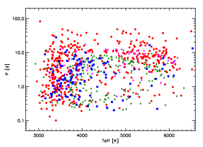
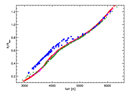
Figure 1.— Rotation period (left panel) and radius (right panel) vs. effective temperature for all sample stars. Blue squares: very young stars (up to 50 Myr); green triangles: young stars (between 85 and 150 Myr); magenta triangles: intermediate age stars (600–700 Myr); red circles: field stars.

Stars exhibit signs of magnetic activity through prominent emission of non-thermal radiation from coronal and chromospheric regions (Favata & Micela, 2003; Güdel, 2004; Hall, 2008), and through significant amounts of magnetic flux detectable on their surfaces (Donati & Landstreet, 2009; Reiners, 2012). It is believed that chromospheric and coronal regions are magnetically heated and that the generation of magnetic energy by large-scale dynamo action in the stellar convection zone is driven by rotation and convection (e.g., Charbonneau, 2010).

The relationship between stellar rotation and activity is extensively discussed in the literature. As soon as the first samples of activity measurements together with information on stellar rotation became available, it was realized that magnetic activity is stronger in rapid rotators, while slowly rotating stars (such as the Sun) exhibit relatively low levels of non-thermal emission and host only weak average magnetic fields. Pallavicini et al. (1981) found that the X-ray luminosity, $L_{\rm X}$, among cool stars (G–M) strongly depends on rotation rate, with $L_{\rm X}\propto(v_{\rm rot}\,\sin{i})^{1.9\pm 0.5}$ and no dependence on bolometric luminosity. The rich dataset from the Mt Wilson survey was used by Noyes et al. (1984) to study the relation between chromospheric activity and rotation. They showed that the ratio of chromospheric flux (observed in Caii) to bolometric flux correlates with the ratio of a color-dependent function $\tau(B-V)$, which they identified with the convective overturn time, to the rotation period, $P$. $\tau/P$ is proportional to the inverse Rossby number, 1/Ro (sometimes called Coriolis number), which describes the strength of the rotational effect on the convective flows. Under certain assumptions, the driving of a mean-field $\alpha\Omega$ dynamo is $\propto{\rm Ro}^{-2}$ (Durney & Latour, 1978; Montesinos et al., 2001), which motivates a scaling of activity in terms of the Rossby number.

It is clear that comparing $\tau/P$ against the ratio of chromospheric or coronal flux to bolometric flux (or luminosity) involves the possibility that bolometric flux and overturn time may actually depend on each other in such a way that they cancel each other, hence this comparison might only reflect the relation between non-thermal flux and rotation period alone, i.e., $L_{X}/L_{\rm bol}$ vs. $\tau/P$ simply reflects the relation $L_{X}$ vs. $1/P$. It was pointed out early on, e.g., by Basri et al. (1985) and Basri (1986) that in fact coronal emission and rotation provide a better correlation, or at least that it cannot be decided which one is the relevant relation.

The activity-rotation relationship was re-investigated by Pizzolato et al. (2003) on the basis of a large observational sample of 259 field and cluster stars with known X-ray emission and rotation rates. They showed that two emission regimes exist in cool stars: one for which X-ray luminosity depends on rotation period, and a second regime where the ratio between X-ray and bolometric luminosity is constant (called the saturated regime). They also derived an empirical overturn time, $\tau_{\rm e}$, to calculate an empirical Rossby number, ${\rm Ro}_{\rm e}=P/\tau_{\rm e}$, for their sample stars. The function $\tau_{\rm e}(B-V)$ was determined such that the scatter in the relation between normalized X-ray luminosity, $L_{\rm X}/L_{\rm bol}$, and ${\rm Ro}_{\rm e}$ is minimized for the non-saturated stars. Similar to Noyes et al. (1984) they found that $\tau_{\rm e}$ resembles theoretical overturn timescales. However, they also note that $\tau_{\rm e}$ roughly scales as $L_{\rm bol}^{-1/2}$, which implies that a relation $L_{\rm X}/L_{\rm bol}\propto{\rm Ro}_{\rm e}^{-2}$ is equivalent to $L_{\rm X}\propto P^{-2}$, without any dependence on other stellar parameters. Wright et al. (2011, W11) extended the available data and presented a sample of 824 cool stars with X-ray luminosities and rotation periods. Similar to Pizzolato et al. (2003), they determined an empirical overturn time by minimizing the scatter between normalized X-ray luminosity and a fit in terms of a power law in the (empirical) Rossby number. For the unsaturated stars in their sample, they found that $L_{\rm X}/L_{\rm bol}$ depends on Ro with an exponent of $-2.18\pm 0.16$ if all stars are used. The authors point out that the sample suffers from biases due to the selection of only X-ray detected sources, and they aim to overcome this bias by restricting the fit to an ‘unbiased’ subsample. From this sample, they found that the slope of the relation between $L_{\rm X}/L_{\rm bol}$ and Ro has an exponent of $-2.70\pm 0.13$.

A potential problem of empirically determined convective overturn times is that the physical meaning of this quantity is rather unclear since the overturn time varies with depth and it is not clear at which location the dynamo is most efficient. Furthermore, convective overturn times are likely to depend on other parameters like, e.g., metallicity, and change as stars age (e.g., Landin et al., 2010; Spada et al., 2013).

While it is obvious that one can always derive a function $\tau_{\rm e}$ that minimizes the scatter of the activity-rotation relation, it is not clear whether the similarity of the empirical overturn times with those resulting from mixing-length models of convection justifies conclusions concerning the nature of the dynamo process. In this paper, we therefore reduce the freedom of choosing this function by assuming that it is a power law of a fundamental stellar parameter that can, at least in principle, be determined independently for each sample star. For this we choose the stellar radius, $R$. Similarly, we assume a power law for the dependence of $L_{\rm X}/L_{\rm bol}$ on the rotational period, $P$. A fitting procedure based on minimizing scatter then yields optimal values for the two exponents of the power laws for the unsaturated part of the stellar sample. Our main result is that this procedure leads to a better fit of the data (less scatter) than the introduction of the empirical Rossby number. The resulting power-law exponents indicate that $L_{\rm X}\propto 1/P^{2}$ in the unsaturated regime. Since $L_{\rm X}$ is found to be directly related to the magnetic flux on the stellar surface (Pevtsov et al., 2003; Vidotto et al., 2014), this means that the generation of magnetic flux by the stellar dynamo in cool stars is a function only of rotation period, independent of other stellar parameters (such as radius or mass). Above a critical rotation period, $L_{\rm X}$ saturates at a level of $10^{-3}L_{\rm bol}$ for each star. Since our results are free from any assumption about the dynamo mechanism, they can be used to assess predictions from dynamo theory in the most general way.

2. Data

2.1. Stellar sample

We use the comprehensive sample analysed by W11. It is based on a compilation started by Pizzolato et al. (2003) and was extended by further literature data and from observations of stellar clusters. In total, the sample comprises 824 stars, of which we consider the 821 stars with masses below 1.4 M_⊙.

The sample contains stars of very different age, representing the evolution of stars from a few $10^{7}$ years up to ages of field stars. Specifically, the sample contains members of NGC 2547 (60 stars), IC 2602 (28), IC 2391 (13), $\alpha$ Persei (40), the Pleiades (146), NGC 2516 (14), Praesepe (20), the Hyades (49), as well as 445 field stars. More details on the references for individual measurements together with cluster ages and distances are provided in W11. Here, we adopt ages collected in that work. In our figures, we distinguish four groups of stellar ages, which we define as very young (up to 50 Myr; NGC 2547, IC 2602, IC 2391), young (between 85 and 150 Myr; $\alpha$ Persei, Pleiades, NGC 2516), intermediate (600–700 Myr; Praesepe and Hyades), and field stars.

2.2. Updated stellar parameters

2.2.1 Parameters derived from models

The catalog of W11 contains measured data for rotation, X-ray luminosity, and color, together with several other indicators. In addition, stellar parameters such as mass, effective temperature, radius, and depth of the convective envelope were calculated from the models of Siess et al. (2000). We updated these parameters by interpolating the tables from Siess et al. (2000), which led in some cases to values that somewhat differ from those given in W11. The discrepancy is most pronounced for the depth of the convective envelope. This is probably due to the fact that the parameter range is poorly covered for masses around $M=0.35$ M_⊙ in the tables of Siess et al. (2000). The minimum mass for the appearance of a radiative core is $M=0.35$ M_⊙ (Chabrier & Baraffe, 1997), and we set the stars to be fully convective for $M\leq 0.35$ M_⊙, thus extending the tabulated points in Siess et al. (2000). For consistency, we also updated the stellar parameters mass, radius, effective temperature, and we redetermined bolometric luminosity and used these values for our analysis.

2.2.2 Rotation periods

For some of the stars in the sample, improved measurements of rotation periods became available during the last years, and some of them significantly differ from the ones collected in W11. The new periods used for the analysis in this paper are listed in Table 1.

Figure 1 shows an overview of the sample. We plot rotation period (left) and radius (normalized by the solar radius; right) versus effective temparature for all sample stars, indicating ages by different colors and symbols. The sample shows the typical signatures evident of mass-dependent rotational evolution (see, e.g., Barnes & Kim, 2010; Reiners & Mohanty, 2012).

We note that none of the results shown in the following changes qualitatively if the original stellar parameters and periods from W11 are adopted.

Table 1Updated rotation periods

Star	Period [d]		Reference
	Old	Updated
GJ 182	1.86	4.41	(ks07)
GJ 494	1.54	2.889	(ks07)
GJ 551	42.00	82.53	(ks07)
GJ 2123A	7.79	0.32	(ks07)
GJ 669A	19.81	0.95	(ks07)
HD 95650/GJ410	2.94	14.81	(fh00)
GJ 388/AD Leo	2.6	2.23	(en09)
G99-49	0.5	1.81	(ir11)
GJ 1156	0.87	0.491	(ir11)
GJ 493.1	0.21	0.6	(ir11)
GJ 791.2	0.32	0.346	(ir11)

References – (ks07): Kiraga & Stepien (2007); (fh00): Fekel & Henry (2000); (ir11): Irwin et al. (2011); (en09): Engle et al. (2009)

3. Results

3.1. The generalized rotation-activity relation

We assume that the normalized X-ray luminosity, $L_{\rm X}/L_{\rm bol}$, depends on rotation period and on a combination of parameters given by the structure of the star, such as mass, radius, temperature, or depth of the convection zone. Because they all scale in some way with the mass or the radius of the star, we condense the dependence on stellar parameters in the radius $R$, and search for an optimal representation that minimizes the scatter in $L_{\rm X}/L_{\rm bol}$. For a generalized dependence of $L_{\rm X}/L_{\rm bol}$ on $P$ and $R$ in the form of a combination of power laws,

$$\frac{L_{\rm X}}{L_{\rm bol}}\propto R^{\alpha}P^{\beta},$$ (1)

we considered fits through the resulting distributions of points in the plane $\log(L_{\rm X}/L_{\rm bol})$ vs. $\log(kR^{\alpha}P^{\beta})$, where $k$ represents the constant of proportionality in Eq. 1. The fit curves are composed of two linear parts: one for the unsaturated regime, which should follow the relationship given by Eq. 1 and therefore must have a slope of unity, and another linear fit for the saturated part of the sample. The best fit is then defined as the one showing the minimum scatter of the data points with respect to the fit curve. The location of the break in the slope of the fit curve between the unsaturated and the saturated parts is found by including the break point in the minimization process.

The linear regression curves are calculated using an adapted version of a procedure studied by Isobe et al. (1990), who provide algorithms for five methods for linear regression fits to bivariate data. The different methods are useful for taking into account different distributions of uncertainties in the data. The ‘standard’ way of fitting a slope in a variable Y to another variable X is the ordinary least squares method, OLS(Y$|$X). This method assumes that Y measures (with uncertainty) the value of a parameter that depends on a known variable X (with no or very little uncertainty). A second method, OLS(X$|$Y), calculates the fit under the assumption that Y is the variable that is well defined and the scatter in the observed sample is due to a distribution (or measurement uncertainties) in X. A third method, the OLS bisector, performs the fit under the assumption that the scatter in the distribution is due to scatter in both variables X and Y with symmetrically distributed scatter. This relation provides the regression that produces the ’best-looking’ fit, i.e., a line that lies closest to all data points. In our situation, typical uncertainties in the variables X and Y are not symmetric. The intrinsic scatter in $L_{\rm X}$ of a sun-like star due to stellar variability is typically on the order of a factor of 2 but higher during flare events (Schmitt et al., 1995). Uncertainties in $L_{\rm bol}$ and differences between X-ray calibrations from different instruments can add more uncertainty so that a factor of two is probably a lower limit for the uncertainty in $L_{\rm X}/L_{\rm bol}$ in our sample. Stellar radii are derived in a consistent way, so that residual errors are probably only a few percent. The rotation periods in the sample are also relatively well constrained. We do not expect any systematic differences between periods measured by different authors, and the variability of observed rotation periods in sun-like stars is reported to be on the order of 10–20 % or lower (Donahue et al., 1996), i.e., the uncertainty in our variable X is a factor of 10–20 less than the uncertainty in our variable Y. Thus, we conclude that OLS(Y$|$X) is the appropriate method for the calculation in our case. We thereby ignore the uncertainty in $P$, which probably leads to a slight underestimate of the slope (Isobe et al., 1990). We estimate this effect to be less than 0.1 from tests using the OLS(Y$|$X) and OLS bisector methods.

For the optimal solution with a scatter of 0.346 dex we find values of $\alpha=-4.3$, $\beta=-2.2$, $k=1.86\times 10^{-3}\,$d^-β R${}_{\odot}^{-\alpha}$, and the break point at $\log(L_{\rm X}/L_{\rm bol})=\log(kR^{\alpha}P^{\beta})=-3.14$. Up to 3 digits, the scatter is the same also for the combination $\alpha=-4$ and $\beta=-2$. For simplicity, we shall consider these values as our optimal solution in what follows.

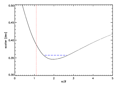
Figure 2.— Scatter (1 $\sigma$) of $L_{\rm X}/L_{\rm bol}$ around Eq. 1 for different values of the ratio $\alpha/\beta$. The blue dashed line marks the 2$\sigma$-interval for $\alpha/\beta$ assuming that the statistical uncertainty in the measurement of $L_{\rm X}/L_{\rm bol}$ equals the minimum scatter 0.346 dex. The red dotted line shows the approximate location derived in W11 from the Rossby-formulation based on their ’unbiased’ subsample of stars (see text).

In order to determine a confidence interval for the optimal solution, we note that the nature of the assumed power-law relationship in the unsaturated part implies that the scatter of the data points around Eq. 1 on the log-log plane, and hence the quality of the fit, depends only on the ratio of the exponents, $\alpha/\beta$. We thus calculated the scatter as a function of $\alpha/\beta$ by determining the standard deviation of the data points from the broken power-law fit, using the value of the break point that minimizes the standard deviation for each given value of $\alpha/\beta$. We carried out this procedure for 101 values for each of the parameters $\alpha$ and $\beta$ with $-6\leq\alpha\leq 0$ and $-6\leq\beta\leq 0$. The resulting relation between the scatter (in dex) and $\alpha/\beta$ is shown in Fig. 2. We find a smooth distribution with a minimum located at $\alpha/\beta=1.93$ (2.06 for the original sample). We estimate a confidence interval of this solution assuming that the uncertainties in $L_{\rm X}/L_{\rm bol}$ follow a normal distribution around our fit. In other words, we assume that the uncertainty of each individual measurement is equal to the minimum of the scatter. With a minimum scatter of 0.346 dex and a total number of 349 measurements of stars in the unsaturated regime, we estimate (see Press et al., 1986) as 2$\sigma$ confidence interval of the ratio $\alpha/\beta$ the range

$$1.53<\frac{\alpha}{\beta}<2.66,$$ (2)

which is indicated by the blue dashed line in Fig 2. For the individual values of $\alpha$ and $\beta$ we find the $2\sigma$ intervals

$$-5.04< \alpha <-3.54,$$ (3)

$$-2.37< \beta <-1.88.$$ (4)

We note that the assumption of normally distributed uncertainties in the individual measurements of $L_{\rm X}/L_{\rm bol}$ is probably not entirely correct. Nevertheless, a 1 $\sigma$ uncertainty of 0.346 dex (more than a factor of 2) appears to be a realistic estimate that captures several systematic effects, such as instrument differences, flares (occuring statistically), and contamination from binaries. Ratios outside the confidence interval can therefore be regarded as statistically unlikely, even if we do not fully understand the sources of the measurement uncertainties. The dotted red vertical line in Fig. 2 indicates the value of $\alpha/\beta=1.1$ that we infer for the formulation of W11 in terms of the Rossby number (see Sect. 3.2 below); it is clearly outside the 2$\sigma$ confidence interval.

Our result provides information on the dependence between the parameters used in Eq. 1. It is important to realize that in the available sample, rotation, color, mass, radius, age, etc. are severely degenerate, for example because very few sun-like stars are rapidly rotating. Our result is that rotation period, $P$, and radius, $R$ can explain the existing activity observations but underlying physical relations may be hidden by sample degeneracies. Further data on stars occupying sparsely populated parameter ranges would help to remove this degeneracy.

3.2. Comparison to Wright et al. (2011)

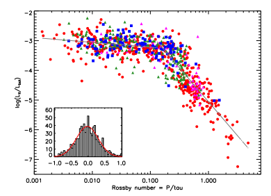
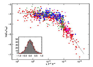
Figure 3.— Normalized X-ray luminosity as a function of empirical Rossby number (left) and as a function of $kP^{2}R^{4}$ (right). Different colored symbols show stars at different ages (see Fig. 1). The distributions are fit using a broken power-law (grey lines) with the break at ${\rm Ro}=0.13$ (left panel) and $\log{kP^{-2}R^{-4}}=-3.14$ (right panel). Scatter around the fit is shown in the inset of each panel, a Gauss fit is overplotted in each panel’s inset as a red line.

Table 2Slope $\gamma$ in the unsaturated regime for the three cases in W11

Sample	OLS(Y$|$X)	OLS bisector	OLS(X$|$Y)
$0.13<$ Ro	$-2.16\pm 0.08$	$-2.58\pm 0.08$	$-3.17\pm 0.12$
$0.2<$ Ro $<3.0$	$-2.36\pm 0.09$	$-2.90\pm 0.09$	$-3.71\pm 0.17$
‘unbiased’ sample∗	$-1.91\pm 0.18$	$-2.24\pm 0.16$	$-2.67\pm 0.25$

^∗ valid in the range $0.3<$ Ro $<3$; HD 81809 is not in the catalog

Wright et al. used the same sample of stars to obtain a power-law relation between $L_{\rm X}/L_{\rm bol}$ and an empirical Rossby number by considering the convective overturn time, $\tau$, as an adjustable function of stellar mass. By minimizing the scatter of the data points with respect to the power-law fit they determined the slope $\gamma$ in

$$\frac{L_{\rm X}}{L_{\rm bol}}\propto\left(\frac{P}{\tau}\right)^{\gamma}$$ (5)

in the unsaturated regime. Including all 824 stars in their sample, they report $\gamma=-2.18\pm 0.16$ for the best fitting slope. The authors argue that an OLS bisector fit is appropriate for this sample. We question this choice because of the asymmetric distribution of the uncertainties (see Section 3). To compare the results from different fit methods, we re-calculated the slope using three different methods, OLS(Y$|$X), OLS bisector, and OLS(X$|$Y). The results are shown in Table 2. We include three subsamples that are mentioned in W11, the full sample (with Ro $>0.13$), a sample with Ro $>0.2$, and their ’unbiased’ sample (see below). We observe rather large inconsistencies between our results and their findings, which may be partly because we cannot reconstruct the overturn times W11 used for their fit. These overturn times follow the relation from Pizzolato et al. (2003) but W11 convert $V-K$ into $B-V$ based on a relation that is not provided for all stars. We therefore used the convective overturn times as determined in W11 as a function of mass, which do not significantly differ from those of Pizzolato et al. as shown in W11.

An important point in the results from W11 is their construction of an ‘unbiased’ sample. The authors argue that X-ray bright sources are easier to detect and may therefore be overrepresented with respect to stars that are X-ray dim. This could be particularly important for the mean $L_{X}$ for a given value of $P$ because slow rotators with low X-ray brightness may be systematically underrepresented. To construct an X-ray complete sample, they chose the 36 stars from Donahue et al. (1996) for which rotation periods could be measured over five or more seasons. According to W11, the 36 stars all show measurable X-ray emission and W11 argue that the sample therefore does not suffer from X-ray luminosity bias. We do not agree that this particular sample should be less biased than others, in particular because it is a sample of 36 selected out of 100 stars based on detectability of photometric periods. We calculated the slope for this sample and include our results in Table 2. We cannot reproduce the value of $\gamma=-2.7$ for the OLS bisector method. We revisit the question of luminosity bias in Section 3.6.

For completeness, we compare the scaling reported in W11 ($\gamma=-2.7$) to our solution. We note that this is not comparing the same samples, but we find it helpful to discuss the $\gamma=-2.7$ scaling to our generalized results. The convective overturn time for the W11 solution was parametrized in terms of stellar mass, $M$, by a second-order double-logarithmic polynomial (see their Eq. 11). For the stars considered in the unsaturated part of the sample, the values of $M/M_{\odot}$ and $R/R_{\odot}$ are almost identical, so that we can replace $M/M_{\odot}$ in their relation by $R/R_{\odot}$ without introducing significant scatter. Furthermore, we can approximate their Eq. (11) by the first-order relation

$$\log{\tau}=1.19-1.08\log{M/M_{\odot}},$$ (6)

so that we can rewrite Eq. (5) in the form

$$\frac{L_{\rm X}}{L_{\rm bol}}\propto\left(\frac{R^{-1.08}}{P}\right)^{2.7}=P^{-2.7}R^{-2.9},$$ (7)

which is equivalent to Eq. (1) with $\alpha/\beta=2.9/2.7=1.1$. This value is indicated by red dotted line in Fig. 2; it is outside the 2$\sigma$ confidence interval for the optimal value of $\alpha/\beta$. The expected scatter for $\alpha/\beta=1.1$ is approximately 0.38 dex. A more direct comparison of the fit qualities can be achieved if we use the original Rossby scaling provided by W11 and compare its scatter to the one determined from the distribution using $\alpha=-4$ and $\beta=-2$. In Fig. 3, we show normalized X-ray luminosity as a function of Rossby number (left panel) and as a function of $kP^{-2}R^{-4}$ for minimal scatter (right panel). In both panels, we overplot broken power-law fits to the data. For the values from W11, we break the power law at ${\rm Ro}_{\rm sat}=0.13$ as reported in that work. For the values of $k$ and the power law break in the $\alpha=-4$ and $\beta=-2$ solution we take the values of the optimal solution.

From both descriptions, we determined the scatter around the power-law fit by calculating the standard deviations of the distributions shown in the insets of the panels of Fig. 3. For the Rossby formulation, the standard deviation is $\sigma=0.371$ dex while for the generalized formulation (right panel in Fig. 3) we have $\sigma=0.346$ dex (as found in Sect.3.1). Compared to the simplified approach using Eq. (6), the value for the optimized Rossby formulation is closer to, but still considerably higher than, the minimum from our generalized formulation.

3.3. Comparison to Pizzolato et al. (2003)

A quadratic dependence of X-ray luminosity on rotation rate alone was already suggested by Pallavicini et al. (1981). More recently, Pizzolato et al. (2003) pointed out that the empirical turnover time approximately scales as $\tau\propto L_{\rm bol}^{-1/2}$. With a rotation-activity relation of the form $L_{\rm X}/L_{\rm bol}\propto{\rm Ro}^{-2}$ they then obtain

$$\frac{L_{\rm X}}{L_{\rm bol}}\propto{\rm Ro}^{-2}\propto\frac{1}{P^{2}L_{\rm bol}},$$ (8)

which is equivalent to $L_{\rm X}\propto P^{-2}$ . This relation is consistent with the result of our generalized approach, which can be seen as follows. Since $L_{\rm bol}\propto R^{2}T_{\rm eff}^{4}$, and also for the non-saturated stars approximately $T_{\rm eff}\propto R^{1/2}$, we find with $\alpha=-4$ and $\beta=-2$ the relation

$$\frac{L_{\rm X}}{L_{\rm bol}}\propto P^{-2}R^{-4}\propto\frac{1}{P^{2}(R^{2}T^{4})}\propto\frac{1}{P^{2}L_{\rm bol}},$$ (9)

which is identical to the relation in Eq. (8). The factor of $R^{-4}$ effectively compensates the normalization by the bolometric luminosity, indicating that the normalization is in fact unwarranted in the unsaturated regime.

Since we have the values of $L_{\rm bol}$ for the stars in our sample, we can also directly consider the relation $L_{\rm X}/L_{\rm bol}\propto 1/(P^{2}L_{\rm bol})$. It turns out that the scatter from this relation is 0.340 dex, which is even slightly lower than the minimum scatter of 0.346 dex for the relation given in Eq. 1. This supports the conclusion that the relation between $L_{\rm X}$ and $P^{-2}$ is better constrained than the relation between $L_{\rm X}/L_{\rm bol}$ and some combination of $P$ and other stellar parameters.

3.4. Saturation

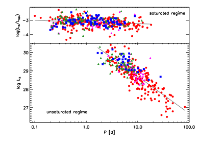
Figure 4.— Separate representations of X-ray activity vs. rotation period in the unsaturated (lower part) and saturated (upper part) regimes. Activity is represented in terms of $L_{\rm X}$ in the unsaturated regime and in terms of $L_{\rm X}/L_{\rm bol}$ in the saturated regime.

We have seen that the total X-ray luminosity in the unsaturated regime scales with $P^{-2}$ and does not depend on any other stellar parameter. When the total X-ray luminosity reaches a critical value of about $10^{-3}L_{\rm bol}$, it does not grow further for shorter rotational periods, i.e., activity saturates. The critical period at which saturation sets in therefore depends on the stellar luminosity, $L_{\rm bol}$. We can use our optimal solution to determine the value of the critical period. For $\alpha=-4$, $\beta=-2$, and $k=1.86\times 10^{-3}$ d² R${}_{\odot}^{4}$, saturation sets in at about $\log{kP^{-2}R^{-4}}=-3.14$. With $L_{\rm bol}\propto R^{4}$ and $L_{\odot}=3.853\cdot 10^{33}\,$erg s^-1 we find

$$P_{\rm sat}\,{\rm[d]}=1.6\left(\frac{L_{\rm bol}}{L_{\odot}}\right)^{-1/2}=\left(\frac{L_{\rm bol}}{1.1\cdot 10^{34}}\right)^{-1/2}$$ (10)

where $L_{\rm bol}$ is in units of erg s^-1. This result is similar to Eq. (6) of Pizzolato et al. (2003).

For this value of the critical period, we show the distribution of $\log L_{\rm X}$ vs. $P$ for the unsaturated regime together with $\log(L_{\rm X}/L_{\rm bol})$ vs. $P$ for the saturated regime in the lower and upper panels of Fig. 4, respectively. For the unsaturated regime, we find the relation

$$\log{L_{\rm X}}=(30.71\pm 0.05)-(2.01\pm 0.05)\log{P},$$ (11)

which is consistent with our optimal value $\beta=-2$.

3.5. A slope in the saturated regime

All three representations shown in Figs. 3 and 4 indicate a slight slope of the rotation-activity relationship in the saturated regime, i.e. some remnant dependence of the activity on rotation (or other parameters) even for very rapidly rotating stars. Quantitatively, we find for the different representations:

$$\log{\frac{L_{\rm X}}{L_{\rm bol}}} = (-3.37\pm 0.06)-(0.16\pm 0.03)\log{\rm Ro},$$

$$\log{\frac{L_{\rm X}}{L_{\rm bol}}} = (-3.04\pm 0.02)-(0.07\pm 0.01)\log{(kP^{2}R^{4})},$$

$$\log{\frac{L_{\rm X}}{L_{\rm bol}}} = (-3.12\pm 0.01)-(0.11\pm 0.03)\log{P}.$$

There is a statistically significant slope in all three cases. The slope is least significant (but still above $3\sigma$) in the parameterization with $P$, while at $\geq 5\sigma$ and more in the two other cases. The slope is likely due to a remaining dependence of the dynamo on rotation period even when saturation is reached, but it may also be influenced by small differences in the saturation level between stars of different mass.

3.6. Luminosity bias

Figure 5.— Slope $\beta$ for subsamples that contain stars out to a maximum distance. Error bars show 1$\sigma$ uncertainties.

W11 pointed out that the slope of the rotation-activity relation may suffer from a luminosity bias. A possible consequence is that the least X-ray bright stars are systematically missed, so that the average X-ray luminosity among the least active stars (the slowest rotators) is overestimated. This would lead to a slope shallower than the true relation. We are lacking a statistically unbiased, complete sample of stars with X-ray and rotation period measurements. Nevertheless, the large sample of targets allows us to test whether the slope $\beta$ that we derive in the unsaturated regime depends on the distance to the stars in the sample. A luminosity bias would be less pronounced in a sample of nearby stars and become more important if we include increasingly distant objects. We carried out this test computing the slope $\beta$ for stars in the sample with distances out to 15, 30, 60, 120, 240, and 480 pc. The results are shown in Fig. 5. We find no significant trend of $\beta$ as a function of distance limit. There is a marginal trend towards higher absolute values of the slope at large distances, but it is dominated by the sample limited to 15 pc, which has large uncertainties. We conclude that our results do not show evidence of a luminosity bias.

4. Discussion

The result of our generalized analysis of the rotation-activity relation can be summarized as follows: The total X-ray luminosity scales with rotation period ($P^{-2}$) as long as stellar activity is not saturated, and X-ray activity saturates for a given star when $L_{\rm X}/L_{\rm bol}$ reaches a level of about $10^{-3}$. In the unsaturated regime, this description is equivalent to a scaling $L_{\rm X}/L_{\rm bol}\propto P^{-2}R^{-4}$, which could be written as a Rossby number scaling of the form $L_{\rm X}/L_{\rm bol}\propto{\rm Ro}^{-2}$ if the convective overturn time scales as $\tau\propto R^{-2}\propto L_{\rm bol}^{-1/2}$. Furthermore, for a given star in the saturated regime, $L_{\rm X}/L_{\rm bol}$ still shows a weak but significant dependence on rotation. In what follows we discuss some physical implications of these results.

4.1. $L_{\rm X}\propto P^{-2}$

This relationship means that two stars with the same rotation period emit the same X-ray luminosity, irrespective of their mass or radius. Since observations indicate that $L_{\rm X}$ is proportional to $\Phi_{\rm s}$, the total magnetic flux at the stellar surface (Pevtsov et al., 2003), it implies that $\Phi_{\rm s}$ depends only on the rotation rate, but not on any other stellar parameter. This is consistent with a recent study by Vidotto et al. (2014) on the relationship between the large-scale surface magnetic flux determined by Zeeman Doppler Imaging, $\Phi_{\rm V}$, and X-ray luminosity: the two relations, $L_{\rm X}$ vs. $\Phi_{\rm V}$ and $L_{\rm X}/L_{\rm bol}$ vs. $\Phi_{\rm V}$, yield nearly the same power-law exponents (1.80 and 1.82, respectively). This means that $\Phi_{\rm V}$ is uncorrelated with $L_{\rm bol}$ and, therefore, uncorrelated with stellar radius or mass. Similarly, the scalings with rotation period of $\Phi_{\rm V}$ and magnetic flux density ($\Phi_{\rm V}$ divided by surface area) show the same power-law exponent, which means that the rotation rate is uncorrelated with radius or mass (consistent with our value $\alpha=-4$).

The absence of a dependence of $L_{\rm X}$ on stellar parameters apart from rotation means that a bigger star shows the same magnetic surface flux as a smaller star at the same rotation rate. One would have naively expected that the bigger volume of the convection zone available for dynamo action would also lead to more magnetic flux being produced by the dynamo, so that also more flux emerges at the surface. Also, bigger scales could imply less dissipation of the large-scale field by turbulent diffusion, thus effectively increasing the net driving of the dynamo. On the other hand, the turbulent magnetic diffusivity probably decreases towards cooler (smaller) stars since the convective motions are slower; the net effect on dynamo driving is unclear.

4.2. Saturation

The existence of a limiting value $L_{\rm X}/L_{\rm bol}\approx 10^{-3}$ for very fast rotators lends itself to at least three possible interpretations.

Firstly, it can be seen as indicating that there is a maximum fraction of the total energy flux of the star that can be converted into X-ray flux. This could be related to an upper limit of the efficiency of converting the energy flux into magnetic energy (e.g., Reiners et al., 2009; Christensen et al., 2009), although the relation between X-ray flux and magnetic energy generation in the convection zone is unclear.

A second possible interpretation can be inferred from the scaling of the critical rotation period for saturation given in Eq. (10): $P_{\rm sat}\propto L_{\rm bol}^{-1/2}\propto R^{-2}$. This relation implies that the critical rotation rate, $2\pi/P_{\rm sat}$, is proportional to the surface area of the star, so that it can be interpreted as the rotation rate at which the magnetic surface flux in bipolar regions fills the complete stellar surface (e.g., Vilhu, 1984). If the X-ray flux ultimately results from the interaction of surface magnetic flux with near-surface flows, saturation could be a result of this situation. In this picture, the filling of the surface would also need to imply that the total surface magnetic flux is saturated, for which evidence is reported in Reiners et al. (2009). For a solar-type star, saturation occurs at $L_{\rm X}\approx 4\cdot 10^{30}\,$erg s^-1, roughly a factor of $10^{3}$ above the value at activity maxima of the Sun today, during which the area fraction of active regions is a few percent. For $L_{\rm X}\propto\Phi_{\rm{}_{s}}$ (Pevtsov et al., 2003), the saturated X-ray luminosity would not be reached for a Sun fully covered by active regions (e.g., Vaiana & Rosner, 1978; Drake et al., 2000); however, it would be consistent for a steeper relationship, such as $L_{\rm X}\propto\Phi_{\rm{}_{s}}^{1.8}$ proposed by Vidotto et al. (2014).

Another interpretation can be given in terms of the nonlinearities that determine the amplitude of the dynamo-generated magnetic field (R.H. Cameron, private communication). The present Sun is located in the lower part of the unsaturated regime and its differential rotation is almost invariant during the activity cycle. This means that the magnetic energy is small compared to the kinetic energy in the differential rotation, which therefore does not experience a strong back reaction of the toroidal magnetic field it generates. The field amplitude in the unsaturated regime is thus determined by a nonlinearity affecting the generation of the poloidal field (‘$\alpha$ quenching’). As the rotation rate grows along the unsaturated branch, at some stage the magnetic energy becomes comparable to the kinetic energy of differential rotation, so that a strong back reaction occurs (‘$\Omega$ quenching’). If the corresponding nonlinearity is sufficiently hard, it results in a quasi-saturated regime that is (almost) independent of the rotation rate.

4.3. Dynamo models

Given the present state of our understanding of solar and stellar dynamos (see, e.g., Charbonneau, 2010), drawing a quantitative connection between the dynamo mechanism and the observed activity indices is by no means straightforward. It seems uncontroversial that the toroidal flux is generated (from poloidal flux) by differential rotation (the $\Omega$-effect) while the poloidal flux is regenerated by some kind of $\alpha$-effect. The latter could be due to the action of cyclonic convection on the toroidal field, i.e., the classical Parker loop, which would bring the Rossby number into consideration. However, it could also result from the Babcock-Leighton mechanism, i.e., the systematic tilt of bipolar regions with respect to the direction of rotation. This tilt can result from the action of the Coriolis force on flows along rising flux tubes (Fan, 2009). These flows are not of a convective nature and thus independent from a Rossby number.

The combination of $\alpha$-effect and $\Omega$-effect provides the driving of the dynamo, but the relation of this driving to rotation is uncertain. Since the $\alpha$-effect is due to the action of the Coriolis force, one can argue that it should be proportional to the rotation rate, at least for not too rapid rotation. The relation of differential rotation to the overall rotation rate is much more unclear, so that the scaling of dynamo driving (expressed by a non-dimensional dynamo number involving the product of $\alpha$- and $\Omega$-effect) with rotation is rather uncertain. The dependence on other stellar parameters is unclear as well and mostly addressed by crude dimensional arguments.

The scaling of the amplitude of the dynamo-generated field with the driving dynamo number depends crucially on the kind of nonlinear backreaction of the magnetic field on its sources, which limits the growth of the magnetic energy. There are various nonlinearities that could play a role here, e.g., quenching of $\alpha$-effect and differential rotation, flux loss by magnetic buoyancy, driving of large-scale flows, all of which are not well understood quantitatively. As a consequence, dynamo models mostly consider them in an ad-hoc fashion. Keeping in mind these severe uncertainties, it is interesting to note that at least some models show roughly similar dependencies of the field amplitude on the dynamo driving (dynamo number, $N_{\rm D}$): $\propto N_{\rm D}^{1/2}$ for simple one-dimensional models (Stix, 1972; Schmitt & Schüssler, 1989), and $\propto N_{\rm D}^{0.65}$ for a state-of-the-art 2D flux-transport dynamo model (Karak et al., 2014); the latter is also consistent with the result from an earlier model by Jouve et al. (2010). However, quite different dependencies are found with other models (e.g., Robinson & Durney, 1982) and a dynamo model with $\alpha$-effect and differential rotation taken from global 3D simulations even fails to show an increase of activity with rotation rate (Dubé & Charbonneau, 2013).

Eventually, the observed activity indices (such as $L_{\rm X}$) are related to the surface flux emerging in bipolar magnetic regions. How this flux is connected quantitatively with the general dynamo amplitude, i.e., the amount of magnetic flux or magnetic energy generated in the convection zone, depends on the detailed processes leading to flux emergence. Again, these processes are not well understood and different mechanisms are possible: instability of strong magnetic flux tubes (Fan, 2009) or buoyant local flux concentrations compressed to super-equipartion by turbulent convective flows (Nelson et al., 2011, 2014).

5. Concluding remarks

We used activity and rotation measurements of 821 stars, compiled in the sample of W11, to perform a generalized analysis of the rotation-activity relation. The sample was updated with recent period measurements from the literature. We considered the relation of normalized X-ray luminosity, ${L_{\rm X}/L_{\rm bol}}$, on rotation period, $P$, and stellar parameters condensed in the radius, $R$, in the functional form $R^{\alpha}P^{\beta}$. In the unsaturated regime, we found the representation with the least scatter for $\alpha=-4$ and $\beta=-2$. Since approximately $L_{\rm bol}\propto R^{4}$, this solution is equivalent to $L_{\rm X}\propto P^{-2}$, a relation that had already been found by Pallavicini et al. (1981) and Pizzolato et al. (2003). On the other hand, the most recent parametrization of the activity-rotation relation in terms of the Rossby number by W11 does show a significantly higher scatter.

In the subsample of stars that are in the saturated regime, we found a slight but significant growth of ${L_{\rm X}/L_{\rm bol}}$ with faster rotation. It is unclear whether this trend is due to an effect of $P$ beyond the saturation limit or results from a degeneracy between stellar mass and rotation rate reflecting that $L_{\rm X}/L_{\rm bol}$ is slightly larger for more luminous stars.

Formally, we can rewrite $R^{-4}P^{-2}$ in terms of a Rossby number, ${\rm Ro}=P/\tau$, if the convective overturn time scales as $\tau\propto R^{-2}\propto L_{\rm bol}^{-1/2}$. We then obtain ${L_{\rm X}/L_{\rm bol}}\propto{\rm Ro}^{-2}$. Unless we have a reliable determination of the Rossby number in stellar convection zones (provided that this is possible at all), we cannot decide whether the physical mechanism behind the rotation-activity relation is better represented by a Rossby-number scaling of ${L_{\rm X}/L_{\rm bol}}$ or by a purely rotational scaling of $L_{\rm X}$ independent of other stellar parameters. However, since the latter involves no assumptions on physical conditions to be valid in the star, we favour this description and find it unnecessary to explain the rotation-activity relation in terms of the Rossby formulation.

The dependence of dynamo driving (as possibly expressed by a dynamo number), its nonlinearity, and the amount of magnetic flux emerging at the stellar surface on rotation and other stellar parameters (such as radius) is quite unclear. The various factors may well combine to a result that makes the surface flux independent of stellar radius as indicated by our analysis. One possible form to condense this independence into a physical model is to assume a Rossby scaling with a convective overturn time that is (exactly) proportional to the square-root of the stellar luminosity. One can think of many other families of models that can potentially lead to this result, and this opens room for more general descriptions of the magnetic dynamo.

References

- Barnes & Kim (2010) Barnes, S. A., & Kim, Y.-C. 2010, ApJ, 721, 675
- Basri (1986) Basri, G. 1986, in Lecture Notes in Physics, Berlin Springer Verlag, Vol. 254, Cool Stars, Stellar Systems and the Sun, ed. M. Zeilik & D. M. Gibson, 184
- Basri et al. (1985) Basri, G., Laurent, R., & Walter, F. M. 1985, ApJ, 298, 761
- Catalano & Marilli (1983) Catalano, S., & Marilli, E. 1983, A&A, 121, 190
- Chabrier & Baraffe (1997) Chabrier, G., & Baraffe, I. 1997, A&A, 327, 1039
- Charbonneau (2010) Charbonneau, P. 2010, Living Reviews in Solar Physics, 7, 3
- Christensen et al. (2009) Christensen, U. R., Holzwarth, V., & Reiners, A. 2009, Nature, 457, 167
- Donahue et al. (1996) Donahue, R. A., Saar, S. H., & Baliunas, S. L. 1996, ApJ, 466, 384
- Donati & Landstreet (2009) Donati, J.-F., & Landstreet, J. D. 2009, ARA&A, 47, 333
- Drake et al. (2000) Drake, J. J., Peres, G., Orlando, S., Laming, J. M., & Maggio, A. 2000, ApJ, 545, 1074
- Dubé & Charbonneau (2013) Dubé, C., & Charbonneau, P. 2013, ApJ, 775, 69
- Durney & Latour (1978) Durney, B. R., & Latour, J. 1978, Geophysical and Astrophysical Fluid Dynamics, 9, 241
- Engle et al. (2009) Engle, S. G., Guinan, E. F., & Mizusawa, T. 2009, in American Institute of Physics Conference Series, Vol. 1135, American Institute of Physics Conference Series, ed. M. E. van Steenberg, G. Sonneborn, H. W. Moos, & W. P. Blair, 221–224
- Fan (2009) Fan, Y. 2009, Living Reviews in Solar Physics, 6, 4, http://www.livingreviews.org/lrsp-2009-4
- Favata & Micela (2003) Favata, F., & Micela, G. 2003, Space Sci. Rev., 108, 577
- Fekel & Henry (2000) Fekel, F. C., & Henry, G. W. 2000, AJ, 120, 3265
- Güdel (2004) Güdel, M. 2004, A&A Rev., 12, 71
- Hall (2008) Hall, J. C. 2008, Living Reviews in Solar Physics, 5, 2
- Irwin et al. (2011) Irwin, J., Berta, Z. K., Burke, C. J., et al. 2011, ApJ, 727, 56
- Isobe et al. (1990) Isobe, T., Feigelson, E. D., Akritas, M. G., & Babu, G. J. 1990, ApJ, 364, 104
- Jouve et al. (2010) Jouve, L., Brown, B. P., & Brun, A. S. 2010, A&A, 509, A32
- Karak et al. (2014) Karak, B. B., Kitchatinov, L. L., & Choudhuri, A. R. 2014, ArXiv e-prints
- Kiraga & Stepien (2007) Kiraga, M., & Stepien, K. 2007, Acta Astron., 57, 149
- Landin et al. (2010) Landin, N. R., Mendes, L. T. S., & Vaz, L. P. R. 2010, A&A, 510, A46
- Liefke & Schmitt (2005) Liefke, C., & Schmitt, J. H. M. M. 2005, in ESA Special Publication, Vol. 560, 13th Cambridge Workshop on Cool Stars, Stellar Systems and the Sun, ed. F. Favata, G. A. J. Hussain, & B. Battrick, 755
- Middelkoop (1982) Middelkoop, F. 1982, A&A, 107, 31
- Montesinos et al. (2001) Montesinos, B., Thomas, J. H., Ventura, P., & Mazzitelli, I. 2001, MNRAS, 326, 877
- Nelson et al. (2011) Nelson, N. J., Brown, B. P., Brun, A. S., Miesch, M. S., & Toomre, J. 2011, ApJ, 739, L38
- Nelson et al. (2014) Nelson, N. J., Brown, B. P., Sacha Brun, A., Miesch, M. S., & Toomre, J. 2014, Sol. Phys., 289, 441
- Noyes et al. (1984) Noyes, R. W., Hartmann, L. W., Baliunas, S. L., Duncan, D. K., & Vaughan, A. H. 1984, ApJ, 279, 763
- Pallavicini et al. (1981) Pallavicini, R., Golub, L., Rosner, R., et al. 1981, ApJ, 248, 279
- Pevtsov et al. (2003) Pevtsov, A. A., Fisher, G. H., Acton, L. W., et al. 2003, ApJ, 598, 1387
- Pizzolato et al. (2003) Pizzolato, N., Maggio, A., Micela, G., Sciortino, S., & Ventura, P. 2003, A&A, 397, 147
- Press et al. (1986) Press, W. H., Flannery, B. P., & Teukolsky, S. A. 1986, Numerical recipes. The art of scientific computing
- Reiners (2012) Reiners, A. 2012, Living Reviews in Solar Physics, 9, 1
- Reiners et al. (2009) Reiners, A., Basri, G., & Browning, M. 2009, ApJ, 692, 538
- Reiners & Mohanty (2012) Reiners, A., & Mohanty, S. 2012, ApJ, 746, 43
- Robinson & Durney (1982) Robinson, R. D., & Durney, B. R. 1982, A&A, 108, 322
- Schmitt & Schüssler (1989) Schmitt, D., & Schüssler, M. 1989, A&A, 223, 343
- Schmitt et al. (1995) Schmitt, J. H. M. M., Fleming, T. A., & Giampapa, M. S. 1995, ApJ, 450, 392
- Siess et al. (2000) Siess, L., Dufour, E., & Forestini, M. 2000, A&A, 358, 593
- Spada et al. (2013) Spada, F., Demarque, P., Kim, Y.-C., & Sills, A. 2013, ApJ, 776, 87
- Stix (1972) Stix, M. 1972, A&A, 20, 9
- Vaiana & Rosner (1978) Vaiana, G. S., & Rosner, R. 1978, ARA&A, 16, 393
- Vidotto et al. (2014) Vidotto, A. A., Gregory, S. G., Jardine, M., et al. 2014, ArXiv e-prints
- Vilhu (1984) Vilhu, O. 1984, A&A, 133, 117
- Wright et al. (2011) Wright, N. J., Drake, J. J., Mamajek, E. E., & Henry, G. W. 2011, ApJ, 743, 48 (W11)