Diagrammatic expansion for positive spectral functions beyond GW: Application to vertex corrections in the electron gas

Abstract

We present a diagrammatic approach to construct self-energy approximations within many-body perturbation theory with positive spectral properties. The method cures the problem of negative spectral functions which arises from a straightforward inclusion of vertex diagrams beyond the GW approximation. Our approach consists of a two-steps procedure: we first express the approximate many-body self-energy as a product of half-diagrams and then identify the minimal number of half-diagrams to add in order to form a perfect square. The resulting self-energy is an unconventional sum of self-energy diagrams in which the internal lines of half a diagram are time-ordered Green’s functions whereas those of the other half are anti-time-ordered Green’s functions, and the lines joining the two halves are either lesser or greater Green’s functions. The theory is developed using noninteracting Green’s functions and subsequently extended to self-consistent Green’s functions. Issues related to the conserving properties of diagrammatic approximations with positive spectral functions are also addressed. As a major application of the formalism we derive the minimal set of additional diagrams to make positive the spectral function of the GW approximation with lowest-order vertex corrections and screened interactions. The method is then applied to vertex corrections in the three-dimensional homogeneous electron gas by using a combination of analytical frequency integrations and numerical Monte-Carlo momentum integrations to evaluate the diagrams.

I Introduction

Many-body perturbation theory (MBPT) has provided a systematic way to study electron-electron (electron-phonon) interactions in various systems ranging from molecules to solids. Kadanoff and Baym (1962); Stefanucci and van Leeuwen (2013) Within MBPT the interaction effects are included via a self-energy term which is treated perturbatively. One of the widely used self-energy approximations is the GW approximation Hedin (1965) which consists of replacing the bare interaction with the screened interaction in the first-order exchange diagram. Diagrammatically the GW approximation can be viewed as an infinite summation of polarization diagrams. It is well known that for solids the GW approximation (usually not implemented self-consistently) tends to give band gap values close to the experimental values, thus improving over the density functional calculations (which instead underestimate the values for the band gaps).Aulbur et al. (2000) In spite of some improvements over complementary theories, the self-consistent GW approximation is known to have a number of deficiencies like the washing out of plasmon features and broadened bandwidths in the electron-gas-like metals. Holm and von Barth (1998) For many decades the common argument has then been that the inclusion of vertex corrections would act as a balancing force for the self-consistency, Mahan (1994); Hong and Mahan (1994); Verdozzi et al. (1995); deGroot et al. (1996) thus, e.g., hampering the washing out of plasmon satellites. Several people have worked on this issue on various levels, Minnhagen (1974); Del Sole et al. (1994); Shirley (1996); Ness et al. (2011); Takada (2001); Takada and Yasuhara (2002); Romaniello et al. (2009) but the most interesting result from our point of view is that the straightforward inclusion of vertex corrections beyond the GW level yields negative spectra in some frequency regions, as first noticed by Minnhagen for the electron gas. Minnhagen (1974) This deficiency not only prohibits the usual probability interpretation of the spectral function but also generates Green’s functions with the wrong analytic properties. In particular the latter feature prevents an iterative self-consistent solution of the Dyson equation since the analytic properties deteriorate with every self-consistency cycle. This unpleasant situation is not limited to the electron gas as it has also been observed in a study of vertex corrections in finite systems. Schindlmayr and Godby (1998a); Schindlmayr et al. (1998) As we will explain in depth in this work the problem lies in the structure of the vertex correction and therefore the solution must be sought in the way we use MBPT. There has been very little work on how to generate positive spectral functions from MBPT. The only work on the issue of positivity that we are aware of has been done by Almbladh but in the context of photoemission. Almbladh showed that the positivity of the photocurrent was guaranteed by expressing the photo-emission triangle diagrams as a square of half-diagrams. Almbladh (2006) This, however, was done only for a certain selection of low-order diagrams and it was not indicated how the idea could be applied to the spectral function.

In this paper we put forward a diagrammatic approach to generate self-energy approximations beyond GW yielding positive spectral functions. We start from an expression of the self-energy derived by Danielewicz Danielewicz (1984) and use the Keldysh formalism Keldysh (1965) to extract the lesser/greater components (these components are needed to construct the spectral function). Every lesser/greater diagram is partitioned into different contributions, each with internal times integrated over either the forward or the backward branch of the Keldysh contour. The full lesser/greater diagram corresponds to the sum of all possible partitions. We then factorize each partition into half-diagrams by using the Lehmann representation of the Green’s function, Källén (1952); Lehmann (1954) where the one half of the partition consists of time-ordered quantities and the other half consists of anti-time-ordered quantities. The partitioning can be seen as cutting the diagram in half along the lesser/greater Green’s function lines. A similar cutting procedure is used in high-energy physics to calculate the imaginary part of diagrams contributing to the scattering amplitudes. Cutkosky (1960); Veltman (1963); Kobes and Semenoff (1985); Kobes and Semenoff (1986a, b); Jeon (1993) Our cutting rules agree with those of high-energy physics but our derivation is based on the Keldysh formalism, which allows us to advance the theory further. In fact, the positivity of the spectral function entails that the sum of the products of the half-diagrams is the sum of perfect squares. In some situations the MBPT approximation is already a sum of perfect squares, like for the GW approximation. For other self-energy approximations we instead need to add missing half-diagrams to complete the square, like for the $GWGGW$ self-energy, i.e., the lowest-order vertex correction. We acknowledge here that Danielewicz Danielewicz (1990) also studied a cutting procedure for the lesser/greater self-energy diagrams and derived a manifestly positive exact formula for the spectral function in terms of retarded/advanced $n$-point functions, but the issue of how to cure negative spectral functions of approximate self-energies was not discussed in his work. The focus of our work is to study approximate MBPT self-energies and give simple drawing rules to decide whether or not the approximation generate a positive spectral function. If not we provide extra, but still simple, drawing rules to extend to a minimal set of diagrams the MBPT approximation and turn positive the spectral function.

This paper is organized as follows. In section II we derive the Lehmann form of the lesser/greater self-energy and relate it to a diagrammatic representation in terms of half-diagrams. Then we describe how to construct a self-energy approximation with a positive spectral function from a given MBPT approximation by a minimal selection of additional self-energy diagrams. The theory is developed using noninteracting Green’s functions and subsequently extended to self-consistent Green’s functions. In section III we illustrate the formalism with text-book examples. In section IV we derive the simplest self-energy with vertex corrections and screened interaction yielding a positive spectral function. We then apply the theory to the three-dimensional homogeneous electron gas in section V. We evaluate the self-energy diagrams by using a combination of analytical frequency integrations and numerical Monte-Carlo momentum integrations, and show how the minimal selection of additional diagrams cures the problem of negative spectra. We finally present our conclusions and outlooks in section VI.

II Theoretical Framework

Within the realm of Green’s function theory the most common techniques to study equilibrium problems are either the zero-temperature formalism or the Matsubara formalism. These are two special cases of the more general Keldysh formalism which is usually applied in the context of non-equilibrium physics beyond linear response. In this work we show that the Keldysh formalism is also the natural tool to develop a diagrammatic theory for positive-definite spectral functions of systems in equilibrium. We consider a system of interacting fermions with Hamiltonian

$$\hat{H} = \int d\mathbf{x}\,\hat{\psi}^{\dagger}(\mathbf{x})h(\mathbf{x})\hat{\psi}(\mathbf{x})$$ (1)

$$+ \frac{1}{2}\int d\mathbf{x}d\mathbf{x}^{\prime}\hat{\psi}^{\dagger}(\mathbf{x})\hat{\psi}^{\dagger}(\mathbf{x}^{\prime})v(\mathbf{x},\mathbf{x}^{\prime})\hat{\psi}(\mathbf{x}^{\prime})\hat{\psi}(\mathbf{x}),$$

where the field operator $\hat{\psi}$ ($\hat{\psi}^{{\dagger}}$) with argument $\mathbf{x}=\mathbf{r}\sigma$ annihilates (creates) a fermion in position $\mathbf{r}$ with spin $\sigma$. In the Keldysh formalism the field operators evolve on the time-loop contour $\mathcal{C}$ shown in Fig. 1. Operators on the minus-branch are ordered chronologically while operators on the plus-branch are ordered anti-chronologically.

Figure 1: The closed time-loop contour $\mathcal{C}$. The forward branch is denoted with a “$-$” label while the backward branch is denoted by a “$+$” label.

Letting $z_{1}$ and $z_{2}$ be two contour-times, the Green’s function $G(\mathbf{x}_{1}z_{1},\mathbf{x}_{2}z_{2})$ can be divided into different components $G^{\alpha\beta}(\mathbf{x}_{1}t_{1},\mathbf{x}_{2}t_{2})$ depending on the branch $\alpha,\beta=+/-$ to which $z_{1}$ and $z_{2}$ belong. For $\alpha=\beta=-$ we have the time-ordered Green’s function

$$G^{{\scriptscriptstyle-}{\scriptscriptstyle-}}(\mathbf{x}_{1}t_{1},\mathbf{x}_{2}t_{2})=-i\langle T\left[\hat{\psi}_{H}(\mathbf{x}_{1}t_{1})\hat{\psi}^{\dagger}_{H}(\mathbf{x}_{2}t_{2})\right]\rangle.$$ (2)

In this expression the average $\langle\ldots\rangle$ is done with some density matrix $\hat{\rho}$ and $T$ is the time-ordering operator. The subscript “$H$” attached to a general operator $\hat{O}$ signifies that that operator is in the Heisenberg picture

$$\hat{O}_{H}(t)=\hat{\mathcal{U}}(t_{0},t)\hat{O}\,\hat{\mathcal{U}}(t,t_{0}),$$ (3)

where $\hat{\mathcal{U}}(t_{1},t_{2})$ is the time-evolution operator and $t_{0}$ is an arbitrary initial time. Reversing the time arrow the $G^{{\scriptscriptstyle-}{\scriptscriptstyle-}}$ is converted into the anti-time-ordered Green’s function

$$G^{{\scriptscriptstyle+}{\scriptscriptstyle+}}(\mathbf{x}_{1}t_{1},\mathbf{x}_{2}t_{2})=-i\langle\bar{T}\left[\hat{\psi}_{H}(\mathbf{x}_{1}t_{1})\hat{\psi}^{\dagger}_{H}(\mathbf{x}_{2}t_{2})\right]\rangle,$$ (4)

where $\bar{T}$ orders the operators anti-chronologically. Finally, choosing $z_{1}$ and $z_{2}$ on different branches we have

$$G^{{\scriptscriptstyle-}{\scriptscriptstyle+}}(\mathbf{x}_{1}t_{1},\mathbf{x}_{2}t_{2}) = i\langle\hat{\psi}^{\dagger}_{H}(\mathbf{x}_{2}t_{2})\hat{\psi}_{H}(\mathbf{x}_{1}t_{1})\rangle,$$ (5a)

$$G^{{\scriptscriptstyle+}{\scriptscriptstyle-}}(\mathbf{x}_{1}t_{1},\mathbf{x}_{2}t_{2}) = -i\langle\hat{\psi}_{H}(\mathbf{x}_{1}t_{1})\hat{\psi}^{\dagger}_{H}(\mathbf{x}_{2}t_{2})\rangle.$$ (5b)

These two last components are equivalently written as $G^{{\scriptscriptstyle-}{\scriptscriptstyle+}}=G^{<}$ (lesser Green’s function) and $G^{{\scriptscriptstyle+}{\scriptscriptstyle-}}=G^{>}$ (greater Green’s function), and describe the propagation of an added hole ($G^{<}$) or particle ($G^{>}$) in the medium.

II.1 Positive Semidefiniteness of the Exact Self-Energy

In equilibrium the Green’s function $G^{\alpha\beta}$ depends on the time-difference only. Omitting the dependence on the position and spin coordinates $\mathbf{x}_{1}$ and $\mathbf{x}_{2}$ the spectral function is defined according to

$$A(\omega)=i[G^{>}(\omega)-G^{<}(\omega)],$$ (6)

where here and in the following $G^{\alpha\beta}(\omega)$ denotes the Fourier transform of the Green’s function with respect to the time-difference. From the Lehmann representation it is easy to show that $iG^{>}(\omega)$ and $-iG^{<}(\omega)$, as matrices in the $\mathbf{x}$-space, are positive semidefinite (PSD). From the Dyson equation on the Keldysh contour one can also show thatStefanucci and van Leeuwen (2013)

$$G^{\lessgtr}(\omega)=G^{\rm R}(\omega)\Sigma_{c}^{\lessgtr}(\omega)G^{\rm A}(\omega),$$ (7)

where

$$G^{\rm R/A}(\omega)=i\int\frac{d\omega^{\prime}}{2\pi}\frac{G^{>}(\omega^{\prime})-G^{<}(\omega^{\prime})}{\omega-\omega^{\prime}\pm i\eta}$$ (8)

are the retarded/advanced Green’s function and $\Sigma_{c}$ is the correlation self-energy. Since $G^{\rm A}(\omega)=[G^{\rm R}(\omega)]^{{\dagger}}$ the PSD of $\mp iG^{\lessgtr}$ implies that $\mp i\Sigma_{c}^{\lessgtr}$ is PSD and vice versa. Even though one can prove the PSD property of the self-energy using the corresponding property of the Green’s function and the Dyson equation, a direct proof starting from a Lehmann representation is not possible since $\Sigma_{c}$ is not the average of a correlator.
In this section we use the Keldysh formalism to provide an alternative proof of the PSD property of $\Sigma_{c}$. For the proof we derive a Lehmann-like representation of $\Sigma_{c}$ and highlight the connection with the diagrammatic expansion. This connection will be extremely useful to generate approximate PSD self-energies from diagrammatic theory. The starting point is the following expressionDanielewicz (1984); Stefanucci and van Leeuwen (2013) for $\Sigma_{c}^{<}$ and $\Sigma^{>}_{c}$

$$\Sigma_{c}^{<}(\mathbf{x}_{1}t_{1},\mathbf{x}_{2}t_{2}) = i\langle\hat{\gamma}^{\dagger}_{H}(\mathbf{x}_{2}t_{2})\hat{\gamma}_{H}(\mathbf{x}_{1}t_{1})\rangle_{\rm irr}\;,$$ (9a)

$$\Sigma_{c}^{>}(\mathbf{x}_{1}t_{1},\mathbf{x}_{2}t_{2}) = -i\langle\hat{\gamma}_{H}(\mathbf{x}_{1}t_{1})\hat{\gamma}^{\dagger}_{H}(\mathbf{x}_{2}t_{2})\rangle_{\rm irr}\;,$$ (9b)

where the operator $\hat{\gamma}$ is defined according to

$$\hat{\gamma}(\mathbf{x}_{1})\equiv\int d\mathbf{x}_{2}v(\mathbf{x}_{1},\mathbf{x}_{2})\hat{\psi}^{\dagger}(\mathbf{x}_{2})\hat{\psi}(\mathbf{x}_{2})\hat{\psi}(\mathbf{x}_{1}),$$ (10)

and the subscript “irr” signifies that only one-particle irreducible diagrams should be retained. That is, the expansion of the self-energy (9) contains all the diagrams of the two-particle-one-hole correlation function Pavlyukh et al. (2013a) in which the entrance and exit channels cannot be separated by cutting one Green’s function line. Ethofer and Schuck (1969); Winter (1972) Unlike the definitions (5) of the Green’s functions $G^{\lessgtr}$, the equations (9) are not averages of a correlator due to the exclusion of reducible diagrams. Nevertheless a Lehmann-like representation for the self-energy can be derived using diagrammatic methods.

Let us study, e.g., $\Sigma_{c}^{<}$ as the same reasoning applies to $\Sigma^{>}_{c}$. For simplicity we restrict the discussion to systems at zero temperature and assume a nondegenerate ground state $\Psi_{0}$. Using Eq. (3) and introducing the short-hand notation $1=\mathbf{x}_{1}t_{1}$, $2=\mathbf{x}_{2}t_{2}$, etc. we can rewrite Eq. (9b) as

$$\Sigma_{c}^{<}(1,2) = i\langle\Psi_{0}|\hat{\mathcal{U}}(t_{0},t_{2})\hat{\gamma}^{\dagger}(\mathbf{x}_{2})\hat{\mathcal{U}}(t_{2},t_{0})$$ (11)

$$\hat{\mathcal{U}}(t_{0},t_{1})\hat{\gamma}(\mathbf{x}_{1})\hat{\mathcal{U}}(t_{1},t_{0})|\Psi_{0}\rangle_{\rm irr}\;.$$

Next we assume that $\Psi_{0}$ can be obtained by evolving backward the noninteracting ground state $\Phi_{0}$ from a distant future time $\tau$ (with $\tau\to\infty$) to the arbitrary initial time $t_{0}$ using an interaction which is switched-on adiabatically, i.e., $|\Psi_{0}\rangle=\hat{\mathcal{U}}(t_{0},\tau)|\Phi_{0}\rangle$ where the evolution operator is calculated with the time-dependent interaction $e^{\eta|t-t_{0}|}v$ ($\eta$ being an infinitesimal energy). This is the standard assumption of the zero-temperature Green’s function formalism. Then Eq. (11) becomes (the limit $\tau\to\infty$ is implied)

$$\Sigma_{c}^{<}(1,2)=i\bigg{[}\sum_{i}\langle\Phi_{0}|\hat{\mathcal{U}}(\tau,t_{2})\hat{\gamma}^{\dagger}(\mathbf{x}_{2})\hat{\mathcal{U}}(t_{2},\tau)|\chi_{i}\rangle$$

$$\times\langle\chi_{i}|\hat{\mathcal{U}}(\tau,t_{1})\hat{\gamma}(\mathbf{x}_{1})\hat{\mathcal{U}}(t_{1},\tau)|\Phi_{0}\rangle\bigg{]}_{\rm irr},$$ (12)

where we inserted a completeness relation $\sum_{i}|\chi_{i}\rangle\langle\chi_{i}|=1$ and used the group property $\hat{\mathcal{U}}(t_{1},t_{0})\hat{\mathcal{U}}(t_{0},\tau)=\hat{\mathcal{U}}(t_{1},\tau)$ and $\hat{\mathcal{U}}^{\dagger}(t_{0},\tau)\hat{\mathcal{U}}(t_{0},t_{2})=\hat{\mathcal{U}}(\tau,t_{2})$. Let $\hat{c}_{k}$, $\hat{c}_{k}^{\dagger}$ denote the annihilation and creation operators of a fermion in the $k$-th eigenstate of the noninteracting problem. In Eq. (12) only states $|\chi_{i}\rangle$ of the form

$$\hat{c}_{q_{N}}^{\dagger}\ldots\hat{c}_{q_{1}}^{\dagger}\hat{c}_{p_{N+1}}\ldots\hat{c}_{p_{1}}|\Phi_{0}\rangle\equiv|\chi_{\underline{p}\underline{q}}^{(N)}\rangle$$ (13)

contribute since the operator $\hat{\gamma}$ ($\hat{\gamma}^{\dagger}$) annihilates (creates) a fermion. The indices $\underline{p}=(p_{1},\ldots,p_{N+1})$ and $\underline{q}=(q_{1},\ldots,q_{N})$ in $\chi_{\underline{p}\underline{q}}^{(N)}$ specify the quantum numbers of the $\hat{c}$ and $\hat{c}^{{\dagger}}$ operators respectively. We conclude that Eq. (12) does not change under the replacement

$$\sum_{i}|\chi_{i}\rangle\langle\chi_{i}|\rightarrow\sum_{N=0}^{\infty}\frac{1}{(N+1)!N!}\sum_{\underline{p}\underline{q}}|\chi_{\underline{p}\underline{q}}^{(N)}\rangle\langle\chi_{\underline{p}\underline{q}}^{(N)}|.$$ (14)

Here the inner sum denotes integrations or summations over sets of $\underline{p}$ and $\underline{q}$ quantum numbers with the restriction that $\underline{p}$ integration runs over the occupied and $\underline{q}$ integration runs over the unoccupied states, respectively. The prefactor stems from the inner product of the intermediate states, i.e.,

$$\langle\chi_{\underline{p}\underline{q}}^{(N)}|\chi_{\underline{p}^{\prime}\underline{q}^{\prime}}^{(N^{\prime})}\rangle=\delta_{N,N^{\prime}}\sum_{P\in\pi_{N+1}}\sum_{Q\in\pi_{N}}(-)^{P+Q}\delta_{P(\underline{p}),\underline{p}^{\prime}}\delta_{Q(\underline{q}),\underline{q}^{\prime}},$$

where $P$ and $Q$ run over all possible permutations of $N+1$ and $N$ indices with parities $(-)^{P}$ and $(-)^{Q}$, respectively. We further denoted the permutation group of $N$ elements by $\pi_{N}$. Defining the amplitudes

$$S_{N,\underline{p}\underline{q}}^{*}(1) \equiv \langle\chi_{\underline{p}\underline{q}}^{(N)}|\hat{\mathcal{U}}(\tau,t_{1})\hat{\gamma}(\mathbf{x}_{1})\hat{\mathcal{U}}(t_{1},\tau)|\Phi_{0}\rangle,$$

$$S_{N,\underline{p}\underline{q}}(2) \equiv \langle\Phi_{0}|\hat{\mathcal{U}}(\tau,t_{2})\hat{\gamma}^{\dagger}(\mathbf{x}_{2})\hat{\mathcal{U}}(t_{2},\tau)|\chi_{\underline{p}\underline{q}}^{(N)}\rangle,$$

the lesser self-energy takes the following compact form

$$\Sigma_{c}^{<}(1,2)\!=\!i\!\left[\sum_{N=0}^{\infty}\frac{1}{(N+1)!N!}\sum_{\underline{p}\underline{q}}S_{N,\underline{p}\underline{q}}(2)S_{N,\underline{p}\underline{q}}^{*}(1)\!\right]_{\rm irr}\!\!.\;\;$$ (15)

To proceed further we need to analyze the amplitudes $S$ and their complex conjugate $S^{\ast}$. Under the adiabatic assumption the evolution of the noninteracting ground state $\Phi_{0}$ from $-\tau$ to $\tau$ yields $\Phi_{0}$ up to a phase factor, i.e.,

$$\hat{\mathcal{U}}(\tau,-\tau)|\Phi_{0}\rangle=e^{i\alpha}|\Phi_{0}\rangle$$ (16)

with $e^{i\alpha}=\langle\Phi_{0}|\hat{\mathcal{U}}(\tau,-\tau)|\Phi_{0}\rangle$. Therefore we can write

$$S_{N,\underline{p}\underline{q}}^{*}(1) = \langle\Phi_{0}|\hat{c}_{p_{1}}^{\dagger}\ldots\hat{c}_{p_{N+1}}^{\dagger}\hat{c}_{q_{1}}\ldots\hat{c}_{q_{N}}\hat{\mathcal{U}}(\tau,t_{1})\hat{\gamma}(\mathbf{x}_{1})\hat{\mathcal{U}}(t_{1},-\tau)|\Phi_{0}\rangle\times e^{-i\alpha}$$ (17)

$$= \frac{\langle\Phi_{0}|T\big{\{}e^{-i\int_{-\tau}^{\tau}dt\hat{H}(t)}\hat{c}_{p_{1}}^{\dagger}(\tau^{+})\ldots\hat{c}_{p_{N+1}}^{\dagger}(\tau^{+})\hat{c}_{q_{1}}(\tau)\ldots\hat{c}_{q_{N}}(\tau)\hat{\gamma}(\mathbf{x}_{1}t_{1})\big{\}}|\Phi_{0}\rangle}{\langle\Phi_{0}|T\big{\{}e^{-i\int_{-\tau}^{\tau}dt\hat{H}(t)}\big{\}}|\Phi_{0}\rangle},$$

where the time-argument in the operators specifies their position along the interval $(-\tau,\tau)$. The time $\tau^{+}$ is infinitesimally greater than $\tau$, which assures the correct ordering of the operators. The amplitude $S^{*}$ can now be expanded in powers of the inter-particle interaction $v$ by means of Wick’s theorem, and the generic term of the expansion is a connected diagram of noninteracting time ordered Green’s functions $g^{{\scriptscriptstyle-}{\scriptscriptstyle-}}$ with external vertices $1=\mathbf{x}_{1}t_{1}$ and $\underline{p}$, $\underline{q}$ at time $\tau$, see left diagram in Fig. 2. Following the same steps it is easy to show that

$$S_{N,\underline{p}\underline{q}}(2)=\frac{\langle\Phi_{0}|\bar{T}\big{\{}e^{i\int_{-\tau}^{\tau}d\tau\hat{H}(t)}\hat{\gamma}^{\dagger}(\mathbf{x}_{2}t_{2})\hat{c}_{q_{N}}^{\dagger}(\tau)\ldots\hat{c}_{q_{1}}^{\dagger}(\tau)\hat{c}_{p_{N+1}}(\tau^{+})\ldots\hat{c}_{p_{1}}(\tau^{+})\big{\}}|\Phi_{0}\rangle}{\langle\Phi_{0}|\bar{T}\big{\{}e^{i\int_{-\tau}^{\tau}dt\hat{H}(t)}\big{\}}|\Phi_{0}\rangle},$$ (18)

which can also be expanded using Wick’s theorem, and the generic term of the expansion is a connected diagram of noninteracting anti-time ordered Green’s functions $g^{{\scriptscriptstyle+}{\scriptscriptstyle+}}$ with external vertices $2=\mathbf{x}_{2}t_{2}$ and $\underline{p}$, $\underline{q}$ at time $\tau$, see right diagram in Fig. 2. Let us investigate the result of multiplying a diagram of $S_{N,\underline{p}\underline{q}}^{*}(1)$ by a diagram of $S_{N,\underline{p}\underline{q}}(2)$ and then sum over $\underline{p}$ and $\underline{q}$. In a diagram of $S^{\ast}_{N,\underline{p}\underline{q}}$ the outgoing Green’s functions with $q$-labels and the ingoing Green’s functions with $p$-labels are calculated at the latest possible time $\tau$. Therefore

$$g_{q\mathbf{x}}^{{\scriptscriptstyle-}{\scriptscriptstyle-}}(\tau,t_{x}) = g_{q\mathbf{x}}^{>}(\tau,t_{x}),$$

$$g_{\mathbf{x}p}^{{\scriptscriptstyle-}{\scriptscriptstyle-}}(t_{x},\tau) = g_{\mathbf{x}p}^{<}(t_{x},\tau),$$

where $(\mathbf{x},t_{x})$ is an internal space-spin-time vertex and we introduced the short-hand notation $g_{ij}$ for the matrix elements of $g$ between two spin-orbital states $i$ and $j$, hence $g^{\alpha\beta}({\mathbf{x}_{1}t_{1},\mathbf{x}_{2}}t_{2})=g^{\alpha\beta}_{\mathbf{x}_{1}\mathbf{x}_{2}}(t_{1},t_{2})$. Similarly in a diagram of $S_{N,\underline{p}\underline{q}}$ the ingoing Green’s functions with $q$-labels and the outgoing Green’s functions with $p$-labels are calculated at the latest possible time $\tau$ and therefore

$$g_{\mathbf{y}q}^{{\scriptscriptstyle+}{\scriptscriptstyle+}}(t_{y},\tau) = g_{\mathbf{y}q}^{>}(t_{y},\tau),$$

$$g_{p\mathbf{y}}^{{\scriptscriptstyle+}{\scriptscriptstyle+}}(\tau,t_{y}) = g_{p\mathbf{y}}^{<}(\tau,t_{y}).$$

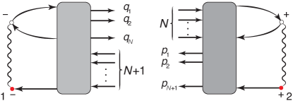
Figure 2: (Color online) Diagrammatic structure of the functions $S(1)$ and $S^{*}(2)$ for the lesser self-energy. The external vertex points $1$ and $2$ have times on the $-$ and $+$ branch respectively. Green’s functions are denoted by the lines with arrows, while wavy lines correspond to the bare interparticle interaction.

Thus the multiplication of a $S$ diagram by a $S^{\ast}$ diagram and the subsequent sum over $\underline{p}$ and $\underline{q}$ involves the sum over $q$ of $g_{q\mathbf{x}}^{>}g_{\mathbf{y}q}^{>}$ and the sum over $p$ of $g_{\mathbf{x}p}^{<}g_{p\mathbf{y}}^{<}$. The noninteracting lesser/greater Green’s functions can be expanded in the basis of the noninteracting one-particle eigenstates according toStefanucci and van Leeuwen (2013)

$$g^{<}_{ij}(t,t^{\prime}) = i\sum_{p}f(\epsilon_{p})e^{-i\epsilon_{p}(t-t^{\prime})}\langle i|p\rangle\langle p|j\rangle,$$ (19)

$$g^{>}_{ij}(t,t^{\prime}) = -i\sum_{q}\bar{f}(\epsilon_{q})e^{-i\epsilon_{q}(t-t^{\prime})}\langle i|q\rangle\langle q|j\rangle,$$ (20)

where $\epsilon_{p}$ is the energy of the one-particle eigenstate $|p\rangle$, $f$ is the zero-temperature Fermi function and $\bar{f}=1-f$. Taking into account that $f^{2}(\epsilon_{p})=f(\epsilon_{p})$ and $\bar{f}^{2}(\epsilon_{q})=\bar{f}(\epsilon_{q})$ one can easily verify that

$$\sum_{q}g_{\mathbf{y}q}^{>}(t_{y},\tau)g_{q\mathbf{x}}^{>}(\tau,t_{x}) = -ig^{>}_{\mathbf{y}\mathbf{x}}(t_{y},t_{x}),$$ (21)

$$\sum_{p}g_{\mathbf{x}p}^{<}(t_{x},\tau)g_{p\mathbf{y}}^{<}(\tau,t_{y}) = ig_{\mathbf{x}\mathbf{y}}^{<}(t_{x},t_{y}).$$ (22)

When taking the product of the left and the right half-diagram in Fig. 2 we can use relation (21) to replace each of the $N$ products of $g^{>}$ functions by a single $g^{>}$ connecting two internal times in each half-diagram. Similarly we can use relation (22) to replace each of the $N+1$ products of a $g^{<}$ by a single $g^{<}$. The result of this gluing procedure is a diagram with external vertices $1$ and $2$. The structure of the diagram is such that all internal vertices to the left of the glued lines have time labels on the minus branch and all internal vertices to the right of the glued lines have time labels on the plus branch. The gluing procedure can be reversed by cutting all Green’s function lines between a vertex labeled $-$ and a vertex labeled $+$. We will refer to this procedure as the cutting rule for a diagram.

At this point we observe that the self-energy in Eq. (15) is not the sum of all possible $S$-$S^{\ast}$ diagrams due to the subscript “irr”. This means that from the diagrams obtained by the gluing procedure we still have the remove the reducible diagrams, i.e., the diagrams which fall apart in two disjoint pieces by cutting a single Green’s function line. An obvious case of a reducible diagram is when there is only a single line to glue in Fig. 2. This happens when $N=0$ and we only have the single label $p_{1}$. This case is easily taken care of by letting the sum in Eq. (15) start at $N=1$ instead. For $N>1$ the gluing procedure leads to reducible diagrams whenever the $S$-diagram can be disjoint into a piece which contains only vertex 1 and a piece which contains the $\underline{p}\underline{q}$ vertices by cutting a single Green’s function line. We call these $S$-diagrams reducible and define $\tilde{S}$ as the sum of irreducible $S$-diagrams. Note that the $\tilde{S}$-diagrams can be disjoint into two pieces by cutting a single Green’s function line, but then one of the pieces would contain 1 and some of the $\underline{p}\underline{q}$ vertices. For instance half-diagrams with a self-energy insertion on the lines we glue together belong to $\tilde{S}$. An example is shown in Fig. 3 where a tadpole in inserted in one of the $p$-lines. This half-diagram can be disjoint by a single cut but then the vertex 1 would not be isolated from all the $\underline{p}\underline{q}$. Consequently this half-diagram belongs to $\tilde{S}$ and produces irreducible diagrams for the self-energy.

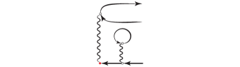
Figure 3: (Color online) Minimal example of irreducible $S$ diagram with self-energy insertions. When glued with some irreducible $S^{\ast}$ diagram it yields an irreducible self-energy diagram. Notice that this diagram is reducible in the “correlation function” sense because cutting a single Green’s function line produces disconnected pieces.

From this analysis we conclude that the self-energy can be written as

$$\Sigma_{c}^{<}(1,2)=i\sum_{N=1}^{\infty}\frac{1}{(N+1)!N!}\sum_{\underline{p}\underline{q}}\tilde{S}_{N,\underline{p}\underline{q}}(2)\tilde{S}_{N,\underline{p}\underline{q}}^{*}(1).\;\;\;\;\;$$ (23)

Equation (23) is the Lehmann-like representation of the self-energy and the main result of this section. The irreducible part of products in Eq. (15) has been transformed into products of irreducible parts in Eq. (23). The product of a $\tilde{S}$-diagram and a $\tilde{S}^{\ast}$-diagram yields an irreducible self-energy diagram in which the internal times are either integrated over the minus-branch or over the plus-branch. We call this product a partition of the self-energy diagram. It is now easy to show that the Fourier transform of $-i\Sigma_{c}^{<}$ has the PSD property. Fourier transforming $\tilde{S}$ and $\tilde{S}^{\ast}$ and omitting the dependence on the position-spin variables we find

$$-i\Sigma_{c}^{<}(1,2) = \sum_{N=1}^{\infty}\frac{1}{(N+1)!N!}\int\frac{d\omega}{2\pi}\frac{d\omega^{\prime}}{2\pi}$$ (24)

$$e^{-i\omega t_{2}+i\omega^{\prime}t_{1}}\sum_{\underline{p}\underline{q}}\tilde{S}_{N,\underline{p}\underline{q}}(\omega)\tilde{S}_{N,\underline{p}\underline{q}}^{*}(\omega^{\prime}).\quad\quad$$

In this equation the Fourier transform of $\tilde{S}(t_{2})$ (and similarly of $\tilde{S}^{\ast}(t_{1})$) is performed over the time argument $t_{2}$ and not over the time difference $t_{2}-\tau$, which is ill-defined for $\tau\rightarrow\infty$. For the right hand side to depend only on $t_{1}-t_{2}$ the following property

$$\sum_{N=1}^{\infty}\frac{1}{(N+1)!N!}\sum_{\underline{p}\underline{q}}\tilde{S}_{N,\underline{p}\underline{q}}(\omega)\tilde{S}_{N,\underline{p}\underline{q}}^{*}(\omega^{\prime})=\mathcal{F}(\omega)\delta(\omega-\omega^{\prime})$$

has to be fulfilled. From this property we see that $\mathcal{F}(\omega)\geq 0$ and inserting it back into equation (24) we see that $\mathcal{F}(-\omega)$ is the Fourier transform of the function $-i\Sigma_{c}^{<}(1,2)$ with respect to the time difference $t_{1}-t_{2}$.

So far we have restricted ourselves to the exact self-energy. In the following section we will explain how a given approximate diagrammatic expression for the self-energy can be extended, if necessary, to a similar form as in Eq. (23) by an appropriate selection of additional half-diagrams, thereby ensuring the positivity of its spectral function.

II.2 Diagrammatic theory of positive spectral functions

The Lehmann-like representation of Eq. (23) brings to light a general and simple rule to calculate the lesser component of a self-energy diagram. A diagram for $\Sigma^{<}_{c}(1,2)$ has two external vertices, one with time $t_{1}$ on the minus-branch and the other with time $t_{2}$ on the plus-branch, and a certain number of internal vertices with times to be integrated over the Keldysh contour. If we assign to each internal vertex a $-$ or a $+$ sign to signify that the corresponding time is integrated over the minus or plus branch then we obtain a division of the original self-energy diagram, and the full self-energy diagram is the sum of all of them. Since the two-particle interaction is local in time, i.e.,

$$v(\mathbf{x}_{1}t_{1},\mathbf{x}_{2}t_{2})=v(\mathbf{x}_{1},\mathbf{x}_{2})\delta(t_{2}-t_{1}),$$

it only connects two vertices with times on the same branch of the Keldysh contour. Since the external vertices are fixed there are $2^{n-2}$ divisions ($n>1$) for a diagram with $n$ interaction lines. However, not all such divisions contribute. As shown in Fig. 2 and in Eq. (23) the only divisions appearing in the expansion of the self-energy are those in which one side of the diagram only contains “$-$” vertices and the other side of the diagram only contains “$+$” vertices. All other divisions must therefore be discarded. These are the divisions for which we get a piece disconnected from the external vertices 1 and 2 upon cutting the $+/-$ $g$-lines (hence these divisions cannot be written as the product of a $\tilde{S}$-$\tilde{S}^{\ast}$ diagram). The number of contributing divisions clearly depends on the topological structure of the diagram. In Section II.1 we called such divisions partitions. As an example consider the $\Sigma_{c}^{<}$ diagram shown in Fig. 4. The third division vanishes since we get a piece disconnected from 1 and 2 upon cutting the $+/-$ $g$-lines. This simple diagrammatic rule to extract the lesser self-energy can be viewed as a generalization of the Langreth rules Langreth (1976) to diagrams which are neither a product nor a convolution of Green’s functions. Ness et al. (2011) The same diagrammatic rule can alternatively be derived by working in frequency space and by taking into account the conservation of energy at each vertex.Veltman (1963); Kobes and Semenoff (1985)

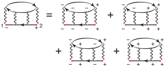
Figure 4: (Color online) An example of the distribution of $+$ and $-$ labels over the internal vertices of a lesser fourth order self-energy diagram. Divisions with lines $v^{+-}$ or $v^{-+}$ vanish due to the time-locality of the interaction and therefore are not shown. The third term after the equality sign must be discarded because it contains an isolated island of plus signs upon cutting the $+/-$ $g$-lines (see explanation in the text).

There remains one issue to address before introducing our diagrammatic theory of PSD spectral functions: How many $\tilde{S}$-$\tilde{S}^{\ast}$ diagrams do lead to the same partition of a self-energy diagram? To answer this question we need to investigate the expansion of $\tilde{S}$ in terms of Feynman diagrams. Due to the anti-commutation rules for the creation and annihilation operators it follows from the definition of $S_{N,\underline{p}\underline{q}}$ in Eq. (18) that a permutation $P$ of the labels $\underline{p}$ and a permutation $Q$ of the labels $\underline{q}$ simply changes the sign of $S_{N,\underline{p}\underline{q}}$, and hence also $\tilde{S}_{N,\underline{p}\underline{q}}$, by a factor $(-1)^{P+Q}$. Therefore if we let $\{D_{\underline{p}\underline{q}}^{(j)}\}$ with $j\in I_{N}$ be the set of all topologically inequivalent diagrams for $\tilde{S}_{N,\underline{p}\underline{q}}$ that differ by more than a permutation of the $\underline{p}$ or $\underline{q}$ labels, then we can write

$$\tilde{S}_{N,\underline{p}\underline{q}}=\sum_{j\in I_{N}}\sum_{\begin{subarray}{c}P\in\pi_{N+1}\\ Q\in\pi_{N}\end{subarray}}(-)^{P+Q}D_{P(\underline{p})Q(\underline{q})}^{(j)},$$ (25)

where $P$ and $Q$ run over all permutations $\pi_{N+1}$ and $\pi_{N}$ of $N+1$ and $N$ indices respectively. Inserting Eq. (25) back into Eq. (23) we find

$$\Sigma_{c}^{<}(1,2) = i\sum_{N=1}^{\infty}\sum_{j_{1},j_{2}\in I_{N}}\sum_{\begin{subarray}{c}P_{1},P_{2}\in\pi_{N+1}\\ Q_{1},Q_{2}\in\pi_{N}\end{subarray}}\frac{(-)^{P_{1}+Q_{1}+P_{2}+Q_{2}}}{(N+1)!N!}$$ (26)

$$\times \sum_{\underline{p}\underline{q}}D^{(j_{2})}_{P_{2}(\underline{p})Q_{2}(\underline{q})}(2)D^{(j_{1})^{*}}_{P_{1}(\underline{p})Q_{1}(\underline{q})}(1).$$

This expression can be simplified further by noticing that the composite permutations $P\circ P_{i}$ and $Q\circ Q_{i}$ with $i=1,2$ yield the same contribution as the permutations $P_{i}$ and $Q_{i}$, i.e.,

$$D^{(j_{2})}_{P\circ P_{2}(\underline{p})Q\circ Q_{2}(\underline{q})}(2)D^{(j_{1})^{*}}_{P\circ P_{1}(\underline{p})Q\circ Q_{1}(\underline{q})}(1)\\ =D^{(j_{2})}_{P_{2}(\underline{p})Q_{2}(\underline{q})}(2)D^{(j_{1})^{*}}_{P_{1}(\underline{p})Q_{1}(\underline{q})}(1),$$ (27)

since the effect of $P$ and $Q$ is equivalent to a relabeling of the $\underline{p}$ and $\underline{q}$. There are $N!(N+1)!$ such relabelings and they all give the same contribution. We can therefore simplify Eq. (26) to

$$\Sigma_{c}^{<}(1,2)=i\sum_{N=1}^{\infty}\sum_{j_{1},j_{2}\in I_{N}}\sum_{\begin{subarray}{c}P_{1}\in\pi_{N+1}\\ Q_{1}\in\pi_{N}\end{subarray}}(-)^{P_{1}+Q_{1}}\\ \times\sum_{\underline{p}\underline{q}}D^{(j_{2})}_{\underline{p}\underline{q}}(2)D^{(j_{1})^{*}}_{P_{1}(\underline{p})Q_{1}(\underline{q})}(1).$$ (28)

Every term of the form $\sum_{\underline{p}\underline{q}}D^{(j_{2})}_{\underline{p}\underline{q}}(2)D^{(j_{1})^{*}}_{P_{1}(\underline{p})Q_{1}(\underline{q})}(1)$ in Eq. (28) corresponds to a unique partition of a $\Sigma^{<}_{c}$ diagram. Vice versa, every partition of a $\Sigma^{<}_{c}$ diagram can be written as the product of a unique $D$-$D^{\ast}$ diagram for otherwise there should exist more than one way to cut the self-energy along the $+/-$ $g$-lines.

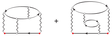
Figure 5: (Color online) An approximate self-energy of many-body perturbation theory.

Equation (28) is an exact rewriting of $\Sigma^{<}_{c}$ in terms of $D$ diagrams. MBPT approximations to the self-energy consist of the sum of a (finite or infinite) subset of diagrams. An exotic approximation could be, e.g., the one of Fig. 5. Each diagram contains four interaction lines ($n=4$) and, therefore, it is divided in $2^{n-2}=4$ different ways. It is a simple exercise to see that the left diagram is the sum of three partitions with three $+/-$ $g$-lines and one partition with five $+/-$ $g$-lines whereas the right diagram is the sum of two partitions with three $+/-$ $g$-lines and two partitions with five $+/-$ $g$-lines. In Fig. 6 we display, e.g., all partitions with five $+/-$ $g$-lines ($N=2$ in Eq. (28)) and how to write them as $D$-$D^{\ast}$ diagrams. There are two different $D$ diagrams, say $D^{(a)}$ and $D^{(b)}$, which are glued as

$$\sum_{\underline{p}\underline{q}}\left[D^{(a)}_{p_{1}p_{2}p_{3}q_{1}q_{2}}(2)\left(D^{(b)^{\ast}}_{p_{1}p_{2}p_{3}q_{1}q_{2}}(1)-D^{(b)^{\ast}}_{p_{1}p_{2}p_{3}q_{2}q_{1}}(1)\right)\right.$$

$$\left.-D^{(b)}_{p_{1}p_{2}p_{3}q_{1}q_{2}}(2)D^{(a)^{\ast}}_{p_{1}p_{2}p_{3}q_{2}q_{1}}(1)\right].$$

The products of the half-diagrams is represented in the same order as they appear in this mathematical expression in Fig. 6 after the equality sign. The diagrams $D^{(b)}$ in the first line differ only in a permutation of the labels $q_{1}$ and $q_{2}$ as shown in the left half-diagrams of Fig. 6. Furthermore, the right half-diagram of the first term ($D^{(a)}$) and the left half-diagram of the last term ($D^{(a)^{\ast}}$) have the same topological structure but differ in the labeling of $q_{1}$ and $q_{2}$.

This example is instructive since it highlights the general structure of a MBPT approximation to the self-energy. The partitioning leads to an expression of the form of Eq. (28) where the domains of the summation indices and the set of permutations are restricted. The couple $(j_{1},j_{2})$ runs over a subset $\mathcal{I}_{N}\subset I_{N}\times I_{N}$ of the product set of the topologically inequivalent half-diagrams. In the example of Fig. 6 we have $\mathcal{I}_{2}=\{(a,b),(b,a)\}$. Given the couple $(j_{1},j_{2})\in\mathcal{I}_{N}$ the permutations $P_{1}$ and $Q_{1}$ run over a subset $\pi_{N+1,p}^{(j_{1}j_{2})}\subset\pi_{N+1}$ and $\pi_{N,q}^{(j_{1}j_{2})}\subset\pi_{N}$ of the permutation groups $\pi_{N+1}$ and $\pi_{N}$. In the example of Fig. 6 for the couple $(b,a)$ (the first two terms after the equality sign) we have the subsets $\pi_{3,p}^{(ba)}=\{\boldmath{1}\}$ and $\pi_{2,q}^{(ba)}=\{\boldmath{1},Q\}$ with $Q(q_{1},q_{2})=(q_{2},q_{1})$, whereas for the couple $(a,b)$ (the last term after the equality sign) we have the subsets $\pi_{3,p}^{(ab)}=\{1\}$ and $\pi_{2,q}^{(ab)}=\{Q\}$. In Fig. 6 we considered in detail the $D$-$D^{\ast}$ diagrams of the self-energy of Fig. 5 belonging to the set $\mathcal{I}_{2}$. The set $\mathcal{I}_{1}$ in which we cut three $+/-$ $g$-lines can be analyzed similarly. All other sets $\mathcal{I}_{N}$ with $N>2$ are empty in this case. In general, however, we have for an approximate MBPT self-energy

$$\Sigma_{c}^{<}(1,2) = i\sum_{N=1}^{\infty}\sum_{(j_{1},j_{2})\in\mathcal{I}_{N}}\sum_{\begin{subarray}{c}P_{1}\in\pi^{(j_{1}j_{2})}_{N+1,p}\\ Q_{1}\in\pi^{(j_{1}j_{2})}_{N,q}\end{subarray}}(-)^{P_{1}+Q_{1}}$$ (29)

$$\times \sum_{\underline{p}\underline{q}}D^{(j_{2})}_{\underline{p}\underline{q}}(2)D^{(j_{1})^{*}}_{P_{1}(\underline{p})Q_{1}(\underline{q})}(1),$$

where the sets $\mathcal{I}_{N}$ may contain zero, a finite or an infinite number of elements.

An important remark to be made regarding Eq. (29) is that it does not, in general, fulfill the PSD property.

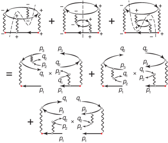
Figure 6: (Color online) Partitions of the self-energy diagrams of Fig. 5 with five $+/-$ $g$-lines and decomposition in terms of $D$-$D^{\ast}$ diagrams.

Our analysis shows, however, how to formulate the diagrammatic rules to transform a MBPT self-energy into a PSD self-energy by adding the minimal number of partitions. For the PSD property to be fulfilled the self-energy should have the structure of Eq. (23) with some approximate $\tilde{S}_{N,\underline{p}\underline{q}}$. Let $\tilde{I}_{N}\subset I_{N}$ be the smallest subset such that

$$\tilde{I}_{N}\times\tilde{I}_{N}\supset\mathcal{I}_{N},$$ (30)

and $\tilde{\pi}_{N+1,p}$ and $\tilde{\pi}_{N,q}$ be the smallest subgroups of the permutation groups $\pi_{N+1}$ and $\pi_{N}$ with the property

$$\tilde{\pi}_{N+1,p}\supset\bigcup_{(j_{1},j_{2})\in\mathcal{I}_{N}}\pi^{(j_{1}j_{2})}_{N+1,p}\;,$$ (31)

$$\tilde{\pi}_{N,q}\supset\bigcup_{(j_{1},j_{2})\in\mathcal{I}_{N}}\pi^{(j_{1}j_{2})}_{N,q}.$$ (32)

Mathemetically $\tilde{\pi}_{N+1,p}$ and $\tilde{\pi}_{N,q}$ are given by the intersection of all subgroups containing the subsets $\pi^{(j_{1}j_{2})}_{N+1,p}$ and $\pi^{(j_{1}j_{2})}_{N,q}$. The self-energy

$$\Sigma_{c,\rm PSD}^{<}(1,2) = i\sum_{N=1}^{\infty}\sum_{j_{1},j_{2}\in\tilde{I}_{N}}\sum_{\begin{subarray}{c}P_{1}\in\tilde{\pi}_{N+1,p}\\ Q_{1}\in\tilde{\pi}_{N,q}\end{subarray}}(-)^{P_{1}+Q_{1}}$$ (33)

$$\times \sum_{\underline{p}\underline{q}}D^{(j_{2})}_{\underline{p}\underline{q}}(2)D^{(j_{1})^{*}}_{P_{1}(\underline{p})Q_{1}(\underline{q})}(1)$$

contains all partitions of Eq. (29) plus other partitions, and each partition is counted only once. Furthermore, taking into account that $\tilde{\pi}_{N+1,p}$ and $\tilde{\pi}_{N,q}$ are two subgroups, Eq. (27) is valid for all $P\in\tilde{\pi}_{N+1,p}$ and $Q\in\tilde{\pi}_{N,q}$. Hence we can rewrite Eq. (33) to bring out its product structure. We have

$$\Sigma_{c,,\rm PSD}^{<}(1,2) = i\sum_{N=1}^{\infty}\sum_{j_{1},j_{2}\in\tilde{I}_{N}}\sum_{\begin{subarray}{c}P_{1},P_{2}\in\tilde{\pi}_{N+1,p}\\ Q_{1},Q_{2}\in\tilde{\pi}_{N,q}\end{subarray}}\!\!\!\!\!\!\frac{(-)^{P_{1}+Q_{1}+P_{2}+Q_{2}}}{d_{N+1,p}d_{N,q}}$$ (34)

$$\times \sum_{\underline{p}\underline{q}}D^{(j_{2})}_{P_{2}(\underline{p})Q_{2}(\underline{q})}(2)D^{(j_{1})^{*}}_{P_{1}(\underline{p})Q_{1}(\underline{q})}(1),$$

where $d_{N+1,p}$ and $d_{N,q}$ are the dimensions of the subgroups $\tilde{\pi}_{N+1,p}$ and $\tilde{\pi}_{N,q}$ respectively. The self-energy in Eq. (34) is clearly PSD. It is also clear that any reduction of the sets $\tilde{I}_{N}$, $\tilde{\pi}_{N+1,p}$ and $\tilde{\pi}_{N,q}$ would either not include the original MBPT diagrams or would not fulfill the PSD property. Thus Eq. (34) contains the minimal number of partitions of self-energy diagrams to correct the MBPT self-energy.

This concludes the diagrammatic theory to generate PSD spectral functions. In the next sections we work out explicitly some text-book examples and derive the leading PSD self-energy diagrams with vertex corrections and screened interaction, thus going beyond the GW approximation.

II.3 Self-consistency

Before we discuss some examples in detail we would first like to address the issue of self-consistency which plays an important role in so-called conserving approximations.Stefanucci and van Leeuwen (2013); Baym (1962) So far we used the noninteracting Green’s functions $g$ to evaluate the diagrams. Suppose that a specific selection of partitions guarantees the positivity of the spectral function for $\Sigma_{c,\rm PSD}^{\lessgtr}[g]$, where we indicate explicitly the functional dependence of the self-energy on $g$. Then we can use this self-energy in the Dyson equation to evaluate a new Green’s function, which we may call $G$ to distinguish it from the noninteracting $g$. In the next step we can evaluate our approximate diagrammatic expression for the self-energy in terms of $G$, i.e., we evaluate $\Sigma_{c,\rm PSD}^{\lessgtr}[G]$. The natural question to ask then is whether $\Sigma_{c,\rm PSD}^{\lessgtr}[G]$ still has the PSD property. We now demonstrate that this is indeed the case by a modification of the derivation in Sections II.1 and II.2.

The largest modification involves relations (21) and (22) since they are not valid anymore for general dressed Green’s functions. This is, for example, easily demonstrated for the exact interacting lesser Green’s function of an $N$-particle system with ground state energy $E_{0}$, which has the Lehmann representation

$$G^{<}_{\mathbf{x}\mathbf{x}^{\prime}}(t,t^{\prime})=i\sum_{\alpha}e^{-i\Omega_{\alpha}(t-t^{\prime})}f_{\alpha}(\mathbf{x})f_{\alpha}^{*}(\mathbf{x}^{\prime}).$$ (35)

Here $\alpha$ labels the many-body eigenstates $\Psi_{\alpha,N-1}$ with energy $E_{\alpha,N-1}$ of the system with $N-1$ particles, $\Omega_{\alpha}=E_{\alpha,N-1}-E_{0,N}$ are the removal energies and $f_{\alpha}(\mathbf{x})=\langle\Psi_{\alpha,N-1}|\hat{\psi}(\mathbf{x})|\Psi_{0}\rangle$ the so-called Dyson orbitals. Although the Lehmann representation (35) looks formally identical to the expansion in Eq. (19) for $g$, it does not allow us to derive Eq. (21) anymore since the nonvanishing $f_{\alpha}(\mathbf{x})$ form an overcomplete and nonorthonormal one-particle basis-set (in a noninteracting system most $f_{\alpha}(\mathbf{x})$ are zero and the nonvanishing ones form an orthonormal basis-set). Our strategy, therefore, is to replace Eqs. (19) and (20) with a different relation that still allows us to formulate a cutting rule. Crucial in our reasoning is that a PSD self-energy generates a PSD spectral function for $G$, as was explained just below Eq. (8). This implies that $G^{<}$ has the form

$$G_{\mathbf{x}\mathbf{x}^{\prime}}^{<}(t,t^{\prime})=i\int\frac{d\omega}{2\pi}\,A^{<}_{\mathbf{x}\mathbf{x}^{\prime}}(\omega)\,e^{-i\omega(t-t^{\prime})}$$

where the removal-part of the spectral function $A^{<}_{\mathbf{x}\mathbf{x}^{\prime}}(\omega)\equiv f(\omega)A_{\mathbf{x}\mathbf{x}^{\prime}}(\omega)$ is a self-adjoint and PSD matrix in the one-particle indices for every $\omega$. Denoting by $\langle\mathbf{x}|a_{i}(\omega)\rangle$ the eigenstates of $A^{<}_{\mathbf{x}\mathbf{x}^{\prime}}(\omega)$ with eigenvalue $a_{i}(\omega)$, the spectral representation of this matrix can be written as

$$A_{\mathbf{x}\mathbf{x}^{\prime}}^{<}(\omega)=\sum_{i}\langle\mathbf{x}|a_{i}(\omega)\rangle\,a_{i}(\omega)\langle a_{i}(\omega)|\mathbf{x}^{\prime}\rangle.$$

Without loss of generality we shall assume that the eigenstates $|a_{i}(\omega)\rangle$ form an orthonormal basis-set for every $\omega$. Due to the PSD property of $A^{<}$ the eigenvalues $a_{i}\geq 0$, and therefore we can define the square root of the spectral function according to

$$\sqrt{A^{<}}_{\,\mathbf{x}\mathbf{x}^{\prime}}(\omega)=\sum_{i}\langle\mathbf{x}|a_{i}\rangle\,\sqrt{a_{i}}\;\langle a_{i}|\mathbf{x}^{\prime}\rangle$$

where for notational convenience we suppressed the $\omega$-dependence of the eigenvalues and eigenvectors. Correspondingly we can define the square root of the lesser Green’s function according to

$$\sqrt{G^{<}}_{\,\mathbf{x}\mathbf{x}^{\prime}}(t,t^{\prime})=i\int\frac{d\omega}{2\pi}\,\sqrt{A^{<}}_{\,\mathbf{x}\mathbf{x}^{\prime}}(\omega)\,e^{-i\omega(t-t^{\prime})}.$$

This function has the property that

$$iG^{<}_{\mathbf{x}\mathbf{x}^{\prime}}(t,t^{\prime})=\int\!d\mathbf{y}d\bar{t}\;\sqrt{G^{<}}_{\;\mathbf{x}\mathbf{y}}(t,\bar{t})\sqrt{G^{<}}_{\mathbf{y}\mathbf{x}^{\prime}}(\bar{t},t^{\prime})$$ (36)

as follows from a quick calculation using the definitions above. Similarly $G^{>}$ is the integral over a positive spectral function, and we can therefore define the square root $\sqrt{G^{>}}$ with the property that

$$-iG^{>}_{\mathbf{x}\mathbf{x}^{\prime}}(t,t^{\prime})=\int\!d\mathbf{y}d\bar{t}\;\sqrt{G^{>}}_{\mathbf{x}\mathbf{y}}(t,\bar{t})\sqrt{G^{>}}_{\mathbf{y}\mathbf{x}^{\prime}}(\bar{t},t^{\prime}).$$ (37)

The relations (36) and (37) provide a new cutting rule for a self-energy diagram with a dressed Green’s function. Whenever we cut a self-energy diagram we obtain half-diagrams with outgoing lines $\sqrt{G^{<}}$ and $\sqrt{G^{>}}$. Using these modified half-diagrams we obtain an equation that is identical in structure to Eq. (33). The only thing that changes in Eq. (33) is that the sums over $\underline{p}\underline{q}$ are replaced by integrals over $\mathbf{y}$’s and $\bar{t}$’s. However this does not change the quadratic structure of the equation. We therefore conclude that $\Sigma_{c,\rm PSD}^{<}[G]$ also is PSD. From this new self-energy we can use the Dyson equation to calculate a new Green’s function which has again a PSD spectral function and can be decomposed as in Eqs. (36) and (37), thereby yielding yet another PSD self-energy. By repeating the procedure we obtain a series of PSD Green’s functions. If this series converges to a limiting Green’s function then we have solved the Dyson equation self-consistently for our approximate $\Sigma_{c,\rm PSD}^{<}$ in which both the Green’s function and the self-energy are PSD.

The conclusion of this analysis is that our diagrammatic approach to PSD spectral functions also applies to self-consistent perturbation theory. Of course, in order to avoid double countings, the partitions of which $\Sigma^{<}_{c,\rm PSD}$ is made of should be skeletonic, i.e., should not contain self-energy insertions.Stefanucci and van Leeuwen (2013) An important approximation that has this structure is the GW approximation which we study in more detail below. In general, however, it should be emphasized that a PSD self-energy made exclusively of all the partitions of conserving diagrams is rare. In fact, approximations which are simultaneously conserving and PSD are exceptional.

III Examples

In this section we apply the formalism developed in Section II to some illustrative examples.

Single bubble diagram

Let us first consider the first bubble diagram shown in Fig. 7(A). The lesser component of this self-energy reads

$$\Sigma_{c}^{<}(1,2) = \int d\mathbf{x}_{3}\int d\mathbf{x}_{4}v(\mathbf{x}_{1},\mathbf{x}_{3})g^{<}_{\mathbf{x}_{1}\mathbf{x}_{2}}(t_{1},t_{2})$$ (38)

$$\times g^{<}_{\mathbf{x}_{3}\mathbf{x}_{4}}(t_{1},t_{2})g^{>}_{\mathbf{x}_{4}\mathbf{x}_{3}}(t_{2},t_{1})v(\mathbf{x}_{2},\mathbf{x}_{4})$$

which can be partitioned in only one way. Upon cutting along the $+/-$ $g$-lines we find

$$\Sigma^{<}_{c}(1,2)=i\sum_{\underline{p}\underline{q}}D_{p_{1}p_{2}q_{1}}^{(a)}(2)D^{(a)^{*}}_{p_{1}p_{2}q_{1}}(1),$$ (39)

where the $D$ diagram reads

$$D^{(a)^{*}}_{p_{1}p_{2}q_{1}}(1) = \int d\mathbf{x}_{3}v(\mathbf{x}_{1},\mathbf{x}_{3})g^{<}_{\mathbf{x}_{1}\,p_{1}}(t_{1},\tau)$$ (40)

$$\times g^{<}_{\mathbf{x}_{3}\,p_{2}}(t_{1},\tau)g^{>}_{q_{1}\,\mathbf{x}_{3}}(\tau,t_{1}).$$

Equation (39) is already of the form in Eq. (33) and therefore the first bubble diagram produces a PSD spectrum.

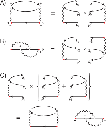
Figure 7: (Color online) (A) Partition of the first bubble diagram and the resulting half-diagrams. (B) Partition of the second-order exchange diagram and the resulting half-diagrams. (C) In order to form a a complete square with the second-order exchange diagram we need to add the right half-diagram with permuted $p_{1}$ and $p_{2}$ labels. This yields the 2B approximation.

Second-order exchange

The exchange diagram of the first bubble diagram is shown in Fig. 7(B) and the application of the formalism is more interesting. The lesser component of the self-energy now reads

$$\Sigma_{c}^{<}(1,2) = -\int d\mathbf{x}_{3}\int d\mathbf{x}_{4}v(\mathbf{x}_{1},\mathbf{x}_{3})g^{<}_{\mathbf{x}_{1}\mathbf{x}_{4}}(t_{1},t_{2})$$

$$\times g^{>}_{\mathbf{x}_{4}\mathbf{x}_{3}}(t_{2},t_{1})g^{<}_{\mathbf{x}_{3}\mathbf{x}_{2}}(t_{1},t_{2})v(\mathbf{x}_{4},\mathbf{x}_{2}).$$

This diagram too can be partitioned in only one way. However, upon cutting the $+/-$ $g$-lines we find a product of $D$ diagrams differing by a permutation $P(p_{1},p_{2})=(p_{2},p_{1})$

$$\Sigma_{c}^{<}(1,2)=i\sum_{\underline{p}\underline{q}}(-)^{P}D_{p_{1}p_{2}q_{1}}^{(a)}(2)D^{(a)^{*}}_{p_{2}p_{1}q_{1}}(1)$$

where $D_{p_{1}p_{2}q_{1}}^{(a)}$ is the same as in Eq. (40). The smallest subgroup of $\pi_{2}$ which contains $P$ is $\pi_{2}$ itself and the domain $j_{1}=a$ and $j_{2}=a$ is already of the form $\tilde{I}_{1}\times\tilde{I}_{1}$. Therefore we can form a PSD self-energy by taking $\tilde{I}_{1}=\{a\}$, $\tilde{\pi}_{2,p}=\pi_{2}$ and $\tilde{\pi}_{1,q}=\{\boldmath{1}\}=\pi_{1}$. In this way we end up with the diagrams shown in Fig. 7(C). This is the second-Born (2B) approximation, which we have now shown to give a PSD spectrum. The second-order exchange diagram is particularly instructive since it shows that the PSD outcome of the sum of MBPT diagrams is not the sum of the PSD outcome of the MBPT diagrams taken separately. Indeed the PSD outcome of the first-bubble diagram is the first bubble-diagram itself whereas the PSD outcome of the second-order exchange diagram is the 2B approximation. This implies that if we had summed the PSD outcomes of these two separate diagrams we would have counted the first-bubble diagram twice. No double counting occurs if we apply the rules in Eqs. (30-32) to the 2B approximation; the PSD outcome would be the 2B approximation itself.

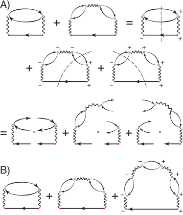
Figure 8: (Color online) (A) Partitions of the first and second bubble diagrams and the resulting half-diagrams. (B) The minimal completion of the square which yields a PSD spectrum.

Two bubbles

As a third example let us consider the sum of the first and second bubble diagrams as shown in Fig. 8(A). After distributing the pluses and minuses over the internal vertices we find that the lesser self-energy diagram can be written in terms of two types of $D$-diagrams

$$\Sigma_{c}^{<}(1,2)\!\! = \!i\sum_{\underline{p}\underline{q}}\Big{[}D_{p_{1}p_{2}q_{1}}^{(a)}(2)D_{p_{1}p_{2}q_{1}}^{(a)^{*}}(1)$$

$$+ \!\!D_{p_{1}p_{2}q_{1}}^{(b)}(2)D_{p_{1}p_{2}q_{1}}^{(a)^{*}}(1)+D_{p_{1}p_{2}q_{1}}^{(a)}(2)D_{p_{1}p_{2}q_{1}}^{(b)^{*}}(1)\Big{]}.$$

The three $D$-$D^{\ast}$ diagrams in this expression are represented in the bottom line of Fig. 8(A). We observe that the only permutation appearing is the identity permutation. Therefore, according to the rules in Eqs. (30-32), we only need to find the smallest $\tilde{I}_{1}$ such that $\tilde{I}_{1}\times\tilde{I}_{1}\supset\{(a,a),(a,b),(b,a)\}$. This is simply $\tilde{I}_{1}=\{a,b\}$. Thus, the PSD outcome of the self-energy is

$$\Sigma_{c,\rm PSD}^{<}(1,2)=\sum_{j_{1}j_{2}\in\tilde{I}_{1}}\sum_{\underline{p}\underline{q}}D_{p_{1}p_{2}q_{1}}^{(j_{2})}(2)D_{p_{1}p_{2}q_{1}}^{(j_{1})^{\ast}}(1)$$

and the corresponding diagrams are shown in Fig. 8(B). In accordance with our notation a diagram with no plus/minus on the internal vertices represents the full diagram, i.e., the sum of all possible partitions.

GW and T-matrix approximations

With similar arguments it is easy to show that the GW self-energy has the PSD property. We take the RPA $W=v+vPW$ with

$$P_{\mathbf{x}_{1}\mathbf{x}_{2}}(z_{1},z_{2})=-ig_{\mathbf{x}_{1}\mathbf{x}_{2}}(z_{1},z_{2})g_{\mathbf{x}_{2}\mathbf{x}_{1}}(z_{2},z_{1}).$$ (41)

Then

$$W^{<} = v\left(P^{<}+P^{{\scriptscriptstyle-}{\scriptscriptstyle-}}vP^{<}+P^{<}vP^{{\scriptscriptstyle+}{\scriptscriptstyle+}}\right.$$ (42)

$$+ P^{{\scriptscriptstyle-}{\scriptscriptstyle-}}vP^{{\scriptscriptstyle-}{\scriptscriptstyle-}}vP^{<}+P^{{\scriptscriptstyle-}{\scriptscriptstyle-}}vP^{<}vP^{{\scriptscriptstyle+}{\scriptscriptstyle+}}+P^{<}vP^{{\scriptscriptstyle+}{\scriptscriptstyle+}}vP^{{\scriptscriptstyle+}{\scriptscriptstyle+}}$$

$$+ \left.\ldots\right)v,$$

where we took into account that if $P^{{\scriptscriptstyle+}{\scriptscriptstyle+}}$ appears to the left of $P^{<}$ and/or $P^{{\scriptscriptstyle-}{\scriptscriptstyle-}}$ appears to the right of $P^{<}$ then the division is not a partition since a cut along the $+/-$ $g$-lines generates a disconnected $+$ and/or $-$ island, see Section II.2. It is a matter of simple algebra to prove that

$$\Sigma_{\rm GW}^{<}(1,2) \equiv ig^{<}(1,2)W^{<}(1,2)$$ (43)

$$= i\sum_{j_{1}j_{2}=1}^{\infty}\sum_{\underline{p}\underline{q}}D_{p_{1}p_{2}q_{1}}^{(j_{2})}(2)D_{p_{1}p_{2}q_{1}}^{(j_{1})^{\ast}}(1),$$

where the diagrams $D^{(j)}$ are defined as in Fig. 9(A). Equation (43) is clearly of the form in Eq. (33). In a similar fashion it can be shown that the symmetrized version of the T-matrix approximation also has the PSD property since it can be written as in the second row of Eq. (43) with $D$ diagrams given in Fig. 9(B).

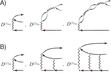
Figure 9: (Color online) (A) Partitions of the bubble diagrams of the GW approximation. (B) Partitions of the ladder diagrams of the T-matrix approximation.

IV PSD self-energy beyond GW

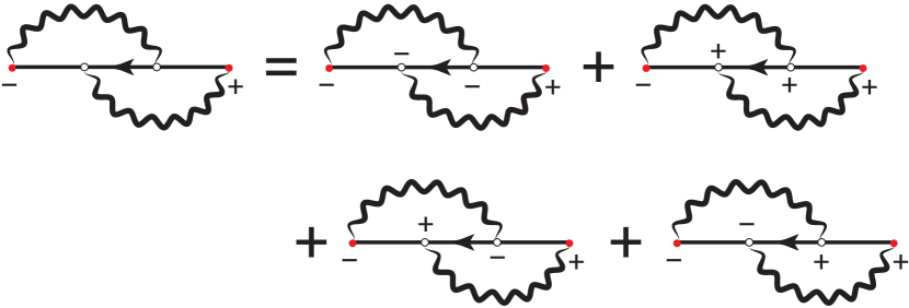
Figure 10: (Color online) Next to leading order self-energy in the screened interaction $W$. Since $W$ is non-local in time, the thick wavy lines denoting the screened interaction can connect points on different branches of the Keldysh contour.

The GW self-energy is the leading order approximation in the screened interaction $W$. Despite the numerous successful applications of the GW approximation in reproducing experimental spectra there is also a commensurable number of examples for which the GW approximation fails, pointing out the importance of including vertex corrections. The next to leading order approximation in $W$ is represented by the diagram $\Sigma_{\rm vert}$ of Fig. 10 and contains a vertex correction. Unfortunately the self-energy $\Sigma_{\rm GW+v}\equiv\Sigma_{\rm GW}+\Sigma_{\rm vert}$ is not PSD and the resulting spectral function has the undesired feature of being negative in some region of the frequency space. In this section we use the rules of Eqs. (30-32) to identify the minimal number of additional partitions for constructing the leading order beyond-GW self-energy with the PSD property.

On the right hand side of Fig. 10 the self-energy $\Sigma_{\rm vert}$ is written as the sum of four partitions. Let us determine the underlying $D$ diagrams. We observe that the screened interactions $W^{{\scriptscriptstyle+}{\scriptscriptstyle+}}$ or $W^{{\scriptscriptstyle-}{\scriptscriptstyle-}}$ can be partitioned in only one way with all internal polarizations $P^{{\scriptscriptstyle+}{\scriptscriptstyle+}}$ or $P^{{\scriptscriptstyle-}{\scriptscriptstyle-}}$. Indeed a partition of $W^{{\scriptscriptstyle+}{\scriptscriptstyle+}}$ in which appears a $P^{>}$ does necessarily contain also a $P^{<}$ and hence the cut along the $+/-$ $g$-lines would generate a disconnected island. A similar argument applies to $W^{{\scriptscriptstyle-}{\scriptscriptstyle-}}$.

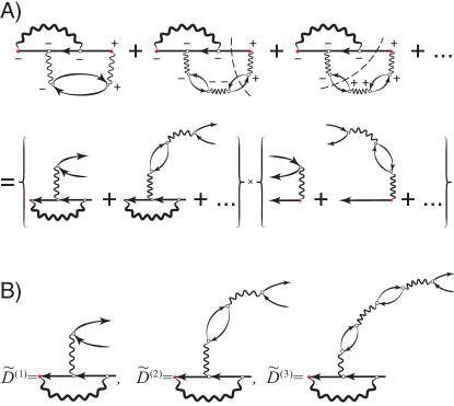
Figure 11: (Color online) (A) Partitions of the first diagram on the right hand side of Fig. 10. (B) Definition of the $\tilde{D}^{(j)}$ diagrams.

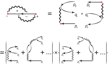
Figure 12: (Color online) Partitions of the third diagram on the right hand side of Fig. 10.

Accordingly the first diagram on the right hand side of Fig. 10 is the sum of the partitions shown in Fig. 11(A), and can be written as the sum of products between the $D^{(j)}$ diagrams of the GW approximation, see Fig. 9(A), and the $\tilde{D}^{(j)}$ diagrams displayed in Fig. 11(B). The same is true for the second diagram of Fig. 10 provided we exchange $D^{(j)}$ with $\tilde{D}^{(j)}$. The partitions of the third diagram of Fig. 10 are very simple due to the presence of only $W^{{\scriptscriptstyle+}{\scriptscriptstyle+}}$ and $W^{{\scriptscriptstyle-}{\scriptscriptstyle-}}$, see Fig. 12. The result is the sum of products between $D^{(j)}$ diagrams and permuted $D^{(j)}$ diagrams. Finally the fourth diagram of Fig. 10 is partitioned as illustrated in Fig. 13(A), and can be written as the sum of products between two $D^{(ij)}$ diagrams, see Fig. 13(B), where $i$ refers to the number of top bubbles and $j$ to the number of bottom bubbles. In conclusion (omitting the dependence on $1$ and $2$)

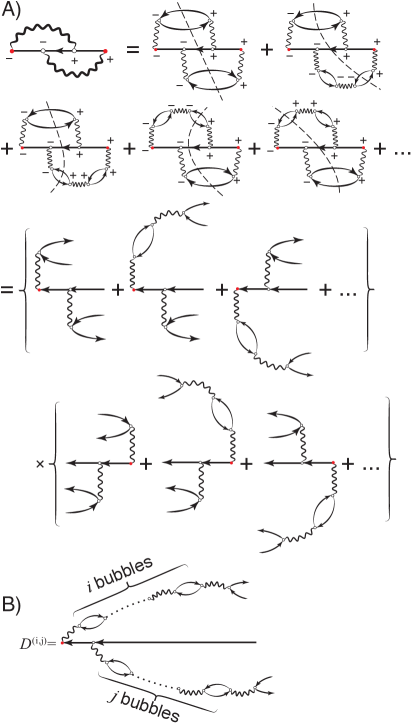
Figure 13: (Color online) (A) Partitions of the fourth diagram on the right hand side of Fig. 10. (B) Definition of the $D^{(i,j)}$ diagrams.

$$\Sigma^{<}_{\rm GW+v} = i\sum_{j_{1}j_{2}=1}^{\infty}\sum_{\underline{p}\underline{q}}\left(D^{(j_{2})}_{p_{1}p_{2}q_{1}}D^{(j_{1})^{\ast}}_{p_{1}p_{2}q_{1}}+D^{(j_{2})}_{p_{1}p_{2}q_{1}}\tilde{D}^{(j_{1})^{\ast}}_{p_{1}p_{2}q_{1}}\right.$$ (44)

$$+ \left.\tilde{D}^{(j_{2})}_{p_{1}p_{2}q_{1}}D^{(j_{1})^{\ast}}_{p_{1}p_{2}q_{1}}-D^{(j_{2})}_{p_{1}p_{2}q_{1}}D^{(j_{1})^{\ast}}_{p_{2}p_{1}q_{1}}\right)$$

$$+ i\sum_{i_{1}j_{1}i_{2}j_{2}=1}^{\infty}\sum_{\underline{p}\underline{q}}D^{(i_{2}j_{2})}_{p_{1}p_{2}p_{3}q_{1}q_{2}}D^{(i_{1}j_{1})^{\ast}}_{p_{1}p_{2}p_{3}q_{1}q_{2}}.$$

Thus $\Sigma_{\rm GW+v}$ is the sum of a contribution $\Sigma_{3}$ containing partitions with three $+/-$ $g$-lines and a contribution $\Sigma_{5}$ (the last term in Eq. (44)) containing partitions with five $+/-$ $g$-lines. From the rules in Eqs. (30-32) we see that $\Sigma_{5}$ has already a PSD structure. Instead $\Sigma_{3}$ should be corrected according to $\Sigma_{3}\to\Sigma_{3,\rm PSD}$ with

$$\Sigma^{<}_{3,\rm PSD} = i\sum_{j_{1}j_{2}=1}^{\infty}\sum_{P\in\pi_{2}}(-)^{P}\sum_{\underline{p}\underline{q}}\left(D^{(j_{2})}_{p_{1}p_{2}q_{1}}+\tilde{D}^{(j_{2})}_{p_{1}p_{2}q_{1}}\right)$$ (45)

$$\times \left(D^{(j_{1})^{\ast}}_{P(p_{1})P(p_{2})q_{1}}+\tilde{D}^{(j_{1})^{\ast}}_{P(p_{1})P(p_{2})q_{1}}\right).$$

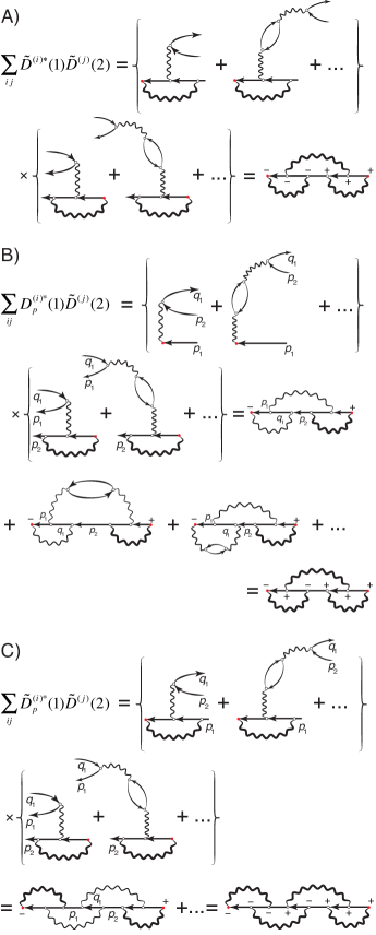
Figure 14: (Color online) There are four extra diagrams that correct the self-energy with three $+/-$ $g$-lines ($\Sigma_{3}$). They have (A) $\tilde{D}(1)\tilde{D}(2)$, (B) $D_{P}(1)\tilde{D}(2)$, $\tilde{D}_{P}(1)D(2)$ (similar to diagram (B) and thus not shown), and (C) $\tilde{D}_{P}(1)\tilde{D}(2)$ structures. Subscript $P$ denotes a diagram with permuted $p$-indices.

This self-energy contains the original four partitions of $\Sigma_{3}$ plus four more partitions arising from the permutation of the two $\underline{p}$ dangling lines. The latter are explicitly worked out in Fig. 14. Collecting all results together we conclude that the leading order self-energy diagrams with screened interactions and vertex corrections yielding a PSD spectral function are those in Fig. 15. Here we recall that a diagram with no $+/-$ on the internal vertices is the full diagram (hence the sum over all possible partitions). Noteworthy the minimal completion of the square requires a fourth order diagram in $W$.

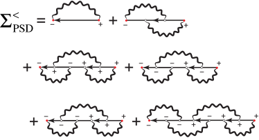
Figure 15: (Color online) Leading order beyond-GW self-energy with the PSD property. Thick wavy lines denote the screened Coulomb interaction in the random phase approximation.

V Vertex corrections in the homogeneous electron gas

The numerical implementation of the full self-energy of Fig. 15 is rather demanding. We observe, however, that the exclusion of the last partition of Fig. 10 leads to a much simpler PSD self-energy since no permuted $D$ diagrams appear. It is straightforward to show that in this case the rules of Eqs. (30-32) lead to the following PSD self-energy

$$\Sigma^{<}_{c}(1,2) = i\sum_{j_{1}j_{2}=1}^{\infty}\sum_{\underline{p}\underline{q}}\left(D^{(j_{2})}_{p_{1}p_{2}q_{1}}+\tilde{D}^{(j_{2})}_{p_{1}p_{2}q_{1}}\right)$$ (46)

$$\times \left(D^{(j_{1})^{\ast}}_{p_{1}p_{2}q_{1}}+\tilde{D}^{(j_{1})^{\ast}}_{p_{1}p_{2}q_{1}}\right),$$

where the corresponding $D$ diagrams are defined in Fig. 9(A) and Fig.  11(B). The diagrammatic representation of Eq. (46) is shown in Fig. 16. This self-energy too goes beyond the GW approximation, but the vertex correction is only partial.

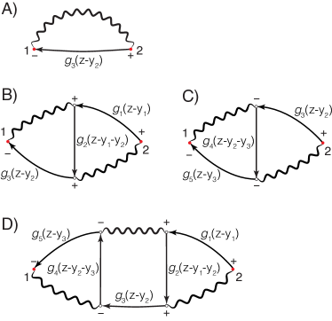
Figure 16: The sum of the four self-energy partitions A)+B)+C)+D) yields a positive spectral function. Lines with arrows denote the electron propagator $G_{0}(k,\omega)$, whereas wavy-lines stand for the screened Coulomb interaction $W_{0}(k,\omega)$. Vertices are labeled with $+$ ($-$) if the time lies on the backward (forward) branch of the Keldysh contour. Diagrams are translated into analytic expressions according to the definitions (47) and (48) and notations below Eqs. (49). For instance $g_{5}(z-y_{3})$, connecting vertices with “$-$” labels as in C) and D), corresponds to the time-ordered Green’s function (see also Eq. (2)): $\frac{\mathcal{B}(k_{5})}{z-\Omega(y_{3})-\epsilon_{k_{5}}-i\eta}+\frac{\mathcal{A}(k_{5})}{z-\Omega(y_{3})-\epsilon_{k_{5}}+i\eta}$.

The three-dimensional homogeneous electron gas (3d HEG) is one of the most studied correlated many-body system.Giuliani and Vignale (2005) We still lack detailed knowledge of one directly observable quantity – the spectral function $A(k,\omega)$ – when departing from the on-shell energy, i.e., when $\omega\not\approx\epsilon_{k}$. Discrepancies with experimental measurements contributed to the debates on the position of satellites, Holm and Aryasetiawan (1997); Aryasetiawan et al. (1996) bandwidth of simple metals, Yasuhara et al. (1999); Takada (2001) cancellation of vertex function and self-consistency effects, Minnhagen (1975); Holm and von Barth (1998); Schindlmayr and Godby (1998b) and the spectral function shape. Guzzo et al. (2011); Pavlyukh et al. (2013b)

Despite numerous efforts there are just a few results that go beyond the GW approximation in the study of quasiparticle properties. Analytically, these are the results of Onsager et al. Onsager et al. (1966) on the second-order exchange energy and of Ziesche Ziesche (2007) and of Glasser and Lamb Glasser and Lamb (2007) on the second-order exchange self-energy. These works only contain analytic results for on-shell self-energy and only a contribution of the bare Coulomb interaction is included. The screened Coulomb interaction is possible to treat numerically. The non self-consistent calculations were performed by Hedin Hedin (1965) and Lundqvist. Lundqvist (1967a, b, 1968) It took three decades to implement the same approach partially or fully self-consistently. This was achieved in works by von Barth and Holm. von Barth and Holm (1996); Holm and von Barth (1998) The non-positivity of the spectral function first observed by Minnhagen Minnhagen (1974, 1975) hindered systematic diagrammatic explorations and stimulated development of synthetic approaches: analyzing real time Kadanoff-Baym dynamics, Kwong and Bonitz (2000) neglecting the incoherent part of the electron spectral function, Shirley (1996) employing the Ward identities and a model form of the exchange-correlation kernel, Takada (2001); Takada and Yasuhara (2002); Bruneval et al. (2005); Maebashi and Takada (2011) or the self-consistent cumulant expansion. Holm and Aryasetiawan (1997)

Using the presented formalism it is now possible to pursue the diagrammatic route. In this section we present the results of a non self-consistent calculation. Thus, we evaluate the diagrams in Fig. 16 for 3d HEG using the analytical frequency and numerical Monte-Carlo momentum integrations. The method was developed in a prior publication, Pavlyukh et al. (2013b) however, especially the analytical frequency integration part had to be substantially extended. For HEG the bare time-ordered Green’s function can be written as a function of frequency $\omega$ and momentum $k$ as

$$G_{0}^{{\scriptscriptstyle-}{\scriptscriptstyle-}}(k,\omega)=\frac{\mathcal{B}(k)}{\omega-\epsilon_{k}-i\eta}+\frac{\mathcal{A}(k)}{\omega-\epsilon_{k}+i\eta}.$$ (47)

For self-consistent calculations this equation can be extended to include multiple poles (e.g., to describe quasiparticle satellites) for each momentum value. In this work we perform a one-shot calculation and therefore set $\mathcal{B}(k)=n_{k}$ and $\mathcal{A}(k)=1-n_{k}$ with $0\leq n_{k}\leq 1$ denoting the occupation number and $\epsilon_{k}$ the energy of the state with momentum $k$. For the energy dispersion we used the prescription by HedinStefanucci and van Leeuwen (2013); Hedin (1965); Hedin and Lundqvist (1970) to put the pole of the dressed $G=G_{0}+G_{0}\Sigma_{c}[G_{0}]G$ with Fermi momentum $k=k_{F}$ correctly at the Fermi surface, i.e., $\epsilon_{k}=k^{2}/2+\mu-\epsilon_{F}$ where $\mu$ is the chemical potential and $\epsilon_{F}=k_{F}^{2}/2$ is the Fermi energy. Analogous definitions have been used for the anti-time-ordered, lesser and greater Green’s functions.

Generally, each interaction line in Fig. 16 can designate either the bare Coulomb interaction or include scattering with generation of a plasmon or a particle-hole pair. On the RPA level the plasmon oscillator strength $t(q)$ vanishes when its dispersion curve $\Omega(q)$ enters the particle-hole continuum at the critical wave number $q_{c}$. Because plasmonic excitations exist on the bounded momentum interval they are especially convenient for numerics: momentum integrations need to be performed on the finite interval. Physically, plasmons also dominate the particle-hole response in electron liquids with typical metallic densities. Therefore, in present work we only treat the plasmonic contributions. The screened Coulomb interaction is treated in the plasmon pole approximation, i.e. $W(k,\omega)\approx W_{0}(k,\omega)$ (cf. Eq. 25.11 of Ref. Hedin and Lundqvist, 1970):

$$W_{0}^{--}(k,\omega)=\frac{v(k)}{2}\!\left[\frac{w(k)}{\omega-\Omega(k)+i\eta}-\frac{w(k)}{\omega+\Omega(k)-i\eta}\right],$$ (48)

where we denote $w(q)=t(q)\Omega^{2}(0)/\Omega(q)$ and $0\leq t(q)\leq 1$ is the plasmonic spectral weight with $t(0)=1$ and $t(q_{c})=0$. Analogous defininitions have been used for the other Keldysh components of $W_{0}$. Our numerical approach also allows us to include contributions from the particle-hole continuum to exhaust the $f$-sum rule for the dielectric function $\varepsilon(q,\omega)$:

$$\int_{0}^{\infty}\omega\,\mathrm{Im}\varepsilon^{-1}(q,\omega)\,d\omega=-\frac{\pi}{2}\Omega^{2}(0),$$

where $\Omega(0)=4\sqrt{\frac{\alpha r_{s}}{3\pi}}\epsilon_{F}$, with $\alpha=[4/(9\pi)]^{1/3}\approx 0.521$ and $r_{s}=1/(\alpha k_{F})$ the Wigner-Seitz radius. Monte-Carlo momentum integration of these terms is, however, more involved as it requires an extra integration for each interaction line.

The frequency integrations can be done completely analytically (facilitated by the mathematica computer algebra system) whereas for the remaining momentum integrations one has to rely on numerics. The frequency integration is implemented for a general case of time-ordered $G_{0}(k,\omega)$ and $W_{0}(k,\omega)$. Since each correlator in the self-energy expression comprises two terms the total number of terms grows geometrically with the diagrams order. In order to optimize the calculation we implemented an approach where for each $\omega$-integration the program closes the integration contour in such a way that the least number of terms is generated. One might argue that the Hedin set of equations gives a prescription on which half of the complex plane the integration should be closed (see for example Eqs. (A30) of Ref. Hedin, 1965). However, it is easy to verify that this is only relevant for the first order term. Higher order terms decay faster than $1/\omega$ at infinity ($\omega$ here denotes the frequency to be integrated over) and, therefore, the choice of the half-plane is not important. Finally, we notice that it is sufficient to consider only the lesser self-energy. The greater self-energy component required to describe properties of the states above the Fermi level is obtained from symmetry consideration.

Our analytic approach covers the case of Fig. 16(A) diagram where all partitions are included. Other diagrams on this figure contain only a subset of the partitions of the MBPT diagrams from which they originate. The corresponding analytic expressions can be easily extracted from the general result by analyzing the frequency dependence. The overall $\omega$-dependence can readily be obtained on paper by integrating $\delta$-functions in lesser and greater correlators. Despite the omission of several partitions the final result is bulky and requires an additional simplification using $\mathcal{A}(k)+\mathcal{B}(k)=1$.

The results of frequency integration are

$$\Sigma_{A}^{<}(z,\zeta) = 2i\pi\int\!\frac{d^{3}y_{2}}{(2\pi)^{3}}B_{3}C_{2}\delta(\zeta-\epsilon_{3}+\Omega_{2}),$$ (49a)

$$\Sigma_{B}^{<}(z,\zeta) = 2i\pi\iint\!\frac{d^{3}y_{1}}{(2\pi)^{3}}\frac{d^{3}y_{2}}{(2\pi)^{3}}B_{3}C_{1}C_{2}\left[\frac{\mathcal{H}_{2}(\epsilon_{3},\Omega_{1})-\mathcal{H}_{1}(\epsilon_{3}-\Omega_{2},\Omega_{1})}{\epsilon_{2}-\epsilon_{1}-\Omega_{2}}\right]\delta(\zeta-\epsilon_{3}+\Omega_{2}),$$ (49b)

$$\Sigma_{C}^{<}(z,\zeta) = 2i\pi\iint\!\frac{d^{3}y_{3}}{(2\pi)^{3}}\frac{d^{3}y_{2}}{(2\pi)^{3}}B_{3}C_{2}C_{3}\left[\frac{\mathcal{H}_{4}(\epsilon_{3},\Omega_{3})-\mathcal{H}_{5}(\epsilon_{3}-\Omega_{2},\Omega_{3})}{\epsilon_{4}-\epsilon_{5}-\Omega_{2}}\right]\delta(\zeta-\epsilon_{3}+\Omega_{2}),$$ (49c)

$$\Sigma_{D}^{<}(z,\zeta) = 2i\pi\iiint\!\frac{d^{3}y_{1}}{(2\pi)^{3}}\frac{d^{3}y_{2}}{(2\pi)^{3}}\frac{d^{3}y_{3}}{(2\pi)^{3}}B_{3}C_{1}C_{2}C_{3}\left[\frac{\mathcal{H}_{2}(\epsilon_{3},\Omega_{1})-\mathcal{H}_{1}(\epsilon_{3}-\Omega_{2},\Omega_{1})}{\epsilon_{2}-\epsilon_{1}-\Omega_{2}}\right]$$ (49d)

$$\quad\quad\quad\times\left[\frac{\mathcal{H}_{4}(\epsilon_{3},\Omega_{3})-\mathcal{H}_{5}(\epsilon_{3}-\Omega_{2},\Omega_{3})}{\epsilon_{4}-\epsilon_{5}-\Omega_{2}}\right]\ \delta(\zeta-\epsilon_{3}+\Omega_{2}),$$

where we define

$$\mathcal{H}_{i}(a,\Omega)=\frac{A_{i}}{a-\Omega-\epsilon_{i}}+\frac{B_{i}}{a+\Omega-\epsilon_{i}}.$$

In these equations we adopt the following notations: $A_{i}\equiv\mathcal{A}(x_{i})$, $B_{i}\equiv\mathcal{B}(x_{i})$, $C_{i}\equiv\frac{1}{2}v(y_{i})w(y_{i})$. The quantities $\epsilon_{i}$ and $\Omega_{i}$ are energies labeled by the momenta, as shown in Fig. 16, and have a meaning of electron and plasmon dispersions, respectively. The momenta $y_{i}$ are associated with plasmonic excitations. Eq. (49) possesses some symmetries: Eqs. (49b) and (49c) are identical upon simultaneous permutations of the $(1,5)(2,4)$ fermionic and $(1,3)$ bosonic indices. The two brackets in Eq. (49d) transform analogously. For the numerical momentum integration of Eqs. (49) it is useful to rescale the variables as follows: $k=k_{F}\,\tilde{k}$, $\epsilon_{k}=\epsilon_{F}\,\tilde{k}^{2}$, $v(q)\equiv\frac{4\pi}{q^{2}}=\frac{4\pi}{k_{F}^{2}}\,\frac{1}{\tilde{q}^{2}}$, $\Sigma=\epsilon_{F}\tilde{\Sigma}$. This leads to the following density-dependent prefactors:

$$c_{i}=\left[\left(\frac{k_{F}}{2\pi}\right)^{3}\frac{1}{\epsilon_{F}^{2}}\left(\frac{1}{2}\frac{4\pi}{k_{F}^{2}}\epsilon_{F}\right)\right]^{i}=\left(\frac{\alpha r_{s}}{2\pi^{2}}\right)^{i},$$ (50)

where $i=1,2,3$ denotes the diagram’s order.

From the particle-hole symmetry we can obtain the greater self-energy ($\Sigma^{>}$). For this it is sufficient to replace $B_{i}$ with $A_{i}$ and vice versa, and to change the sign of each $\Omega_{i}$.

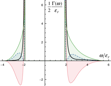
Figure 17: (Color online) The rate operator $\frac{1}{2}\Gamma(k,\omega)=-\text{Im}\,\Sigma^{\rm R}_{c}(k,\omega)$ of the homogeneous electron gas at the density of $r_{s}=4$ and $k=k_{F}$ (the energy $\omega$ is measured with respect to $\mu$). Different line-styles denote contributions of different orders: full, dotted and dashed lines stand for first, second and third order, respectively. Thick solid line denotes the sum of all contributions.

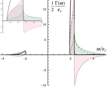
Figure 18: (Color online) The rate operator $\frac{1}{2}\Gamma(k,\omega)=-\text{Im}\,\Sigma^{\rm R}_{c}(k,\omega)$ as in Fig. 17 for a different momentum $k=1.2k_{F}$ (the energy $\omega$ is measured with respect to $\mu$). The inset magnifies the region of the logarithmic singularity. Notice the almost complete cancellation of $\Sigma^{>}_{c}(k,\omega)$ for $\omega>\epsilon_{k}+\Omega(0)$.

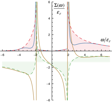
Figure 19: (Color online) The real part of the retarded self-energy $\text{Re}\,\Sigma^{\rm R}(k,\omega)$, see Eq. (52), and the rate operator $\frac{1}{2}\Gamma(k,\omega)=-\text{Im}\,\Sigma^{\rm R}_{c}(k,\omega)$ of the homogeneous electron gas at the density of $r_{s}=4$ and $k=k_{F}$ (the energy $\omega$ is measured with respect to $\mu$). Shaded dashed curves denote the first order calculation. Full lines denote contribution from diagrams shown in Fig. 16 plus the first order contribution from the particle-hole excitations. The horizontal line bounding the shaded area in the graph of $\text{Re}\,\Sigma^{\rm R}$ crosses the y-axis at the value of the exchange self-energy $\Sigma_{x}(k_{F})/\epsilon_{F}=-\frac{2\alpha}{\pi}r_{s}\approx-1.327$.

Upon a close inspection it is evident that the four terms in Eq. (49) can be combined together as follows:

$$\Sigma_{2,\text{PSD}}^{<}=2i\pi\int\!\frac{d^{3}y_{2}}{(2\pi)^{3}}B_{3}C_{2}\left[1+\int\!\frac{d^{3}y_{1}}{(2\pi)^{3}}C_{1}\frac{\mathcal{H}_{2}(\epsilon_{3},\Omega_{1})-\mathcal{H}_{1}(\epsilon_{3}-\Omega_{2},\Omega_{1})}{\epsilon_{2}-\epsilon_{1}-\Omega_{2}}\right]^{2}\delta(\zeta-\epsilon_{3}+\Omega_{2}).$$ (51)

The first order integrand (cf. Eq. (49a)) is multiplied by a full square. Since we know that the GW self-energy fulfills the PSD property the same holds for the sum of the four terms in Fig. 16. This analytic conclusion is numerically confirmed.

In order to make Eqs. (49) suitable for Monte-Carlo integration the following has to be done: (i) integrate in spherical coordinates with zenith direction along the $\mathbf{z}$ vector, (ii) one angular integration is trivially done ($2\pi$) because the system is isotropic, (iii) map integration variables to the interval $[0,1]$. The speed and quality of a pseudo-random number generator is very important for the present calculations. We use the Mersenne twister 19937 generator as implemented in gsl library combined with a highly efficient jump ahead method  due to Haramoto et al. Haramoto et al. (2008) for parallelization. The method is roughly 3 times faster than the standard fortran implementation. We used roughly $10^{12}$ Monte-Carlo realizations to get the full frequency dependence for each momentum value. Real self-energy parts were computed using the Hilbert transform:

$$\Sigma^{\rm R}(k,\omega)=\Sigma_{x}(k)+\int\frac{d\omega^{\prime}}{2\pi}\frac{\Gamma(k,\omega^{\prime})}{\omega-\omega^{\prime}+i\eta},$$ (52)

where $\Sigma_{x}(k)$ is the frequency independent exchange self-energy and $\Gamma(k,\omega)=i\big{[}\Sigma^{>}_{c}(k,\omega)-\Sigma^{<}_{c}(k,\omega)\big{]}=i\big{[}\Sigma^{\rm R}_{c}(k,\omega)-\Sigma^{\rm A}_{c}(k,\omega)\big{]}$ is the rate operator.

Each term of Eq. (49) was separately computed as shown in Figs. 17,18 for two values of $k$. The first order self-energy is well understood. One of its marked features is the existence of logarithmic singularities at $\omega=\epsilon_{k}\pm\Omega(0)$. Hedin and Lundqvist (1970) These singularities have never been observed in an experiment and are believed to be washed out by higher order contributions. Although our calculations do not preclude this conclusion we found that our selection of second-order terms makes the singularities even more pronounced.

The real part of the retarded self-energy of Eq. (51) is displayed in Fig. 19. We observe that the real part of the first order and the complete self-energy cross the y-axis at almost the same point which is equal to $\mu/\epsilon_{F}-1$. This implies that the higher order corrections do not change the chemical potential appreciably. As expected, the rate operator is everywhere positive despite a large negative contribution of the second order term. We notice an almost complete cancellations of different order terms beyond the singularities, i.e. $\omega>\epsilon_{k}+\Omega(0)$ for particle ($k>k_{F}$) and $\omega<\epsilon_{k}-\Omega(0)$ for hole ($k<k_{F}$) states. High accuracy of the Monte-Carlo integration was required to get the cancellations properly. This is especially important at metallic densities where different orders have comparable contributions. Due to the density scaling (see Eq. (50)) the first order self-energy becomes dominant at large densities ($r_{s}\rightarrow 0$), while the third order is largest in the correlated low density regime ($r_{s}\rightarrow\infty$).

The selection of diagrams of Fig. 16 and computed in this work in the plasmon pole approximation describes scattering processes accompanied by the emission or absorption of one plasmon. Correspondingly, the scattering operator has pronounced (more narrow in comparison with the first order result) peaks at $\omega=\epsilon_{k}\pm\Omega(0)$. But how important are the remaining contributions? The simplest first order term, absent in the plasmon pole approximation, but included in the results of Fig. 19, involves generation of a single particle-hole pair. Due to less restrictions on the available phase space for scattering it is important for $\omega\rightarrow\infty$ and also determines the life-time of quasiparticles in the vicinity of the Fermi energy. It also gives rise to secondary peaks in Fig. 19. These, however, are not related to scattering mechanisms involving generation of two plasmons. Inclusion of such processes is important for the interpretation of multiple satellites in the spectral function. To lowest order they result from the partition of the second-order self-energy diagram included in Fig. 15, but omitted in Fig. 16. Respective calculations are on the way and will be the subject of a forthcoming publication.

VI Conclusions

Approximations of MBPT to the self-energy can lead to unphysical density of states, with a negative spectral weight in some frequency region. This undesired feature entails unphysical results on the system properties and makes self-consistent calculations impossible due to a progressive deterioration of the analytic properties of the Green’s function. In 1985 Almbladh proposed a diagrammatic perturbation theory of the photoemission current, Almbladh (1985) and in a subsequent paper Almbladh (2006) he elaborated on the theory and gave a prescription how to combine diagrams of different order to get a physically sensible result: the positive-definite photoemission current. These ideas are precursors for our theory. Using the Green’s function of the Keldysh formalism we developed a method to construct manifestly PSD spectral functions. The method becomes particularly lucid when expressed in diagrammatic language as it amounts to apply a few simple drawing rules.

We derive a Lehmann-like representation of the exact self-energy and show that it is given by the sum of squares of irreducible correlators. We then elucidate the connection between the diagrammatic expansion of the irreducible correlators and MBPT. Any lesser/greater self-energy diagram can be partitioned into two halves with internal time-vertices on opposite branches of the Keldysh contour. Thus, by simply drawing diagrams and assigning a sign to the internal vertices we are able to extend to a minimal set of diagrams any MBPT approximation and to generate PSD spectral functions. Several important MBPT approximations, such as the GW or T-matrix approximations, do not require any corrections. Our theory applies equally well to diagrammatic expansions with noninteracting and with self-consistent Green’s functions because PSD self-energies do preserve the correct analytic structure.

In standard MBPT approximations the straightforward inclusion of vertex corrections inevitably ruin the PSD property and, hence, our additional diagrams must be included. Remarkably, these diagrams are of higher order. For instance, the inclusion of the full first-order vertex leads to diagrams of the fourth order in the screened interaction. Required computational power to numerically evaluate them is immense. Fortunately, excluding some partitions allows us to construct an approximation containing diagrams of maximally third order. They are feasible for numerics as our calculations for the 3d HEG demonstrate.

Even though we only presented in detail the formalism for the spectral function, the same ideas apply to the spectrum of the density response function. This extension, however, goes beyond the scope of the present work and will be presented elsewhere.

VII Acknowledgments

GS acknowledges funding by MIUR FIRB Grant No. RBFR12SW0J. YP acknowledges support by DFG-SFB762. AMU would like to thank the Alfred Kordelin Foundation for support. RvL would like to thank the Academy of Finland for support.

References

- Kadanoff and Baym (1962) L. Kadanoff and G. Baym, Quantum statistical mechanics Green’s function methods in equilibrium and nonequilibrium problems (W.A. Benjamin, New York, 1962).
- Stefanucci and van Leeuwen (2013) G. Stefanucci and R. van Leeuwen, Nonequilibrium Many-Body Theory of Quantum Systems: A Modern Introduction (Cambridge University Press, Cambridge, 2013).
- Hedin (1965) L. Hedin, Phys. Rev. 139, A796 (1965).
- Aulbur et al. (2000) W. G. Aulbur, L. Jonsson, and J. W. Wilkins, Solid State Phys.: Adv. Res. Appl. 54, 1 (2000).
- Holm and von Barth (1998) B. Holm and U. von Barth, Phys. Rev. B 57, 2108 (1998).
- Mahan (1994) G. D. Mahan, Comments Cond. Mat. Phys. 16, 333 (1994).
- Hong and Mahan (1994) S. Hong and G. D. Mahan, Phys. Rev. B 50, 8182 (1994).
- Verdozzi et al. (1995) C. Verdozzi, R. W. Godby, and S. Holloway, Phys. Rev. Lett. 74, 2327 (1995).
- deGroot et al. (1996) H. J. deGroot, R. T. M. Ummels, P. A. Bobbert, and W. van Haeringen, Phys. Rev. B 54, 2374 (1996).
- Minnhagen (1974) P. Minnhagen, J. Phys. C 7, 3013 (1974).
- Del Sole et al. (1994) R. Del Sole, L. Reining, and R. W. Godby, Phys. Rev. B 49, 8024 (1994).
- Shirley (1996) E. L. Shirley, Phys. Rev. B 54, 7758 (1996).
- Ness et al. (2011) H. Ness, L. K. Dash, M. Stankovski, and R. W. Godby, Phys. Rev. B 84, 195114 (2011).
- Takada (2001) Y. Takada, Phys. Rev. Lett. 87, 226402 (2001).
- Takada and Yasuhara (2002) Y. Takada and H. Yasuhara, Phys. Rev. Lett. 89, 216402 (2002).
- Romaniello et al. (2009) P. Romaniello, S. Guyot, and L. Reining, J. Chem. Phys. 131, 154111 (2009).
- Schindlmayr and Godby (1998a) A. Schindlmayr and R. W. Godby, Phys. Rev. Lett. 80, 1702 (1998a).
- Schindlmayr et al. (1998) A. Schindlmayr, T. J. Pollehn, and R. W. Godby, Phys. Rev. B 58, 12684 (1998).
- Almbladh (2006) C.-O. Almbladh, J. Phys. Conf. Ser. 35, 127 (2006).
- Danielewicz (1984) P. Danielewicz, Annals of Physics 152, 239 (1984).
- Keldysh (1965) L. V. Keldysh, Sov. Phys. JETP 20, 1018 (1965).
- Källén (1952) G. Källén, Helvetica Physica Acta 25, 417 (1952).
- Lehmann (1954) H. Lehmann, Il Nuovo Cimento 11, 342 (1954).
- Cutkosky (1960) R. E. Cutkosky, J. Math. Phys. 1, 429 (1960).
- Veltman (1963) M. Veltman, Physica 29, 186 (1963).
- Kobes and Semenoff (1985) R. L. Kobes and G. W. Semenoff, Nucl. Phys. B 260, 714 (1985).
- Kobes and Semenoff (1986a) R. L. Kobes and G. W. Semenoff, Nucl. Phys. B 272, 329 (1986a).
- Kobes and Semenoff (1986b) R. Kobes and G. Semenoff, Phys. Rev. B 34, 4338 (1986b).
- Jeon (1993) S. Jeon, Phys. Rev. D 47, 4586 (1993).
- Danielewicz (1990) P. Danielewicz, Annals of Physics 197, 154 (1990).
- Pavlyukh et al. (2013a) Y. Pavlyukh, J. Berakdar, and A. Rubio, Phys. Rev. B 87, 125101 (2013a).
- Ethofer and Schuck (1969) S. Ethofer and P. Schuck, Zeitschrift für Physik 228, 264 (1969).
- Winter (1972) J. Winter, Nucl. Phys. A 194, 535 (1972).
- Langreth (1976) D. C. Langreth, in Linear and Nonlinear Electron Transport in Solids, edited by J. Devreese and V. Doren (Springer US, 1976), vol. 17 of NATO Advanced Study Institutes Series, pp. 3–32.
- Baym (1962) G. Baym, Phys. Rev. 127, 1391 (1962).
- Giuliani and Vignale (2005) G. Giuliani and G. Vignale, Quantum theory of the electron liquid (Cambridge University Press, Cambridge, UK, 2005).
- Holm and Aryasetiawan (1997) B. Holm and F. Aryasetiawan, Phys. Rev. B 56, 12825 (1997).
- Aryasetiawan et al. (1996) F. Aryasetiawan, L. Hedin, and K. Karlsson, Phys. Rev. Lett. 77, 2268 (1996).
- Yasuhara et al. (1999) H. Yasuhara, S. Yoshinaga, and M. Higuchi, Phys. Rev. Lett. 83, 3250 (1999).
- Minnhagen (1975) P. Minnhagen, J. Phys. C 8, 1535 (1975).
- Schindlmayr and Godby (1998b) A. Schindlmayr and R. W. Godby, Phys. Rev. Lett. 80, 1702 (1998b).
- Guzzo et al. (2011) M. Guzzo, G. Lani, F. Sottile, P. Romaniello, M. Gatti, J. Kas, J. Rehr, M. Silly, F. Sirotti, and L. Reining, Phys. Rev. Lett. 107, 166401 (2011).
- Pavlyukh et al. (2013b) Y. Pavlyukh, A. Rubio, and J. Berakdar, Phys. Rev. B 87, 205124 (2013b).
- Onsager et al. (1966) L. Onsager, L. Mittag, and M. J. Stephen, Ann. Phys. 473, 71 (1966).
- Ziesche (2007) P. Ziesche, Ann. Phys. 16, 45 (2007).
- Glasser and Lamb (2007) M. L. Glasser and G. Lamb, J. Phys. A 40, 1215 (2007).
- Lundqvist (1967a) B. I. Lundqvist, Phys. Kondens. Mater. 6, 193 (1967a).
- Lundqvist (1967b) B. I. Lundqvist, Phys. Kondens. Mater. 6, 206 (1967b).
- Lundqvist (1968) B. I. Lundqvist, Phys. Kondens. Mater. 7, 117 (1968).
- von Barth and Holm (1996) U. von Barth and B. Holm, Phys. Rev. B 54, 8411 (1996).
- Kwong and Bonitz (2000) N.-H. Kwong and M. Bonitz, Phys. Rev. Lett. 84, 1768 (2000).
- Bruneval et al. (2005) F. Bruneval, F. Sottile, V. Olevano, R. Del Sole, and L. Reining, Phys. Rev. Lett. 94, 186402 (2005).
- Maebashi and Takada (2011) H. Maebashi and Y. Takada, Phys. Rev. B 84, 245134 (2011).
- Hedin and Lundqvist (1970) L. Hedin and S. Lundqvist, in Solid State Physics, edited by D. T. Frederick Seitz and H. Ehrenreich (Academic Press, New York, 1970), vol. 23, pp. 1–181.
- Haramoto et al. (2008) H. Haramoto, M. Matsumoto, T. Nishimura, F. Panneton, and P. L’Ecuyer, INFORMS Journal on Computing 20, 385 (2008).
- Almbladh (1985) C.-O. Almbladh, Phys. Scr. 32, 341 (1985).