Geodesic structure of Janis-Newman-Winicour space-time

Abstract

In the present paper we study the geodesic structure of the Janis-Newman-Winicour(JNW) space-time which contains a strong curvature naked singularity. This metric is an extension of the Schwarzschild geometry when a massless scalar field is included. We find that the strength parameter $\mu$ of the scalar field effects on the geodesic structure of the JNW space-time. By solving the geodesic equation and analyzing the behavior of effective potential, we investigate all geodesic types of the test particle and the photon in the JNW space-time. At the same time we simulate all the geodesic orbits corresponding to the energy levels of the effective potential in the JNW space-time.

I Introduction

General Relativity has predicted many important gravitational effects, such as bending of light, precession of planetary orbits, gravitational time-delay and gravitational red-shift, etc. The structure of geodesics helps us to understand different gravitational effects of a gravitational source. Recently the geodesics of different gravitational sources have been studied. For example, the geodesic motions in the extreme Schwarzschild-de Sitter space-time were investigated by Podolsky Podolsky (1999). Cruz et al. studied the geodesic structure of the Schwarzschild anti-de Sitter black hole by solving the Hamilton-Jacobi partial differential equation Cruz et al. (2005). Pradhan et al. Pradhan and Majumdar (2011) studied the circular orbits in the extremal Reissner–Nordstr$\ddot{o}$m space-time. Pugliese et al. studied the orbits of the charged test particle in the Reissner-Nordstr$\ddot{o}$m space-time Pugliese et al. (2011a, 2013) and the equatorial circular motion in the Kerr space-time Pugliese et al. (2011b). We studied the time-like geodesics of a spherically symmetric black hole in the brane-world Zhou et al. (2011) and the geodesics in the Bardeen space-time Zhou et al. (2012).

Both the black hole and the naked singularity are hypothetical astrophysical objects. The fact that the singularity is uncovered with an event horizon is forbidden according to Penrose’s conjecture, which suggests that the cosmic censor forbids the occurrence of naked singularities. But over the past couple of decades, studies on gravitational collapse from various gravitational sources showed that the end states of complete gravitational collapse could be naked singularities Joshi et al. (2002); Christodoulou (1984); Eardley and Smarr (1979); Waugh and Lake (1988); Goswami and Joshi (2007); Harada et al. (1998); Joshi and Dwivedi (1993); Ori and Piran (1987); Lake (1991); Shapiro and Teukolsky (1991). So the question is that if the black hole and the naked singularity exist in nature, there would be observational differences between them or not. Recent studies brought out some interesting characteristic differences between these objects based on the gravitational lensing and accretion disks Stuchlík and Schee (2010); Virbhadra and Keeton (2008a); Bambi and Freese (2009); Hioki and Maeda (2009); Bambi et al. (2009, 2010); Kovács and Harko (2010); Pugliese et al. (2011c, a, b); Pradhan and Majumdar (2011).

The JNW solution is obtained as an extension of the Schwarzschild space-time when a massless scalar field is presented Janis et al. (1968), which describes a spherically symmetric gravitational field that coincides with the exterior Schwarzschild solution, but the coordinate singularity in the Schwarzschild space-time becomes a naked point singularity.

The JNW line element can be written as

$$ds^{2}=-A(r)dt^{2}+A^{-1}(r)dr^{2}+B(r)d\Omega^{2}~{},$$ (1)

where $d\Omega^{2}=d\theta^{2}+\sin^{2}\theta d\phi^{2}$ is the line element of a unit two-sphere, and the functions $A(r)$ and $B(r)$ are given by the following expressions

$$A(r) = \left[\frac{2r-r_{0}(\mu-1)}{2r+r_{0}(\mu+1)}\right]^{\frac{1}{\mu}}\;,$$ (2)

$$B(r) = \frac{1}{4}\frac{[2r+r_{0}(\mu+1)]^{\frac{1}{\mu}+1}}{[2r-r_{0}(\mu-1)]^{\frac{1}{\mu}-1}}\;.$$ (3)

The scalar field is given by

$$\phi=\frac{a}{\mu}\ln\left|\frac{2r-r_{0}(\mu-1)}{2r-r_{0}(\mu+1)}\right|,$$ (4)

where $\mu$ and $a$ are linked by the relation $\mu=\left(1+8\pi\frac{4a^{2}}{r_{0}^{2}}\right)$. The parameter $r_{0}=2m$ is related to the mass, and $\mu\in(1,\infty)$ describes the strength of the scalar field. The minimum value of $r_{sing}=\frac{1}{2}r_{0}(\mu-1)$ is a naked point singularity in the JNW space-time. When $\mu=1$, and by using the coordinate transformation $\tilde{r}=r+r_{0}$, the resulting metric reduces to the Schwarzschild solution. The value of the “scalar charge” $\mu$ corresponds to how much deviation the JNW metric is from the Schwarzschild metric.

Recently lots of properties of the JNW space-time have been studied and the differentiating between a black hole and a singularity in the context of the JNW space-time was also discussed. For example, in Refs. Patil and Joshi (2012) the accretion disk of the JNW naked singularity was studied. In Ref. Kovacs and Harko (2010) Kovacs et al. pointed out that an observational signature, for distinguishing rotating naked singularities from Kerr-type black holes, is that naked singularity provides a much more efficient mechanism for converting mass into radiation than black hole does. The gravitational lensing by the JNW naked singularity was studied in Refs. Bozza (2002); Virbhadra and Ellis (2002); Virbhadra and Keeton (2008b); Gyulchev and Yazadjiev (2008). Liao et al. investigated the absorption and scattering of scalar wave by the JNW naked singularity Liao et al. (2014). The circular geodesics and accretion disks in the JNW space-time have been studied previously Chowdhury et al. (2012), and the range of the parameter $\mu$ was divided into three regions $(1,2)$,  $(2,\sqrt{5})$  and  $(\sqrt{5},\infty)$ where structure of the circular geodesics is qualitatively different. In the present paper we will focus on studying all types of geodesic orbits by solving the geodesic equation and analyzing the behavior of effective potential. In the JNW space-time, for time-like geodesics, we take the viewpoint in Ref. Chowdhury et al. (2012) and discuss the three kinds of geodesic structures characterized by $\mu$. For the null geodesic, we find that the range of $\mu$ can be divided into two regions $(1,2)~{}and~{}(2,\infty)$ which distinguish two different null geodesic structures. We plot all the possible geodesic orbits of the test particle and photon for all cases which are allowed by the energy level in the JNW space-time.

The present paper is organized as follows: In Section II we define the effective potential and give the condition for circular orbit. In Section III we study all cases of time-like geodesics and in Section IV we discuss the null geodesics. A brief conclusion is given in Section V.

II Geodesic Equation in the JNW space-time

Now we turn to set up the geodesic equation in the JNW space-time by solving the Lagrange equation. For a general static spherically symmetric solution (1), the corresponding Lagrangian reads

$$2\mathcal{L}=-A(r)\dot{t}^{2}+A(r)^{-1}\dot{r}^{2}+B(r)(\dot{\theta}^{2}+sin^{2}\theta\dot{\phi}^{2}),$$ (5)

where the dot “.” represents the derivative with respect to the affine parameter $\tau$, along the geodesic. The equation of motion is

$$\dot{\Pi}_{q}-\frac{\partial{\mathcal{L}}}{\partial q}=0,$$ (6)

where $\Pi_{q}=\partial{\mathcal{L}}/\partial\dot{q}$ is the momentum to coordinate $q$. Since the Lagrangian is independent of $(t,\phi)$, the corresponding conjugate momentums are conserved, therefore

$$\Pi_{t}=-A(r)\dot{t}=-E,$$ (7)

$$\Pi_{\phi}=B(r)sin^{2}\theta\dot{\phi}=L,$$ (8)

where $E$ and $L$ are motion constants.

From the motion equation of the coordinate $\theta$

$$\dot{\Pi}_{\theta}-\frac{\partial{L}}{\partial\theta}=0,$$ (9)

we have

$$\frac{d(B(r)\dot{\theta})}{d\tau}=B(r)sin\theta cos\theta\dot{\phi}^{2}.$$ (10)

If we choose the initial conditions $\theta=\pi/2$, $\dot{\theta}=\ddot{\theta}=0$, and according to Eq. (10), the geodesic motion is restricted on the equatorial plane. So the Eq. (8) could be further simplified into

$$\Pi_{\phi}=B(r)\dot{\phi}=L,$$ (11)

from Eqs. (7) and (8), the Lagrangian (5) can be written in the following form

$$2{\mathcal{L}}\equiv h=\frac{E^{2}}{A(r)}-\frac{\dot{r}^{2}}{A(r)}-\frac{L^{2}}{B(r)}.$$ (12)

By solving the above equation, we can obtain the radial motion equation,

$$\dot{r}^{2}=E^{2}-V_{\rm{eff}}^{2},$$ (13)

where we define $V_{\rm{eff}}^{2}$ as an effective potential

$$V_{\rm{eff}}^{2}=A(r)\left(h+\frac{L^{2}}{B(r)}\right).$$ (14)

For circular geodesics, we have

$$V_{\rm{eff}}=E\;\;\text{and}\;\frac{\partial V_{\rm{eff}}}{\partial r}=0.\;$$ (15)

The circular orbit is stable against the small perturbations in the radial direction if the effective potential admits a minimum

$$\frac{\partial^{2}V_{\rm{eff}}}{\partial r^{2}}>0,$$ (16)

or the orbit is unstable if the effective potential admits a maximum. The inflection point of the effective potential, i.e. $\frac{\partial^{2}V_{\rm{eff}}}{\partial r^{2}}=\frac{\partial V_{\rm{eff}}}{\partial r}=0$ corresponds to the marginally stable circular orbit.

III Time-like geodesics

For the time-like geodesic $h=1$, the effective potential $V^{2}_{\rm{eff}}$ becomes

$$V_{\rm{eff}}^{2}=A(r)(1+\frac{L^{2}}{r^{2}}).$$ (17)

By imposing the conditions Eqs.(15,16) into Eq.(17) , we get

$$L^{2}=\frac{r_{0}}{2r-r_{0}}B(r),$$ (18)

$$E^{2}=\frac{2r}{2r-r_{0}}A(r),$$ (19)

$$4r^{2}-8rr_{0}+r_{0}^{2}(\mu^{2}-1)>0,$$ (20)

from the above equations we can get the radius $r=\frac{r_{0}}{2}$ for photon sphere, and characterize the time-like geodesics by three distinct ranges of the parameter, i.e. $\mu\in(1,2)$, $\mu\in(2,\sqrt{5})$, $\mu\in(\sqrt{5},\infty)$, in which the geodesic structures are very different. In Fig.1, three kinds of effective potential corresponding to the three ranges of the parameter $\mu$ are plotted, and we will discuss all the possible time-like geodesic orbits for these cases, respectively.

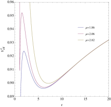
Figure 1: The effective potential $V^{2}_{\rm{eff}}$ of the radial motion is plotted as a function of radial coordinate $r$ for different values of $\mu$ in three ranges, i.e., $\mu=1.86\in(1,2)$, $\mu=2.06\in(2,\sqrt{5})$ and $\mu=2.82\in(\sqrt{5},\infty)$.

According to Eqs.(13,17), the motion equation of a particle reads

$$\dot{r}^{2}=E^{2}-A(r)(1+\frac{L^{2}}{r^{2}}).$$ (21)

By using Eq.(11) and making a change of variable $u^{-1}=r$, we can obtain the orbit motion equation of the test particle

$$(\frac{du}{d\phi})^{2}=\frac{u^{4}}{16}(\frac{E^{2}ab}{L^{2}}-4ab-\frac{a^{2-1/\mu}~{}b^{2+1/\mu}}{L^{2}}),$$ (22)

where $a=2u^{-1}+r_{0}(1-\mu)$ and $b=2u^{-1}+r_{0}(1+\mu)$.

Solving the above motion equation numerically for the three ranges of the parameter $\mu$, we get all types of geodesic orbits in the JNW space-time in detail.

III.1 Case $\mu\in(1,2)$

In Fig.2 the general behavior of the effective potential is shown as a function of the radius with a fixed value of the parameter $\mu=1.86\in(1,2)$ for different values of the angular momentum $L$. The effective potential has a maximum and a minimum which corresponds to the unstable and stable circular orbits, respectively. From the effective potential, we can also expect a bound orbit, a terminating orbit and an escape orbit for the test particle.

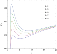
Figure 2: The effective potential $V^{2}_{\rm{eff}}$ of the radial motion is plotted as a function of radial coordinate $r$ for $R_{0}=2,\mu=1.86\in(1,2)$ with different values of $L$.

III.1.1 Time-like circular orbit

In Fig.3, there exist stable and unstable circular orbits. When the energy of the test particle is equal to the peak value of the effective potential curve $E_{c1}$, the test particle will be on an unstable circular orbit, i.e., a tiny perturbation makes the particle fall into the singularity or move on an bound orbit when it fall into the right side of the potential barrier instead; When the energy of the particle is equal to the bottom value $E_{c2}$ of the effective potential, the particle will move on a stable circular orbit.

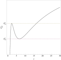
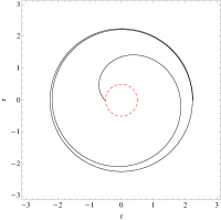
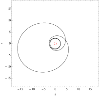
Figure 3: Examples of unstable time-like circular geodesics of JNW space-time with $E_{c1}^{2}=0.925,L=3.6,r_{0}=2,\mu=1.5$.

III.1.2 Time-like bound orbit

The time-like bound orbit for $\mu=1.5\in(1,2)$ is plotted in Fig.4. If the energy of the particle is between the peak value and the bottom value of the potential, the particle will move on a bound orbit with the radius between an aphelion and a perihelion for this case.

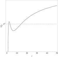
Figure 4: Example of the time-like bound orbit of the JNW space-time with $E^{2}=0.92,L=3.6,r_{0}=2,\mu=1.5$.

III.1.3 Time-like terminating and terminating escape orbits

Fig.5 shows terminating and terminating escape orbits. I) When the energy of the particle is lower than the peak value of effective potential, the particle will move on a terminating orbit from a finite distance on the left side of the potential barrier and end at the singularity eventually; II) When the energy of the particle is higher than the peak value of the potential, The test particle will move on a terminating escape orbit and will end at the singularity if the particle comes from infinity.

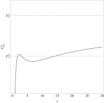
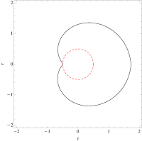
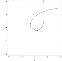
Figure 5: Examples of the time-like terminating and terminating escape orbits of the JNW space-time for $E_{1}^{2}=0.92,E_{2}^{2}=1.05$ with fixed $L=3.6,r_{0}=2,\mu=1.5$.

III.2 Case $\mu\in(2,\sqrt{5})$

In Fig.6 the general behavior of the effective potential is shown as a function of the radius with a fixed value of the parameter $\mu=2.06\in(2,\sqrt{5})$ for different values of the angular momentum $L$. The effective potential has one maximum between two minimums, which correspond to the unstable and stable circular orbits, respectively. There also exists a bound orbit or an escape orbit, but no terminating orbit, i.e., particle will not fall into the singularity.

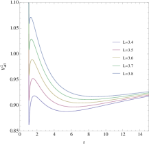
Figure 6: The effective potential $V^{2}_{\rm{eff}}$ of the radial motion is plotted as a function of radial coordinate $r$ for $\mu=2.06\in(2,\sqrt{5})$ for different values of $L$.

III.2.1 Time-like circular orbit

In Fig.7 we can see that there is an unstable circular orbit between two stable circular orbits. I) When the energy of the particle is equal to the bottom values of the effective potential curve $E_{c1}$ or $E_{c2}$, the particle will orbit on two different stable circular orbits. II) When the energy of the particle is equal to the peak value of the potential $E_{c3}$, it will move on an unstable circular orbit. Under this case the test particle will move on two kinds of bound orbits on each side of the potential barrier due to a tiny perturbation.

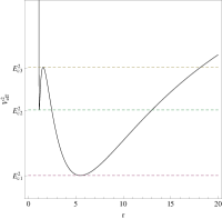
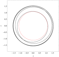
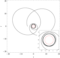
Figure 7: Examples of the time-like unstable circular orbit of the JNW space-time with $E_{c3}^{2}=0.926,L=3.4,r_{0}=2,\mu=2.1$.

III.2.2 Time-like bound orbit

Three kinds of bound orbits are plotted in Fig.8 with the energy levels between the peak value and bottom values or higher than the peak value of the effective potential. The particle will move on the bound orbit between the range of a perihelion and an aphelion and no particle can fall into the singularity.

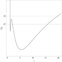
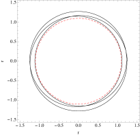
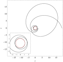
Figure 8: Examples of the time-like bound orbit of the JNW space-time for $E_{1}^{2}=0.92$ and $E_{2}^{2}=0.93$ with fixed $L=3.6,r_{0}=2,\mu=2.1$.

III.2.3 Time-like escape orbit

The time-like escape orbit for $\mu=2.1\in(2,\sqrt{5})$ is plotted in Fig.9, the test particle comes from infinity, then reaches a certain distance which is very close to the singularity, at last is reflected back to infinity.

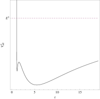
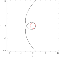
Figure 9: Example of the time-like escape orbit of the JNW space-time with $E^{2}=1,L=3.6,r_{0}=2,\mu=2.1$.

III.3 Case $\mu\in(\sqrt{5},\infty)$

In Fig.10 the general behavior of the effective potential is shown as a function of the radius with a fixed value of the parameter $\mu=2.82\in(\sqrt{5},\infty)$ for different values of the angular momentum $L$. The figure shows that $V^{2}_{\rm{eff}}$ has one minimum which indicates the presence of one region of stable circular orbit. And from the effective potential, we can also find the escape orbit of the test particle in the JNW space-time.

Figure 10: The effective potential $V^{2}_{\rm{eff}}$ of the radial motion is plotted as a function of the radial coordinate $r$ with $\mu=2.82\in(2,\sqrt{5})$ for different values of $L$.

III.3.1 Time-like circular orbit

In Fig.11 when the energy of the particle is equal to the bottom value of the effective potential curve $E_{c}$, the particle will move on a stable circular orbit. There is only one circular orbit for this range of the parameter $\mu$.

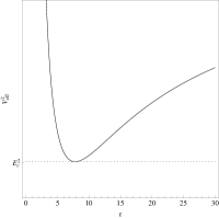
Figure 11: Example of the stable time-like circular geodesics of the JNW space-time with $E_{c}^{2}=0.906,L=3.6,r_{0}=2,\mu=2.8$.

III.3.2 Time-like bound orbit

In Fig.12, the particle will move on a bound orbit with the radius between an aphelion and a perihelion.

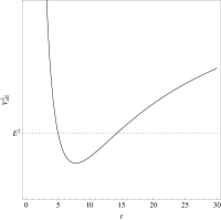
Figure 12: Example of the time-like bound orbit of the JNW space-time with $E^{2}=0.92,L=3.6,r_{0}=2,\mu=2.8$.

III.3.3 Escape orbit

Fig.13 shows two escape orbits corresponding to different energy levels. For these both cases, the particle coming from infinity will reach a certain distance closing to the singularity, then escape to infinity, which is reflected by the potential barrier.

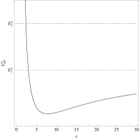
Figure 13: Examples of the time-like escape orbit of the JNW space-time with $E_{1}^{2}=1$ and $E_{2}^{2}=1.1,L=3.6,r_{0}=2,\mu=2.8$.

IV NULL GEODESICS

For the null geodesics $h=0$, the effective potential $V^{2}_{\rm{eff}}$ becomes

$$V_{\rm{eff}}^{2}=A(r)\frac{L^{2}}{B(r)},$$ (23)

for circular geodesics

$$\frac{\partial V}{\partial r}=0,$$ (24)

we have

$$4L(r_{0}-2r)A(r)=0,$$ (25)

where we can see that the null circular geodesics can exist only at the radius $r=\frac{r_{0}}{2}=1$, which is exactly the radius of the photon sphere, i.e. photon moves on a circular trajectory with a fixed radius, which is independent on the parameter $\mu$ and energy level.

Imposing the conditions for the stability of the circular geodesics (16) in Eq.23, we can get

$$8r^{2}-8rr_{0}+r^{2}_{0}(\mu^{2}-2)>0$$ (26)

Solving the above inequality, we find that: I) When $\mu>2$, there is always $\frac{\partial^{2}V}{\partial r^{2}}>0$, and $A(r)>0$, $r>\mu-1>1$, which do not meet the condition for the circular geodesics Eq.(25), so there is no null circular geodesics for $\mu$ at the range of $\mu\in(2,\infty)$; II) When $1<\mu<2$, there exists an unstable circular orbit at the radius $r=1$. The structure of the null geodesics will be different between two distinct ranges of the parameter $\mu$, i.e. $\mu\in(1,2)$ and $\mu\in(2,\infty)$. Fig.14 shows two kinds of effective potentials of the photon. We will discuss all the possible orbits of the photon corresponding to these two cases.

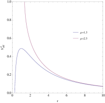
Figure 14: The two cases of effective potential $V^{2}_{\rm{eff}}$ of the radial motion are plotted as a function of the radial coordinate $r$ for $L=3.5,r_{0}=2,\mu=1.3\in(1,2)$ and $\mu=2.3\in(2,\infty)$, which correspond to two kinds of the different null geodesics.

According to Eqs.(13, 23), the motion equation of the photon reads

$$\dot{r}^{2}=E^{2}-A(r)\frac{L^{2}}{r^{2}}.$$ (27)

Using Eq.(11) and making a variable transformation $u^{-1}=r$, Eq. (27) becomes

$$(\frac{du}{d\phi})^{2}=\frac{u^{4}}{16}(\frac{E^{2}a^{2-\frac{2}{\mu}}b^{2+\frac{2}{\mu}}}{L^{2}}-4ab),$$ (28)

where $a=2u^{-1}+r_{0}(1-\mu)$ and $b=2u^{-1}+r_{0}(1+\mu)$.

We solve Eq.(28) numerically to find all types of null geodesics and examine how the parameter $\mu$ influences on the geodesics in the JNW space-time.

IV.1 Case $\mu\in(1,2)$

For this range of the parameter $\mu$, there is only one unstable circular orbit with fixed radius $r=1$. In Fig.15 the general behavior of the effective potential is shown as a function of the radius with a fixed value of the parameter $\mu=1.3\in(1,2)$ for different values of the angular momentum $L$. The effective potential has one maximum at $r=1$ which corresponds to the unstable circular orbit.

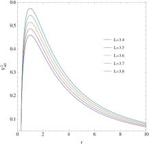
Figure 15: The effective potential $V^{2}_{\rm{eff}}$ of the radial motion is plotted as a function of radial coordinate $r$ with $\mu=1.3\in(1,2)$ for different values of $L$. It is shown in the figure that $V^{2}_{\rm{eff}}$ has one maximum at $r=1$, which indicates the presence of one region of unstable circular orbits.

IV.1.1 Null circular orbit

In Fig.16, from the effective potential we can see that there is only one unstable circular orbit at $r=1$. When the energy of the photo is equal to the peak value $E_{c}$ of the effective potential, the photon is on an unstable circular orbit with radius $r=1$. Any perturbation will make such unstable orbit recede from the circle to the singularity, which is shown in the middle figure of Figs.16, or escape to infinity on the other side of the potential barrier, which is plotted in the right figure of Fig.16.

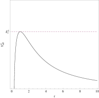
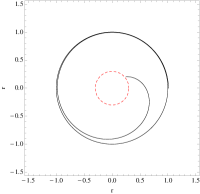
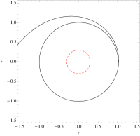
Figure 16: Examples of the unstable null circle geodesics of the JNW space-time with $E^{2}=0.516,L=3.6,r_{0}=2,\mu=1.3$.

IV.1.2 Null terminating escape orbit and terminating orbit

A terminating escape orbit (TEO) in the range $r\in(0,\infty)$ exists, whose minimal radius tends to zero, i.e. the photon comes from infinity and ends at the singularity. So the energy must be higher than the peak value of the barrier; A terminating orbit (TO) is an orbit whose minimal radius tends to zero, that’s to say, the photon comes from a finite distance and ends at the singularity at $r=0$. These two kinds of terminating orbits and the corresponding effective potential are plotted in Fig.17, respectively.

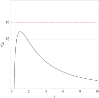
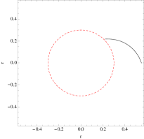
Figure 17: Examples of the null terminating escape orbit, terminating orbit and escape orbit of the JNW space-time with $E_{1}^{2}=0.6,E_{2}^{2}=0.45,L=3.6,r_{0}=2,\mu=1.3$.

IV.1.3 Null escape geodesics

The escape orbit (EO) is an orbit whose minimal radius is not zero, i.e. the photon comes from infinity or a certain distance away from the singularity and then goes back to infinity. In Fig.17, the energy of the photo $E_{1}$ is lower than the peak value of the barrier, the photon is just reflected by the potential barrier.

IV.2 Case $\mu\in(2,\infty)$

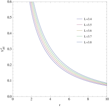
Figure 18: The effective potential $V^{2}_{\rm{eff}}$ of radial motion is plotted as a function of radial coordinate $r$ for different values of $L$, and the example of the null escape geodesics of the JNW space-time with $E^{2}=0.6,L=3.6,r_{0}=2,\mu=2.3$.

In Fig.18 the behavior of the effective potential is shown as a function of the radius with a fixed value of the parameter $\mu=2.3\in(2,\infty)$ for different values of the angular momentum $L$. We can see that $V^{2}_{\rm{eff}}$ does not exist neither any maximum nor minimum, which means that neither unstable circular orbit nor stable circular orbit exists for this range of the parameter $\mu$. From the effective potential we can see that there is only escape orbit for this case. The photon, which comes from infinity, reaches a minimum radius and then goes back to infinity. The photon is just reflected by the potential barrier.

V Summary and Conclusions

In this paper, we have studied the geodesic structure of the JNW space-time which contains a strong curvature naked singularity in detail. We have solved the geodesic equation and analyzed the behavior of effective potential to investigate the motion of massive and massless particles. By using numerical techniques, we have found that for a test particle I) When $\mu\in(1,2)$, there exist stable and unstable circular orbits, a bound orbit, terminating and terminating escape orbits; II) When $\mu\in(2,\sqrt{5})$, there is an unstable circular orbit between two stable circular orbits, or two kinds of bound orbits, or escape orbits; III) When $\mu\in(\sqrt{5},\infty)$, the test particle will move on a stable circular orbit, a abound orbit, or an escape orbit. For a photon, I) When $\mu\in(1,2)$, there are unstable circular orbit, terminating and a terminating escape orbit; II) When $\mu\in(2,\infty)$, there is only an escape orbit.

VI Acknowledgments

S.Z. would like to thank Jiawei Hu for helpful discussions. This project is supported by the National Natural Science Foundation of China under Grant No.10873004, the State Key Development Program for Basic Research Program of China under Grant No.2010CB832803.

References

- Podolsky (1999) J. Podolsky, Gen. Rel. Grav. 31, 1703 (1999).
- Cruz et al. (2005) N. Cruz, M. Olivares, and J. R. Villanueva, Class. Quant. Grav. 22, 1167 (2005).
- Pradhan and Majumdar (2011) P. Pradhan and P. Majumdar, Phys. Lett. A 375, 474 (2011).
- Pugliese et al. (2011a) D. Pugliese, H. Quevedo, and R. Ruffini, Phys. Rev. D 83, 104052 (2011a).
- Pugliese et al. (2013) D. Pugliese, H. Quevedo, and R. Ruffini, arXiv:1304.2940 (2013).
- Pugliese et al. (2011b) D. Pugliese, H. Quevedo, and R. Ruffini, Phys. Rev. D 84, 044030 (2011b).
- Zhou et al. (2011) S. Zhou, J. H. Chen, and Y. J. Wang, Chin. Phys. B 20, 100401 (2011).
- Zhou et al. (2012) S. Zhou, J. H. Chen, and Y. J. Wang, Int. J. Mod. Phys. D 21, 1250077 (2012).
- Joshi et al. (2002) P. S. Joshi, N. Dadhich, and R. Maartens, Phys. Rev. D 65, 101501 (2002).
- Christodoulou (1984) D. Christodoulou, Comm. Math. Phys. 93, 171 (1984).
- Eardley and Smarr (1979) D. M. Eardley and L. Smarr, Phys. Rev. D 19, 2239 (1979).
- Waugh and Lake (1988) B. Waugh and K. Lake, Phys. Rev. D 38, 1315 (1988).
- Goswami and Joshi (2007) R. Goswami and P. S. Joshi, Phys. Rev. D 76, 084026 (2007).
- Harada et al. (1998) T. Harada, H. Iguchi, and K. Nakao, Phys. Rev. D 58, 041502 (1998).
- Joshi and Dwivedi (1993) P. S. Joshi and I. H. Dwivedi, Phys. Rev. D 47, 5357 (1993).
- Ori and Piran (1987) A. Ori and T. Piran, Phys. Rev. Lett. 59, 2137 (1987).
- Lake (1991) K. Lake, Phys. Rev. D 43, 1416 (1991).
- Shapiro and Teukolsky (1991) S. L. Shapiro and S. A. Teukolsky, Phys. Rev. Lett. 66, 994 (1991).
- Stuchlík and Schee (2010) Z. Stuchlík and J. Schee, Class. Quant. Grav. 27, 215017 (2010).
- Virbhadra and Keeton (2008a) K. S. Virbhadra and C. R. Keeton, Phys. Rev. D 77, 124014 (2008a).
- Bambi and Freese (2009) C. Bambi and K. Freese, Phys. Rev. D 79, 043002 (2009).
- Hioki and Maeda (2009) K. Hioki and K. Maeda, Phys. Rev. D 80, 024042 (2009).
- Bambi et al. (2009) C. Bambi, K. Freese, T. Harada, R. Takahashi, and N. Yoshida, Phys. Rev. D 80, 104023 (2009).
- Bambi et al. (2010) C. Bambi, T. Harada, R. Takahashi, and N. Yoshida, Phys. Rev. D 81, 104004 (2010).
- Kovács and Harko (2010) Z. Kovács and T. Harko, Phys. Rev. D 82, 124047 (2010).
- Pugliese et al. (2011c) D. Pugliese, H. Quevedo, and R. Ruffini, Phys. Rev. D 83, 024021 (2011c).
- Janis et al. (1968) A. I. Janis, E. T. Newman, and J. Winicour, Phys. Rev. Lett. 20, 878 (1968).
- Patil and Joshi (2012) M. Patil and P. S. Joshi, Phys. Rev. D 85, 104014 (2012).
- Kovacs and Harko (2010) Z. Kovacs and T. Harko, Phys. Rev. D 82, 124047 (2010).
- Bozza (2002) V. Bozza, Phys. Rev. D 66, 103001 (2002).
- Virbhadra and Ellis (2002) K. S. Virbhadra and G. F. R. Ellis, Phys. Rev. D 65, 103004 (2002).
- Virbhadra and Keeton (2008b) K. Virbhadra and C. Keeton, Phys. Rev. D 77, 124014 (2008b).
- Gyulchev and Yazadjiev (2008) G. N. Gyulchev and S. S. Yazadjiev, Phys. Rev. D 78, 083004 (2008).
- Liao et al. (2014) P. Liao, J. H. Chen, H. Huang, and Y. J. Wang, Gen. Rel. Grav. 46, 1752 (2014).
- Chowdhury et al. (2012) A. N. Chowdhury, M. Patil, D. Malafarina, and P. S. Joshi, Phys. Rev. D 85, 104031 (2012).