Algorithms that satisfy a stopping criterion, probably

Abstract

Iterative numerical algorithms are typically equipped with a stopping criterion, where the iteration process is terminated when some error or misfit measure is deemed to be below a given tolerance. This is a useful setting for comparing algorithm performance, among other purposes.

However, in practical applications a precise value for such a tolerance is rarely known; rather, only some possibly vague idea of the desired quality of the numerical approximation is at hand. We discuss four case studies from different areas of numerical computation, where uncertainty in the error tolerance value and in the stopping criterion is revealed in different ways. This leads us to think of approaches to relax the notion of exactly satisfying a tolerance value.

We then concentrate on a probabilistic relaxation of the given tolerance. This allows, for instance, derivation of proven bounds on the sample size of certain Monte Carlo methods. We describe an algorithm that becomes more efficient in a controlled way as the uncertainty in the tolerance increases, and demonstrate this in the context of some particular applications of inverse problems.

1 Introduction

A typical iterative algorithm in numerical analysis and scientific computing requires a stopping criterion. Such an algorithm involves a sequence of generated iterates or steps, an error tolerance, and a method to compute (or estimate) some quantity related to the error. If this error quantity is below the tolerance then the iterative procedure is stopped and success is declared.

The actual manner in which the error in an iterate is estimated can vary all the way from being rather complex to being as simple as the normed difference between two consecutive iterates. Further, the “tolerance” may actually be a set of values involving combinations of absolute and relative error tolerances. There are several fine points to this, often application-dependent, that are typically incorporated in mathematical software packages (see for instance Matlab’s various packages for solving ordinary differential equation (ODE) or optimization problems). That makes some authors of introductory texts devote significant attention to the issue, while others attempt to ignore it as much as possible (cf. [15, 32, 4]). Let us choose here the middle way of considering a stopping criterion in a general form

$${\rm error\_estimate}(k)\leq\rho,$$ (1)

where $k$ is the iteration or step counter, and $\rho>0$ is the tolerance, assumed given.

But now we ask, is $\rho$ really given?! Related to this, we can also ask, to what extent is the stoppping criterion adequate?

• The numerical analyst would certainly like $\rho$ to be given. That is because their job is to invent new algorithms, prove various assertions regarding convergence, stability, efficiency, and so on, and compare the new algorithm to other known ones for a similar task. For the latter aspect, a rigid deterministic tolerance for a trustworthy error estimate is indispensable.

  Indeed, in research areas such as image processing where criteria of the form (1) do not seem to capture certain essential features and the “eye norm” rules, a good comparison between competing algorithms can be far more delicate. Moreover, accurate comparisons of algorithms that require stochastic input can be tricky in terms of reproducing claimed experimental results.

• On the other hand, a practitioner who is the customer of numerical algorithms, applying them in the context of some complicated practical application that needs to be solved, will more often than not find it very hard to justify a particular choice of a precise value for $\rho$ in (1).

Our first task in what follows is to convince the reader that often in practice there is a significant uncertainty in the actual selection of a meaningful value for the error tolerance $\rho$, a value that must be satisfied. Furthermore, numerical analysts are also subconsciously aware of this fact of life, even though in most numerical analysis papers such a value is simply given, if at all, in the numerical examples section. Four typical yet different classes of problems and methods are considered in Section 2.

Once we are all convinced that there is usually a considerable uncertainty in the value of $\rho$ (hence, we only know it “probably”), the next question is what to do with this notion. The answer varies, depending on the particular application and the situation at hand. In some cases, such as that of Section 2.1, the effective advice is to be more cautious, as mishaps can happen. In others, such as that of Section 2.2, we are simply led to acknowledge that the value of $\rho$ may come from thin air (though one then concentrates on other aspects). But there are yet other classes of applications and algorithms, such as in Sections 2.3 and 2.4, for which it makes sense to attempt to quantify the uncertainty in the error tolerance $\rho$ using a probabilistic framework. We are not proposing in this article to propagate an entire probability distribution for $\rho$: that would be excessive in most situations. But we do show, by studying an instance extended to a wide class of problems, that employing such a framework can be practical and profitable.

Following Section 2.4 we therefore consider in Section 3 a particular manner of relaxing the notion of a deterministic error tolerance, by allowing an estimate such as (1) to hold only within some given probability. Relaxing the notion of an error tolerance in such a way allows the development of theory towards an uncertainty quantification of Monte Carlo methods (e.g., [1, 8, 53, 37, 35]). We concentreate on the problem of estimating the trace of symmetric positive semi-definite (SPSD) matrices that are given implicitly, i.e., as a routine to compute their product with any vector of suitable size. We then use this to satisfy in a probabilistic sense an error tolerance for approximating a data misfit function for cases where many data sets are given. Some details of results of this type that are relevant in the present context and have been proved in [46, 47] are provided.

In Section 4 we apply the results of Section 3 to form a randomized algorithm for approximately solving inverse problems involving partial differential equation (PDE) systems. We concentrate on cases where many data sets are provided (which is typical in several important applications) that correspondingly require the solution of many PDEs. Conclusions and some additional general comments are offered in Section 5.

While this article concentrates on bringing to the fore a novel point of view, we also note that the observations in Section 2.2.1, and to a lesser extent also Section 2.3.1, are novel. The results displayed in Figures 1 and 3 are new.

2 Case studies

In this section we consider four classes of problems and associated algorithms, in an attempt to highlight the use of different tests of the form (1) and in particular the implied level of uncertainty in the choice of $\rho$.

2.1 Stopping criterion in initial value ODE solvers

Using a case study, we show in this section that numerical analysts, too, can be quick to not consider $\rho$ as a “holy constant”: we adapt to weaker conditions in different ways, depending on the situation and the advantage to be gained in relaxing the notion of an error tolerance.

Let us consider an initial value ODE system in “time” $t$, written as

$$\frac{d{\bf u}}{dt} = {\bf f}(t,{\bf u}),\quad 0\leq t\leq b,$$ (2a)

$${\bf u}(0) = {\bf v}_{0},$$ (2b)

with ${\bf v}_{0}$ a given initial value vector. A typical adaptive algorithm proceeds to generate pairs $(t_{i},{\bf v}_{i}),\ i=0,1,2,\ldots,N$, in $N$ consecutive steps, thus forming a mesh $\pi$ such that

$$\pi:0=t_{0}<t_{1}<\cdots<t_{N-1}<t_{N}=b,$$

and ${\bf v}_{i}\approx{\bf u}(t_{i}),\ i=1,\ldots,N$.

Denoting the numerical solution on the mesh $\pi$ by ${\bf v}^{\pi}$, and the restriction of the exact ODE solution to this mesh by ${\bf u}^{\pi}$, there are two general approaches for controling the error in such an approximation.

• Given a tolerance value $\rho$, keep estimating the global error and refining the mesh (i.e., the gamut of step sizes) until roughly

  $$\|{\bf v}^{\pi}-{\bf u}^{\pi}\|_{\infty}\leq\rho.$$ (3)

  Details of such methods can be found, for instance, in [29, 34, 13, 6].

  In (3) we could replace the absolute tolerance by a combination of absolute and relative tolerances, perhaps even different ones for different ODE equations. But that aspect is not what we concentrate on in this article.

• However, most general-purpose ODE codes estimate a local error measure for (1) instead, and refine the step size locally. Such a procedure advances one step at a time, and estimates the next step size using local information related to the local truncation error, or simply the difference between two approximate solutions for the next time level, one of which presumed to be significantly more accurate than the other. For details see [29, 30, 6] and many references therein. In particular, the popular Matlab codes ode45 and ode23s use such a local error control.

The reason for employing local error control is that this allows for developing a much cheaper and yet more sensitive adaptive procedure, an advantage that cannot be had, for instance, for general boundary value ODE problems; see, e.g., [5].

But does this always produce sensible results?! The answer to this question is negative. A simple example to the contrary is the problem

$$\frac{du}{dt}=100(u-\sin t)+\cos t,\quad u(0)=0,~{}b=1.$$

Local truncation (or discretization) errors for this unstable initial value ODE propagate like $\exp(100t)$, a fact that is not reflected in the local behaviour of the exact solution $u(t)=\sin t$ on which the local error control is based. Thus, we may have a large error $\|{\bf v}^{\pi}-{\bf u}^{\pi}\|_{\infty}$ even if the local error estimate is bounded by $\rho$ for a small value of $\rho$.

2.1.1 Local error control can be dangerous even for a stable ODE system

Still one can ask, are we safe with local error control in case that we know that our ODE problem is stable? Here, by “safe” we mean that the global error will not be much larger than the local truncation error in scaled form. The answer to this more subtle question turns out to be negative as well. The essential point is that the global error consists of an accumulation of contributions of local errors from previous time steps. If the ODE problem is asymptotically stable (typically, because it describes a damped motion) then local error contributions die away as time increases, often exponentially fast, so at some fixed time only the most recent local error contributions dominate in the sum of contributions that forms the global error. However, if the initial value ODE problem is merely marginally stable (which is the case for Hamiltonian systems) then local error contributions propagate undamped, and their accumulation over many time steps can therefore be significantly larger than just one or a few such errors.

For a simple concrete example, consider applying ode45 with default tolerances to find the linear oscillator with a slowly varying frequency that satisfies the following initial value ODE for $p(t)$:

$$\frac{dq}{dt} = \lambda^{2}p,\quad q(0)=1,$$

$$\frac{dp}{dt} = -(1+t)^{2}q,\quad p(0)=0.$$

Here $\lambda>0$ is a given parameter. Thus, ${\bf u}=(q,p)^{T}$ in the notation of (2). This is a Hamiltonian system, with the Hamiltonian function given by

$$H(q,p,t)=\frac{1}{2}\left[((1+t)q)^{2}+(\lambda p)^{2}\right].$$

Now, since the ODE is not autonomous, the Hamiltonian is not constant in time. However, the adiabatic invariant

$$J(q,p,t)=H(q,p,t)/(1+t)$$

(see, e.g., [39, 7]) is almost constant for large $\lambda$, satisfying

$$[J(t)-J(0)]/J(0)={\mathcal{O}}(\lambda^{-1})$$

over the interval $[0,1]$. This condition means in particular that for $\lambda\gg 1$ and the initial values given above, $J(1)=J(0)+{\mathcal{O}}(\lambda^{-1})\approx J(0)$.

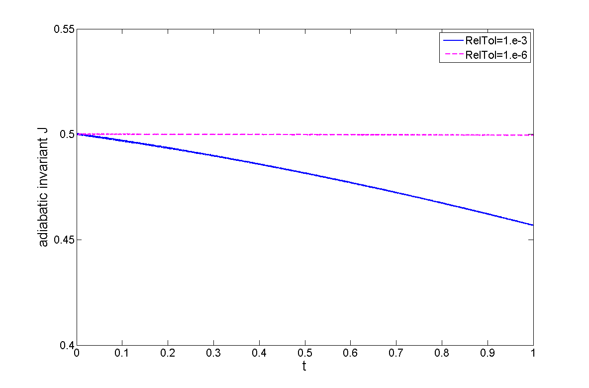
Figure 1: Adiabatic invariant approximations obtained using Matlab’s package ode45 with default tolerances (solid blue) and stricter tolerances (dashed magenta).

Figure 1 depicts two curves approximating the adiabatic invariant for $\lambda=1000$. Displayed are the calculated curve using ode45 with default tolerances (absolute=1.e-6, relative=1.e-3), as well as what is obtained upon using ode45 with the stricter relative tolerance RelTol=1.e-6. From the figure it is clear that when using the looser tolerance, the resulting approximation for $J(1)$ differs from $J(0)$ by far more than what $\lambda^{-1}=$1.e-3 and RelTol=1.e-3 would indicate, while the stricter tolerance gives a qualitatively correct result, using the “eye norm”. Annoyingly, the qualitatively incorrect result does not look like “noise”: while not being physical, it looks downright plausible, and hence could be misleading for an unsuspecting user. Adding to the pain is the fact that this occurs for default tolerance values, an option that a vast majority of users would automatically select. $\blacklozenge$

A similar observation holds when trying to approximate the phase portrait or other properties of an autonomous Hamiltonian ODE system over a long time interval using ode45 with default tolerances: this may produce qualitatively wrong results. See for instance Figures 16.12 and 16.13 in [4]: the Fermi-Pasta-Ulam problem solved there is described in detail in Chapter 1 of [28]. What we have just shown here is that the phenomenon can arise also for a very modest system of two linear ODEs that do not satisfy any exact invariant.

We hasten to add that the documentation of ode45 (or other such codes) does not propose to deliver anything like (3). Rather, the tolerance is just a sort of a knob that is turned to control local error size. However, this does not explain the popularity of such codes despite their limited offers of assurance in terms of qualitatively correct results.

Our key point in the present section is the following: we propose that one reason for the popularity of ODE codes that use only local error control is that in applications one rarely knows a precise value for $\rho$ as used in (3) anyway. (Conversely, if such a global error tolerance value is known and is important then codes employing a global error control, and not ode45, should be used.) Opting for local error control over global error control can therefore be seen as one specific way of adjusting mathematical software in a deterministic sense to realistic uncertainties regarding the desired accuracy.

2.2 Stopping criterion in iterative methods for linear systems

In this case study, extending basic textbook material, we argue not only that tolerance values used by numerical analysts are often determined solely for the purpose of the comparison of methods (rather than arising from an actual application), but also that this can have unexpected effects on such comparisons. In Section 2.2.1 we further make some novel, and we think intriguing, observations on PDE discretizations, which arise in the present context although having little to do with our main theme.

Consider the problem of finding ${\bf u}$ satisfying

$$A{\bf u}={\bf b},$$ (4)

where $A$ is a given $s\times s$ symmetric positive definite matrix such that one can efficiently carry out matrix-vector products $A{\bf v}$ for any suitable vector ${\bf v}$, but decomposing the matrix directly (and occasionally, even looking at its elements) is too inefficient and as such is “prohibited”. We relate to such a matrix as being given implicitly. The right hand side vector ${\bf b}$ is given as well.

An iterative method for solving (4) generates a sequence of iterates ${\bf u}_{1},{\bf u}_{2},\ldots,{\bf u}_{k},\ldots$ for a given initial guess ${\bf u}_{0}$. Denote by ${\bf r}_{k}={\bf b}-A{\bf u}_{k}$ the residual in the $k$th iterate. The MINRES method, or its simpler version Orthomin(2), can be applied to reduce the residual norm so that

$$\|{\bf r}_{k}\|_{2}\leq\rho\|{\bf r}_{0}\|_{2}$$ (5)

in a number of iterations $k$ that in general is at worst $\mathcal{O}\left(\sqrt{\kappa(A)}\right)$, where $\kappa(A)=\|A\|_{2}\|A^{-1}\|_{2}$ is the condition number of the matrix $A$. Below in Table 1 we refer to this method as MR. The more popular conjugate gradient (CG) method generally performs comparably in practice. We refer to [24] for the precise statements of convergence bounds and their proofs.

A well-known and simpler-looking family of gradient descent methods is given by

$${\bf u}_{k+1}={\bf u}_{k}+\alpha_{k}{\bf r}_{k},$$ (6)

where the scalar $\alpha_{k}>0$ is the step size. Such methods have recently come under intense scrutiny because of applications in stochastic programming and sparse solution recovery. Thus, it makes sense to evaluate and understand them in the simplest context of (4), even though it is commonly agreed that for the strict purpose of solving (4) iteratively, CG cannot be significantly beaten. Note that (6) can be viewed as a forward Euler discretization of the artificial time ODE

$$\frac{d{\bf u}}{dt}=-A{\bf u}+{\bf b},$$ (7)

with “time” step size $\alpha_{k}$. Next we consider two choices of this step size.

The steepest descent (SD) variant of (6) is obtained by the greedy (exact) line search for the function

$$f({\bf u})=\frac{1}{2}{\bf u}^{T}A{\bf u}-{\bf b}^{T}{\bf u},$$

which gives

$$\alpha_{k}=\alpha_{k}^{SD}=\frac{{\bf r}_{k}^{T}{\bf r}_{k}}{{\bf r}_{k}^{T}A{\bf r}_{k}}\equiv\frac{({\bf r}_{k},{\bf r}_{k})}{({\bf r}_{k},A{\bf r}_{k})}\equiv\frac{\|{\bf r}_{k}\|_{2}^{2}}{\|{\bf r}_{k}\|_{A}^{2}}.$$

However, SD is very slow, requiring $k$ in (5) to be proportional to $\kappa(A)$; see, e.g., [2].

A more enigmatic choice in (6) is the lagged steepest descent (LSD) step size

$$\alpha_{k}=\alpha_{k}^{LSD}=\frac{({\bf r}_{k-1},{\bf r}_{k-1})}{({\bf r}_{k-1},A{\bf r}_{k-1})}.$$

It was first proposed in [9] and practically used for instance in [10, 16]. To the best of our knowledge, there is no known a priori bound on how many iterations as a function of $\kappa(A)$ are required to satisfy (5) with this method [9, 44, 22, 17].

We next compare these four methods in a typical fashion for a prototypical PDE example, where we consider the model Poisson problem

$$-\Delta u=1,\quad 0<x,y<1,$$

subject to homogeneous Dirichlet BC, and discretized by the usual 5-point difference scheme on a $\sqrt{s}\times\sqrt{s}$ uniform mesh. Denote the reshaped vector of mesh unknowns by ${\bf u}\in{\rm I\!R}^{s}$. The largest eigenvalue of the resulting matrix $A$ in (4) is $\lambda_{\max}=4h^{-2}(1+\cos(\pi h))$, and the smallest is $\lambda_{\min}=4h^{-2}(1-\cos(\pi h))$, where $h=1/(\sqrt{s}+1)$. Hence by Taylor expansion of $\cos(\pi h)$, for $h\ll 1$ the condition number is essentially proportional to $s$:

$$\kappa(A)=\frac{\lambda_{\max}}{\lambda_{\min}}\approx\left(\frac{2}{\pi}\right)^{2}s.$$

In Table 1 we list iteration counts required to satisfy (5) with $\rho=10^{-7}$, starting with ${\bf u}_{0}={\bf 0}$.

$s$	MR	CG	SD	LSD
$7^{2}$	9	9	196	45
$15^{2}$	26	26	820	91
$31^{2}$	54	55	3,337	261
$63^{2}$	107	109	13,427	632
$127^{2}$	212	216	53,800	1,249

Table 1: Iteration counts required to satisfy (5) for the Poisson problem with tolerance $\rho=10^{-7}$ and different mesh sizes $s$.

But now, returning to the topic of the present article, we ask, why insist on $\rho=10^{-7}$? Indeed, the usual observation that one draws from the columns of values for MR, CG and SD in a table such as Table 1, is that the first two grow like $\sqrt{\kappa(A)}\propto\sqrt{s}$ while the latter grows like $\kappa(A)\propto s$. The value of $\rho$, so long as it is not too large, does not matter at all!

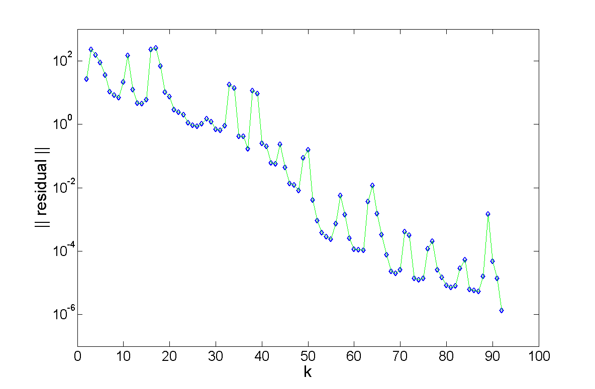
(a) Residuals

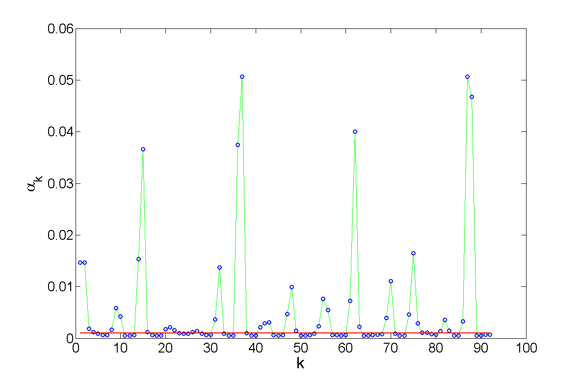
(b) Step sizes

Figure 2: Relative residuals and step sizes for solving the model Poisson problem using LSD on a $15\times 15$ mesh. The red line in (b) is the forward Euler stability limit.

And yet, this is not quite the case for the LSD iteration counts. These do not decrease in the same orderly fashion as the others, even though they are far better (in the sense of being significantly smaller) than those for SD. Indeed, this method is chaotic [17], and the residual norm decreases rather non-monotonically, see Figure 2(a). Thus, the iteration counts in Table 1 correspond to the iteration number $k=k^{*}$ where the rough-looking relative residual norm first records a value below the tolerance $\rho$. Unlike the other three methods, here the particular value of the tolerance, picked just to be concrete, does play an unwanted role in the relative values, as a function of $s$, or $\kappa(A)$, of the listed iteration counts. $\blacklozenge$

2.2.1 How large can the step size be? – benefitting from a discretize-first approach

While on the subject of LSD, let us also remark that gradient descent for this example can be viewed as an application of the forward Euler method via (7) to find the steady state of the heat equation

$$\frac{\partial u}{\partial t}=\Delta u+1.$$ (8)

(Homogeneous Dirichlet boundary conditions for all $t>0$ are assumed already incorporated into the Poisson-Laplace operator $\Delta$.)

The forward Euler time-stepping method with step size $\alpha$, applied as a semi-discretization in time to this PDE problem, reads

$$u_{k+1}=u_{k}+\alpha(\Delta u_{k}+1),$$ (9)

where $u_{k}=u_{k}(x,y)$. However, this cannot be stable for any $\alpha>0$. To see this, think of what happens to a discontinuous initial condition function $u_{0}(x,y)$ when its spatial derivatives are repeatedly taken as in (9).

Next, let us discretize in space first, obtaining (7), and follow this with a forward Euler discretization in time (i.e., apply gradient descent (6)). It is well-known that if the step size $\alpha_{k}=\alpha$ is constant for all $k$ then stability requires the restriction $\alpha\leq.25/s$. In fact, the precise stability statement is $\alpha\leq 2/\lambda_{\max}$, where $\lambda_{\max}$ is the largest eigenvalue of the matrix $A$ given above. This restriction becomes more severe as $s$ grows, and in the limit $s\rightarrow\infty$ we obtain the unconditionally unstable method (9).

So far, things are as expected. But now, if $\alpha_{k}$ is allowed to vary with $k$ then no such stability requirement holds for all $k$! Indeed, if $\alpha_{k}=1/\lambda_{\min}$ then although this does enlarge the magnitude of high-frequency components in the residual (we are using multigrid jargon here; see [51]), it may decrease low frequency ones rapidly. The temporary increase in high frequency component magnitudes can then be alleviated by next taking a few small step sizes which are known to be particularly efficient in reducing those high frequency amplitudes. Next we observe that as the uniform mesh size $s$ grows, $\lambda_{\min}\rightarrow 2\pi$, which is independent of the discretization mesh width. So this large step size is in effect constant as the mesh is refined, and yet the method can be convergent. This argument follows from a discretize-first approach, and cannot be seen from (9).

Returning to LSD as a method for automatically choosing the step sizes in the forward Euler method, the results are recorded in Figure 2(b). In fact, in this particular example we find upon decreasing the spatial mesh width that $\max_{k}\alpha_{k}\approx.05$, independently of $s$. Thus, what was merely possible in the previous paragraph is in fact automatically achieved by an LSD method that provably converges to steady state.

To the best of our knowledge, this result is novel, and moreover we have found that it is unintuitive to many experts in numerical PDEs. Hence we chose to incorporate it in this article, despite the fact that it does not directly relate to its main theme.

2.3 Data fitting and inverse problems

In the previous two case studies we have encountered situations where the intuitive use of an error tolerance within a stopping criterion could differ widely (and wildly) from the notion that is embodied in (1) for the consumer of numerical analysts’ products. We next consider a family of problems where the value of $\rho$ in a particular criterion (1) is more directly relevant.

Suppose we are given observed data ${\bf d}\in{{\rm I\!R}}^{l}$ and a forward operator $f_{i}(m),\ i=1,\ldots,l$, which provides predicted data for each instance of a distributed parameter function $m$. The (unknown) function $m$ is defined in some domain $\Omega$ in physical space and possibly time. We are particularly interested here in problems where $f$ involves the solution $u$ in $\Omega$ of some linear PDE system, sampled in some way at the points where the observed data are provided. Further, for a given mesh $\pi$ discretizing $\Omega$, we consider a corresponding discretization (i.e., nodal representation) of $m$ and $u$, as well as the differential operator. Reshaping these mesh functions into vectors we can write the resulting approximation of the forward operator as

$${\bf f}({\bf m})=P{\bf u}=PG({\bf m}){\bf q},$$ (10)

where the right hand side vector ${\bf q}$ is commonly referred to as a source, $G$ is a discrete Green’s function (i.e., the inverse of the discretized PDE operator), ${\bf u}=G({\bf m}){\bf q}$ is the field (i.e., the PDE solution, here an interim quantity), and $P$ is a projection matrix that projects the field to the locations where the data values ${\bf d}$ are given.

This setup is typical in the thriving research area of inverse problems; see, e.g., [20, 52]. A specific example is provided in Section 4.

The inverse problem is to find ${\bf m}$ such that the predicted and observed data agree to within noise ${\bm{\eta}}$: ideally,

$${\bf d}={\bf f}({\bf m})+{\bm{\eta}}.$$ (11)

To obtain such a model ${\bf m}$ that satisfies (11) we need to estimate the misfit function $\phi({\bf m})$, i.e., the normed difference between observed data ${\bf d}$ and predicted data ${\bf f}({\bf m})$. An iterative algorithm is then designed to sufficiently reduce this misfit function. But, which norm should we use to define the misfit function?

It is customary to conveniently assume that the noise satisfies ${\bm{\eta}}\sim\mathcal{N}(0,\sigma I)$, i.e., that the noise is normally distributed with a scaled identity for the covariance matrix, where $\sigma$ is the standard deviation. Then the maximum likelihood (ML) data misfit function is simply the squared $\ell_{2}$-norm

$$\phi({\bf m})=\|{\bf f}({\bf m})-{\bf d}\|_{2}^{2}.$$ (12)

In this case, the celebrated Morozov discrepancy principle yields the stopping criterion

$$\phi({\bf m})\leq\rho,\quad{\rm where~{}}\rho=\sigma^{2}l,$$ (13)

see, e.g., [20, 40, 38]. So, here is a class of problems where we do have a meaningful and directly usable tolerance value!

Assuming that a known tolerance $\rho$ must be satisfied as in (13) is often too rigid in practice, because realistic data do not quite satisfy the assumptions that have led to (13) and (12). Well-known techniques such as L-curve and GCV (see, e.g., [52]) are specifically designed to handle more general and practical cases where (13) cannot be used or justified. Also, if (13) is used then a typical algorithm would try to find ${\bf m}$ such that $\phi({\bf m})$ is (smaller but) not much smaller than $\rho$, because having $\phi({\bf m})$ too small would correspond to fitting the noise – an effect one wants to avoid. The latter argument and practice do not follow from (13).

Moreover, keeping the misfit function $\phi({\bf m})$ in check does not necessarily imply a quality reconstruction (i.e., an acceptable approximation ${\bf m}$ for the “true solution” ${\bf m}_{\rm true}$, which can be an elusive notion in itself). However, $\phi({\bf m})$, and not direct approximations of $\|{\bf m}_{\rm true}-{\bf m}\|$, is what one typically has to work with. So any additional a priori information is often incorporated through some regularization.

Still, despite all the cautious comments in the preceding two paragraphs, we have in (13) in a sense a more meaningful practical expression for stopping an iterative algorithm than hitherto.

2.3.1 Regularization and constrained formulations

Typically there is a need to regularize the inverse problem, and often this is done by adding a regularization term to (12). Thus, one attempts to approximately solve the Tikhonov-type problem

$$\min_{{\bf m}}~{}\phi({\bf m})+\lambda R({\bf m}),$$ (14)

where $R({\bf m})\geq 0$ is a prior (we are thinking of some norm or semi-norm of ${\bf m}$), and $\lambda\geq 0$ is a regularization parameter. Two other forms of the same problem (14) immediately arise upon interpreting $\lambda$ or $\lambda^{-1}$ as a Lagrange multiplier. These are the constrained optimization formulations

$$\min_{\bf m}~{}\phi({\bf m}),\quad{\rm s.t.~{}}R({\bf m})\leq\tau;\ \ {\rm and}$$ (15)

$$\min_{\bf m}~{}R({\bf m}),\quad{\rm s.t.~{}}\phi({\bf m})\leq\rho.$$ (16)

The non-negative parameters $\rho,\ \tau$ and $\lambda$ are related to one another in a nontrivial manner that makes these three formulations indeed equivalent; see, e.g., [10].

Each of these formulations has its fan club. The inevitable discussion regarding which is best becomes more heated when $R$ involves the $\ell_{1}$-norm, corresponding to a prior that favours some form of sparsity; see [18] and references therein. This is so not only because sparsity is popular and extremely useful, but also because use of the $\ell_{1}$-norm introduces lower smoothness in $R({\bf m})$. In such circumstances, the formulation (15) can be more directly amenable to efficient solution techniques (see the equivocal [10]), while (16) has the advantage that the tolerance $\rho$ is known (cf. (13)) with far less a priori uncertainty than $\tau$ or $\lambda$. Thus, the popular question of choosing the most practically advantageous formulation from among (14)–(16) (see, e.g., [31]) is tied to the topic of the present article.

2.4 Least squares data fitting with many data sets

In our fourth case study we generalize the setting of Section 2.3, allowing not only one but several (indeed, many) data sets ${\bf d}_{i},\ i=1,\ldots,s$, where each data set has length $l$, so ${\bf d}_{i}\in{{\rm I\!R}}^{l}$. Unless $s$ is small, working with such a problem can be prohibitively expensive, so we next use randomized approximations to the misfit function. This in turn provides a new meaning to the uncertainty in the given tolerance $\rho$, which we further explore in later sections.

We can conveniently define an $l\times s$ data matrix $D$ whose $i$th column is ${\bf d}_{i}$. Correspondingly, there are forward operators

$${\bf f}_{i}({\bf m}) \equiv {\bf f}({\bf m},{\bf q}_{i})=PG({\bf m}){\bf q}_{i},\quad i=1,\ldots,s,$$ (17a)

where $${\bf q}_{i} l\times s F({\bf m}) {\bf f}_{i} i {\bf m}$$ are different sources, and we arrange the forward operator in form of an matrix function which has as its th column. The inverse problem is to find such that the predicted and observed data agree to within noise,

$${\bf d}_{i}={\bf f}_{i}({\bf m})+{\bm{\eta}}_{i},\quad i=1,2,\ldots,s.$$ (17b)

Assuming next that $${\bm{\eta}}_{i}\sim\mathcal{N}(0,\sigma I)$$, the ML data misfit function is

$$\phi({\bf m})=\sum_{i=1}^{s}\|{\bf f}_{i}({\bf m})-{\bf d}_{i}\|_{2}^{2}=\|F({\bf m})-D\|_{F}^{2},$$ (17c)

where the subscript $$F$$ denotes the Frobenius norm. In this case, the discrepancy principle yields the stopping criterion

$$\phi({\bf m})\leq\rho,\quad{\rm where~{}}\rho=\sigma^{2}ls.$$ (17d)

So, as in Section 2.3, provided that all assumptions hold we have a decent idea of a stopping tolerance value for an iterative method that generates iterates $${\bf m}_{k},k=1,2,\ldots \phi$$, in an attempt to decrease until (17d) holds with approximate equality.

However, when $s$ is very large, since $s$ evaluations of $G({\bf m}){\bf q}_{i}$ are required just to form $F({\bf m})$ for a given ${\bf m}$, we obtain an instance where the matrix $B=F({\bf m})-D$ can be prohibitively expensive to calculate explicitly (Section 4 provides a concrete example). Hence the matrix $A=B^{T}B$ is implicit symmetric positive semi-definite (SPSD) (cf. Section 2.2). Furthermore, we have

$$\phi({\bf m})=\|B\|_{F}^{2}=tr(A)={\mathbb{E}}(\|B{\bf w}\|_{2}^{2}),$$ (18)

where $tr(A)$ denotes the trace of the matrix $A$, ${\mathbb{E}}$ stands for expectation, and ${\bf w}$ stands for a random vector drawn from any distribution satisfying ${\mathbb{E}}({\bf w}{\bf w}^{T})=\mathbb{I}$.

Inexpensive approximate alternatives to working with all $s$ data sets throughout an algorithm for finding a suitable ${\bf m}$ may be obtained by approximating the misfit function $\phi({\bf m})$ in (17c). Specifically, the rightmost expression in (18) suggests a Monte Carlo sampling method, obtaining

$$\widehat{\phi}({\bf m},n)\mathrel{\mathop{:}}=\frac{1}{n}\sum_{j=1}^{n}\|B({\bf m}){\bf w}_{j}\|_{2}^{2}\approx\phi({\bf m}).$$ (19)

Note that $\widehat{\phi}({\bf m},n)$ is an unbiased estimator of $\phi({\bf m})$, as we have $\phi({\bf m})={\mathbb{E}}(\widehat{\phi}({\bf m},n))$. For the forward operators (17a), if $n\ll s$ (in words, the sample size $n$ is much smaller than the total number of data sets $s$) then this procedure yields a very efficient algorithm for approximating the misfit (17c). This is so because

$$\sum_{i=1}^{s}{\bf f}({\bf m},{\bf q}_{i})w_{i}={\bf f}({\bf m},\sum_{i=1}^{s}w_{i}{\bf q}_{i}),$$

which can be computed with a single evaluation of ${\bf f}$ per realization of the random vector ${\bf w}=(w_{1},\ldots,w_{s})^{T}$, so in total $n$ (rather than $s$) such evaluations are required [26, 48]. An example utilizing (19) is considered in Section 4 below.

But now it is natural to ask, how large should $n$ be? Generally speaking, the larger $n$ is, the closer $\widehat{\phi}({\bf m},n)$ is to $\phi({\bf m})$. So we are led to ask how important it is to pedantically satisfy (17d). This in turn brings up the question that is the common refrain of this section, namely, the extent to which the stopping criterion is really known and as such must be obeyed. Here, a higher uncertainty in $\rho$ and (17) allows a more efficient solution algorithm because a smaller $n$ will suffice. In the context of the present randomized algorithm it is therefore natural to consider satisfying the error criterion (1) only within some probability range. To concentrate on this aspect we isolate it by assuming that $\rho$ in (17d) is given and the error model that enables this is approximately valid.

3 Probabilistic relaxation of a stopping criterion

The previous section details four different case studies which highlight the fact of life that in applications an error tolerance for stopping an algorithm is rarely known with absolute certainty. Thus, we can say that such a tolerance is only “probably” known. Yet in some situations, it is also possible to assign it a more precise meaning in terms of statistical probability. This holds true for the case study in Section 2.4, with which we proceed below. Thus, in the present section we consider a way to relax (1), which is more systematic and also allows for further theoretical developments. Specifically, we consider satisfying a tolerance in a probabilistic sense.

Suppose we seek an unbiased estimator $\hat{g}(x)$ to a real valued function $g(x)$ (so ${\mathbb{E}}(\hat{g}(x))=g(x)$, where $\mathbb{E}$ denotes expectation). Then, given a pair of values $(\varepsilon,\delta)$, both small and positive, we require

$$Pr\big{(}|\hat{g}(x)-g(x)|\leq\varepsilon~{}|g(x)|\big{)}\geq 1-\delta.$$ (20)

The parameters $\varepsilon$ and $\delta$ relate to the relative accuracy and the probabilistic guarantee of such an estimation, respectively [1]. In Section 3.1 we consider applying this notion to the problem of trace estimation. Then in Section 3.2 we apply the results of Section 3.1 to the case study of Section 2.4. The uncertainty in the stopping tolerance $\rho$ is quantified in terms of parameters $\varepsilon$ and $\delta$ towards the end of this section.

3.1 Estimating the trace of an implicit matrix

As in Section 2.2 we consider an $s\times s$ matrix $A$ that is given only implicitly, through matrix-vector products. We assume that $A=B^{T}B$, where $B$ is some real rectangular matrix with $s$ columns, and wish to approximate the trace, $tr(A)=\sum_{i=1}^{s}a_{i,i}$, without having the luxury of knowing the diagonal elements $a_{i,i}$. This task has several applications; see [8, 46]. We consider it here mainly as a preparatory step, given the appearance of the trace in (18).

Note that if ${\bf x}$ is the $i$th column of the $s\times s$ identity matrix then $({\bf x},A{\bf x})=a_{i,i}$. Hence, $tr(A)$ can be calculated in $s$ matrix-vector products. However, $s$ is very large so we want a cheaper approximation. Towards that goal, observe that if ${\bf w}$ stands for a random vector drawn from a probability distribution ${\cal D}$ satisfying $\mathbb{E}[{\bf w}{\bf w}^{T}]=I$, then

$$tr(A)={\mathbb{E}}[({\bf w},A{\bf w})].$$ (21)

So, we consider the Monte Carlo approximation $tr(A)\approx tr_{\cal D}(A)$, defined by

$$tr_{\cal D}(A)\mathrel{\mathop{:}}=\frac{1}{n}\sum_{i=1}^{n}({\bf w}_{i},A{\bf w}_{i})=\frac{1}{n}\sum_{i=1}^{n}\|B{\bf w}_{i}\|_{2}^{2}\ ,$$ (22)

where ${\bf w}_{i}$ are drawn from the distribution ${\cal D}$, and hopefully $n\ll s$.

The next question is, how small can we take $n$ to be? In other words, how can we quantify the uncertainty in such an approximation? Here is where the pair $(\varepsilon,\delta)$ appearing in (20) comes in handy for deriving probabilistic necessary and sufficient conditions on the size of $n$. Below we state two results that were proved in [46, 47].

Let us restate (20) in the present context as

$$Pr\big{(}|tr_{\cal D}(A)-tr(A)|\leq\varepsilon~{}|tr(A)|\big{)}\geq 1-\delta.$$ (23)

Further, given the pair $(\varepsilon,\delta)$ (both values positive and small), define the constant

$$c=c(\varepsilon,\delta)=\varepsilon^{-2}\ln(2/\delta).$$ (24)

This constant appears in all estimates of the type stated in Theorem 1 below. Note its strong dependence on $\varepsilon$ and much weaker dependence on $\delta$, in the sense of how rapidly $c$ grows as these values shrink.

Theorem 1

• Let ${\cal D}$ be the Gaussian (i.e., standard normal) probability distribution. Then the probabilistic bound (23) holds if

  $$n\geq 8c(\varepsilon,\delta).$$

• Let ${\cal D}$ be the Rademacher probability distribution [36], namely, for each component of ${\bf w}=(w_{1},\ldots,w_{s})^{T}$, $Pr(w_{j}=1)=Pr(w_{j}=-1)=1/2$. (The components of ${\bf w}$ are i.i.d.) Then the probabilistic bound (23) holds if

  $$n\geq 6c(\varepsilon,\delta).$$

The property that stands out in these bounds is that they are independent of the matrix size $s$ (reminiscent in this sense to a multigrid method for the Poisson example in Section 2.2) and of any property of the matrix $A$ other than it being SPSD. The latter also has a downside, of course, in suggesting that such bounds may not be very tight.

Theorem 1 provides sufficient bounds on $n$, and not very sharp ones at that; however, these bounds do have a charming simplicity. Next we give better sufficient bounds, as well as necessary bounds, for the case where ${\cal D}$ is the Gaussian distribution [47]. Simplicity, however, shall have to be sacrificed. For this purpose, we write (23), with a minor abuse of notation, as

$$\Pr\Big{(}tr_{n}(A) \geq (1-\varepsilon)tr(A)\Big{)}\geq 1-\delta,$$ (25a)

$$\Pr\Big{(}tr_{n}(A) \leq (1+\varepsilon)tr(A)\Big{)}\geq 1-\delta.$$ (25b)

Also, denote by $$Q_{n}\sim\chi^{2}_{n} n Q(n)=\frac{Q_{n}}{n}$$ a chi-squared random variable of degree , and set .

Theorem 2 (Necessary and sufficient condition for (25))

Given an SPSD matrix $A$ of rank $r$ and parameters $(\varepsilon,\delta)$ as above, the following hold:

1. Sufficient condition for (25a): there exists some integer $n_{0}\geq 1$ such that

   $$\Pr\left(Q(n_{0})<(1-\varepsilon)\right)\leq\delta.$$ (26)

   Furthermore, (25a) holds for all $n\geq n_{0}$.

2. Sufficient condition for (25b): if the inequality

   $$\Pr\left(Q(n_{0})\leq(1+\varepsilon)\right)\geq 1-\delta$$ (27)

   is satisfied for some $n_{0}>\varepsilon^{-1}$, then (25b) holds with $n=n_{0}$. Furthermore, there is always an $n_{0}>\varepsilon^{-2}$ such that (27) is satisfied and, for such $n_{0}$, it follows that (25b) holds for all $n\geq n_{0}$.

3. Necessary condition for (25a): if (25a) holds for some $n_{0}\geq 1$, then for all $n\geq n_{0}$

   $$\Pr\left(Q(nr)<(1-\varepsilon)\right)\leq\delta.$$ (28)

4. Necessary condition for (25b): if (25b) holds for some $n_{0}>\varepsilon^{-1}$, then

   $$\Pr\left(Q(nr)\leq(1+\varepsilon)\right)\geq 1-\delta,$$ (29)

   with $n=n_{0}$. Furthermore, if $n_{0}>\varepsilon^{-2}r^{-2}$, then (29) holds for all $n\geq n_{0}$.

The necessary conditions in Theorem 2 indicate that the lower bound on the smallest “true” $n$ that satisfies (23) grows as the rank of $A$ decreases (regardless of $A$’s size $s,\ s\geq r$). For $r=1$ the necessary and sufficient bounds coincide, which indicates a form of tightness.

Are these necessary bounds “a bug or a feature”? We argue that they can be both. Examples can be easily found where Hutchinson’s method [36] (employing Rademacher’s distribution) performs better than Gaussian, requiring a smaller $n$ for a small rank matrix $A$. On the other hand, if other factors come in (as in the application of Section 4 below) which make the practical use of the Gaussian and Hutchinson methods comparable, then the availability of both necessary and sufficient conditions for the Gaussian distribution allow a better chance to quantify the error, probabilistically, in cases where the lower and upper bounds are close. This is taken up next.

3.2 Least squares data fitting with many data sets revisited

We now return to the problem considered in Section 2.4, and apply the results of the previous section to (19) and (17d). Thus, according to (25), in the check for termination of our iterative algorithm at the next iterate ${\bf m}_{k+1}$, we consider replacing the condition

$$\phi({\bf m}_{k+1})\leq\rho$$ (30a)

by either

$$\widehat{\phi}({\bf m}_{k+1},n_{t}) \leq (1-\varepsilon)\rho,\quad{\rm or}$$ (30b)

$$\widehat{\phi}({\bf m}_{k+1},n_{t}) \leq (1+\varepsilon)\rho,$$ (30c)

for a suitable $$n=n_{t} (\varepsilon,\delta) (1-\delta) (1-\delta) 1-\delta$$ that is governed by Theorem 2 with a prescribed pair . If (30b) holds, then it follows with a probability of at least that (30a) holds. On the other hand, if (30c) does not hold, then we can conclude with a probability of at least that (30a) is not satisfied. In other words, unlike (30b), a successful (30c) is only necessary and not sufficient for concluding that (30a) holds with the prescribed probability .

What are the connections among these three parameters, $\rho,\ \delta$ and $\varepsilon$?! The parameter $\rho$ is the deterministic but not necessarily too trustworthy error tolerance appearing in (30a), much like the tolerance in Section 2.1. Next, we can reflect the uncertainty in the value of $\rho$ by choosing an appropriately large $\delta~{}(\leq 1)$. Smaller values of $\delta$ reflect a higher certainty in $\rho$ and a more rigid stopping criterion (translating into using a larger $n_{t}$). For instance, success of (30b) is equivalent to making a statement on the probability that a positive “test” result will be a “true” positive. This is formally given by the conditional probability statement

$$Pr\left(\phi({\bf m}_{k+1})\leq\rho~{}|~{}\widehat{\phi}({\bf m}_{k+1},n_{t})\leq(1-\varepsilon)\rho\right)\geq 1-\delta.$$

Note that, once the condition in this statement is given, the rest only involves $\rho$ and $\delta$. So the tolerance $\rho$ is augmented by the probability parameter $\delta$. The third parameter $\varepsilon$ governs the false positives/negatives (i.e., the probability that the test will yield a positive/negative result, if in fact (30a) is false/true), where a false positive is given by

$$Pr\left(\widehat{\phi}({\bf m}_{k+1},n_{t})\leq(1-\varepsilon)\rho~{}|~{}\phi({\bf m}_{k+1})>\rho\right),$$

while a false negative is

$$Pr\left(\widehat{\phi}({\bf m}_{k+1},n_{t})>(1-\varepsilon)\rho~{}|~{}\phi({\bf m}_{k+1})\leq\rho\right).$$

We note in passing that such efficient algorithms as described above can also be obtained with some extensions of the probability distribution assumption on the noise, which lead to weighted least squares generalizing (17c).

In summary, we have demonstrated in this section an approach for quantifying the uncertainty in the stopping criterion by deriving such a procedure for the case study described in Section 2.4.

4 An inverse problem with many data sets

The purpose of this section is to demonstrate the ideas developed in Section 3 for the methods of Section 2.4 on a concrete example.

Inverse problems of the sort described in (17) arise frequently in practice, and applications include electromagnetic data inversion in mining exploration (e.g., [41, 19, 25, 42]), seismic data inversion in oil exploration (e.g., [21, 33, 45]), diffuse optical tomography (DOT) (e.g., [3, 11]), quantitative photo-acoustic tomography (QPAT) (e.g., [23, 54]), direct current (DC) resistivity (e.g., [50, 43, 27, 26, 17]), and electrical impedance tomography (EIT) (e.g., [12, 14, 18]). Exploiting many data sets currently appears to be particularly popular in exploration geophysics, and our example can be viewed as mimicking a DC resistivity setup.

Our entire setup is the same as in [47] (built in turn on [17, 48]), where many details that are omitted here can be found. This allows us to concentrate next on those issues that are most relevant in the present article. The PDE has the form

$$\nabla\cdot\,(\mu({\bf x})\mathbf{\nabla}u)=q({\bf x}),\quad{\bf x}\in\Omega,$$ (31a)

where $$\Omega\subset{\rm I\!R}^{d} d=2 3 \mu({\bf x})\geq\mu_{0}>0 \psi \mu({\bf x})=\psi(m({\bf x})) \psi 0 G$$, or , and is a conductivity function which may be rough (e.g., only piecewise continuous). An appropriate transfer function is selected so that, point-wise, . For example, can be chosen so as to ensure that the conductivity stays positive and bounded away from , as well as to incorporate bounds, which are often known in practice. The matrix in (17a) is a discrete Green’s function for (31a) subject to the homogeneous Neumann boundary conditions

$$\frac{\partial u}{\partial n}=0,\quad{\bf x}\in\partial\Omega.$$ (31b)

In other words, evaluating $${\bf f}_{i}({\bf m}) {\bf m} i {\bf m} \phi({\bf m}) s$$ for given and requires the approximate solution of the PDE problem (31). Given the nonlinearity in (which requires an iterative method for the nonlinear least squares problem of minimizing ) and the number of data sets , the PDE count can easily climb without employing the Monte Carlo approximations described in Sections 2.4 and 3.2.

The variant of our algorithm used here employs unbiased estimators of the form (19) on four occasions during an iteration $k$:

1. Use sample size $n_{k}$ for an approximate stabilized Gauss-Newton (ASGN) iteration. This requires also a corresponding approximate gradient, and $n_{k}$ is set heuristically from one iteration to the next as described next.

2. Use sample size $n_{c}$ for a cross validation step, where we check whether

   $$(1-\varepsilon)\widehat{\phi}({\bf m}_{k+1},n_{c})\leq(1+\varepsilon)\widehat{\phi}({\bf m}_{k},n_{c})$$ (32)

   holds. If it does not then we judge that the sample size $n_{k}$ is too small for a meaningful ASGN iteration, increase it by a set factor (e.g., $2$) and reiterate; otherwise, continue. We set $n_{c}$ using a given pair $\varepsilon_{c},\delta_{c}$.

3. Use sample size $n_{u}$ for an uncertainty check, asking if

   $$\widehat{\phi}({\bf m}_{k+1},n_{u})\leq(1-\varepsilon)\rho.$$ (33)

   We set $n_{u}$ using a given pair $\varepsilon_{u},\delta_{u}$. If (33) holds then we next check for possible termination.

4. Use sample size $n_{t}$ for a stopping criterion check, asking if (30c) holds. If yes then terminate the algorithm. We set $n_{t}$ using a given pair $\varepsilon_{t},\delta_{t}$.

The last three steps allow for uncertainty quantification according to Theorem 2.

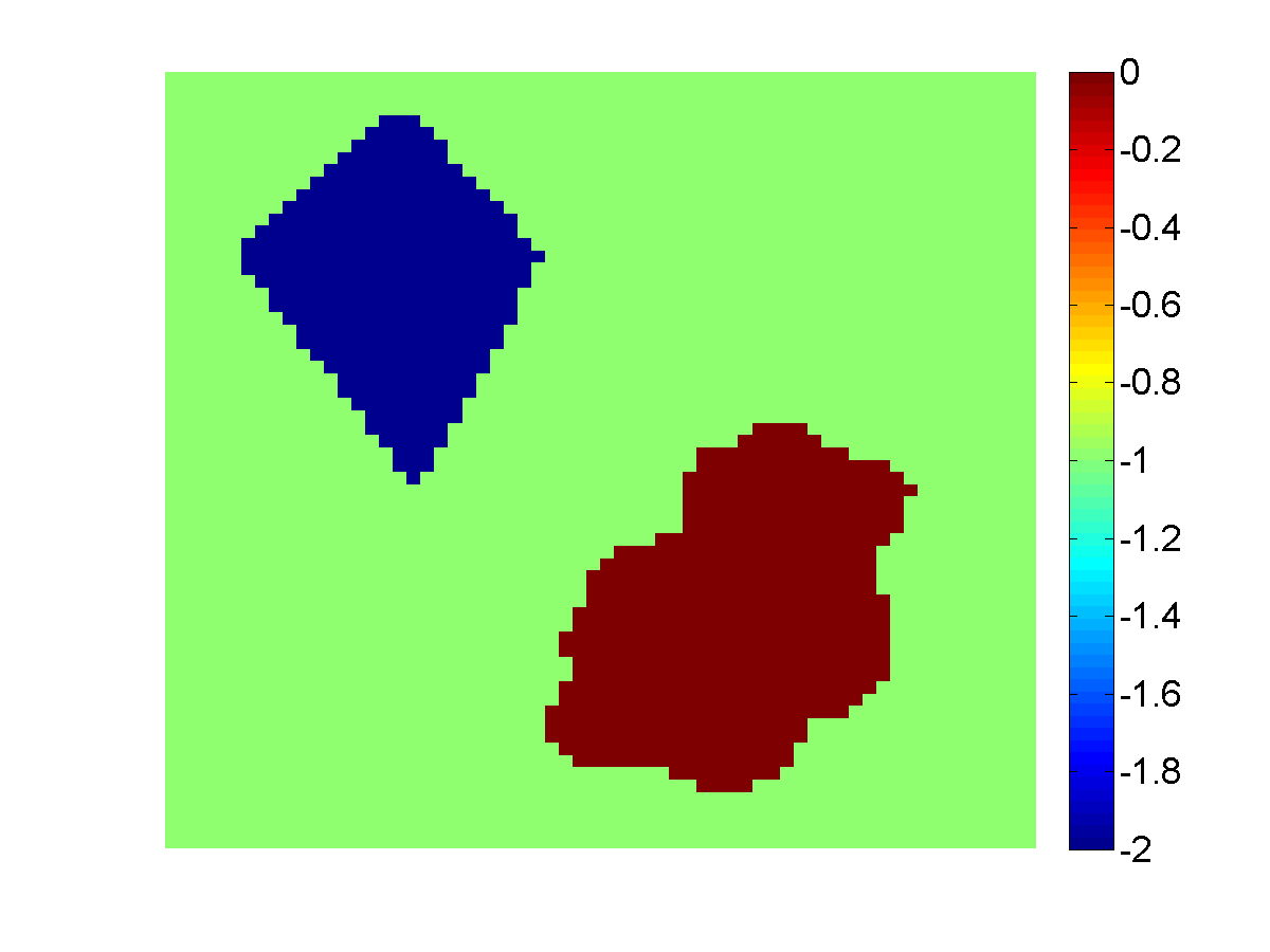
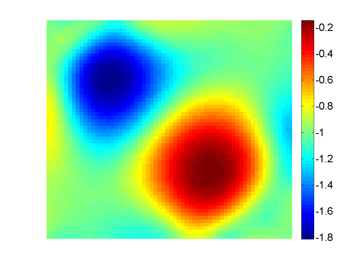
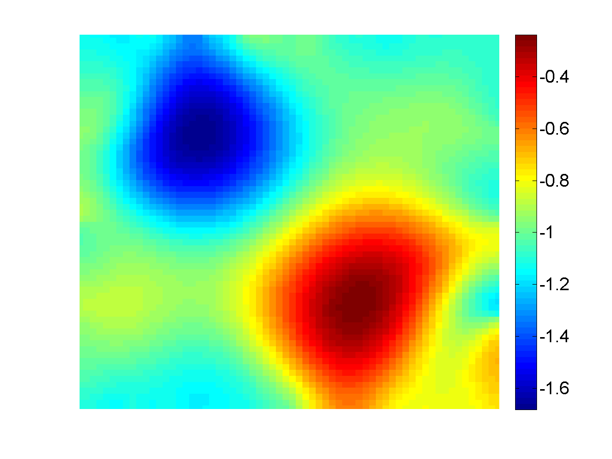
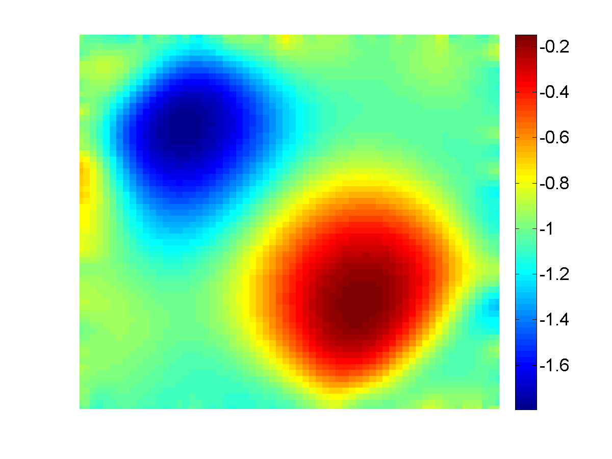
Figure 3: Plots of log-conductivity: (a) True model; (b) Vanilla recovery with $s=3,969$; (c) Vanilla recovery with $s=49$; (d) Monte Carlo recovery with $s=3,969$. The vanilla recovery using only $49$ measurement sets is clearly inferior, showing that a large number of measurement sets can be crucial for better reconstructions. The recovery using our algorithm, however, is comparable in quality to Vanilla with the same $s$. The quantifier values used in our algorithm were: $(\varepsilon_{c},\delta_{c})=(0.05,0.3)$, $(\varepsilon_{u},\delta_{u})=(0.1,0.3)$ and $(\varepsilon_{t},\delta_{t})=(0.1,0.1)$.

Figure 3 depicts an example of a piecewise constant “true model” ${\bf m}_{\rm true}$ consisting of two homogeneous but different bodies in a homogeneous background (a). This is used to synthesize noisy partial-boundary data sets that are then used in turn to approximately recover the model. The large dynamical range of the conductivities, together with the fact that the data is available only on less than half of the boundary, contribute to the difficulty in obtaining good quality reconstructions. The term “Vanilla” refers to using all $s$ available data sets for each task during the algorithm. This costs 527,877 PDE solves for $s=3,969$ (b) and 5,733 PDE solves for $s=49$ (c). However, the quality of reconstruction using the smaller number of data sets is clearly inferior. On the other hand, using our algorithm yields a recovery (d) that is comparable to Vanilla but at the cost of only 5,142 PDE solves. The latter cost is about 1% that of Vanilla and is comparable in order of magnitude to that of evaluating $\phi({\bf m})$ once!

4.1 TV and stochastic methods

This section, like Section 2.2.1, is not directly related to the main theme of this article, but it arises from the present discussion and has significant merit on its own. The two comments below are not strongly related to each other.

• The specific example considered above is used also in [47], except that the objective function there includes a total variation (TV) regularization. This represents usage of additional a priori information (namely, that the true model is discontinuous with otherwise flat regions), whereas here an implicit $\ell_{2}$-based regularization has been employed without such knowledge regarding the true solution. The results in Figures 4.3(b) and 4.4(vi) there correspond to our Figures 3(b) and 3(d), respectively, and as expected, they look sharper in [47]. On the other hand, a comparative glance at Figure 4.3(c) there vs the present Figure 3(c) reveals that the $\ell_{1}$-based technique can be inferior to the $\ell_{2}$-based one, even for recovering a piecewise constant solution! Essentially, even for this special solution form TV shines only with sufficiently good data, and here “sufficiently good” translates to “many data dets”. This intuitively obvious observation does not appear to be as well-known today as it used to be [18].

• If we run the code used to obtain the results displayed in this section and in [47] several times (having at first settled on whether or not to use TV regularization), different solutions ${\bf m}$ are obtained because of the different way that the noisy data sets are sampled. The variance of such solutions may provide information, or indication, on the extent to which, albeit having done our best to control the misfit function $\phi({\bf m})$, we can trust the quality of the reconstruction [49]. A large variance in ${\bf m}$ suggests a capricious dependence of the solution on the noisy data (that is given indirectly through $F({\bf m})$), and it would decrease our confidence in the computed results using a particular bias such as TV regularization. Having such information is an advantage of the stochastic algorithm over a similar determinstic one.

5 Conclusions and further notes

Mathematical software packages typically offer a default option for the error tolerances used in their implementation. Users often select this default option without much further thinking, at times almost automatically. This in itself suggests that practical occasions where the practitioner does not really have a good hold of a precise tolerance value are abundant. However, since it is often convenient to assume having such a value, and convenience may breed complacency, surprises may arise. We have considered in Section 2 four case studies which highlight various aspects of this uncertainty in a tolerance value for a stopping criterion.

Recognizing that there can often be a significant uncertainty regarding the actual tolerance value and the stopping criterion, we have subsequently considered the relaxation of the setting into a probabilistic one, and demonstrated its benefit in the context of the case study of Section 2.4. The environment defined by (20) or (25), although well-known in other research areas, is relatively new (but not entirely untried) in the numerical analysis community. It allows, among other benefits, specifying an amount of trust in a given tolerance using two parameters that can be tuned, as well as the development of bounds on the sample size of certain Monte Carlo methods, as described in Section 3. In Section 4 we have then applied this setting in the context of a particular inverse problem involving the solution of many PDEs, and we have obtained some uncertainty quantification for a rather efficient algorithm solving a large scale problem.

There are several aspects of our topic that remain untouched in this article. For instance, there is no discussion of the varying nature of the error quantity that is being measured (which strongly differs across the subsections of Section 2, from solution error through residual error through data misfit error for an ill-posed problem to stochastic quantities that relate even less closely to the solution error). Also, we have not mentioned that complex algorithms often involve sub-tasks such as solving a linear system of equations iteratively, or employing generalized cross validation (GCV) to obtain a tolerance value, or invoking some nonlinear optimization routine, which themselves require some stopping criterion: thus, several occurrences of tolerances in one solution algorithm are common. In the probabilistic sections, we have made the choice of concentrating on bounding the sample size $n$ and not, for example, on minimizing the variance as in [36].

What we have done here is to highlight an often ignored yet rather fundamental issue from different angles. Subsequently, we have pointed at and demonstrated a promising approach (or direction of thought) that is not currently common in the scientific computing community. Along the way we have also made in context several observations (Sections 2.1.1, 2.2.1, 2.3.1 and 4.1) from an array of fields of numerical computation, observations which we believe are not common knowledge.

References

- [1] D. Achlioptas. Database-friendly random projections. In ACM SIGMOD-SIGACT-SIGART Symposium on Principles of Database Systems, PODS ’01, volume 20, pages 274–281, 2001.
- [2] H. Akaike. On a successive transformation of probability distribution and its application to the analysis of the optimum gradient method. Ann. Inst. Stat. Math. Tokyo, 11:1–16, 1959.
- [3] S R Arridge. Optical tomography in medical imaging. Inverse Problems, 15(2):R41, 1999.
- [4] U. Ascher and C. Greif. First Course in Numerical Methods. Computational Science and Engineering. SIAM, 2011.
- [5] U. Ascher, R. Mattheij, and R. Russell. Numerical Solution of Boundary Value Problems for Ordinary Differential Equations. Classics. SIAM, 1995.
- [6] U. Ascher and L. Petzold. Computer Methods for Ordinary Differential and Differential-Algebraic Equations. SIAM, 1998.
- [7] U. Ascher and S. Reich. The midpoint scheme and variants for hamiltonian systems: advantages and pitfalls. SIAM J. Scient. Comput., 21:1045–1065, 1999.
- [8] H. Avron and S. Toledo. Randomized algorithms for estimating the trace of an implicit symmetric positive semi-definite matrix. JACM, 58(2), 2011. Article 8.
- [9] J. Barzilai and J. Borwein. Two point step size gradient methods. IMA J. Num. Anal., 8:141–148, 1988.
- [10] E. van den Berg and M. P. Friedlander. Probing the pareto frontier for basis pursuit solutions. SIAM J. Scient. Comput., 31(2):890–912, 2008.
- [11] D.A. Boas, D.H. Brooks, E.L. Miller, C. A. DiMarzio, M. Kilmer, R.J. Gaudette, and Q. Zhang. Imaging the body with diffuse optical tomography. Signal Processing Magazine, IEEE, 18(6):57–75, 2001.
- [12] L. Borcea, J. G. Berryman, and G. C. Papanicolaou. High-contrast impedance tomography. Inverse Problems, 12:835–858, 1996.
- [13] Y. Cao and L. Petzold. A posteriori error estimation and global error control for ordinary differential equations by the adjoint method. SIAM J. Scient. Comput., 26:359–374, 2004.
- [14] M. Cheney, D. Isaacson, and J. C. Newell. Electrical impedance tomography. SIAM Review, 41:85–101, 1999.
- [15] G. Dahlquist and A. Bjorck. Numerical Methods. Prentice-Hall, 1974.
- [16] Y. Dai and R. Fletcher. Projected Barzilai-Borwein methods for large-scale box-constrained quadratic programming. Numerische. Math., 100:21–47, 2005.
- [17] K. van den Doel and U. Ascher. The chaotic nature of faster gradient descent methods. J. Scient. Comput., 48, 2011. DOI: 10.1007/s10915-011-9521-3.
- [18] K. van den Doel, U. Ascher, and E. Haber. The lost honour of -based regularization. Radon Series in Computational and Applied Math, 2013. M. Cullen, M. Freitag, S. Kindermann and R. Scheinchl (Eds).
- [19] O. Dorn, E. L. Miller, and C. M. Rappaport. A shape reconstruction method for electromagnetic tomography using adjoint fields and level sets. Inverse Problems, 16, 2000. 1119-1156.
- [20] H. W. Engl, M. Hanke, and A. Neubauer. Regularization of Inverse Problems. Kluwer, Dordrecht, 1996.
- [21] A. Fichtner. Full Seismic Waveform Modeling and Inversion. Springer, 2011.
- [22] A. Friedlander, J. Martinez, B. Molina, and M. Raydan. Gradient method with retard and generalizations. SIAM J. Num. Anal., 36:275–289, 1999.
- [23] H. Gao, S. Osher, and H. Zhao. Quantitative photoacoustic tomography. In Mathematical Modeling in Biomedical Imaging II, pages 131–158. Springer, 2012.
- [24] A. Greenbaum. Iterative Methods for Solving Linear Systems. SIAM, 1997.
- [25] E. Haber, U. Ascher, and D. Oldenburg. Inversion of 3D electromagnetic data in frequency and time domain using an inexact all-at-once approach. Geophysics, 69:1216–1228, 2004.
- [26] E. Haber, M. Chung, and F. Herrmann. An effective method for parameter estimation with PDE constraints with multiple right-hand sides. SIAM J. Optimization, 22:739–757, 2012.
- [27] E. Haber, S. Heldmann, and U. Ascher. Adaptive finite volume method for distributed non-smooth parameter identification. Inverse Problems, 23:1659–1676, 2007.
- [28] E. Hairer, C. Lubich, and G. Wanner. Geometric Numerical Integration. Springer, 2002.
- [29] E. Hairer, S. Norsett, and G. Wanner. Solving Ordinary Differential Equations I. Springer, 1993.
- [30] E. Hairer and G. Wanner. Solving Ordinary Differential Equations II. Springer, 1996.
- [31] T. Hastie, R. Tibshirani, and J. Friedman. The Elements of Statistical Learning. Springer, 2001.
- [32] M. Heath. Scientific Computing, An Introductory Survey. McGraw-Hill, 2002. 2nd Ed.
- [33] F. Herrmann, Y. Erlangga, and T. Lin. Compressive simultaneous full-waveform simulation. Geophysics, 74:A35, 2009.
- [34] Desmond J. Higham. Global error versus tolerance for explicit runge-kutta methods. IMA J. Numer. Anal, 11:457–480, 1991.
- [35] J. Holodnak and I. Ipsen. Randomized approximation of the gram matrix: Exact computation and probabilistic bounds. SIAM J. Matrix Anal. Applic., 2014. to appear.
- [36] M.F. Hutchinson. A stochastic estimator of the trace of the influence matrix for laplacian smoothing splines. J. Comm. Stat. Simul., 19:433–450, 1990.
- [37] I. Ipsen and T. Wentworth. The effect of coherence on sampling from matrices with orthonormal columns, and preconditioned least squares problems. SIAM J. Matrix Anal. Applic., 2014. To appear.
- [38] J. Kaipo and E. Somersalo. Statistical and Computational Inverse Problems. Springer, 2005.
- [39] B. Leimkuhler and S. Reich. Simulating Hamiltonian Dynamics. Cambridge, 2004.
- [40] V. A. Morozov. Methods for Solving Incorrectly Posed Problems. Springer, 1984.
- [41] G. A. Newman and D. L. Alumbaugh. Frequency-domain modelling of airborne electromagnetic responses using staggered finite differences. Geophys. Prospecting, 43:1021–1042, 1995.
- [42] D. Oldenburg, E. Haber, and R. Shekhtman. 3D inverseion of multi-source time domain electromagnetic data. J. Geophysics, 2013. To appear.
- [43] A. Pidlisecky, E. Haber, and R. Knight. RESINVM3D: A MATLAB 3D Resistivity Inversion Package. Geophysics, 72(2):H1–H10, 2007.
- [44] M. Raydan. Convergence Properties of the Barzilai and Borwein Gradient Method. PhD thesis, Rice University, Houston, Texas, 1991.
- [45] J. Rohmberg, R. Neelamani, C. Krohn, J. Krebs, M. Deffenbaugh, and J. Anderson. Efficient seismic forward modeling and acquisition using simultaneous random sources and sparsity. Geophysics, 75(6):WB15–WB27, 2010.
- [46] F. Roosta-Khorasani and U. Ascher. Improved bounds on sample size for implicit matrix trace estimators. Foundations of Comp. Math., 2014. DOI: 10.1007/s10208-014-9220-1.
- [47] F. Roosta-Khorasani, G. Székely, and U. Ascher. Assessing stochastic algorithms for large scale nonlinear least squares problems using extremal probabilities of linear combinations of gamma random variables. SIAM/ASA J. Uncertainty Quantification, 2014. accepted, to appear.
- [48] F. Roosta-Khorasani, K. van den Doel, and U. Ascher. Stochastic algorithms for inverse problems involving PDEs and many measurements. SIAM J. Scientific Computing, 36(5):S3–S22, 2014.
- [49] A. Shapiro, D. Dentcheva, and D. Ruszczynski. Lectures on Stochastic Programming: Modeling and Theory. Piladelphia: SIAM, 2009.
- [50] N. C. Smith and K. Vozoff. Two dimensional DC resistivity inversion for dipole dipole data. IEEE Trans. on geoscience and remote sensing, GE 22:21–28, 1984.
- [51] U. Trottenberg, C. Oosterlee, and A. Schuller. Multigrid. Academic Press, 2001.
- [52] C. Vogel. Computational methods for inverse problem. SIAM, Philadelphia, 2002.
- [53] J. Young and D. Ridzal. An application of random projection to parameter estimation in partial differential equations. SIAM J. Scient. Comput., 34:A2344–A2365, 2012.
- [54] Z. Yuan and H. Jiang. Quantitative photoacoustic tomography: Recovery of optical absorption coefficient maps of heterogeneous media. Applied physics letters, 88(23):231101–231101, 2006.