Coherent control of non-Markovian photon resonator dynamics

Abstract

We study the unitary time evolution of photons interacting with a dielectric resonator using coherent control pulses. We show that non-Markovianity of transient photon dynamics in the resonator subsystem may be controlled to within a photon-resonator transit time. In general, appropriate use of coherent pulses and choice of spatial subregion may be used to create and control a wide range of non-Markovian transient dynamics in photon resonator systems.

I Introduction

The transient dynamics of photons interacting with a resonator is of both fundamental and practical interest. For example, microcavity resonators have been explored as a means to delay light in classical communication systems Yariv et al. (1999), and similar ideas have been developed for single photons Hach et al. (2010); Mirza et al. (2013); Shen and Fan (2009) with potential future use in quantum communication protocols. These and other studies exploit a basic property of a resonator subsystem, namely the ability to store photon energy density and release it at a later time. Since Markovian dynamics may be identified with information flow leaving the system Breuer et al. (2009), it seems natural to expect that storage of a photon or many photons in a resonator can result in non-Markovian behavior. More precisely, if we consider a finite region of a resonator, energy can both enter and leak out of the designated region depending on the interplay of system parameters and the location of the region itself. It seems natural to expect a high degree of non-Markovianity in such a situation. Furthermore, non-Markovianity may be viewed as a resource for information processing tasks Bylicka et al. (2013). One is therefore motivated to demonstrate control of photon transient dynamics and hence control of the associated non-Markovianity.

To investigate such non-Markovian effects we study the full time evolution of a Hamiltonian system and concentrate on the dynamics of a subregion obtained by tracing out exactly the remaining degrees of freedom. In a unitary system of finite spatial extent, excitations are reflected indefinitely back and forth from the boundaries, and consequently any subregion of such a system would always display non-Markovian behavior. The same holds true for a system with discrete energy levels because of the formation of bound states. To avoid these trivial cases, we seek therefore a system with a continuous energy spectrum such that the subsystem can exchange continuous energy with its environment as sketched in Fig. 1(a).

The physics we are interested in exploring may be captured by a single resonator with a refractive index profile as illustrated in Fig. 1(b). The symmetric one-dimensional Fabry-P/’erot resonator consists of three spatial regions, $A$, $B$, and $C$ in vacuum separated by two lossless dielectric mirrors, each of refractive index $n_{{\rm{r}}}$ and thickness $L_{{\rm{m}}}=\lambda_{0}/4n_{{\rm{r}}}$, where $\lambda_{0}$ is the resonant photon wavelength in vacuum. Spatial regions $A$ and $C$ connect to continuous input and output states at $x=x_{{\rm{A}}}$ and $x=x_{{\rm{C}}}$, respectively. The resonator cavity length is $L_{{\rm{B}}}$ and defines the spatial extent of region $B$. At the resonant photon wavelength, the complex mirror reflection amplitude is $re^{i\pi}=-r$, and the transmission amplitude is $te^{i\pi/2}=it$. Flux conservation in the lossless system requires $|r|^{2}+|t|^{2}=1$. Transmission through each mirror depends weakly on wavelength such that

$$|t|^{2}=\frac{1}{1+\left(\frac{k_{1}^{2}-k_{2}^{2}}{2k_{1}k_{2}}\right)^{2}\sin^{2}(k_{2}L_{{\rm{m}}})}\ ,$$ (1)

where the propagation constant in vacuum is $k_{1}=2\pi/\lambda$ and in the dielectric mirror it is $k_{2}=2\pi n_{{\rm{r}}}/\lambda$.

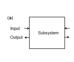
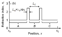
Figure 1: (a) Sketch of a subsystem with inputs and outputs to continuum states. (b) Symmetric Fabry-P/’erot resonator subsystem divided into spatial regions $A$, $B$, and $C$ separated by a quarter-wavelength lossless dielectric characterized by refractive index $n_{{\rm{r}}}$. The resonant wavelength is $\lambda_{0}$.

A single photon may be described by a wave function $\Psi(x,t)$ with the interpretation that $|\Psi(x,t)|^{2}$ is the photon energy density Bialynicki-Birula (1994); Sipe (1995); Smith and Raymer (2007). We choose to use a single-photon wave function description because, as will become apparent, it has the significant advantages in this initial study of both simplicity and ease of interpretation. The unitary dynamics of the photon wave function propagating in the $x$ direction in a lossless dielectric media may be modeled as a phase-coherent integral of linearly polarized basis states $\phi_{\omega}(x)$ with amplitudes $\alpha_{\omega}$ ,

$$\Psi(x,t)=\int\frac{d\omega}{2\pi}\alpha_{\omega}\phi_{\omega}(x)e^{-i\omega t}\ ,$$ (2)

where, as shown in the Appendix, $\phi_{\omega}(x)$ is a normalized solution of the one-dimensional Helmholtz equation,

$$\frac{d}{dx}\left(\frac{1}{\mu_{\mathrm{r}}(x)}\frac{d}{dx}\phi_{\omega}(x)\right)+\omega^{2}\epsilon_{\mathrm{r}}(x)\epsilon_{0}\mu_{0}\phi_{\omega}(x)=0\ .$$ (3)

The permeability of vacuum $\mu_{0}$ and permittivity of vacuum $\epsilon_{0}$ are related to the speed of light in vacuum via $c=1/\sqrt{\epsilon_{0}\mu_{0}}$. Assuming a lossless dielectric material, the spatial profile may be characterized by piecewise-constant values of relative permeability $\mu_{{\rm{r}}}$ and relative permittivity $\epsilon_{{\rm{r}}}$ in each region of the domain; the conditions imposed on $\phi_{\omega}(x)$ at the boundary between regions 1 and 2 at position $x_{0}$ are

$$\left.\phi_{\omega}(x)\right|_{x=x_{0}-\delta}=\left.\phi_{\omega}(x)\right|_{x=x_{0}+\delta}\ ,$$ (4)

and

$$\left.\frac{1}{\mu_{{\rm{r_{1}}}}}\frac{\mathrm{d}}{\mathrm{d}x}\phi_{\omega}(x)\right|_{x=x_{0}-\delta}=\left.\frac{1}{\mu_{{\rm{r_{2}}}}}\frac{\mathrm{d}}{\mathrm{d}x}\phi_{\omega}(x)\right|_{x=x_{0}+\delta}.$$ (5)

The refractive index is $n_{{\rm{r}}}=\sqrt{\mu_{{\rm{r}}}}\sqrt{\epsilon_{{\rm{r}}}}$. If we assume that the photon coherence time is longer than any other characteristic time scale, we may simply solve Eq. (3) to completely describe the evolution of the photon. In the thermodynamic limit there are a large number of photons in the system and Eq. (3) may also be used with the interpretation that the wave function corresponds to the classical electric field Bialynicki-Birula (1994); Sipe (1995); Smith and Raymer (2007). This means that our model simultaneously describes a single photon and a classical electromagnetic field.

An efficient and accurate way to solve Eq. (3) for the Fabry-P/’erot resonator subsystem coupled to continuous input and output states is to use the propagation matrix method Kane (1969); Levi (2014). All numerical simulations we present as part of our study use this method.

II Transient response

We consider the transient response of a rectangular single-photon pulse traveling left-to-right and incident on the Fabry-P/’erot resonator. We smoothen the rectangular pulse with center frequency $\omega_{0}$ by modulating a sinc function by a cosine in order to reduce the Gibbs phenomenon. In this way a rectangular pulse of duration $2T_{0}$ (length $2T_{0}c$) with rise and fall time $\tau_{{\rm{r}}}=2\pi/\Delta\omega_{{\rm{r}}}$ may be written as

$$\Psi(x,t) = \int\displaylimits_{\left|\omega-\omega_{0}\right|\leq\Delta\omega_{\mathrm{r}}}\frac{d\omega}{2\pi}\left(1+\cos\left(\frac{\pi(\omega-\omega_{0})}{\Delta\omega_{{\rm{r}}}}\right)\right)$$ (6)

$$\times\frac{\sin((\omega-\omega_{0})T_{0})}{(\omega-\omega_{0})T_{0}}\phi_{\omega}(x)e^{-i\omega t}\ .$$

To connect to existing photon technology we choose a cavity with resonant wavelength $\lambda_{0}=1500\ {\rm{nm}}$ and resonant frequency $\omega_{0}=2\pi/\tau_{0}$, where $\tau_{0}=5\ {\rm{fs}}$ corresponds to a resonant photon energy of $E_{0}=\hbar\omega_{0}=0.827\ {\rm{eV}}$. The refractive index of the mirrors is chosen to be $n_{{\rm{r}}}=2.5$, region $A$ has length $L_{{\rm{A}}}$, region $C$ has length $L_{{\rm{C}}}$ and, unless stated otherwise, the resonator cavity length is $L_{{\rm{B}}}=15\times\lambda_{0}$. The photon cavity round-trip time is $\tau_{{\rm{RT}}}=2L_{{\rm{B}}}/c=2\pi/\Delta\omega=30\times\tau_{0}=150\ {\rm{fs}}$, and the resonator quality factor is $Q=144$, where $\tau_{Q}=Q/\omega_{0}=114\ {\rm{fs}}$. Typically, one describes a transient response dominated by the ring-down time constant $\tau_{Q}=1/\Gamma$, where the photon energy density of a loaded resonator decays as $e^{-t/\tau_{Q}}$ and in which $\tau_{Q}$ is connected via a Fourier transform to a steady-state Lorentzian energy density spectrum Born et al. (1999); Saleh and Teich (2013) ,

$$S(\omega)=\frac{S_{0}}{(\omega-\omega_{0})^{2}+(\Gamma/2)^{2}}\ .$$ (7)

However, the actual transient dynamics of the system we wish to control is more complex than this description would suggest.

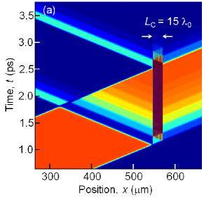
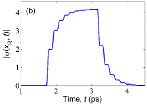
Figure 2: (color online) (a) Space-time photon energy density plot of a rectangular pulse incident on a Fabry-P/’erot resonator. The resonator is of length $L_{B}$ (indicated by two arrows). (b) $|\psi(x_{R},t)|$ (arbitrary scale) as a function of time detected at position $x_{R}$ far to the right of the resonator. The field decay constant $2\tau_{{\rm{Q}}}=229\ {\rm{fs}}$ is modulated by stepwise response at the resonant cavity round-trip time $\tau_{{\rm{RT}}}=30\tau_{0}=150\ {\rm{fs}}$. Photon pulse parameters are $\hbar\omega_{0}=0.827\ {\rm{eV}}$, $\hbar\Delta\omega_{{\rm{s}}}=0.207\ {\rm{eV}}$, and $T_{0}\omega_{0}=900$.

Figure 2(a) shows the calculated space-time photon energy density plot of a rectangular pulse initially moving left to right and incident on the Fabry-P/’erot resonator. The presence of the resonator imparts temporal structure onto reflected and transmitted photon energy density. The reflection at the leading edge and trailing edge of the incident pulse is due to frequency components associated with the pulse transient rise and fall times and the changing energy density in the resonator. Subsequent reflections decay temporally in a stepwise fashion in time steps of duration $\tau_{{\rm{RT}}}$. Figure 2(b) shows $|\Psi(x_{R},t)|$ calculated as a function of time detected at position $x_{R}$ far to the right of the resonator. Photon energy density both in the resonator and transmitted to position $x_{R}$ does not increase (or decay) as a simple exponential; rather, there is a stepwise buildup (or decay) at each resonant cavity photon round-trip time, $\tau_{{\rm{RT}}}$ O’Gorman et al. (1992). With increasing rectangular pulse duration, energy density asymptotically approaches the steady-state value, which, on resonance at frequency $\omega_{0}$, results in unity transmission and maximum energy density in the resonator. However, our interest is not the steady state; rather, we seek to coherently control the transient photon-resonator interaction using interference effects and in this way control non-Markovianity of the system. The shortest timescale on which we seek to exert control is the photon cavity transit time $\tau_{{\rm{RT}}}/2$.

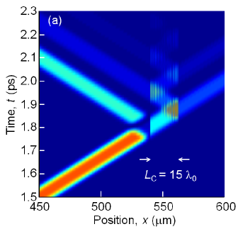
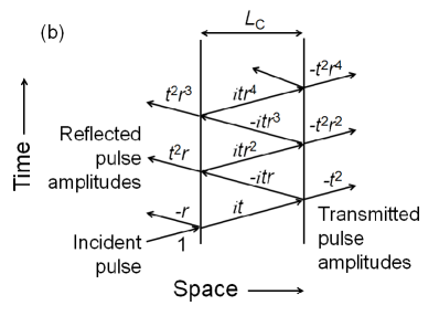
Figure 3: (a) Space-time photon energy density plot of a short rectangular pulse incident on the Fabry-P/’erot resonator showing ring-down. (b) Space-time resonant photon ray trace illustrating ring-down in the form of multiple transmitted and reflected amplitudes. Photon pulse parameters are $\hbar\omega_{0}=0.827\ {\rm{eV}}$, $\hbar\Delta\omega_{{\rm{s}}}=0.207\ {\rm{eV}}$, and $T_{0}\omega_{0}=60$.

Physical intuition and development of control concepts are best illustrated using a photon pulse whose duration is short compared to the cavity round-trip time, i.e., $2T_{0}<\tau_{{\rm{RT}}}$. Figure 3(a) shows the space-time photon energy density plot of a short rectangular pulse initially moving left-to-right and incident on the Fabry-P/’erot resonator. Initially, the photon energy density pulse entering the cavity shows no indication of wave character. It is only after reflection from the right mirror that self-interference effects are observed and photon resonances inside the cavity begin to build up. The energy stored in the resonator leaks out as forward and backscattered pulses. The shortest time between forward and backscattered pulses is the photon cavity transit time $\tau_{{\rm{RT}}}/2$.

Figure 3(b) illustrates the origin of the ring-down observed in the space-time diagram using space-time resonant photon ray tracing of reflected and transmitted amplitudes. The scattered amplitudes at each mirror form a geometric series.

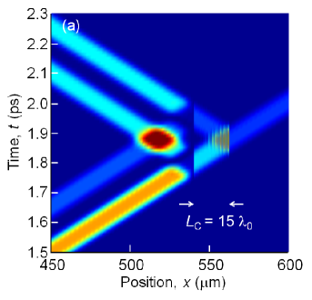
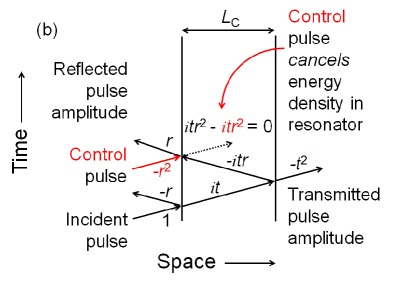
Figure 4: (a) Space-time photon energy density plot showing lead and control pulse. The control pulse eliminates ring-down by removing all photon energy density in the cavity after exactly one round-trip time, $\tau_{{\rm{RT}}}$. There is just one transmitted photon pulse. (b) Space-time resonant photon ray trace showing lead and control amplitudes configured to eliminate ring-down. Photon pulse parameters are $\hbar\omega_{0}=0.827\ {\rm{eV}}$, $\hbar\Delta\omega_{{\rm{s}}}=0.207\ {\rm{eV}}$, and $T_{0}\omega_{0}=60$.

III Coherent control of transient response

Coherent control of the transient response illustrated in Fig. 3 may be achieved using photon control pulses. Similar to Eq. (2), the control pulses consist of a coherent integral of basis functions whose amplitudes $\alpha_{\omega}^{{\rm{cont}}}$ and time delay $t_{\omega}^{{\rm{cont}}}$ are control parameters that can be optimized. In the following we avoid the use of formal optimization methods because the geometric series illustrated in Fig. 3(b) suggests a simpler intuitive approach.

First we consider a single control pulse that is just an attenuated, delayed, and phase-shifted version of the lead pulse. Figure 4(a) is a space-time photon energy density plot showing a lead pulse and control pulse initially moving left to right and incident on the Fabry-P/’erot resonator. In this example the control pulse is configured to eliminate ring-down after exactly one photon round-trip time in the cavity. This can be achieved with a control pulse of the same shape that is coherent with the lead pulse, with resonant amplitude $-r^{2}$ relative to the lead pulse, and delayed by a time $\tau_{{\rm{RT}}}$. Figure 4(b) is a space-time resonant photon ray trace showing lead and control amplitudes configured to eliminate ring-down.

To highlight the difference in the time domain between uncontrolled ring-down of the resonator and precise control, Fig. 5 shows the transmitted pulse train for the two situations illustrated in Figs. 3 and 4. Transmitted photon energy density as a function of time for the uncontrolled case [Fig. 5(a)] consists of a series of pulses whose peaks occur at equally spaced time intervals $\tau_{{\rm{RT}}}$ and whose peak value decreases exponentially as $e^{-t/\tau_{{\rm{Q}}}}$. For the controlled case [Fig. 5(b)] a coherent control pulse is used to ensure that there is just one transmitted photon energy density pulse.

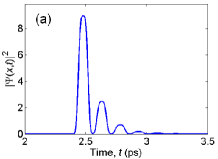
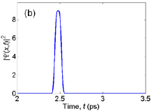
Figure 5: (a) Transmitted photon energy density as a function of time with no control (as in Fig. 3). (b) Same as (a) but with a control pulse to eliminate ring-down by removing all photon energy density in the cavity after exactly one round-trip time, $\tau_{{\rm{RT}}}$. There is just one transmitted photon pulse. Photon pulse parameters are $\hbar\omega_{0}=0.827\ {\rm{eV}}$, $\hbar\Delta\omega_{{\rm{s}}}=0.207\ {\rm{eV}}$, and $T_{0}\omega_{0}=60$. The photon energy density scale is arbitrary.

A coherent control pulse with amplitude $-r^{2N}$ injected at the $N$-th photon round trip may be used together with an integrating detector to evaluate a finite geometric sum. Figure 6(a) illustrates this for the case $N=3$. An integrating photon energy detector at the output measures this geometric sum as

$$\left|\sum_{n=0}^{N-1}ax^{n}\right|^{2}=\left|a\frac{1-x^{N}}{1-x}\right|^{2}\ ,$$ (8)

where, on resonance, $x=r^{2}$ and $a=t^{2}$. The sum in Eq. (8) is guaranteed to converge in the limit $N\to\infty$ because $|r|<1$.

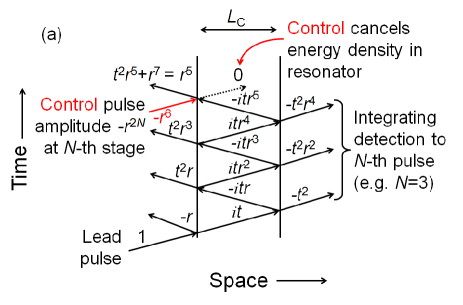
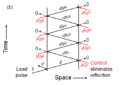
Figure 6: (color online) (a) Space-time resonant photon ray trace showing incident lead and control amplitudes configured to perform a finite geometric sum. (b) Space-time resonant photon ray trace showing incident lead photon and control amplitudes configured to create a finite divergent geometric series.

Figure 6(b) illustrates that the finite geometric series in Eq. (8) with $|x|>1$, may also be created by using multiple forward- and reverse-propagating control pulses. In this particular example coherent photon control pulses are used to confine photon energy density in the resonator. The photon energy density in the resonator increases according to Eq. (8) because $|r|<1$ and so $|x|=|e^{i\phi}/r|>1$, where $\phi$ is accumulated phase per cavity transit.

In general, transient photon dynamics in resonators with input and output ports may be used to evaluate arbitrary finite sums of the form

$$\left|\sum_{n=0}^{N-1}a_{n}x^{n}\right|^{2}\ ,$$ (9)

where complex $a_{n}$ and $x$ are determined by control pulses.

IV Coherent control of Markovianity

So far, we have demonstrated that coherent photon pulses can control transient photon dynamics in a resonant cavity. Here we wish to show that such techniques may be understood as controlling the degree of non-Markovianity exhibited by the system. To demonstrate control of non-Markovianity in the system it is necessary to adopt a suitable measure. The definition of a proper measure of non-Markovianity is currently a topic of debate and various, inequivalent, definitions have been proposed Breuer et al. (2009); Chruściński and Kossakowski (2010); Rivas et al. (2010); Chruściński et al. (2011); Bylicka et al. (2014). These definitions suffer from the drawback of being computationally demanding, and results have been reported only for extremely simple systems consisting of a single or a few qubits. Recently, a definition of non-Markovianity valid for Gaussian states (i.e., states satisfying the Wick theorem) has been proposed which has the advantage of being computationally tractable even for high-dimensional many-body systems Chancellor et al. (2014). In practice one asks if the dynamically evolving Gaussian state under consideration is consistent with quasifree Markovian dynamics in the sense of Refs. Prosen (2008); Prosen and Seligman (2010); Prosen (2010); Eisert and Prosen (2010). The answer is no if the Hilbert-Schmidt distance $D(t):=\left\|\Gamma_{1}(t)-\Gamma_{2}(t)\right\|_{HS}$ increases for some $t$ for initial states characterized by covariance matrices $\Gamma_{1,2}(0)$. More details on the precise definition of $D(t)$ may be found in Ref. Chancellor et al. (2014). In the following we are interested in establishing whether the exact evolution occurring in a spatial subregion $A$ can be considered Markovian according to the Hilbert-Schmidt distance. To check this we initialize the system with two different wave-packets $\Psi_{1}(x,0)$ and $\Psi_{2}(x,0)$ which are then evolved according to the exact equation of motion to $\Psi_{1}(x,t)$ and $\Psi_{2}(x,t)$. The Hilbert-Schmidt measure $D(t)$ takes the following form Chancellor et al. (2014)

$$D(t) =\frac{1}{\sqrt{2}}\sqrt{p_{1,1}^{2}+p_{2,2}^{2}-2\left|p_{1,2}\right|^{2}}$$ (10)

$$p_{i,j} =\int_{A}\Psi_{i}^{*}(x,t)\Psi_{j}(x,t)dx\,,$$ (11)

where in Eq. (11) the integral is performed over region $A$, one of the regions under examination. The system is considered Markovian if $D(t)$ decreases monotonically with time for any choice of initial state. Non-Markovianity is observed when $D(t)$ increases for a pair of initial states. Instead of considering all possible initial states, we are interested in quantifying the non-Markovian content of some physically motivated wave-packets $\Psi_{1}(x,t)$ and $\Psi_{2}(x,t)$. For simplicity we choose $\Psi_{2}(x,t)=\Psi_{1}(x,t+\tau_{{\rm{M}}})$ for a fixed delay $\tau_{{\rm{M}}}$.

As an example, consider a rectangular photon pulse propagating in free space and moving from left to right. It will freely enter, propagate, and exit the spatial region $A$. Figure 7(a) shows the resulting $D(t)$. Initially, both pulses are to the left of region $A$, so $D(t)=0$. As the first pulse $\Psi_{1}(x,t)$ enters the region, $D(t)$ increases, eventually reaching a value of $1/\sqrt{2}$. After time delay $\tau_{{\rm{M}}}$ the second pulse enters and increases $D(t)$ to its maximum value of unity, corresponding to both pulses simultaneously being in region $A$. There is a monotonic decrease in $D(t)$ as $\Psi_{1}(x,t)$ and $\Psi_{2}(x,t)$ leave and information leaks out of region $A$, indicating pure Markovian behavior.

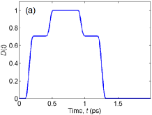
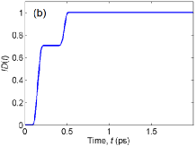
Figure 7: (a) Normalized measure $D(t)$ for rectangular photon pulse $\Psi_{1}(x,t)$ and $\Psi_{2}(x,t)=\Psi_{1}(x,t+\tau_{{\rm{M}}})$ freely propagating through spatial region $A$ of length $L_{{\rm{A}}}=160\times\lambda_{0}$. When both pulses are simultaneously in spatial region $A$, then $D(t)=1$. (b) $ID(t)$, the measure of non-Markovian dynamics for the pulse in (a). Photon pulse parameters are $\hbar\omega_{0}=0.827\ {\rm{eV}}$, $\hbar\Delta\omega_{{\rm{s}}}=0.207\ {\rm{eV}}$, $T_{0}\omega_{0}=60$, and $\tau_{{\rm{M}}}/\tau_{0}=60$.

A direct measure of non-Markovian dynamics is simply the positive contributions to $D(t)$. Defining $\sigma(t)=dD(t)/dt$, the total non-Markovian content after a time $t$ is

$$ID(t)=\int\displaylimits_{\sigma(\tau)>0\cap[0,t]}\,\sigma(\tau)d\tau\ .$$ (12)

The total non-Markovianity of the trajectories under consideration is $ID:=ID(\infty)$, where a larger value of $ID$ means more non-Markovian. Figure 7(b) shows the result of calculating $ID(t)$ for the non-interacting rectangular photon pulse considered in (a). As expected, after the two freely propagating pulses enter region $A$ there is no further increase in $ID(t)$. The purely Markovian dynamics of a system with no scattering results in a constant value for $ID(t)$.

Figure 8: (a) $D(t)$ for rectangular photon pulse $\Psi_{1}(x,t)$ and $\Psi_{2}(x,t)=\Psi_{1}(x,t+\tau_{{\rm{M}}})$ in spatial region $A$ [blue] to the left of the dielectric resonator and region $C$ [red] to the right of the resonator. $L_{{\rm{A}}}=160\times\lambda_{0}$ and $L_{{\rm{C}}}=120\times\lambda_{0}$. (c) $ID(t)$ for uncontrolled ring-down of $D(t)$ shown in (a). The calculated duration of non-Markovianity in region $A$ to the left of the dielectric resonator is limited by the pulse leaving the domain. (b) $D(t)$ and (d) $ID(t)$ illustrate the use of a single control pulse to reduce non-Markovianity in transient dynamics by removing all photon energy in the resonator after exactly one cavity round-trip time, $\tau_{{\rm{RT}}}$. Photon pulse parameters are $\hbar\omega_{0}=0.827\ {\rm{eV}}$, $\hbar\Delta\omega_{{\rm{s}}}=0.207\ {\rm{eV}}$, $T_{0}\omega_{0}=60$, and $\tau_{{\rm{M}}}/\tau_{0}=60$.

Photon dynamics are very different in the presence of a Fabry-P/’erot resonator because energy density can be scattered and stored. Figure 8 shows the result of calculating $D(t)$ and $ID(t)$ for a rectangular photon pulse initially incident from the left in spatial regions as defined in Figure 1(b). We ask whether the dynamics in finite-sized regions $A$ and $C$ can be considered Markovian and try to quantify its non-Markovianity content. Figures 8(a) and 8(c) show results for $D(t)$ and $ID(t)$ for a single initial rectangular pulse, while Figs.8(b) and 8(d) refer to the dynamics with a control pulse applied to remove all photon energy density inside the resonator after just one photon round-trip time $\tau_{{\rm{RT}}}$, as shown in Fig. 4(b).

The functions $D(t)$ and $ID(t)$ display complex temporal patterns, some features of which can readily be connected with the physics of the resonator. For example, consider the curve labelled $C$ in Fig. 8(c). Here we sent a control pulse whose effect is to eliminate completely the ring-down structure at the output (right) of the resonator. Consequently the single transmitted pulse has a behavior identical to that for the simple dynamics illustrated in Fig. 7.

However, a simple picture seems to emerge from Fig. 8, namely the total non-Markovian content of the dynamics restricted to region $C$ (right of the resonator) diminishes after application of the control pulse. On the other hand, the total non-Markovian content restricted to region $A$ (left of the resonator) increases in the presence of the control pulse. The sum of total non-Markovianity in regions $A$ and $C$ is greater for the uncontrolled case than for the controlled case.

Figure 9: $ID(t)$ for a resonator with cavity length $L_{{\rm{B}}}=120\times\lambda_{0}$, which defines region $B$, and a half space in the resonator cavity of length $L_{{\rm{B}}}/2$ adjacent to the left mirror, which defines region $B^{\prime}$. In the absence of a coherent control pulse, $ID(t)$ is purely Markovian for subspace $B$ and is non-Markovian for subspace $B^{\prime}$. Photon pulse parameters are $\hbar\omega_{0}=0.827\ {\rm{eV}}$, $\hbar\Delta\omega_{{\rm{s}}}=0.207\ {\rm{eV}}$, $T_{0}\omega_{0}=60$, and $\tau_{{\rm{M}}}/\tau_{0}=30$.

Non-Markovianity depends on subspace size and the location to which it is referred, so this naturally provides another approach to its control. For example, evaluating $D(t)$ in region $B$ inside the resonator involves spatial integrals over the entire cavity length, $L_{{\rm{B}}}$. However, if one evaluates $D(t)$ in a smaller portion of the cavity, then information flows in and out of that subspace as energy density builds up or decays in the resonator. Oscillatory values of $D(t)$ on a rising or falling background result, indicating non-Markovian contributions in a small subspace inside the resonator. These oscillations are averaged out when the subspace is increased to include the complete resonator cavity of length $L_{{\rm{B}}}$ (region $B$). This illustrates the fact that small subspaces can be tuned to exhibit enhanced non-Markovian effects.

To show how spatial placement of subspace determines Markovianity, consider a resonator with cavity length $L_{{\rm{B}}}=120\times\lambda_{0}$ that defines region $B$ and a half space in the resonator cavity of length $L_{{\rm{B}}}/2$ adjacent to the left mirror, which defines region $B^{\prime}$. As shown in Fig. 9, in the absence of coherent control, transient photon evolution dynamics is more non-Markovian for the half-cavity subspace $B^{\prime}$ than for the full-cavity subspace $B$. Placing the half-cavity subspace $B^{\prime}$ symmetrically about the center of the resonator does not remove non-Markovian dynamics. This is because resonator energy density stored outside $B^{\prime}$ is reflected by the mirrors back into $B^{\prime}$, causing the non-Markovian behavior.

V Conclusions

We have applied a Hilbert-Schmidt measure of non-Markovianity to a photon interacting with a symmetric lossless dielectric resonator. Non-Markovian transient photon dynamics in a resonator subsystem coupled to continuum states is shown to be controlled using coherent pulses. Transient photon dynamics can be controlled to within a photon resonator transit time. The underlying physical mechanisms used to control the dynamics at resonance are conveniently described using interference arising in finite geometric series with complex amplitudes. In general, coherent pulses, combined with a suitable choice of spatial subspace, may be used to both create and control a wide range of non-Markovian transient dynamics in photon-resonator systems. This initial study has revealed a richness in both the physics and control of single-photon transient dynamics interacting with a resonator, suggesting further study is warranted.

Appendix A The photon wave function

A.1 Introduction

To justify the use of the single photon wave function we present a simplified version of the arguments given in Refs. Bialynicki-Birula (1994); Sipe (1995); Smith and Raymer (2007); Abram (1987). This is done by first quantizing the electromagnetic field and restricting the discussion to wave propagation in one spatial dimension and lossless dielectrics. The corresponding quantized energy density operator in the dielectric is not diagonal when expressed in terms of the free-field operators. However, the energy density may be diagonalized through a unitary Bogolyubov transformation that relates the dielectric creation and annihilation operators to the free-field creation and annihilation operators. The abrupt perturbation at the air-dielectric interface may be viewed as projecting free-waves onto refracted waves using the “sudden approximation.” Continuity and smoothness are guaranteed via the field interface conditions.

A.2 The single-photon wave function in vacuum from the quantized electromagnetic field

The electromagnetic field in vacuum may be quantized in the Coulomb gauge to give:

$$\vec{A}(x^{\mu}) =\left(\frac{\hbar}{\epsilon_{0}}\right)^{1/2}\int\frac{d^{3}k}{(2\pi)^{3/2}}\frac{1}{\sqrt{2\omega}}$$

$$\times\sum_{r=1}^{2}\left(\vec{\epsilon}_{r}(\vec{k})a_{\vec{k},r}e^{-ik_{\mu}x^{\mu}}+\vec{\epsilon}_{r}(\vec{k})^{\ast}a_{\vec{k},r}^{\dagger}e^{ik_{\mu}x^{\mu}}\right)\ ,$$ (A.1a)

$$\vec{E}(x^{\mu}) =\left(\frac{\hbar}{\epsilon_{0}}\right)^{1/2}i\int\frac{d^{3}k}{(2\pi)^{3/2}}\sqrt{\frac{\omega}{2}}$$

$$\times\sum_{r=1}^{2}\left(\vec{\epsilon}_{r}(\vec{k})a_{\vec{k},r}e^{-ik_{\mu}x^{\mu}}-\vec{\epsilon}_{r}(\vec{k})^{\ast}a_{\vec{k},r}^{\dagger}e^{ik_{\mu}x^{\mu}}\right)\ ,$$ (A.1b)

$$\vec{B}(x^{\mu}) =\left(\frac{\hbar}{\epsilon_{0}}\right)^{1/2}i\int\frac{d^{3}k}{(2\pi)^{3/2}}\frac{1}{\sqrt{2\omega}}$$

$$\times\sum_{r=1}^{2}\left(\left(\vec{k}\times\vec{\epsilon}_{r}(\vec{k})\right)a_{\vec{k},r}e^{-ik_{\mu}x^{\mu}}\right.$$

$$\left.-\left(\vec{k}\times\vec{\epsilon}_{r}(\vec{k})^{\ast}\right)a_{\vec{k},r}^{\dagger}e^{ik_{\mu}x^{\mu}}\right),$$ (A.1c)

where $x^{\mu}=(ct,\vec{x})$, $k^{\mu}=(\omega/c,\vec{k})$, $\vec{\epsilon}_{r}$ is a polarization vector satisfying $\vec{k}\cdot\vec{\epsilon}_{r}(\vec{k})=0$, and $(a_{\vec{k},r},a_{\vec{k},r}^{\dagger})$ are annihilation and creation operators of a single plane wave excitation with momentum $\vec{k}$ and polarization $r$:

$$\left[a_{\vec{k},r},a_{\vec{k}^{\prime},s}^{\dagger}\right]=\delta_{rs}\delta^{(3)}(\vec{k}-\vec{k}^{\prime})\ .$$ (A.2)

The (normal ordered) Hamiltonian and momentum are, respectively, given by

$$:\!H\!: =\hbar\int d^{3}k\ \omega_{k}\sum_{r}a_{\vec{k},r}^{\dagger}a_{\vec{k},r}\ ,$$ (A.3)

$$:\!\vec{P}\!: =\hbar\int d^{3}k\ \vec{k}\sum_{r}a_{\vec{k},r}^{\dagger}a_{\vec{k},r}\ .$$ (A.4)

The vacuum $|0\rangle$ is defined by requiring $a_{k}|0\rangle=0$ for all $k$. The one-particle state

$$|\vec{k},r\rangle\equiv\sqrt{\frac{\omega_{k}}{c}}a_{\vec{k},r}^{\dagger}|0\rangle\ ,$$ (A.5)

is an eigenstate of the momentum operator with momentum $\vec{k}$ and polarization $r$. The reason for the $\sqrt{\omega_{k}}$ prefactor is that this makes the orthogonality condition given by

$$\langle\vec{k},r|\vec{k}^{\prime},r^{\prime}\rangle=\frac{\omega_{k}}{c}\delta^{(3)}(\vec{k}-\vec{k}^{\prime})\delta_{rr^{\prime}}\ ,$$ (A.6)

Lorentz invariant Peskin and Schroeder (1995). The one-particle completeness condition is then given by:

$$\openone_{\mathrm{1-particle}}=\sum_{r}\int d^{3}k\frac{c}{\omega_{k}}|\vec{k},r\rangle\langle\vec{k},r|\ .$$ (A.7)

For a momentum state with $\vec{k}=k\hat{e}_{z}$, we can choose $\vec{\epsilon}_{1}\equiv\vec{\epsilon}_{+}=-(\hat{e}_{x}+i\hat{e}_{y})/\sqrt{2}$, $\vec{\epsilon}_{2}\equiv\vec{\epsilon}_{-}=(\hat{e}_{x}-i\hat{e}_{y})/\sqrt{2}$, such that the momentum state satisfies

$$:\!H\!:\ |k\hat{e}_{z},\pm\rangle =\hbar ck|k\hat{e}_{z},\pm\rangle\ ,$$ (A.8)

$$:\!\vec{P}\!:\ |k\hat{e}_{z},\pm\rangle =\hbar k\hat{e}_{z}|k\hat{e}_{z},\pm\rangle\ ,$$ (A.9)

$$S_{z}|k\hat{e}_{z},\pm\rangle =\pm|k\hat{e}_{z},\pm\rangle\ ,$$ (A.10)

where $S_{z}=-i\hbar\left(\hat{e}_{x}\otimes\hat{e}_{y}-\hat{e}_{y}\otimes\hat{e}_{x}\right)$ is the $z$-component of the angular momentum operator. Therefore, let us consider a single particle state $|\psi\rangle$. We define the (vector) momentum space wave function of helicity $r$:

$$\vec{\psi}_{r}(\vec{k})=\langle\vec{k},r|\psi\rangle\ .$$ (A.11)

This is a vector due to the spin-1 nature of the photon and how the state must behave under the angular momentum operator. Furthermore, it satisfies

$$\vec{k}\cdot\vec{\psi}_{r}(\vec{k})=0\ .$$ (A.12)

The normalization of this momentum-space wave function is determined by the completeness condition:

$$1=\langle\psi|\psi\rangle=\sum_{r}\int d^{3}k\frac{c}{\omega_{k}}\vec{\psi}_{r}(\vec{k})^{\dagger}\vec{\psi}_{r}(\vec{k})\ .$$ (A.13)

This normalization of the momentum-space wave function matches that defined by Ref. Bialynicki-Birula (1994). We define the position-space wave function $\vec{\phi}(x)$ of the state to be simply the Fourier transform of $\vec{\psi}(k)$:

$$\vec{\phi}_{r}(\vec{x})=\int\frac{d^{3}k}{(2\pi)^{3/2}}e^{i\vec{k}\cdot\vec{x}}\vec{\psi}_{r}(\vec{k})\ .$$ (A.14)

This implies that

$$\langle\psi|:\!H\!:|\psi\rangle =\sum_{r}\int d^{3}x\ \vec{\phi}_{r}(\vec{x})^{\dagger}\vec{\phi}_{r}(\vec{x})$$

$$=\sum_{r}\int d^{3}k\ \vec{\psi}_{r}(\vec{k})^{\dagger}\vec{\psi}_{r}(\vec{k})\,,$$ (A.15)

Furthermore, Eq. (A.15) suggests that we interpret $\vec{\psi}_{r}(\vec{k})^{\dagger}\vec{\psi}_{r}(\vec{k})d^{3}k$ as the energy density in the shell $\vec{k}$ and $\vec{k}+d\vec{k}$ in momentum space rather than a probability density Smith and Raymer (2007). Finally, we note that

$$\langle\vec{k},\sigma|:\!H\!:|\psi\rangle =c\hbar|\vec{k}|\vec{\psi}_{\sigma}(\vec{k})$$

$$=c\hbar\sigma\left(\vec{s}\cdot\vec{k}\right)\vec{\psi}_{\sigma}(\vec{k})$$

$$=ic\hbar\sigma\vec{k}\times\vec{\psi}_{\sigma}(\vec{k})\,,$$ (A.16)

where $\vec{s}=(s_{x},s_{y},s_{z})$ are the three spin-1 matrices (generators of rotations for spin 1 particles; angular momentum is $\vec{S}=\hbar\vec{s}$), and we use the feature of spin-1 matrices that $\vec{a}\times\vec{b}=-i(\vec{a}\cdot\vec{s})\vec{b}$ Smith and Raymer (2007). Since the Hamiltonian is the generator of time translations, we have our Schr dinger equation:

$$i\hbar\partial_{t}\vec{\psi}_{\sigma}(\vec{k},t)=ic\hbar\sigma\vec{k}\times\vec{\psi}_{\sigma}(\vec{k},t)\ ,$$ (A.17)

or in position space,

$$i\hbar\partial_{t}\vec{\phi}_{\sigma}(\vec{x},t)=c\hbar\sigma\nabla\times\vec{\phi}_{\sigma}(\vec{x},t)\ .$$ (A.18)

Applying another $i\hbar\partial_{t}$, we recover the Helmholtz equation:

$$-\partial_{t}^{2}\vec{\phi}_{\sigma}(\vec{x},t)=c\nabla\times\left(c\nabla\times\vec{\phi}_{\sigma}(\vec{x},t)\right)=-c^{2}\nabla^{2}\vec{\phi}_{\sigma}(\vec{x},t)\ ,$$ (A.19)

where in the last equality we used Eq. (A.12).

A.3 Quantization in a linear lossless dielectric

One way to study the effect of the presence of the lossless linear medium is to consider the modified Hamiltonian density Abram (1987)

$$\mathcal{H}=\frac{1}{2}\left(\epsilon_{0}\vec{E}^{2}+\frac{1}{\mu_{0}}\vec{B}^{2}+\chi\vec{E}^{2}\right)\ .$$ (A.20)

(For other methods see Ref. Glauber and Lewenstein (1991).) Inserting the quantized fields in vacuum into this expression clearly shows that the Hamiltonian density operator is not diagonal in terms of the free-field creation and annihilation operators $(a_{\vec{k},\sigma}^{\dagger},a_{\vec{k},\sigma})$. Nevertheless, the Hamiltonian density can be diagonalized in terms of “refracted-wave” operators $(b_{\vec{k},\sigma}^{\dagger},b_{\vec{k},\sigma})$ via a Bogolyubov transformation Abram (1987). In this basis, the Hamiltonian density has the same eigenvalues as in vacuum, but the momentum operator is renormalized by a factor of the index of refraction, such that the results match the known results from classical optics.

At an abrupt vacuum-dielectric interface, where the permittivity changes from $\epsilon=\epsilon_{0}$ to $\epsilon=\sqrt{n_{{\rm{r}}}}\epsilon_{0}$, we can treat the change in the momentum operator (from the vacuum form to the renormalized form) in the “sudden approximation” Abram (1987). For example, a single excitation $a_{\vec{k},\sigma}^{\dagger,\sigma}|0\rangle$ gets projected to Abram (1987)

$$\left(\frac{2\sqrt{n_{{\rm{r}}}}}{n_{{\rm{r}}}+1}b_{\vec{k},\sigma}^{\dagger}+\frac{n_{{\rm{r}}}-1}{n_{{\rm{r}}}+1}a_{\vec{k},\sigma}^{\dagger}\right)|0\rangle\ ,$$ (A.21)

such that the probability of reflection and transmission agrees with the classical result for energy reflection and transmission. With these results in mind, we can generalize our equation for the single photon wave function to satisfy the Helmholtz equation in the presence of a lossless dielectric:

$$\nabla\times\left(\frac{1}{\mu(x)}\nabla\times\vec{\psi}_{\sigma}(\vec{x},t)\right)=-\epsilon(x)\partial_{t}^{2}\vec{\psi}_{\sigma}(\vec{x},t)\ .$$ (A.22)

For a linearly polarized, transverse field which propagates in the $x$ direction one has $\vec{\psi}_{\sigma}(\vec{x},t)=(0,\phi_{\sigma}(x,t),0)$, and one recovers Eq. (3) after a time Fourier transform.

References

- Yariv et al. (1999) A. Yariv, Y. Xu, R. K. Lee, and A. Scherer, Opt. Lett. 24, 711 (1999).
- Hach et al. (2010) E. E. Hach, A. W. Elshaari, and S. F. Preble, Phys. Rev. A 82, 063839 (2010).
- Mirza et al. (2013) I. M. Mirza, S. J. van Enk, and H. J. Kimble, J. Opt. Soc. Am. B 30, 2640 (2013).
- Shen and Fan (2009) J.-T. Shen and S. Fan, Phys. Rev. A 79, 023837 (2009).
- Breuer et al. (2009) H.-P. Breuer, E.-M. Laine, and J. Piilo, Phys. Rev. Lett. 103, 210401 (2009).
- Bylicka et al. (2013) B. Bylicka, D. Chruściński, and S. Maniscalco, ArXiv e-prints (2013), arXiv:1301.2585 .
- Bialynicki-Birula (1994) I. Bialynicki-Birula, Acta Phys. Pol. 86, 97 (1994).
- Sipe (1995) J. E. Sipe, Phys. Rev. A 52, 1875 (1995).
- Smith and Raymer (2007) B. J. Smith and M. G. Raymer, New J. Phys. 9, 414 (2007).
- Kane (1969) E. O. Kane, in Tunneling Phenomena in Solids, edited by E. Burstein and S. Lundqvist (Springer US, 1969) pp. 1–11.
- Levi (2014) A. Levi, Applied Quantum Mechanics (Cambridge University Press, 2014).
- Born et al. (1999) M. Born, E. Wolf, A. Bhatia, P. Clemmow, D. Gabor, A. Stokes, A. Taylor, P. Wayman, and W. Wilcock, Principles of Optics: Electromagnetic Theory of Propagation, Interference and Diffraction of Light (Cambridge University Press, 1999).
- Saleh and Teich (2013) B. Saleh and M. Teich, Fundamentals of Photonics, Wiley Series in Pure and Applied Optics (Wiley, 2013).
- O’Gorman et al. (1992) J. O’Gorman, A. F. J. Levi, D. Coblentz, T. Tanbun-Ek, and R. A. Logan, Appl. Phys. Letters 61, 889 (1992).
- Chruściński and Kossakowski (2010) D. Chruściński and A. Kossakowski, Phys. Rev. Lett. 104, 070406 (2010).
- Rivas et al. (2010) A. Rivas, S. F. Huelga, and M. B. Plenio, Phys. Rev. Lett. 105, 050403 (2010).
- Chruściński et al. (2011) D. Chruściński, A. Kossakowski, and A. Rivas, Phys. Rev. A 83, 052128 (2011).
- Bylicka et al. (2014) B. Bylicka, D. Chruściński, and S. Maniscalco, Sci. Rep. 4 (2014).
- Chancellor et al. (2014) N. Chancellor, C. Petri, L. Campos Venuti, A. F. J. Levi, and S. Haas, Phys. Rev. A 89, 052119 (2014).
- Prosen (2008) T. Prosen, New J. Phys. 10, 043026 (2008).
- Prosen and Seligman (2010) T. Prosen and T. H. Seligman, J. Phys. A 43, 392004 (2010).
- Prosen (2010) T. Prosen, J. Stat. Mech. 2010, P07020 (2010).
- Eisert and Prosen (2010) J. Eisert and T. Prosen, ArXiv e-prints (2010), arXiv:1012.5013 .
- Abram (1987) I. Abram, Phys. Rev. A 35, 4661 (1987).
- Peskin and Schroeder (1995) M. Peskin and D. Schroeder, An Introduction To Quantum Field Theory, Advanced book classics (Westview Press, 1995).
- Glauber and Lewenstein (1991) R. J. Glauber and M. Lewenstein, Phys. Rev. A 43, 467 (1991).