Quantum interference in HgTe structures

Abstract

We study quantum transport in HgTe/HgCdTe quantum wells under the condition that the chemical potential is located outside of the bandgap. We first analyze symmetry properties of the effective Bernevig-Hughes-Zhang Hamiltonian and the relevant symmetry-breaking perturbations. Based on this analysis, we overview possible patterns of symmetry breaking that govern the quantum interference (weak localization or weak antilocalization) correction to the conductivity in two dimensional HgTe/HgCdTe samples. Further, we perform a microscopic calculation of the quantum correction beyond the diffusion approximation. Finally, the interference correction and the low-field magnetoresistance in a quasi-one-dimensional geometry are analyzed.

I Introduction

Two-dimensional (2D) and three-dimensional (3D) materials and structures with strong spin-orbit interaction in the absence of magnetic field (i.e. with preserved time-reversal invariance) may exhibit a topological insulator (TI) phase Hasan10RMP ; Qi11 ; kane ; BernevigHughesZhang ; Koenig07 ; Fu07 ; hasan . In the 2D case, the TI behavior was experimentally discovered by the Würzburg group Koenig07 in HgTe/HgCdTe quantum wells (QWs) with band gap inversion due to strong spin-orbit interaction. The band inversion results in emergence of helical modes at the edge of the sample. These modes are topologically protected as long as the time-reversal symmetry is preserved.

Application of a bias voltage leads to the appearance of a quantized transverse spin current, which is the essence of the quantum spin-Hall effect (QSHE). An interplay between the charge and spin degrees of freedom characteristic to QSHE is promising for the spintronic applications. The existence of delocalized mode at the edge of an inverted 2D HgTe/HgCdTe QW was demonstrated in Refs. Koenig07, ; Roth09, . These experiments have shown that HgTe/HgCdTe structures realize a novel remarkable class of materials—$Z_{2}$ topological insulators—and thus opened a new exciting research direction. Another realization of a 2D $Z_{2}$ TI based on InAs/GaSb structures proposed in Ref. Liu08, was experimentally discovered in Ref. Du, .

When the chemical potential is shifted by applying a gate voltage away from the band gap, a HgTe/HgCdTe QW realizes a 2D metallic state which can be termed a 2D spin-orbit metal. The interference corrections to the conductivity and the low-field magnetoconductivity of such a system reflect the Dirac-fermion character of carriers ostrovsky10 ; Tkachov11 ; OGM12 ; Richter12 , similarly to interference phenomena in grapheneMcCann ; Nestoklon ; Ostrovsky06 ; aleiner-efetov and in surface layers of 3D TI ostrovsky10 ; Glazman ; Koenig13 . Recently, the magnetoresistivity of HgTe/HgCdTe structures was experimentally studied away from the insulating regime in Refs. kvon, ; minkov, ; bruene, , both for inverted and normal band ordering.

In this article we present a systematic theory of the interference-induced quantum corrections to the conductivity of HgTe-based structures in the metallic regime. We investigate the quantum interference in the whole spectrum, from the range of almost linear dispersion to the vicinity of the band bottom and address the crossover between the regimes. We begin by analyzing in Sec. II symmetry properties of the underlying Dirac-type Hamiltonian and physically important symmetry-breaking mechanisms. In Sec. III we overview a general symmetry-based approach OGM12 to the problem and employ it to evaluate the conductivity corrections within the diffusion approximation. Section IV complements the symmetry-based analysis by microscopic calculations. Specifically, we calculate the interference correction beyond the diffusion approximation, by using the kinetic equation for Cooperon modes which includes all the ballistic effects. A quasi one-dimensional geometry is analyzed in Sec. V. Section VI summarizes our results and discusses a connection to experimental works.

II Symmetry analysis of the low-energy Hamiltonian

The low-energy Hamiltonian for a symmetric HgTe/HgCdTe structure was introduced in Ref. BernevigHughesZhang, in the framework of the $\mathbf{k}\cdot\mathbf{p}$ method. The Bernevig-Hughes-Zhang (BHZ) Hamiltonian possesses a $4\times 4$ matrix structure in the Kramers-partner space and E1 – H1 space of electron- and hole-type levels Qi11 ; Liu08 ; Rothe10 ,

$$H_{\text{BHZ}}=\begin{pmatrix}h(\mathbf{k})&0\\ 0&h^{*}(-\mathbf{k})\end{pmatrix},$$ (1)

$$h(\mathbf{k})=\begin{pmatrix}\epsilon(\mathbf{k})+m(\mathbf{k})&A(k_{x}+ik_{y})\\ A(k_{x}-ik_{y})&\epsilon(\mathbf{k})-m(\mathbf{k})\end{pmatrix}.$$ (2)

Here the components of spinors are ordered as $E1+,H1+,E1-,H1-$. It is convenient to introduce Pauli matrices $\sigma_{0,x,y,z}$ for the E1—H1 space and $s_{0,x,y,z}$ for the Kramers-partner space (here $\sigma_{0}$ and $s_{0}$ are unity matrices), yielding

$$H_{\text{BHZ}}=\epsilon(\mathbf{k})\sigma_{0}s_{0}+m(\mathbf{k})\sigma_{z}s_{0}+Ak_{x}\sigma_{x}s_{z}-Ak_{y}\sigma_{y}s_{0}.$$ (3)

The effective mass $m(\mathbf{k})$ and energy $\epsilon(\mathbf{k})$ are given by

$$m(\mathbf{k})=M+B\mathbf{k}^{2},\qquad\epsilon(\mathbf{k})=C+D\mathbf{k}^{2},$$ (4)

The normal insulator phase corresponds to $M>0$ (which is realized in thin QWs, $d<6.2$ nm), whereas the TI phase is characterized by $M<0$ (realized in thick QW). Koenig07

The Hamiltonian $H_{\text{BHZ}}$ breaks up into two blocks that have the same spectrum

$$E^{\pm}_{\mathbf{k}}=\epsilon(\mathbf{k})\pm\sqrt{A^{2}k^{2}+m^{2}(\mathbf{k})}.$$ (5)

The eigenfunctions for each block are two-component spinors in E1-H1 space:

$$\psi_{\mathbf{k}}^{(\pm)}(\mathbf{r})=\chi_{\mathbf{k}}^{(\pm)}\,e^{i\mathbf{kr}}$$ (6)

where spinors $\chi_{\mathbf{k}}^{(\pm)}$ are different in different blocks

$$\chi_{\mathbf{k}}^{(\text{I},\pm)} =(1+\mu^{2}_{\pm})^{-1/2}\ \begin{pmatrix}1\\ \mu_{\pm}e^{-i\phi_{\mathbf{k}}}\end{pmatrix},$$ (7)

$$\chi_{\mathbf{k}}^{(\text{II},\pm)} =(1+\mu^{2}_{\pm})^{-1/2}\ \begin{pmatrix}1\\ -\mu_{\pm}e^{i\phi_{\mathbf{k}}}.\end{pmatrix}$$ (8)

Here $\phi_{\mathbf{\bf k}}$ is the polar angle of the momentum $\mathbf{k}$ and

$$\mu_{\pm}=\frac{\pm\left[A^{2}k^{2}+m^{2}(\mathbf{k})\right]^{1/2}-m(\mathbf{k})}{Ak}$$ (9)

corresponds to the upper and lower branches $E^{\pm}_{\mathbf{k}}$ of the spectrum.

Disorder potential $V(\mathbf{r})$ is conventionally introduced in the BHZ model by adding the scalar term Tkachov11

$$H_{\text{dis}}=V(\mathbf{r})\sigma_{0}s_{0}$$ (10)

to the $4\times 4$ Hamiltonian $H_{\text{BHZ}}$. This model describes smooth disorder that does not break the spatial reflection symmetry of the structure and thus does not mix the two Kramers blocks of the BHZ Hamiltonian.

We are now going to discuss symmetry properties of the Hamiltonian of a 2D HgTe/CdTe QW and symmetry-breaking mechanisms Rothe10 ; OGM12 . The Hamiltonian $H_{\text{BHZ}}+H_{\text{dis}}$ is characterized by the exact global time-reversal (TR) symmetry $H(\mathbf{k})=s_{y}H^{*}(-\mathbf{k})s_{y}$. Further, this Hamiltonian commutes with $s_{z}$, which we term the “spin symmetry”. Finally, an additional approximate symmetry operative within each Kramers block emerges for some regions of energy. Specifically, $h(\mathbf{k})$ in the inverted regime acquires the exact symplectic “block-wise” TR symmetry when $m(k_{F})=M+Bk_{F}^{2}=0$. Around this point, the symmetry is approximate. An approximate orthogonal block-wise TR symmetry emerges near the band bottom for $|M|\gg\{Ak_{F},Bk_{F}^{2}\}$ and for high energies $Bk_{F}^{2}\gg\{|M|,Ak_{F}\}$.

When employing the symmetry analysis to a realistic system, the symmetries of Hamiltonian (3) should be regarded as approximate. The term “approximate symmetry” here means that the corresponding symmetry breaking perturbations in the Hamiltonian are weak, such that they violate this “approximate symmetry” on scales that are much larger than the mean free path. On the technical level, the gaps of the corresponding soft modes (Cooperons) are small in this case. This, in turn, implies that there exists an intermediate regime, when the dephasing length (or the system size) is shorter than the corresponding symmetry-breaking length. In this regime, the diffusive logarithmic correction to the conductivity is insensitive to this symmetry-breaking mechanism and the system behaves as if this symmetry is exact. However, when the dephasing length becomes longer than the symmetry-breaking length, the relevant singular corrections are no longer determined by the dephasing but are cut off by the symmetry-breaking scale. This signifies a crossover to a different (approximate) symmetry class. Below we analyze the relevant symmetry-breaking perturbations in HgTe structures.

The $s_{z}$ spin symmetry is violated by perturbations that do not preserve the reflection ($z\to-z$) symmetry of the QW. Such perturbations yield nonzero block-off-diagonal elements in the full $4\times 4$ low-energy Hamiltonian. One of possible sources for the block mixing is the bulk inversion asymmetry (BIA) of the HgTe lattice. The corresponding term in the effective Hamiltonian reads Liu08

$$H_{\text{BIA}}=\begin{pmatrix}0&0&\delta_{e}k_{+}&-\Delta_{0}\\ 0&0&\Delta_{0}&\delta_{h}k_{-}\\ \delta_{e}k_{-}&\Delta_{0}&0&0\\ -\Delta_{0}&\delta_{h}k_{+}&0&0\end{pmatrix}.$$ (11)

The BIA perturbation (11) contains the momentum-independent term with $\Delta_{0}$ that connects the electronic and heavy-hole bands Winkler with opposite spin projections. The terms with $\delta_{e}$ and $\delta_{h}$ stem from the cubic Dresselhaus spin-orbit interaction within $\Gamma_{6}$ and $\Gamma_{8}$, respectively. Further, the $s_{z}$ symmetry is broken by the Rashba spin-orbit interaction due to the structural inversion asymmetry (SIA):Liu08 ; Rothe10

$$H_{R}=\begin{pmatrix}0&0&ir_{e}k_{-}&0\\ 0&0&0&0\\ -ir_{e}k_{+}&0&0&0\\ 0&0&0&0\end{pmatrix},$$ (12)

Here only the linear-in-momentum E1 SIA term is retained, as the SIA terms for heavy holes contain higher powers of $k$. Finally, short-range impurities and defects, as well as HgTe/HgCdTe interface roughness may also violate the $z\to-z$ symmetry of the QW, giving rise to a random local block-off-diagonal perturbations.

III Symmetry analysis of quantum conductivity corrections

Here we overview the approach developed in Ref. OGM12, for the analysis of quantum-interference corrections to the conductivity of an infinite 2D HgTe QW. Within the diffusion approximation, conductivity corrections that are logarithmic in temperature $T$ are associated with certain TR symmetries. The TR symmetry transformations can be represented as anti-unitary operators that act on a given operator $\mathcal{O}$ according to

$$T:\quad\mathcal{O}\mapsto U^{-1}\mathcal{O}^{T}U.$$

Here $U$ is some unitary operator (note that the momentum operator changes sign under transposition).

When the Hamiltonian of the system is given by a $4\times 4$ matrix, possible TR symmetry transformations can be cast in the form involving the tensor products of Pauli matrices:

$$T_{ij}:\quad\mathcal{O}\mapsto\sigma_{i}s_{j}\mathcal{O}^{T}s_{j}\sigma_{i},\quad i,j=0,x,y,z.$$ (13)

Each of these TR symmetries corresponds to a Cooperon mode contributing to the singular one-loop conductivity correction:

$$\delta\sigma_{ij}=-c_{ij}\frac{e^{2}}{2\pi h}\ln\left(\frac{\tau_{\phi}}{\tau}\right),\qquad c_{ij}=-1,\ 0,\ 1.$$ (14)

Here $\tau_{\phi}$ is the phase-breaking time due to inelastic scattering and $\tau$ is the transport time. The factors $c_{ij}$ in Eq. (14) are zero when the TR symmetry $T_{ij}$ is broken by the Hamiltonian; otherwise, $c_{ij}=T_{ij}^{2}=\pm 1$ for the orthogonal and symplectic type of the TR symmetry, respectively. The above perturbative loop expansion is justified by the large parameter $E_{F}\tau\gg 1$, where $E_{F}$ is the Fermi energy counted from the bottom of the band.

An analogous symmetry analysis of the interference effects was performed for a related problem of massless Dirac fermions in graphene in Ref. Ostrovsky06, . In Ref. OGM12, this approach was generalized to the case of massive Dirac fermions in a HgTe QW. By choosing the basis H1+,E1+,E1-,H1-, the linear-in-$k$ term in the BHZ Hamiltonian acquires the same structure as in Ref. Ostrovsky06, :

$$H_{BHZ}=\epsilon(\mathbf{k})\sigma_{0}s_{0}+[-m(\mathbf{k})\sigma_{z}+A\mathbf{k}{\bm{\sigma}}]s_{z}.$$ (15)

When the chemical potential is located in the range of approximately linear spectrum, $E_{\pm}\simeq\pm A|k|$, the Dirac mass $H_{M}=-m(\mathbf{k})\sigma_{z}s_{z}$ and the $s_{z}$-symmetry breaking terms

$$H_{\text{BIA}} =\Delta_{0}\sigma_{z}s_{x}+\delta_{+}(k_{x}\sigma_{x}+k_{y}\sigma_{y})s_{x}$$

$$\qquad+\delta_{-}(k_{x}\sigma_{y}-k_{y}\sigma_{x})s_{y},$$ (16)

$$H_{R} =(r_{e}/2)[(k_{x}\sigma_{y}+k_{y}\sigma_{x})s_{x}-(k_{x}\sigma_{x}-k_{y}\sigma_{y})s_{y}],$$ (17)

[where $\delta_{\pm}=(\delta_{h}\pm\delta_{e})/2$] can be treated as weak perturbations to the massless (graphene-like) Dirac Hamiltonian:

$$H_{A}=A(k_{x}\sigma_{x}+k_{y}\sigma_{y})s_{z}.$$ (18)

The latter possesses four TR symmetries:

$$T_{xx}: \quad\mathcal{O}\mapsto\sigma_{x}s_{x}\mathcal{O}^{T}\sigma_{x}s_{x},\qquad T_{xx}^{2}=1,$$ (19)

$$T_{y0}: \quad\mathcal{O}\mapsto\sigma_{y}s_{0}\mathcal{O}^{T}\sigma_{y}s_{0},\qquad T_{y0}^{2}=-1,$$ (20)

$$T_{yz}: \quad\mathcal{O}\mapsto\sigma_{y}s_{z}\mathcal{O}^{T}\sigma_{y}s_{z},\qquad T_{yz}^{2}=-1,$$ (21)

$$T_{xy}: \quad\mathcal{O}\mapsto\sigma_{x}s_{y}\mathcal{O}^{T}\sigma_{x}s_{y},\qquad T_{xy}^{2}=-1.$$ (22)

These symmetries give rise to a positive weak antilocalization (WAL) conductivity correction

$$\delta\sigma=-(1-3)\frac{e^{2}}{2\pi h}\ln\left(\frac{\tau_{\phi}}{\tau}\right)=2\times\frac{e^{2}}{2\pi h}\ln\left(\frac{\tau_{\phi}}{\tau}\right),$$ (23)

corresponding to two independent copies of a symplectic-class system (2Sp).

The mass term $H_{M}=-m(\mathbf{k})\sigma_{z}s_{z}$ violates $T_{y0}$ and $T_{yz}$ symmetries footnote_mass on the scale determined by the symmetry breaking rate Tkachov11 ; OGM12 $1/\tau_{m}\sim[m(k_{F})/E_{F}]^{2}/\tau$ (see Sec. IV below for the microscopic derivation). The two out of four soft modes acquire the gap $\tau/\tau_{m}$, yielding

$$\delta\sigma=-2\times\frac{e^{2}}{2\pi h}\ln\left(\frac{\tau}{\tau_{\phi}}+\frac{\tau}{\tau_{m}}\right).$$ (24)

At lowest temperatures, when $\tau_{\phi}\gg\tau_{m}$, we find a nonsingular-in-$T$ result:

$$\delta\sigma\simeq 2\times\frac{e^{2}}{2\pi h}\ln\left(\frac{\tau_{m}}{\tau}\right).$$ (25)

For higher temperatures, when $\tau_{\phi}\ll\tau_{m}$, these two copies of a unitary-class system (2U) become two copies of the (approximately) symplectic class, with the correction given by Eq. (23).

In the presence of inversion-asymmetry terms $H_{\text{BIA}}$ and $H_{R}$, the only remaining TR symmetry is $T_{xy}$. The symmetry analysis yields the following expression for the conductivity correction in this (generic) case OGM12 :

$$\delta\sigma=\frac{e^{2}}{2\pi h}\Bigg{[}\ln\left(\frac{\tau}{\tau_{\phi}}+\frac{\tau}{\tau_{\Delta}}+\frac{\tau}{\tau_{\text{SO}}}\right)\\ -\ln\left(\frac{\tau}{\tau_{\phi}}+\frac{\tau}{\tau_{m}}+\frac{\tau}{\tau_{\Delta}}+\frac{\tau}{\tau_{\text{SO}}}\right)\\ -\ln\left(\frac{\tau}{\tau_{\phi}}+\frac{\tau}{\tau_{m}}+\frac{\tau}{\tau_{\text{SO}}}\right)-\ln\frac{\tau}{\tau_{\phi}}\Bigg{]}.$$ (26)

Here $1/\tau_{\Delta}$ is the symmetry-breaking rate due to the $k$-independent term $\Delta_{0}\sigma_{z}s_{x}$ in $H_{\text{BIA}}$ while $1/\tau_{SO}$ describes the $s_{z}$-symmetry breaking governed by linear-in-$k$ terms in $H_{\text{BIA}}$ and $H_{R}$.

Thus the behavior of the conductivity at the lowest $T$ is governed by the single soft mode which reflects the physical symplectic TR symmetry $T_{xy}$. This mode yields a WAL correction characteristic for a single copy of the symplectic class system (1Sp). At higher temperatures, depending on the hierarchy of symmetry-breaking rates, the folllowing patterns of symmetry breaking can be realized: OGM12

• $\tau\ll\tau_{m}\ll\text{min}[\tau_{\Delta},\tau_{SO}]$: 2Sp $\to$ 2U $\to$ 1Sp;

• $\tau\ll\text{min}[\tau_{\Delta},\tau_{SO}]\ll\tau_{m}$: 2Sp $\to$ 1Sp.

• $\tau_{\text{SO}}\lesssim\tau$ or $\text{max}[\tau_{m},\tau_{\Delta}]\lesssim\tau$: 1Sp.

We now turn to the case when the chemical potential is located in the bottom of the spectrum, $E_{F}\ll|m|$. In this limit, the spectrum is approximately parabolic:

$$E_{+}(\mathbf{k}) \simeq |M|+Bk^{2}+\epsilon(\mathbf{k})+A^{2}k^{2}/|M|.$$ (27)

The direction of the pseudospin within each block is almost frozen by the effective “Zeeman term” $M$. The linear-in-$k$ terms of the BHZ Hamiltonian can then be treated as a weak spin-orbit-like perturbation to the massive diagonal Hamiltonian

$$H_{M}=-m(\mathbf{k})\sigma_{z}s_{z}.$$ (28)

Neglecting the block mixing, the conductivity is given by a sum of two weak localization (WL) corrections characteristic for an orthogonal symmetry class:

$$\delta\sigma=2\times\frac{e^{2}}{2\pi h}\ln\left(\frac{\tau}{\tau_{A}}+\frac{\tau}{\tau_{\phi}}\right).$$ (29)

Here $1/\tau_{A}\sim[Ak_{F}/m(k_{F})]^{4}/\tau$ is the symmetry-breaking rate due to “relativistic” correction $H_{A}$. The microscopic derivation of $1/\tau_{A}$ is performed in Sec. IV below.

The TR symmetries of the Hamiltonian $H_{M}$ can be combined into four pairs:

$$T_{00}\sim T_{zz},\quad T_{0z}\sim T_{z0},\quad T_{xx}\sim T_{yy},\quad T_{xy}\sim T_{yx}.$$

Symmetry breaking perturbations can affect the symmetries from each pair in different ways. When both TR symmetries from the pair are respected by the perturbation, the full Hamiltonian decouples into two blocks corresponding to the eigenvalues of $\sigma_{z}s_{z}$. Such a pair contributes to the conductivity as if there is a single TR symmetry. If only one of the two TR symmetries is broken within the pair, the remaining symmetry yields a conventional singular contribution. Finally, when both symmetries within the pair are broken, such pair does not contribute.

Thus, when both symmetries are not simultaneously violated, each pair contributes as a single soft mode. Note that in this case the corresponding Cooperon mass is determined by the sum of symmetry-breaking times rather than by the sum of rates. Following this rule, the inclusion of $H_{A}$, $H_{\text{BIA}}$, and $H_{R}$ gives rise to the following interference correction: OGM12

$$\delta\sigma=\frac{e^{2}}{2\pi h}\Bigg{[}2\ln\left(\frac{\tau}{\tau_{\phi}}+\frac{\tau}{\tau_{A}}+\frac{\tau}{\tau_{SO}}\right)\\ +\ln\left(\frac{\tau}{\tau_{\phi}}+\frac{\tau}{\tau_{SO}}+\frac{\tau}{\tau_{A}+\tau_{\Delta}}\right)-\ln\frac{\tau}{\tau_{\phi}}\Bigg{]}.$$ (30)

The only true massless mode in Eq. (30) stems again from the physical symplectic TR symmetry $T_{xy}$. This means that the generic block-mixing terms drive the two copies of the (approximately) orthogonal class to a single copy of a symplectic-class system. The hierarchy of the symmetry-breaking rates $\tau_{A}^{-1}$, $\tau_{\Delta}^{-1}$, and $\tau_{SO}^{-1}$, generates the following three patterns of crossovers:OGM12

• $\tau\ll\tau_{A}\ll\text{min}[\tau_{\Delta},\tau_{SO}]$: 2O $\to$ 2U $\to$ 1Sp.

• $\text{min}[\tau_{\Delta},\tau_{SO}]\ll\tau_{A}$ and $\tau\ll\text{min}[\tau_{A},\tau_{SO}]$:
  aa 2O $\to$ 1Sp.

• $\tau_{SO}\lesssim\tau$: 1Sp.

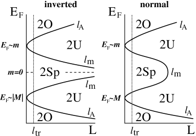
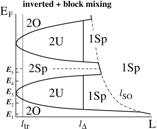
Figure 1: “Phase diagrams” showing the symmetry patterns for the quantum correction to the conductivity in a 2D HgTe QW when the chemical potential is located away from the bandgap, $E_{F}>0$. The length $L$ is the smallest of the system size or the dephasing length $L_{\phi}$. The transport scattering length $l_{\text{tr}}$ (shown by a vertical dotted line) and the BIA-splitting length $l_{\Delta}=(D\tau_{\Delta})^{1/2}$ ($D$ is the diffusion constant) are assumed to be independent of energy. The “phase boundaries” (solid lines) of the 2U-regions are defined by $l_{m}=(D\tau_{m})^{1/2}$ for 2Sp $\to$ 2U crossover, and by $l_{A}=(D\tau_{A})^{1/2}$ for 2O $\to$ 2U crossover. Left panel: Inverted band structure (thick quantum well) with no block mixing. Dashed line shows energy for which $m(k_{F})=-|M|+Bk_{F}^{2}=0.$ Middle panel: Normal band structure (thin quantum well) with no block mixing. Right panel: Inverted band structure with block mixing characterized by $l_{\Delta}=(D\tau_{\Delta})^{1/2}$ and $l_{\text{SO}}=(D\tau_{SO})^{1/2}$ (dash-dotted), with $\tau<\tau_{\Delta}<\tau_{SO}$. The energies $E_{F}=E_{1}\ldots E_{5}$ (from bottom to top) mark different horizontal cross-sections of the “phase-diagram” corresponding to the patterns 2O $\to$ 1Sp, 2O $\to$ 2U $\to$ 1Sp, 2U $\to$ 1Sp, 2Sp $\to$ 2U $\to$ 1Sp, and 2Sp $\to$ 1Sp, respectively, that appear with increasing $L$. The perturbative one-loop results discussed in Sec. III require the condition $E_{F}>1/\tau$, which introduces an additional horizontal line near the band bottom in all the panels. Further, we assume that the localization length in the 2U and 2O regions is smaller than the scale $L$.

To summarize this section, we have analyzed the quantum conductivity correction in the diffusion approximation using the symmetry-based approach. We have identified various possible types of behavior that include 2O, 2U, 2Sp, and 1Sp regimes. The $T$-dependence of the conductivity correction is given by $\delta\sigma=\alpha(e^{2}/\pi h)\ln\tau_{\phi}(T)$, where $\alpha=-1,0,1$, and $1/2$, respectively. The “phase diagram” describing these regimes is shown in Fig. 1.

In general, crossovers between the regimes are governed by four symmetry breaking rates: $1/\tau_{SO},$ $1/\tau_{\Delta},$ $1/\tau_{m},$ and $1/\tau_{A}$. The first two describe a weak block mixing in the BHZ Hamiltonian. They are present for arbitrary position of the Fermi energy and are assumed to be smaller than $1/\tau$. Near the band bottom (and for very high energies, where the spectrum is no longer linear) the “intra-block” rates satisfy: $\tau/\tau_{m}\sim 1$, while $\tau/\tau_{A}\ll 1$. In the region of linear spectrum the relations are opposite: $\tau/\tau_{m}\ll 1$, while $\tau/\tau_{A}\sim 1$.

Assuming for simplicity the absence of the BIA splitting of the spectrum, $1/\tau_{\Delta}=0,$ the general expression for the conductivity correction can be written as:

$$\delta\sigma = \frac{e^{2}}{4\pi^{2}\hbar}\times\left[2\ln\left(\frac{\tau}{\tau_{\phi}}+\frac{\tau}{\tau_{A}}+\frac{\tau}{\tau_{SO}}\right)\right.$$ (31)

$$- \left.2\ln\left(\frac{\tau}{\tau_{\phi}}+\frac{\tau}{\tau_{m}}+\frac{\tau}{\tau_{SO}}\right)\right.$$

$$+ \left.\ln\left(\frac{\tau}{\tau_{\phi}}+\frac{\tau}{\tau_{SO}}\right)-\ln\left(\frac{\tau}{\tau_{\phi}}\right)\right].$$

The first term here describes two copies (decoupled blocks) of WL near the band bottom, the second term describes two copies (decoupled blocks) of WAL in the range of linear dispersion, and the last two terms reflect a block mixing due to the spin-orbit interaction/scattering (they are present at any energy).

IV Microscopic calculation of the interference correction

In this section, we present a microscopic calculation of the interference correction to the conductivity for white-noise disorder beyond the diffusive approximation. We first consider the model with decoupled blocks and later analyze the effect of block mixing.

The WAL correction for decoupled blocks was studied in Ref. Tkachov11, within the diffusive approximation for the case when the chemical potential is located in the almost linear range of the spectrum. It was shown there that the finite bandgap (leading to a weak nonlinearity of dispersion) suppresses the quantum interference on large scales. Here we calculate the interference-induced conductivity correction in the whole range of concentrations and without relying on the diffusion approximation. This allows us to describe analytically the crossover from the WL behavior near the band bottom to the WAL in the range of almost linear spectrum. We compare our results to those of Ref. Tkachov11, in the end of Sec. IV.2.

For simplicity, we will consider the case $B=C=D=0$. Then the two blocks of the BHZ Hamiltonian read:

$$H_{\text{I}} = \left[\begin{array}[]{cc}M&A(k_{x}+ik_{y})\\ A(k_{x}-ik_{y})&-M\\ \end{array}\right],$$ (34)

$$H_{\text{II}} = \left[\begin{array}[]{cc}M&-A(k_{x}-ik_{y})\\ -A(k_{x}+ik_{y})&-M\\ \end{array}\right].$$ (37)

A generalization onto the case of $k$-dependent mass $m(\textbf{k})$ is straightforward. For definiteness, we will consider the block $H_{\text{II}}$.

The bare Green’s function of the system is a $2\times 2$ matrix in E1-H1 space which can be represented as a sum of the contributions of upper and lower branches:

$$\hat{G}(E,\mathbf{p})=\frac{\hat{P}_{+}(\mathbf{k})}{E-E^{+}_{\mathbf{k}}}+\frac{\hat{P}_{-}(\mathbf{k})}{E-E^{-}_{\mathbf{k}}},$$ (38)

where the projectors $\hat{P}_{\pm}$ are given by

$$\hat{P}_{\pm}(\mathbf{k})=|\chi^{(\pm)}_{\mathbf{k}}\rangle\,\langle\chi^{(\pm)}_{\mathbf{k}}|.$$ (39)

Making use of the condition $k_{F}l\gg 1$, we can neglect the contribution of the lower branch when considering the interference corrections for $E_{F}$ residing in the upper band,

$$E_{\mathbf{k}}^{+}=\sqrt{M^{2}+A^{2}k^{2}}.$$ (40)

This allows us to retain in the matrix Green’s function only the contribution of the upper band:

$$\hat{G}(E,\mathbf{k}) \simeq \frac{\hat{P}_{+}(\mathbf{k})}{E-E^{+}_{\mathbf{k}}-\Sigma_{+}}=\hat{P}_{+}(\mathbf{k})G_{+}(E,\mathbf{k}),$$ (41)

where $\Sigma_{+}$ is the disorder-induced self-energy. From now on we will omit the branch index “+”. The spinors in the upper band of block II read:

$$\chi_{\mathbf{k}} =\frac{1}{\sqrt{1+\mu^{2}}}\ \begin{pmatrix}1\\ -\mu e^{i\phi_{\mathbf{k}}}\end{pmatrix},$$ (42)

$$\mu =\frac{Ak}{M+\sqrt{M^{2}+A^{2}k^{2}}}.$$ (43)

While the diffusive behavior of the quantum interference correction is universal, the precise from of the correction in the ballistic regime depends on the particular form of the disorder correlation function. In what follows, we will assume a white-noise correlated disorder with

$$\langle V(\mathbf{r})V(\mathbf{r}^{\prime})\rangle=W_{0}\delta(\mathbf{r}-\mathbf{r}^{\prime}).$$ (44)

Within this model the crossover between the diffusive and ballistic regimes can be described analytically.

Next, we notice that in the standard diagrammatic technique, each impurity vertex $V(\mathbf{k}-\mathbf{k}^{\prime})$ is sandwiched between two “projected” Green’s functions. Therefore, we can dress the impurity vertices by adjacent parts of the projectors, thus replacing in all diagrams

$$\ldots\hat{G}(E,\mathbf{k})V(\mathbf{k}-\mathbf{k}^{\prime})\hat{G}(E,\mathbf{k}^{\prime})\ldots$$

with

$$\ldots|\chi_{\mathbf{k}}\rangle G(E,\mathbf{k})\langle\chi_{\mathbf{k}}|V(\mathbf{k}-\mathbf{k}^{\prime})|\chi_{\mathbf{k}}^{\prime}\rangle G(E,\mathbf{k}^{\prime})\langle\chi_{\mathbf{k}^{\prime}}|\ldots$$

As a result, all the information about the E1-H1 structure as well as the chiral nature of particles is now encoded in the angular dependence of the effective amplitude of scattering from a state $\mathbf{k}^{\prime}$ into a state $\mathbf{k}:$

$$\tilde{V}(\mathbf{k},\mathbf{k}^{\prime}) = \langle\chi_{\mathbf{k}}|V(\mathbf{k}-\mathbf{k}^{\prime})|\chi_{\mathbf{k}}^{\prime}\rangle$$ (45)

$$= V(\mathbf{k}-\mathbf{k}^{\prime})\frac{1+\eta\,\exp(\phi_{\mathbf{k}^{\prime}}-\phi_{\mathbf{k}})}{1+\eta},$$

where

$$\eta=\mu^{2}.$$ (46)

When $\eta=0$ the system is in the orthogonal symmetry class (the scattering amplitude has no angular dependence due to Dirac factors), whereas the limit $\eta=1$ corresponds to the symplectic symmetry class with the disorder scattering dressed by the “Berry phase”. The intermediate case corresponds to the unitary symmetry class, with a competition between the Rashba-type and Zeeman-type terms in the Hamiltonian killing the quantum interference.

We see that the problem is equivalent to a single-band problem with the Green’s functions

$$G_{R,A}(E,\mathbf{k})=\frac{1}{E-E_{\mathbf{k}}\pm i\gamma/2}$$ (47)

and effective disorder potential dressed by “Dirac factors”, Eq. (45). The quantum (total) scattering rate $\gamma$ entering the Green’s function (47) as the imaginary part of the self-energy is related to the disorder correlation function (44) as follows:

$$\gamma=\int_{0}^{2\pi}\frac{d\phi}{2\pi}~{}\gamma_{D}(\phi)=\gamma_{0}\frac{1+\eta^{2}}{(1+\eta)^{2}},$$ (48)

where

$$\gamma_{D}(\phi_{\mathbf{k}}-\phi_{\mathbf{k}^{\prime}}) = \frac{2\pi}{\hbar}\int\frac{kdk^{\prime}}{2\pi}\langle|\tilde{V}(\mathbf{k},\mathbf{k}^{\prime})|^{2}\rangle\delta(E_{\mathbf{k}}-E_{\mathbf{k}^{\prime}})$$ (49)

$$= \gamma_{0}\frac{1+2\eta\cos(\phi_{\mathbf{k}}-\phi_{\mathbf{k}^{\prime}})+\eta^{2}}{(1+\eta)^{2}}$$

(here $\langle\cdots\rangle$ stands for disorder averaging),

$$\gamma_{0}=\frac{2\pi\nu_{F}}{\hbar}{W_{0}}$$ (50)

and

$$\nu_{F}=\frac{M}{2\pi\hbar^{2}A^{2}}\frac{1+\eta}{1-\eta}$$ (51)

is the density of states at the Fermi level (in a single cone per spin projection).

Analyzing the problem within the Drude-Boltzmann approximation, it is easy to see that the rate $\gamma_{D}(\phi_{\mathbf{k}}-\phi_{\mathbf{k}^{\prime}})$ is the rate of scattering from the momentum $\mathbf{k}^{\prime}$ to the momentum $\mathbf{k}.$ This function enters the collision integral of the kinetic equation and, as a consequence, describes the vertex correlation function in the diffuson ladder. (In the quasiclassical approximation, we can disregard the momentum $q$ transferred through disorder lines in these factors.) Though we consider the short-range scattering potential, the function $\gamma_{D}(\phi_{\mathbf{k}}-\phi_{\mathbf{k}^{\prime}})$ turns out to be angle-dependent due to the “dressing” by the spinor factor $\left|\left\langle\chi_{\mathbf{k}}|\chi_{\mathbf{k}^{\prime}}\right\rangle\right|^{2}.$ Hence, for the case of a massive Dirac cone, the transport scattering rate

$$\gamma_{tr}=\int_{0}^{2\pi}\frac{d\phi}{2\pi}~{}\gamma_{D}(\phi)(1-\cos\phi)=\gamma_{0}\frac{1+\eta^{2}-\eta}{(1+\eta)^{2}}$$ (52)

differs from the total (quantum) rate $\gamma_{q}=\gamma:$

$$\frac{\gamma}{\gamma_{tr}}=\frac{1+\eta^{2}}{1+\eta^{2}-\eta}.$$ (53)

IV.1 Kinetic equation for the Cooperon

It is well known that the Cooperon propagator obeys a kinetic equation. AA ; schmid ; AAG The collision integral of this equation contains both incoming and outgoing terms describing the scattering from a momentum $\mathbf{k}^{\prime}$ into a momentum $\mathbf{k}.$ Importantly, the rates entering these two terms are different for the case of single massive cone. The outgoing rate is determined by the rate $\gamma$ [which is the angle-averaged function $\gamma_{D}(\phi)$] that enters the single-particle Green function (47). To find the incoming rate we notice that the disorder vertex lines in the Cooperon propagator are also dressed by the Dirac spinor factors. Disregarding the momentum transferred through disorder lines in these factors, we find that the vertex line corresponding to the scattering from $\mathbf{k}^{\prime}$ to $\mathbf{k}$ is dressed by

$$\left\langle\chi_{\mathbf{k}}|\chi_{\mathbf{k}^{\prime}}\right\rangle\left\langle\chi_{\mathbf{-k}}|\chi_{\mathbf{-k^{\prime}}}\right\rangle.$$

The corresponding rate $\gamma_{C}(\phi_{\mathbf{k}}-\phi_{\mathbf{k}^{\prime}})$ is given by Eq. (49) with $\langle|\tilde{V}(\mathbf{k},\mathbf{k}^{\prime})|^{2}\rangle$ replaced by $\langle\tilde{V}(\mathbf{k},\mathbf{k}^{\prime})\tilde{V}^{*}(-\mathbf{k^{\prime}},-\mathbf{k})\rangle,$ yielding:

$$\gamma_{C}(\phi_{\mathbf{k}}-\phi_{\mathbf{k}^{\prime}}) = \gamma_{0}\frac{1+2\eta~{}e^{-i(\phi_{\mathbf{k}}-\phi_{\mathbf{k}^{\prime}})}+\eta^{2}e^{-2i(\phi_{\mathbf{k}}-\phi_{\mathbf{k}^{\prime}})}}{(1+\eta)^{2}}.$$

Let us make two comments which are of crucial importance for further consideration. First, we note that

$$\int d\phi\gamma_{C}(\phi)\neq\int d\phi\gamma_{D}(\phi),$$ (55)

which means that the collision integral in the Cooperon channel does not conserve the particle number. This implies in turn that the Cooperon propagator has a finite decay rate even in the absence of the inelastic scattering. Tkachov11 Another important property is an asymmetry of $\gamma_{C}(\phi).$ Indeed, as seen from Eq. (LABEL:Wc),

$$\gamma_{C}(\phi)=\gamma_{C}^{*}(-\phi)\neq\gamma_{C}(-\phi).$$ (56)

Once the projection on the upper band and the associated dressing of the disorder correlators in the Cooperon ladders have been implemented, the evaluation of the correction to the conductivity reduces to the solution of a kinetic equation for the Cooperon propagator in an effective disorder. The latter is characterized by the correlation functions (LABEL:Wc) in the incoming part of the collision integral and by (49) in the outgoing term. The kinetic equation for the zero-frequency Cooperon $C_{\mathbf{q}}(\phi,\phi_{0})\equiv C(\mathbf{q},\omega=0;\phi,\phi_{0})$ has the form:

$$\left[1/\tau_{\phi}+i\mathbf{q}\mathbf{v}_{F})\right]C_{\mathbf{q}}(\phi,\phi_{0})=\gamma\delta(\phi-\phi_{0})$$

$$+\int\frac{d\phi^{\prime}}{2\pi}[\gamma_{C}(\phi-\phi^{\prime})C_{\mathbf{q}}(\phi^{\prime},\phi_{0})-\gamma_{D}(\phi-\phi^{\prime})C_{\mathbf{q}}(\phi,\phi_{0})].$$ (57)

Here, $1/\tau_{\phi}$ is the phase-breaking rate, $\mathbf{v}_{F}=v_{F}(\cos\phi,\sin\phi),$ and

$$v_{F}=\frac{2\sqrt{\eta}}{1+\eta}\,A$$ (58)

is the Fermi velocity at the Fermi energy

$$E_{F}=M\frac{1+\eta}{1-\eta}.$$ (59)

The Fermi wave vector is given by

$$k_{F}=\frac{2M}{\hbar A}\frac{\sqrt{\eta}}{1-\eta}.$$ (60)

Diagrammatically, Eq. (57) corresponds to a Cooperon impurity ladder with four Green’s functions at the ends.

Introducing dimensionless variables

$$\Gamma=1/\gamma\tau_{\phi},\quad\mathbf{Q}=\mathbf{q}l,$$ (61)

where

$$l=v_{F}/\gamma=\frac{2\hbar^{3}A^{3}}{MW_{0}}\frac{\sqrt{\eta}(1-\eta)}{1+\eta^{2}}$$ (62)

is the mean free path, we rewrite Eq. (57) as follows:

$$(1+\Gamma+i\mathbf{Q}\mathbf{n})C_{\mathbf{Q}}(\phi,\phi_{0})=\delta(\phi-\phi_{0})$$

$$+\int\frac{d\phi^{\prime}}{2\pi}\frac{[1+\eta e^{-i(\phi-\phi^{\prime})}]^{2}}{1+\eta^{2}}C_{\mathbf{Q}}(\phi^{\prime},\phi_{0}),$$ (63)

where $\mathbf{n}=(\cos\phi,\sin\phi).$ As seen from Eq. (63), the incoming term of the collision integral contains only three angular harmonics: $0,-1,-2.$ This allows us to present the solution of Eq. (63) in the following form:

$$C_{\mathbf{Q}}(\phi,\phi_{0})=\frac{1}{1+\Gamma+i\mathbf{Q}\mathbf{n}}$$

$$\times[C_{0}+e^{i(\phi_{\mathbf{Q}}-\phi)}C_{-1}+e^{2i(\phi_{\mathbf{Q}}-\phi)}C_{-2}+\delta(\phi-\phi_{0})],$$ (64)

where

$$C_{0} = \frac{1}{1+\eta^{2}}\int\frac{d\phi}{2\pi}C_{\mathbf{Q}}(\phi,\phi_{0}),$$ (65)

$$C_{-1} = \frac{2\eta}{1+\eta^{2}}\int\frac{d\phi}{2\pi}C_{\mathbf{Q}}(\phi,\phi_{0})e^{i(\phi-\phi_{\mathbf{Q}})},$$ (66)

$$C_{-2} = \frac{\eta^{2}}{1+\eta^{2}}\int\frac{d\phi}{2\pi}C_{\mathbf{Q}}(\phi,\phi_{0})e^{2i(\phi-\phi_{\mathbf{Q}})},$$ (67)

and $\phi_{\mathbf{Q}}$ is the polar angle of vector $\mathbf{Q}.$ Substituting Eq. (64) into Eqs. (65), (66) and (67), we find a system of coupled equations for $C_{0},C_{-1},$ and $C_{-2}$ which can be written in the matrix form

$$\hat{M}\left[\begin{array}[]{cc}C_{0}\\ C_{-1}\\ C_{-2}\end{array}\right]=\frac{1}{2\pi(1+\Gamma+i\mathbf{Q}\mathbf{n}_{0})}\left[\begin{array}[]{cc}1\\ e^{i(\phi_{0}-\phi_{\mathbf{Q}})}\\ e^{2i(\phi_{0}-\phi_{\mathbf{Q}})}\end{array}\right].$$ (68)

Here

$$\hat{M}=\left[\begin{array}[]{cccc}1+\eta^{2}-P_{0}&-P_{1}&-P_{2}\\ -P_{1}&\dfrac{1+\eta^{2}}{2\eta}-P_{0}&-P_{1}\\ -P_{2}&-P_{1}&\dfrac{1+\eta^{2}}{\eta^{2}}-P_{0}\end{array}\right],$$ (69)

$$P_{n} =\int\frac{d\phi}{2\pi}\frac{e^{-in\phi}}{1+\Gamma+iQ\cos\phi}$$

$$=(-i)^{|n|}P_{0}\left[\frac{1-P_{0}(1+\Gamma)}{1+P_{0}(1+\Gamma)}\right]^{|n|/2},$$ (70)

and

$$P_{0}=\frac{1}{\sqrt{(1+\Gamma)^{2}+Q^{2}}}.$$ (71)

From Eqs. (64), (68), and (69) we find

$$C_{\mathbf{Q}}(\phi,\phi_{0})=\frac{\delta(\phi-\phi_{0})}{1+\Gamma+i\mathbf{Q}\mathbf{n}}$$

$$+\frac{1}{2\pi(1+\Gamma+i\mathbf{Q}\mathbf{n})(1+\Gamma+i\mathbf{Q}\mathbf{n}_{0})}$$

$$\times\left[\begin{array}[]{cc}1\\ e^{i(\phi_{\mathbf{Q}}-\phi)}\\ e^{2i(\phi_{\mathbf{Q}}-\phi)}\end{array}\right]^{T}\hat{M}^{-1}\left[\begin{array}[]{cc}1\\ e^{i(\phi_{0}-\phi_{\mathbf{Q}})}\\ e^{2i(\phi_{0}-\phi_{\mathbf{Q}})}\end{array}\right],$$ (78)

where $\mathbf{n}=(\cos\phi_{0},\sin\phi_{0}).$ The Fourier transform of the Cooperon propagator gives the quasiprobability schmid (per unit area) for an electron starting with a momentum direction $\mathbf{n}_{0}$ from an initial point $\mathbf{r}_{0}$ to arrive at a point $\mathbf{r}$ with a momentum direction $\mathbf{n}:$

$$C(\phi,\phi_{0},\mathbf{r}-\mathbf{r}_{0})=\frac{1}{l^{2}}\int\frac{d^{2}\mathbf{Q}}{(2\pi)^{2}}e^{i\mathbf{Q}(\mathbf{r}-\mathbf{r}_{0})/l}C_{\mathbf{Q}}(\phi,\phi_{0}).$$ (79)

In particular, the conductivity can be expressed in terms of this probability taken at $\mathbf{r}-\mathbf{r}_{0}=0$ (return probability):

$$W(\phi-\phi_{0})=C(\phi,\phi_{0},0).$$ (80)

The first term in the r.h.s. of Eq. (78) describes the ballistic motion (no collisions). The second term can be expanded (by expanding the matrix $M^{-1}$) in series over functions $P_{n}.$ Such an expansion is, in fact, an expansion of the Cooperon propagator over the number $N$ of collisions (the zeroth term in this expansion corresponds to $N=1$).nonback Since the term with $N=1$ does not contribute to the interference-induced magnetoresistance, we can exclude it from the summation in the interference correction and regard this contribution as a part of the Drude conductivity.comment Indeed, after a substitution into $W(\phi,\phi_{0})$ we see that this term describes a return to the initial point after a single scattering, so that the corresponding trajectory does not cover any area and, consequently, is not affected by the magnetic field. Neglecting both the ballistic ($N=0$) and the $N=1$ terms in the Cooperon propagator, we find

$$C_{\mathbf{Q}}(\phi,\phi_{0})=\frac{1}{2\pi(1+\Gamma+i\mathbf{Q}\mathbf{n})(1+\Gamma+i\mathbf{Q}\mathbf{n}_{0})}$$

$$\times\left[\begin{array}[]{cc}1\\ e^{i(\phi_{\mathbf{Q}}-\phi)}\\ e^{2i(\phi_{\mathbf{Q}}-\phi)}\end{array}\right]^{T}\left(\hat{M}^{-1}-\hat{M}^{-1}_{Q=\infty}\right)\left[\begin{array}[]{cc}1\\ e^{i(\phi_{0}-\phi_{\mathbf{Q}})}\\ e^{2i(\phi_{0}-\phi_{\mathbf{Q}})}\end{array}\right].$$ (87)

Here we took into account that $P_{n}\to 0$ for $Q\to\infty.$ Let us now find the return probability. To this end, we make expansions

$$\frac{1}{1+\Gamma+i\mathbf{Q}\mathbf{n}} =\sum_{n=-\infty}^{\infty}P_{n}e^{in(\phi-\phi_{\mathbf{Q}})},$$ (89)

$$\frac{1}{1+\Gamma+i\mathbf{Q}\mathbf{n}_{0}} =\sum_{m=-\infty}^{\infty}P_{m}e^{-im(\phi_{0}-\phi_{\mathbf{Q}})}$$ (90)

in Eq. (IV.1), substitute the obtained equation into Eq. (79), take $\mathbf{r}=\mathbf{r}_{0},$ and average over $\phi_{\mathbf{Q}},$. We arrive then to the following equation

$$W(\phi)=\frac{1}{2\pi l^{2}}\sum_{n=-\infty}^{\infty}w_{n}e^{i(n-1)\phi},$$ (91)

where

$$w_{n}=\int\frac{d^{2}\mathbf{Q}}{(2\pi)^{2}}\left[\begin{array}[]{cc}P_{n-1}\\ P_{n}\\ P_{n+1}\end{array}\right]^{T}\left(\hat{M}^{-1}-\hat{M}^{-1}_{Q=\infty}\right)\left[\begin{array}[]{cc}P_{n-1}\\ P_{n}\\ P_{n+1}\end{array}\right].$$ (98)

(99)

On a technical level, the logarithmic divergency specific for WL and WAL conductivity corrections comes from a singular behavior of the matrix $\hat{M}^{-1}$ at $Q\to 0.$ Before analyzing the solution in the full generality, let us consider the limiting case $Q=0$, $\Gamma=0$. In this case $P_{0}=1$, $P_{1}=P_{2}=0$, and we find:

$$\hat{M}^{-1}=\begin{pmatrix}\dfrac{1}{\eta^{2}}&0&0\\ 0&\dfrac{2\eta}{(1-\eta)^{2}}&0\\ 0&0&\eta^{2}\end{pmatrix}.$$ (100)

Then in the limit $\eta\to 0$ (orthogonal class) the singular mode is $C_{0}$ [see Eq. (64)] and $C_{\mathbf{Q}}(\phi,\phi_{0})\propto 1/\eta^{2}$, while in the limit $\eta\to 1$ (symplectic class) the singular mode is $C_{-1}$ and $C_{\mathbf{Q}}(\phi,\phi_{0})\propto e^{-i(\phi-\phi_{0})}/(1-\eta)^{2}$.

IV.2 Correction to the conductivity

The quantum correction to the conductivity is given by GKO14

$$\delta\sigma=-\frac{e^{2}}{\hbar}l_{tr}^{2}~{}\int\frac{d\phi}{2\pi}~{}\frac{\gamma_{C}(\pi-\phi)}{\gamma}W(\phi)(1+\cos\phi).$$ (101)

Here in the “Hikami-box” factor $1+\cos\phi$ the unity comes from the conventional Cooperon diagram describing the backscattering contribution, while $\cos\phi$ arises from a Cooperon covered by an impurity line (nonbackscattering term nonback ). Using Eqs. (48), (53), and (LABEL:Wc), we obtain

$$\delta\sigma =-\frac{e^{2}}{\hbar}\frac{(1+\eta^{2})l^{2}}{(1+\eta^{2}-\eta)^{2}}$$

$$\times\int\frac{d\phi}{2\pi}(1-2\eta e^{i\phi}+\eta^{2}e^{2i\phi})W(\phi)(1+\cos\phi),$$ (102)

and, finally, with the use of Eq. (91), arrive at

$$\delta\sigma = -\frac{e^{2}}{2\pi\hbar}\frac{1+\eta^{2}}{(1+\eta^{2}-\eta)^{2}}\left[(1-\eta)w_{1}+\frac{1+\eta^{2}-4\eta}{2}w_{0}\right.$$ (103)

$$+ \left.\frac{w_{2}}{2}+(\eta^{2}-\eta)w_{-1}+\frac{\eta^{2}}{2}w_{-2}\right],$$

where $w_{n}$ are given by Eq. (99).

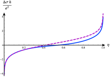
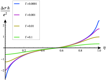
Figure 2: Left panel: Conductivity correction in the absence of block mixing, Eq. (103), as a function of $\eta$ for infinite dephasing time (solid line); sum of the logarithmic WL and WAL asymptotics, Eqs. (105) and (107) (dashed line). Right panel: Conductivity correction for different values of dimensionless dephasing rate $\Gamma$.

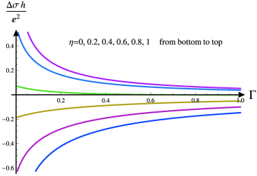
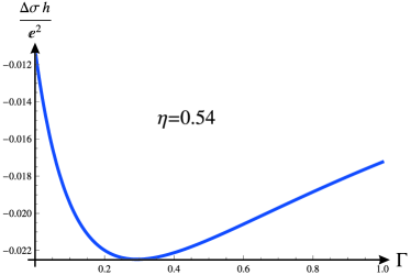
Figure 3: Left panel: Conductivity correction in the absence of block mixing as a function of the dephasing rate for different values of $\eta$. Right panel: Conductivity correction as a function of dephasing rate for $\eta=0.54$.

As discussed above, for $\eta=0$ and $\eta=1$ one of the modes becomes singular (corresponding to $C_{0}$ and $C_{-1},$ respectively). Keeping the singular modes only, one can easily obtain the return probability and the conductivity in vicinities of the points $\eta=0$ and $\eta=1.$ For $\eta\to 0$ we find

$$W(\phi)\approx\frac{1}{2\pi l^{2}}\int\frac{d^{2}\mathbf{Q}}{(2\pi)^{2}}\frac{P_{0}^{3}}{1+\eta^{2}-P_{0}}$$ (104)

and

$$\delta\sigma\approx-\frac{e^{2}}{4\pi^{2}\hbar}\ln\left(\frac{1}{\eta^{2}+\Gamma}\right).$$ (105)

For $\eta\to 1$ we find

$$W(\phi)\approx\frac{e^{-i\phi}}{2\pi l^{2}}\int\frac{d^{2}\mathbf{Q}}{(2\pi)^{2}}\frac{P_{0}^{3}}{1+(1-\eta)^{2}/2\eta-P_{0}-2P_{1}^{2}},$$ (106)

and

$$\delta\sigma\approx\frac{e^{2}}{4\pi^{2}\hbar}\ln\left[\frac{1}{(1-\eta)^{2}/2+\Gamma}\right].$$ (107)

According to Eqs. (105) and (107), the symmetry breaking rates $1/\tau_{A}$ and $1/\tau_{m}$ introduced in Sec. III are equal to

$$1/\tau_{A}=\eta^{2}\gamma\qquad(\eta\ll 1)$$ (108)

and

$$1/\tau_{m}=(1-\eta)^{2}\gamma/2\qquad(1-\eta\ll 1),$$ (109)

respectively.

Using Eqs. (46) and (43), the result (109) for the symmetry-breaking rate $1/\tau_{m}$ in the range of almost linear spectrum ($1-\eta\ll 1$) agrees with the result of Ref. Tkachov11, , where this scale was first identified. In the opposite limit $\eta\to 0$ (which was not analyzed in Ref. Tkachov11, ), the result (108) of the microscopic calculation confirms the estimate of Ref. OGM12, .

The leading logarithmic contributions (105) and (107) are exactly the WL and WAL corrections found in Sec. III from the symmetry analysis for the regimes 2O and 2Sp, respectively. We are now in a position to evaluate corrections to these results. Setting for simplicity $\Gamma=0$ (no dephasing), we get from Eqs. (103) and (99)

$$\delta\sigma\approx\frac{e^{2}}{4\pi^{2}\hbar}\begin{cases}\displaystyle-\ln\frac{1}{\eta^{2}}+\ln 2+(4\ln 2-1)\eta+\frac{5}{2}\eta^{2}\ln\frac{1}{\eta^{2}}+O(\eta^{2}),&\qquad{\rm for}~{}\eta\to 0,\\[8.5359pt] \displaystyle\ln\frac{1}{(1-\eta)^{2}}+3(\ln 2-1)-(1-\eta)-\frac{7}{2}(1-\eta)^{2}\ln\frac{1}{(1-\eta)^{2}}+O[(1-\eta)^{2}],&\qquad{\rm for}~{}\eta\to 1.\end{cases}$$ (110)

The regime $\eta\to 1$ was considered in Ref. Tkachov11, . However, our results for subleading terms in this regime differ from those obtained there. This difference is due to the fact that Ref. Tkachov11, only considered contributions of small momenta $ql\ll 1$. While this is sufficient to get the universal WL and WAL terms (105) and (107), evaluation of the corrections requires taking into account the “ballistic” momenta $ql\gtrsim 1$.

We note that the last term, $\mathcal{O}[(1-\eta)^{2}\ln(1-\eta)],$ in the asymptotics for $\eta\to 1$ in Eq. (110) is, in fact, determined by momenta $ql\ll 1$ and was identified within the diffusive approximation of Ref.  Tkachov11, . However, the numerical coefficient in front of this term in Ref. Tkachov11, , which in our notation would take the form $-(19/8)(1-\eta)^{2}\ln[1/(1-\eta)^{2}]$, differs from the prefactor $-7/2$ in the corresponding term in our Eq. (110). The difference stems from setting $q=0$ everywhere (except for the term $Dq^{2}$ in the denominators of the Cooperon propagators) in the calculation of Ref. Tkachov11, . It is worth emphasizing that the ballistic terms $\mathcal{O}(1)$ and $\mathcal{O}(1-\eta)$ neglected in Ref. Tkachov11, give a much larger contribution in the limit $\eta\to 1$ than this “diffusive-like” term.

The results for arbitrary values of $\eta$ are shown in Figs. 2 and 3. In the left panel of Fig. 2 we plotted the conductivity correction calculated with the use of Eqs. (99) and (103) (solid line) in the absence of dephasing ($\Gamma=0$). The sign of the correction changes with increasing $\eta,$ so that the system undergoes a crossover from the orthogonal to symplectic ensemble as expected. In the same panel we plotted by dashed line the sum of two asymptotes, given by Eqs. (105) and (107), respectively. A deviation of the exact result from the interpolating formula is mostly due to the nonsingular mode related to the eigenvalue $\eta^{2}$ in matrix ${\hat{M}}^{-1}$ given by Eq. (100). As a result, the difference between the solid and dashed lines vanishes in the limit $\eta\to 0$, while yielding a shift $\sim 1$ near $\eta\to 1$. The right panel of Fig. 2 illustrates the crossover at different dephasing rates. In the left panel of Fig. 3 we plotted the conductivity correction as a function of dephasing rate for different $\eta.$ The most interesting feature of these curves is the nonmonotonous dependence of conductivity on $\Gamma$ for $\eta$ close to the point separating localization and delocalization behavior. This feature is emphasized in the right panel of Fig. 3, where dependence of conductivity on dephasing rate is plotted for $\eta=0.54.$ We expect that the conductivity in the 2U symmetry regime (energy $E_{3}$ in Fig. 1) shows an analogous non-monotonous dependence on the magnetic field due to ballistic effects.

IV.3 Block mixing

Let us now briefly analyze the effect of a weak block mixing. As discussed above, on largest scales the mixing leads to a single copy of the symplectic class (1Sp). Below we assume the simplest form of the mixing potential:

$$\hat{V}=V(\mathbf{r})\left[\begin{array}[]{cccc}1&0&0&-\Delta\\ 0&1&\Delta&0\\ 0&\Delta^{*}&1&0\\ -\Delta^{*}&0&0&\end{array}\right],$$ (111)

where $V(\mathbf{r})$ is a short-range potential with the correlation function given by Eq. (44) and $\Delta$ is a parameter responsible for the block mixing. We also assume that $\Delta$ is small and real: $\Delta\ll 1,~{}\Delta=\Delta^{*}.$ The potential Eq. (111) obeys the symmetry: $\hat{V}=\hat{U}\hat{V}^{*}\hat{U}^{-1},$ where

$$\hat{U}=\left[\begin{array}[]{cccc}0&0&-i&0\\ 0&0&0&-i\\ i&0&0&0\\ 0&i&0&0\end{array}\right],~{}~{}\hat{U}\hat{U}^{*}=-1.$$ (112)

The result of the microscopic calculation reads GKO14 :

$$\delta\sigma = \frac{e^{2}}{4\pi^{2}\hbar}\left\{-\ln\left[\Gamma+\frac{(1-\eta)^{2}}{2}\right]\right.$$ (113)

$$- \ln\left[\Gamma+\frac{(1-\eta)^{2}}{2}+2\Delta^{2}\right]+2\ln\big{[}\Gamma+\eta^{2}+2\eta\Delta^{2}\big{]}$$

$$+ \left.\ln\left[\Gamma+\frac{4\Delta^{2}\eta}{1+\eta^{2}}\right]-\ln\Gamma\right\}.$$

We stress that this equation was obtained in the diffusion approximation under the assumption that dimensionless gaps of diffusive modes are small. Hence, though expressions for the last two logarithms in this equation are exact, the explicit form of the first two logarithms is exact only in a vicinity of the point $\eta=1,$ while the third logarithm is exact near the point $\eta=0.$ In this sense, Eq. (113) interpolates between the two limits ($\eta=0$ and $\eta=1$) similarly to Eq. (31) (cf. Fig. 2). Away from the points $\eta=0$ and $\eta=1$ the block mixing in the first three terms of Eq. (113) can be neglected, so that one can use Eq. (103) with Eq. (99) to describe these terms in the crossover range of $\eta$ beyond the diffusive approximation. It is also worth noting that the gap $4\Delta^{2}\eta/(1+\eta^{2})$ in the fourth logarithm is nonzero only when both $\Delta$ and $\eta$ are nonzero, see discussion above Eq. (30).

Introducing the symmetry breaking times $\tau_{m}$, $\tau_{A}$, and $\tau_{\Delta}$ according to

$$\frac{\tau}{\tau_{m}} = \frac{(1-\eta)^{2}}{2},$$ (114)

$$\frac{\tau}{\tau_{A}} = \eta^{2}+2\eta\Delta^{2},$$ (115)

$$\frac{\tau}{\tau_{\Delta}} = \frac{4\Delta^{2}(\eta+2\Delta^{2})}{1+\eta^{2}},$$ (116)

we can rewrite Eq. (113) in a form combining (for $1/\tau_{SO}=0$) Eqs. (26) and (30):

$$\delta\sigma \simeq \frac{e^{2}}{2\pi h}\Bigg{[}-\ln\left(\frac{\tau}{\tau_{\phi}}+\frac{\tau}{\tau_{m}}\right)-\ln\left(\frac{\tau}{\tau_{\phi}}+\frac{\tau}{\tau_{m}}+\frac{\tau}{\tau_{\Delta}}\right)$$ (117)

$$+ 2\ln\left(\frac{\tau}{\tau_{\phi}}+\frac{\tau}{\tau_{A}}\right)+\ln\left(\frac{\tau}{\tau_{\phi}}+\frac{\tau}{\tau_{A}/2+\tau_{\Delta}}\right)$$

$$- \ln\frac{\tau}{\tau_{\phi}}\Bigg{]}.$$

This expression correctly reproduces all singular interference corrections in the whole range $0\leq\eta\leq 1$ provided $\Delta\ll 1$. Note also that for $\eta\ll\Delta^{2}$, Eq. (117) reduces to the conventional expression for the symmetry pattern 2O $\to$ 1Sp with anisotropic spin relaxation (different for in-plane and out-of-plane components) described by $\tau_{||}=\tau_{A}$ and $\tau_{\perp}\simeq\tau_{A}/2=\tau_{||}/2$. In a similar way, one can also include the block mixing described by $1/\tau_{SO}$.

V Weak antilocalization in a quasi-one-dimensional strip

Motivated by recent experiment of Ref. bruene, , we will discuss in this section the magnetoresistance of a quasi-one-dimensional HgTe structure. The magnetotransport measurements in Ref. bruene, were performed on a 2D quantum wells patterned in narrow 1D strips. While the width of the HgTe quantum well is of the order of few nanometers, its lateral width $W$ can be less than hundred nanometers. In such a restricted quasi-1D geometry, boundary conditions play a crucial role for electron transport. Below we analyze possible symmetries of the boundary conditions and ballistic transport effects arising in quasi-1D samples.

V.1 Symmetry breaking mechanism due to boundary scattering

We start by assuming that the boundary does preserve the $s_{z}$-symmetry and the Hamiltonian splits into two independent blocks $h(\mathbf{k})$ and $h^{*}(-\mathbf{k})$ related by the physical TR symmetry. It was demonstrated in Ref. OGM12, that in this case the block-wise TR-symmetry of $h(\mathbf{k})$ is necessarily broken by boundary conditions.

It is well known that a massless Dirac electron cannot be confined by any potential profile due to the Klein tunneling effect. The only way to introduce boundary conditions for a single flavor of Dirac fermions (without block mixing) is to open a gap at the boundary by introducing a large mass in the Hamiltonian. This boundary mass term violates the block-wise symplectic TR symmetry. On a technical level, each boundary scattering event in a Dirac system introduces an additional phase shift in the electron wave function. These scattering phases combine in such a way that the amplitudes of two mutually time-reversed trajectories pick up a relative phase difference $\pi$ for each boundary scattering. Thus the contribution of a trajectory with $N$ boundary scattering events to the conductivity correction contains a factor $(-1)^{N}$. After the summation over all paths with arbitrary $N$, this alternating sign factor kills the singular correction to the conductivity.

More general boundary conditions are possible if the massive BHZ Hamiltonian includes higher-order (quadratic) terms in the $k$ expansion. In particular, the hard-wall boundary conditions, $\psi=0$, are widely used in the literature in this case. The TR symmetry breaking mechanism discussed above is however still effective in this limit provided $E_{F}\gg|m(k_{F})|$. Quadratic terms become important only very close to the boundary, while at a longer distance the dynamics is well described by the linearized Hamiltonian. The hard-wall model effectively reduces to the same infinite mass boundary condition for the problem at these longer scales. An explicit computation of the corresponding scattering states can be found in Ref. OGM12, .

We arrive at the conclusion that the block-wise symplectic TR-symmetry is inevitably broken by the boundary conditions. In a diffusive quasi-1D strip, the edge-induced symmetry-breaking rate reads

$$\frac{1}{\tau_{\text{edge}}}\sim\frac{D}{W^{2}},$$ (118)

where $W$ is the strip width. The time $\tau_{\text{edge}}$ is given by the average time for a particle to propagate diffusively between the edges and “to become aware” of the violation of the block-wise TR symmetry by the boundaries. When the mean free path is longer than the width of the quasi-1D sample, the corresponding symmetry breaking time is given by the typical flight time for ballistic propagation between the two boundaries. The total rate of breaking the block-wise symplectic TR symmetry at $\eta$ close to unity is thus given by $1/\tau_{m}+1/\tau_{\text{edge}}$.

In the opposite limit $\eta\to 0$, when the block-wise TR symmetry is of the orthogonal type, the vanishing of the wave function at the boundary does not lead to the TR symmetry breaking. Indeed, conventional “Schrödinger” particles can be confined by a scalar potential.

Above we have discussed boundary conditions that preserve the $s_{z}$-symmetry. The spin symmetry, however, can be broken at boundaries of a 2D sample if the edges violate the reflection symmetry in $z$-direction. Such edges can be modeled by short-range impurities located near the boundaries. This situation is quite likely for realistic samples. In this case, the only remaining symmetry respected by the edges is the physical symplectic TR symmetry.

V.2 Interference corrections and magnetoresistance in a quasi-1D system

Let us now analyze the interference effects in a quasi-1D geometry, i.e. in a strip of width $W$. We assume a single copy of symplectic class since the block-wise TR symmetry is broken by the boundaries, so that only the patterns 1Sp or 2U $\to$ 1Sp are realized due to the block mixing with no room for 2Sp regime. The magnetoresistance depends on the relations between the width $W$, 2D mean free path $l$, dephasing length $L_{\phi}$, and magnetic length $L_{H}$. We start our analysis with the case of sufficiently weak dephasing $L_{\phi}\gg W$. In the opposite limit, when the dephasing length is shorter than the width of the strip, the WAL correction is given by 2D formulas. For $W\gg L_{\phi}\gg l$ the diffusive results apply, whereas for $W\gg L_{\phi}\lesssim l$ the WAL correction is described by nonuniversal ballistic 2D formulas; the magnitude of the correction is small in this case.

For sufficiently weak magnetic fields, the characteristic length scale at which the interference is suppressed is determined by the condition

$$L_{0}\sim L_{H}^{2}/W.$$ (119)

For such lengths, the area $L_{0}W$ is pierced by one magnetic flux. We assume $L_{0}\gg l$, thus the motion along the strip is diffusive within $L_{0}$. This implies sufficiently weak magnetic field, $L_{H}\gg\sqrt{Wl}$.

When the width of the quasi-1D strip is much larger than the 2D mean free path, $W\gg l$, the correction to the conductance of the strip of length $L$ due to WAL reads:AltshulerAronov81 ; Beenakker ; AA ; AAG

$$\delta G=\frac{e^{2}}{h}\frac{1}{L}\left(\frac{W^{2}}{3L_{H}^{4}}+\frac{1}{L_{\phi}^{2}}\right)^{-1/2}.$$ (120)

Note that this expression assumes a phenomenological ($B$-independent) dephasing length; a more accurate formula including Airy function can be found in Refs. AAK, ; AA, ; AAG, . The difference between the two expressions is of the order of few percent, so that we use the formula (120). The measured correction to the longitudinal conductivity of the 2D array of strips is given by

$$\delta\sigma=\frac{L}{W}\delta G,$$ (121)

neglecting the separation between the strips.

For narrow strips, $W\lesssim l$, the transverse motion is ballistic and the resulting correction is modified,

$$\delta\sigma=\frac{e^{2}}{h}\left(\frac{W^{4}}{3L_{H}^{4}}f(W/l)+\frac{W^{2}}{L_{\phi}^{2}}\right)^{-1/2}.$$ (122)

The function $f(W/l)$ incorporates information about boundary conditions. For diffuse boundaries in the quasi-2D geometry various limiting cases of this function were obtained in Ref. DK, . In a later paper Ref. Beenakker, , this function was computed numerically for both quasi-1D and quasi-2D samples with both mirror and diffuse boundaries. In the limiting case $W\ll l$, analytical expression was also obtained for diffuse boundary conditions.

We represent the quasi-1D results in a closed integral form applicable for all values of $x=W/l$:

$$f_{\text{mirror}}(x) =1-\frac{3}{x^{2}}+\frac{96}{\pi x^{3}}\int ds\,s^{3}\sqrt{1-s^{2}}\tanh\left(\frac{x}{2s}\right)\approx\begin{cases}1,&x\gg 1,\\ \dfrac{186\zeta(5)}{\pi^{5}}\;x\approx 0.63\;x,&x\ll 1,\end{cases}$$ (123a)

$$f_{\text{diffuse}}(x) =1-\frac{4}{\pi x}+\frac{32}{5\pi x^{3}}-\frac{12}{\pi x}\int ds\,s\sqrt{1-s^{2}}e^{-x/s}\left(1+\frac{4s}{x}+\frac{4s^{2}}{x^{2}}\right)\approx\begin{cases}1,&x\gg 1,\\ \dfrac{3x}{2\pi},&x\ll 1.\end{cases}$$ (123b)

These functions are shown in Fig. 4. For $x\equiv W/l\gg 1$, the functions $f(x)$ approach the universal value corresponding to the diffusive result Eq. (120). Ballistic effects partly suppress WAL due to cancellation of magnetic flux piercing purely ballistic trajectories.

Remarkably, the magnitude of the magnetoconductivity peak in quasi-1D geometry is determined only by the ratio of the dephasing length $L_{\phi}$ and the strip width $W$,

$$\delta\sigma(B=0)=\frac{e^{2}}{h}\frac{L_{\phi}}{W}.$$ (124)

Details of transverse ballistic motion, encoded in the function $f(W/l)$, are relevant only for the width of the peak.

Let us now consider the case of a relatively weak block mixing described by $L_{SO}$. Then the conductivity correction takes the form

$$\delta\sigma = \frac{e^{2}}{h}\left[\left(\frac{W^{4}}{3L_{H}^{4}}f(W/l)+\frac{W^{2}}{L_{\phi}^{2}}\right)^{-1/2}\right.$$ (125)

$$- \left.\left(\frac{W^{4}}{3L_{H}^{4}}f(W/l)+\frac{W^{2}}{L_{\phi}^{2}}+\frac{W^{2}}{L_{SO}^{2}}\right)^{-1/2}\right].$$

For a strong block mixing this equation reproduces the 1Sp result (122), while in the opposite limit of weak mixing the conductivity correction gets strongly suppressed as illustrated in Fig. 5.

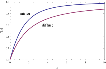
Figure 4: Functions $f_{\text{mirror}}(x)$ and $f_{\text{diffuse}}(x)$ defined in Eqs. (123).

Figure 5: Conductivity correction in a quasi-1D strip of HgTe, Eq. (125), for $W/l\gg 1$, $W/L_{\phi}=0.2,$ and different values of the block-mixing length: $W/L_{SO}=2,\,1,\,0.5,\,0.3,\,0.2,\,0.1,\,0.05$ from top to bottom.

VI Summary and discussion

To summarize, we have reviewed manifestations of quantum interference in conductivity of 2D HgTe structures. A symmetry analysis yields a rich “phase diagram” describing regimes with different types of one-loop quantum interference correction (WL, WAL, no correction). We have supplemented the symmetry analysis by a microscopic calculation of the quantum interference contribution to the conductivity. This approach allows us also to calculate the behavior of the conductivity in the crossover regimes and beyond the diffusive approximation. We have also discussed symmetry breaking mechanisms and the quantum interference correction in a quasi-1D (strip) geometry.

Figure 6: Schematic illustration of the magnetoresistivity $\rho_{xx}(B)$ on a linear-logarithmic scale for energies $E_{1}\ldots E_{5}$ from the right panel of Fig. 1. The numbers denote the prefactors $\alpha=(\pi h/e^{2})\partial\sigma/\partial\ln\tau_{H}$ (here $\tau_{H}=L_{H}^{2}/D$) of the logarithmic magnetoresistivity.

The common way to explore the quantum interference (WL or WAL) experimentally is to measure the magnetoresistivity $\rho_{xx}(B)$ in a transverse magnetic field $B$. Each of the symmetry-breaking patterns discussed in Sec. II then translates into a succession of regions of magnetic field with corresponding signs and prefactors of the low-field magnetoresistivity, see Fig.6.

Let us now discuss available experimental data in context of the above theoretical findings. In Refs. kvon, ; minkov, the low-field magnetoresistivity was investigated in 2D HgTe samples both in the case of normal (thin QWs) and inverted (thick QWs) band ordering. For both types of samples a weak positive magnetoresistivity was observed in the lowest magnetic fields $B$. This behavior can clearly be attributed to WAL. The coefficient in front of $(e^{2}/\pi h)\ln\tau_{H}$ (where $\tau_{H}=L_{H}^{2}/D$) was found to be consistent with 1/2, as expected for the 1Sp regime. In higher magnetic fields, a crossover to negative magnetoresistance was observed that could be presumably attributed to WL. Such a behavior corresponds, in our terminology, to the $2\,{\rm O}\to 1\,{\rm Sp}$ symmetry pattern (characteristic for systems with relatively small carrier concentration, see regimes E₁ and E₂ in Fig. 6)footnote_ballistic . For inverted structures with high carrier concentrations, Ref. minkov, observed only positive magnetoresistance consistent with regimes E₄ and E₅ of Fig. 6.

In a recent work bruene the magnetoresistance of a HgTe structure patterned in an array of quasi-1D strips was experimentally studied. The WAL behavior was observed both for normal-gap and inverted-gap structures in the whole range of magnetic fields and gate voltages. This is consistent with the 1Sp behavior as expected from the above theory in the quasi-1D regime. Indeed, boundaries of the strips break the block-wise TR symmetry, as has been shown in Sec. V.1. Furthermore, diffuse boundary scattering due to short-range edge irregularities is favorable for the violation of the $z\to-z$ symmetry at the boundary, which breaks down the spin symmetry, yielding the 1Sp regime. In addition, the block mixing arises also due to the BIA, see Ref. Qi11, , and due to short-range impurities located within the quantum well. The difference in the magnitude of the effect for normal-gap and inverted-gap setups observed in Ref. bruene, can be possibly related to a stronger block mixing in the inverted case (cf. Fig. 5) and/or stronger dephasing in the normal case. A stronger block-mixing in the inverted case might possibly be attributed to the higher probability of having irregularities (background short-range impurities or edge roughness) breaking the $z\to-z$ symmetry of the sample within a thicker QW (inverted band ordering) as compared to a thin QW (normal band ordering).

Finally, it is worth emphasizing that, while we have focussed on HgTe/HgCdTe quantum wells, the above analysis is expected to be applicable to a broader class of structures with Dirac-type spectrum, including, in particular, InAs/GaSb structures Liu08 ; Du .

VII Acknowledgments

We are grateful to C. Brüne, A. Germanenko, E. Hankiewicz, E. Khalaf, G. Minkov, L. Molenkamp, M. Titov, and G. Tkachov for useful discussions. The work was supported by DFG-RFBR within DFG SPP “Semiconductor spintronics”, by DFG-SPP 1666, by RFBR, by grant FP7-PEOPLE-2013-IRSES of the EU network InterNoM, by GIF, and by BMBF.

References

- (1) M. Z. Hasan and C. L. Kane, Rev. Mod. Phys. 82, 3045 (2010).
- (2) X.-L. Qi and S.-C. Zhang, Rev. Mod. Phys. 83, 1057 (2011).
- (3) B.A. Bernevig, T.L. Hughes, and S.-C. Zhang, Science 314, 1757 (2006).
- (4) M. König, S. Wiedmann, C. Brüne, A. Roth, H. Buhmann, L.W. Molenkamp, X.-L. Qi, and S.-C. Zhang, Science 318, 766 (2007).
- (5) C. L. Kane and E. J. Mele, Phys. Rev. Lett. 95, 146802 (2005); ibid. 95, 226801 (2005).
- (6) L. Fu and C. L. Kane, Phys. Rev. B 76, 045302 (2007); L. Fu, C.L. Kane, and E.J. Mele, Phys. Rev. Lett. 98, 106803 (2007).
- (7) D. Hsieh, D. Qian, L. Wray, Y. Xia, Y.S.Hor, R.J. Cava, and M.Z.Hasan, Nature 452, 7190 (2008).
- (8) M. König, H. Buhmann, L.W. Molenkamp, T. Hughes, C.-X. Liu, X.-L. Qi, and S.-C. Zhang, J. Phys. Soc. Jpn. 77, 031007 (2008); A. Roth, C. Brüne, H. Buhmann, L.W. Molenkamp, J. Maciejko, X.-L. Qi, and S.-C. Zhang, Science 325, 294 (2009).
- (9) C. Liu, T.L. Hughes, X.-L. Qi, K. Wang, and S.-C. Zhang, Phys. Rev. Lett. 100, 236601 (2008).
- (10) I. Knez, Rui-Rui Du, and G. Sullivan, Phys. Rev. Lett. 107, 136603 (2011); L. Du, I. Knez, G. Sullivan, and Rui-Rui Du, arXiv:1306.1925.
- (11) P. M. Ostrovsky, I. V. Gornyi, and A. D. Mirlin, Phys. Rev. Lett. 105, 036803 (2010).
- (12) G. Tkachov and E. M. Hankiewicz, Phys. Rev. B 84, 035444 (2011).
- (13) P. M. Ostrovsky, I. V. Gornyi, and A. D. Mirlin, Phys. Rev. B 86, 125323 (2012).
- (14) V. Krueckl and K. Richter, Semicond. Sci. Technol. 27, 124006 (2012).
- (15) E. McCann, K. Kechedzhi, V.I. Fal’ko, H. Suzuura, T. Ando, and B.L. Altshuler, Phys. Rev. Lett. 97, 146805 (2006); K. Kechedzhi, E. McCann, V.I. Fal’ko, H. Suzuura, T. Ando, and B. L. Altshuler, Eur. Phys. J. Special Topics 148, 39 (2007).
- (16) I. L. Aleiner and K. B. Efetov, Phys. Rev. Lett. 97, 236801 (2006).
- (17) P.M. Ostrovsky, I.V. Gornyi, and A.D. Mirlin, Phys. Rev. B 74, 235443 (2006).
- (18) M.O. Nestoklon, N.S. Averkiev, and S.A. Tarasenko, Solid State Comm. 151, 1550 (2011).
- (19) I. Garate and L. Glazman, Phys. Rev. B 86, 035422 (2012).
- (20) E.J. König, P.M. Ostrovsky, I.V. Protopopov, I.V. Gornyi, I.S. Burmistrov, and A.D. Mirlin, Phys. Rev. B 88, 035106 (2013).
- (21) G.M. Minkov, A.V. Germanenko, O.E. Rut, A.A. Sherstobitov, S.A. Dvoretski, and N.N. Mikhailov, Phys. Rev. B 85, 235312 (2012); Phys. Rev. B 88, 045323 (2013).
- (22) E.B. Olshanetsky, Z.D. Kvon, G.M. Gusev, N.N. Mikhailov, S.A. Dvoretsky, and J.C. Portal, JETP Lett. 91, 347 (2010); D. A. Kozlov, Z. D. Kvon, N. N. Mikhailov, and S. A. Dvoretsky, JETP Lett. 96, 730 (2013).
- (23) M. Mühlbauer, A. Budewitz, B. Büttner, G. Tkachov, E.M. Hankiewicz, C. Brüne, H. Buhmann, and L.W. Molenkamp, Phys. Rev. Lett. 112, 146803 (2014).
- (24) D.G. Rothe, R.W. Reinthaler, C.-X. Liu, L.W. Molenkamp, S.-C. Zhang, and E.M. Hankiewicz, New J. Phys. 12, 065012 (2010).
- (25) R. Winkler, Spin-Orbit Coupling Effects in Two-Dimensional Electron and Hole Systems, Springer Tracts in Modern Physics, Volume 191, (Springer, Berlin, 2003).
- (26) A similar role is played by disorder that acts differently on E and H subbands. In the rotated basis used in Sec. III, the corresponding term in the Haniltonian is proportional to , similarly to , and can be regarded as a random mass term. In the regime of an almost linear spectrum, , such disorder would lead to an additional contribution to . On the other hand, when the chemical potential is located near the band bottom, , such type of disorder does not yield additional symmetry breaking and only contributes to the elastic scattering time .
- (27) B. L. Altshuler and A. G. Aronov, in Electron-electron interactions in disordered conductors, edited by A. L. Efros and M. Pollak (Elsevier, 1985), p. 1.
- (28) S. Chakravarty and A. Schmid, Physics Reports 140, 4 (1986).
- (29) I. L. Aleiner, B. L. Altshuler, and M. E. Gershenzon, Waves Random Media 9, 201 (1999).
- (30) In fact, this question is more subtle and the term requires special attention. It results in an ultraviolet logarithmic divergency (coming from large momenta ) of the return probability This divergency leads to ultraviolet renormalization aleiner-efetov of the key problem parameters (such as ) and will not be discussed here. By default, we assume that all parameters of the problem are already renormalized and that
- (31) A. P. Dmitriev, V. Yu. Kachorovskii, and I. V. Gornyi, Phys. Rev. B 56, 9910 (1997).
- (32) I. V. Gornyi, V. Yu. Kachorovskii, and P.M. Ostrovsky, Phys. Rev. B. 90, 085401 (2014).
- (33) V.K. Dugaev and D.E. Khmelnitskii, Sov. Phys. JETP 59, 1038 (1984).
- (34) B. L. Altshuler and A. G. Aronov, JETP Lett. 33, 499 (1981).
- (35) C. W. J. Beenakker and H. van Houten, Phys. Rev. B 38, 3232 (1988).
- (36) B.L. Altshuler, A.G. Aronov, and D.E. Khmelnitskii, J. Phys. C 15, 7367 (1982).
- (37) A weak negative magnetoresistance in relatively strong fields may also arise in the E3 regime of Fig. 6 due to ballistic effects, cf. Fig. 3 (right panel).