Collective modes in a Dirac insulator with short range interactions

Abstract

We study a Haldane model with nearest neighbor interactions. We find one-dimensional like collective modes arising due to the interplay of pseudo-spin and valley degrees of freedom. In the large band gap or moderate interaction limit, these excitations are low energy modes lying in the band gap. The dispersion relations are qualitatively different in trivial insulator phase and Chern insulator phase, thus can be used to identify the topology of the Haldane model with the bulk property. We also discuss how to detect these modes in cold atom systems. An abelian gauge theory will emerge when a physical current-current interaction is introduced to the Haldane model or the Kane-Mele model.

I Introduction

The discovery of graphene gn opens the door of studying Dirac fermions in condensed matter systems. Topological insulator ti1 ; ti2 is a novel state of matter hosting gappless Dirac fermions on the surface and can be described by a massive Dirac equation in the bulk. The collective excitations in these systems attract much interests both theoretically and experimentally. The plasmon in graphene under various conditions has been discussed extensively va ; wun ; hw ; gan ; gon ; pya ; sarma ; ande ; sode ; stefan and observed experimentally nature1 . Plasmons are collective modes that are usually absent in an insulator. It’s shown that due to the interplay between Dirac and Schrödinger fermions stefan , plasmons appear in 2D topological insulator, e.g., Hg(Cd)Te quantum wells. These modes are also sensitive to the bulk topology stefan ; zhou . The spin-momentum locking effect on the surface of a 3D strong topological insulator induces a curious effect: density fluctuations induce spin fluctuations and vice versa and this gives the spin-plasmon zhang . The observation of Dirac plasmons in topological insulators is reported recently natp1 . Ref. stauber reviews the recent progress of plasmons in graphene and topological insulator.

In this paper we study the collective modes in a Haldane model hald , which has been realized in the optical lattice experiments very recently 1406 . It is natural to consider short range interactions in the optical lattice, so the collective modes are analogous with the zero sound in a neutral fermi liquid. Plasmons in gapped graphene have been studied in Ref. pya where the density-density correlation is calculated. Surprisingly, we find the interplay of pseudo-spin and valley degrees of freedom gives a new phenomenon: one dimensional-like collective modes that are not reported before emerge. The underline lattice $C_{3}$ symmetry is broken by the quantum anomaly. These modes are qualitatively different in topological trivial phase and non-trivial phase and can be used to identify the topology of Haldane model.

Random phase approximation (RPA) is widely used to study the collective modes and its validity is established in graphene sarmar . Here we use a different form of RPA nagaosa , i.e., we derive the one-loop effective field theory of the collective modes. Around a single valley, the effective theory is equivalent to a Maxwell-Chern-Simons theory pp ; frad ; kondo . In pp the authors eliminated a valley with larger gap. However, we find the contribution of the heavier Dirac point is as large as the lighter one up to the lowest order works . If we consider the contributions of both valleys properly, the effective theory is no longer equivalent to a Maxwell-Chern-Simons theory. Combining the contributions from two Dirac points, there is no gauge symmetry anymore, while new effects arise. We find one-dimensional collective modes emerge in both topological trivial (trivial insulator) and topological nontrivial (Chern insulator) cases. The behavior of the collective modes is qualitatively different: The wave vector is perpendicular to the direction of the two Dirac points in a trivial insulator while it is along the direction of the two Dirac points in a Chern insulator. The gaps of the modes are also different. When the band gap is large and the interaction is not too small, both modes can lie in the band gap. The in-gap collective modes have been observed in the topological Kondo insulator $\mathrm{SmB_{6}}$ smb_e . These modes originate from the strong interactions smb_t . In our case, the in-gap modes appear for weak or moderate interactions and strong enough interactions will induce a Mott transition mottran .

Recently, the quantum simulation of the dynamic gauge theories attracts a lot of interests in the cold atom and other systems buch ; kapit ; zohar ; zoharc ; ban ; zoharcr ; mac ; tag ; bane ; zoharprl ; tagl ; zohara ; wiese . Most researches focused on simulating the lattice gauge theories hon ; orl ; chand . Ref. pp provides a new idea although, in our opinion, the authors missed the effect of the heavier Dirac fermion. We thus construct a model in which the gauge theories do emerge. Taking account of the rapid development of cold atom experiments, we hope the model can be realized in the near future.

The rest of this paper is organized as follows. In Sec. II we introduce the model and derive the low energy effective Lagrangian of the model. In Sec. III we present the dispersion relations of the collective modes in both trivial insulator and Chern insulator phases. We then discuss how to detect them in cold atom systems. A different interaction is needed to get an emergent gauge theory and we briefly discuss this in Sec. IV. Finally, a conclusion is given in Sec. V.

II Model and method

The Haldane model on honeycomb lattice hald ; 1406 is governed by the following Hamiltonian:

$$H_{0}=-\sum_{\langle ij\rangle_{1}}t_{ij}c^{\dagger}_{i}c_{j}-\sum_{\langle ij\rangle_{2}}\lambda_{ij}e^{i\phi_{ij}}c_{i}^{\dagger}c_{j}+\Delta\sum_{i}(-1)^{i}c^{{\dagger}}_{i}c_{i},$$ (1)

where $c^{{\dagger}}_{i}$ ($c_{i}$) is the fermion creation (annihilation) operator on site $i$, $t_{ij}$ is the nearest hopping amplitude and $\lambda_{ij}$ is the next-to-nearest neighbor one. $\phi_{ij}$ is the directed phase defined along the arrows in Fig.1 and when $|\phi_{ij}|\neq 0,\pi$, it will break the time reversal symmetry. $2\Delta$ is the onsite energy difference of sublattices and it breaks inversion symmetry. Time reversal symmetry breaking and inversion symmetry breaking terms both give a band gap. However, the gaps are different in topological nature. As a result, varying $\Delta/\lambda$ induces a topological phase transition from a Chern insulator to a trivial insulator hald . Although important, Haldane model seems unrealistic in materials. Fortunately, the rapid progress in cold atom experimental techniques gives new possibilities. In a recent experiment 1406 , Haldane model has been realized in a time-modulated optical lattice. Experimentally, $t_{ij}$ and $\lambda_{ij}$ are bond-dependent and $\phi_{ij}$ is controlled by the modulation phase. Our results don’t rely on the details of these parameters and we will take $t_{ij}=t$, $\lambda_{ij}=\lambda$ and $|\phi_{ij}|=\pi/2$ for simplification.

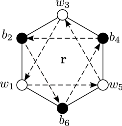
Figure 1: Haldane model on honeycomb lattice. Black and white points mark the sublattice. Arrows denote the positive phase hopping. r is the center of the plaquette.

There are 3 nearest neighbors on the honeycomb lattice (set the lattice constant to be $1$),

$$\mathbf{b}_{1}=(\frac{1}{2\sqrt{3}},\frac{1}{2}),\mathbf{b}_{2}=(\frac{1}{2\sqrt{3}},-\frac{1}{2}),\mathbf{b}_{3}=(-\frac{1}{\sqrt{3}},0),$$ (2)

and 6 next-to-nearest neighbors,

$$\mathbf{a}_{1}=(\frac{\sqrt{3}}{2},-\frac{1}{2}),\mathbf{a}_{2}=(0,1),\mathbf{a}_{3}=(\frac{\sqrt{3}}{2},\frac{1}{2}),$$

$$\mathbf{a}_{4}=(-\frac{\sqrt{3}}{2},\frac{1}{2}),\mathbf{a}_{5}=(0,-1),\mathbf{a}_{6}=(-\frac{\sqrt{3}}{2},-\frac{1}{2}).$$ (3)

Now we rewrite the Hamiltonian $H_{0}$ in the momentum space,

$$H_{0}=-t\sum_{\mathbf{k}}((\sum_{i=1}^{3}e^{i\bf{k}\cdot\mathbf{b}_{i}})b_{\mathbf{k}}^{\dagger}w_{\mathbf{k}}+h.c.)$$

$$+\sum_{\bf{k}}[\Delta-2\lambda(\sin(\sqrt{3}k_{x}/2+k_{y}/2)-\sin(k_{y})-$$

$$\sin(\sqrt{3}k_{x}/2-k_{y}/2))](b^{\dagger}_{\mathbf{k}}b_{\mathbf{k}}-w^{\dagger}_{\mathbf{k}}w_{\mathbf{k}}).$$ (4)

where we label the two sublattices by $b$ and $w$. Now let us consider the low energy behavior around the two independent Dirac points $\vec{K}$ and $-\vec{K}$, with $\vec{K}=(0,\frac{4\pi}{3})$. Here we take $\hbar=1$. The mass gap at $K_{\pm}$ is $m_{\pm}c^{2}=\Delta\pm 3\sqrt{3}\lambda$ and $c=\frac{\sqrt{3}}{2}t$ is the Fermi velocity and we take $c=1$ in the following; At half-filling, the Fermi level lies in the gap. In the long wavelength limit, Eq. (II) can be approximated around $K_{\pm}$ to the linear order of the momentum $p$

$$H_{0}\approx\sum_{p,v}\psi^{\dagger}_{p,v}{\cal H}_{0}(p,v)\psi_{p,v},$$ (5)

where $v=\pm$ is the valley index labeling the Dirac points $K_{\pm}$, $\psi_{p,v}=(b_{pv},w_{pv})^{T}$ is the two component fermion spinor near the Dirac point $K_{v}$ and $b,w$ label the two sub-lattices. The Hamiltonian ${\cal H}_{0}(p,v)$ is a $2\times 2$ matrix given by

$${\cal H}_{0}(p,v)=vp_{y}\tau^{x}-p_{x}\tau^{y}-m_{v}\tau^{z}.$$ (6)

Notice the $v$ before $p_{y}$. Because of this sign, the chiralities of the Dirac points are the same if the signs of $m_{\pm}$ are different. This gives a simple way to calculate the Chern number: $\nu=\frac{1}{2}[{\rm sgn}(m_{+})-{\rm sgn}(m_{-})]$. When $\nu=0$, the system is a trivial insulator; when $\nu=\pm 1$, it’s a Chern insulator. As we will show below, $v$ also plays an important role in the effective theory of collective modes.

We consider the nearest neighbor Hubbard interaction

$$H_{int}=U\sum_{\langle ij\rangle_{1}}n_{i}n_{j}.$$ (7)

In order to take the correct continuum limit, we rewrite the interaction Eq. (7) by summing over the plaquettes (see Fig. 1), i.e.,

$$H_{int} = \frac{U}{2}\sum_{\langle bw\rangle\in\rm plaq}(n_{w_{1}}n_{b_{2}}+n_{b_{2}}n_{w_{3}}+n_{w_{3}}n_{b_{4}}$$ (8)

$$+n_{b_{4}}n_{w_{5}}+n_{w_{5}}n_{b_{6}}+n_{b_{6}}n_{w_{1}}).$$

Now we approximate $n_{i}$ by its value at the center of the plaquette (denote as ${\bf r}$), for example,

$$n_{w_{1}} \approx n_{w}({\bf r})-\frac{\sqrt{3}}{3}(\frac{\sqrt{3}}{2}\partial_{x}n_{w}({\bf r})+\frac{1}{2}\partial_{y}n_{w}({\bf r})),$$ (9)

$$n_{b_{2}} \approx n_{b}({\bf r})-\frac{\sqrt{3}}{3}(\frac{\sqrt{3}}{2}\partial_{x}n_{b}({\bf r})-\frac{1}{2}\partial_{y}n_{b}({\bf r})).$$ (10)

Therefore after some arithmetics, Eq. (7) becomes,

$$H_{int}=\frac{g^{2}}{2}\sum_{{\bf r}}(6n_{b}({\bf r})n_{w}({\bf r})+\frac{\sqrt{3}}{2}\nabla n_{b}({\bf r})\cdot\nabla n_{w}({\bf r})),$$ (11)

where $g^{2}=U$. In the continuum limit, we drop the second term. The disappearance of the first order terms is guaranteed by the lattice symmetry.

To make further progress we write the density-density interaction in the suggestive way:

$$6n_{b}n_{w}=(n_{b}+n_{w})^{2}-(c^{{\dagger}}_{b}c_{w}+c^{{\dagger}}_{w}c_{b})^{2}-(-ic^{{\dagger}}_{b}c_{w}+ic^{{\dagger}}_{w}c_{b})^{2}.$$

We have omitted the $n_{b}+n_{w}$ terms since they can be absorbed into chemical potential.

Now we decouple the interaction Eq. (11) using the following Hubbard-Stratonovich transformation:

$$\exp\biggl{\{}-\frac{ig^{2}}{2}\int dtd^{2}r~{}6n_{b}(\mathbf{r})n_{w}(\mathbf{r})\biggr{\}}$$

$$=\int\mathcal{D}a_{\mu}\exp\biggl{\{}i\int dtd^{2}r(\frac{1}{2}a_{\mu}a^{\mu}+gj_{\mu}a^{\mu})\biggr{\}},$$ (12)

with $\mu=0,1,2$ and $j_{0}=n_{b}+n_{w}$, $j_{1}=-ic^{{\dagger}}_{b}c_{w}+ic^{{\dagger}}_{w}c_{b}$ and $j_{2}=-c^{{\dagger}}_{b}c_{w}-c^{{\dagger}}_{w}c_{b}$. In Eq. (12) we use Einstein’s summation convention and the metric is $g^{\mu\nu}=diag(1,-1,-1)$. We then approximate the 3-‘current’ by $j_{\mu}\approx\sum_{v}j_{\mu v}$ with $j_{\mu v}$ defined near $K_{v}$, i.e.,

$$j_{0v}=\psi^{\dagger}_{v}({\bf r})\psi_{v}({\bf r}),$$

$$j_{1v}=\psi^{\dagger}_{v}({\bf r})\tau^{y}\psi_{v}({\bf r}),$$ (13)

$$j_{2v}=-\psi^{\dagger}_{v}({\bf r})\tau^{x}\psi_{v}({\bf r}).$$

It’s crucial to notice that the ‘current’ $j_{2}=j_{2,+}+j_{2,-}$ is not the physical current. The physical current should be $j_{2,phy}=j_{2,+}-j_{2,-}$ because the coefficient of $p_{y}$ has an opposite sign around the two Dirac points, see Eq. (6). This simple fact leads to some interesting physical phenomena.

Now we can write down the low energy effective Lagrangian as:

$${\cal L} = \sum_{v}(\bar{\psi}_{v}(t,{\bf r})(i{\not}\partial_{v}+m_{v})\psi_{v}(t,{\bf r})$$ (14)

$$+gj_{\mu}a^{\mu}+\frac{1}{2}a_{\mu}a^{\mu}),$$

where $\bar{\psi}_{v}=\psi^{\dagger}_{v}\gamma^{0}_{v}$ and ${\not}\partial_{v}=\gamma^{\mu}_{v}\partial_{\mu}$, $\gamma^{0}_{v}=\tau^{z}$, $\gamma^{1}_{v}=i\tau^{x}$, $\gamma^{2}_{v}=vi\tau^{y}$, $\partial_{\mu}=(\partial_{t},\partial_{x},\partial_{y})$. We can rewrite the ‘current’ in terms of the gamma matrices: $j_{v}^{0/1}=\bar{\psi}_{v}\gamma_{v}^{0/1}\psi_{v}$ and $j^{2}_{v}=v\bar{\psi}_{v}\gamma_{v}^{2}\psi_{v}$. Notice that the effective Lagrangian (14) is rotationally invariant. This is the result of the long wavelength limit. If the higher orders beyond the linear approximation of the wave vector are included, the symmetry should be reduced to the lattice $C_{3}$ point group symmetry.

III collective modes and experimental implications

The physical meanings of $a_{0}$, $a_{x}$ and $a_{y}$ are the charge and pseudo-spin densities. We don’t decouple in $s^{z}$ channel because the density fluctuations only couple to $s^{x}$ and $s^{y}$ components of pseudo-spin zhang . To discuss the properties of the collective modes we integrate over the fermions. The one-loop result has the form $\mathcal{L}_{\mathrm{eff}}=\frac{1}{2}(a^{2}-g^{2}a^{\mu}\Pi_{\mu\nu}a^{\nu})$. $\Pi_{\mu\nu}$ is nothing but the bare susceptibility tensor, this verifies the equivalence between our approach and RPA.

Up to $1/|m_{\pm}|$ order, the one-loop result is given by (see Appendix. A)

$$\mathcal{L}_{\mathrm{eff}} = \frac{g^{2}}{8\pi}\mathrm{sgn}(m_{+})\varepsilon^{\mu\nu\rho}a_{\mu}\partial_{\nu}a_{\rho}-\frac{g^{2}}{24\pi|m_{+}|}F^{\mu\nu}_{a}F_{a,\mu\nu}$$ (15)

$$-\frac{g^{2}}{8\pi}\mathrm{sgn}(m_{-})\varepsilon^{\mu\nu\rho}b_{\mu}\partial_{\nu}b_{\rho}-\frac{g^{2}}{24\pi|m_{-}|}F^{\mu\nu}_{b}F_{b,\mu\nu}$$

$$+\frac{1}{2}a^{2},$$

where $F_{a,\mu\nu}=\partial_{\mu}a_{\nu}-\partial_{\nu}a_{\mu}$, $F_{b,\mu\nu}=\partial_{\mu}b_{\nu}-\partial_{\nu}b_{\mu}$ and $b_{0}=-a_{0}$, $b_{1}=-a_{1}$ and $b_{2}=a_{2}$. The first line of Eq. (15) is the contribution of $K_{+}$ and the second line comes from $K_{-}$. Two Chern-Sinoms terms corresponding to two Dirac points come from the $m_{\pm}$-zeroth order contributions and are the quantum anomalies of the Dirac fermion. We emphasize $a_{\mu}$ and $b_{\mu}$ are not independent and will discuss its physical results soon.

We make some observations about the contribution of a single Dirac point: There is a constraint of $a_{\mu}$ fields which is a direct result of the equation of motion. The physical reason of the constraint is that the charge density only couples to the transverse component of spin density zhang . The effective action around a single Dirac point becomes a Maxwell-Chern-Simons theory after a dual transformation pp ; frad ; kondo . In pp , the authors eliminate the Dirac point with a larger mass. However, up to the lowest order, the contribution of a Dirac point only dependents on the sign of its mass (see Eq. (15)), thus there is no way to get rid of the effect of the heavier Dirac fermion, as emphasized by Haldane hald . Notice that $a_{\mu}$ and $b_{\mu}$ have the same magnitude but the sign may be the same or opposite. This leads to two remarkable results: (i) The rotational symmetry is broken by the quantum anomaly in the one loop approximation. This means that the underline lattice $C_{3}$ symmetry is also broken if the high order expansions are considered. (ii) The effective theory is no longer a gauge theory because of the cancellation of some of the components of the $a_{\mu}$ field. However, this also means that the $a_{\mu}$ field cannot be completely canceled even in the topological trivial case. In the following we study the dispersions of the collective modes $a_{\mu}$ in the topological trivial and nontrivial phases.

For $\mathrm{sgn}(m_{+})=\mathrm{sgn}(m_{-})$, i.e., the trivial insulator case, the collective modes are dynamical in the lowest order approximation so we can omit the $1/|m_{\pm}|$ corrections. The pole of Green’s function of $a_{\mu}$ gives the following dispersion relation:

$$\omega^{2}=p_{x}^{2}+m_{A}^{2},$$ (16)

where $m_{A}=2\pi/g^{2}$. This dispersion is one-dimensional like. $p_{x}$ is the direction perpendicular to the vector that connects the two Dirac points, so it’s physically distinct from $p_{y}$. When $m_{A}<\mathrm{min}(|m_{+}|,|m_{-}|)$, this mode lies in the band gap and will not decay to single particle excitations. Let the band gap be $\Delta_{t}$ and recover the ‘speed of light’ $c$, the in-gap condition becomes $U\Delta_{t}>2\pi c^{2}$ which can be fulfilled in the large band gap or the strong interaction limit. A strong enough interaction will induce a Mott transition mottran . However, on the one hand, the critical interaction of Mott transition is of the order of band width mottran . On the other hand, the band gap can be tuned in cold atom systems. We thus expect that the in-gap modes can be observed experimentally.

For $\mathrm{sgn}(m_{+})=-\mathrm{sgn}(m_{-})$, i.e., the Chern insulator case, to get the dispersion of the collective modes one have to consider the $1/|m_{\pm}|$ corrections. We then find two dispersions around the Dirac points

$$\omega^{2}\approx 6\pi M/g^{2}+p_{x}^{2}+\beta p_{y}^{2},$$ (17)

$$\omega^{2}\approx 6\pi M/g^{2}+\alpha g^{2}Mp_{y}^{2}+p^{2}_{x},$$ (18)

with $M=\frac{|m_{+}m_{-}|}{|m_{+}|+|m_{-}|}$, and $\alpha,\beta$ are dependent on $|m_{+}|,|m_{-}|$ and are of order 1. These modes can also lie in the band gap. Let the band gap be $\Delta_{n}$ and $|m_{+}|=|m_{-}|$, the in-gap condition is $U\Delta_{n}>3\pi c^{2}$. Comparing this condition with the one in topological trivial case, we find that for the same $U$ and $c$, the band gap $\Delta_{n}$ should be larger than $\Delta_{t}$ to get the in-gap modes. Generally speaking, this means that the gap of the in-gap collective modes in a Chern insulator is larger than that in a trivial insulator. Since we are considering the large band gap limit, $M>>1$, the dispersion Eq. (18) is one-dimensional like and can be approximated as

$$\omega^{2}=6\pi M/g^{2}+\alpha g^{2}Mp_{y}^{2}.$$ (19)

This mode is the characteristic mode in the Chern insulator phase: it’s one-dimensional like with large velocity.

Now we get the main results of this paper: we find that in an insulator with Dirac points, the lattice point group symmetry may be broken by the quantum anomaly and there are one-dimensional like collective modes. These bulk modes also reveal the topology of the insulator: in the large band gap limit, the gap of collective modes of a Chern insulator is larger than that of a trivial insulator and both modes can lie in the band gap. What is more, the dispersion of the collective modes in a Chern insulator is along a given direction, say, connecting the two Dirac points while in a trivial insulator it is perpendicular to that direction. We are not aware of collective modes with these properties.

Our predictions can be examined in cold atom experiments. The collective modes can by measured through Bragg scattering. In the Bragg scattering process, two laser beams with 3-momentum difference $q_{\mu}=k_{1\mu}-k_{2\mu}$ are sent to the trapped cold atom gases on the optical lattice. The illuminated cold atom system responds to this perturbation with a density fluctuation $H^{\prime}=(V/2)(\delta j_{0}({\bf q})e^{iq_{0}t}+h.c.)$. The atoms then absorb a momentum after the Bragg scattering. The rate of the momentum transfer can be measured by the time of flight images and be related to the dynamic structure factor by $d{\bf P}/dt=2\pi{\bf q}(V/2)^{2}[S(q_{\mu})-S(-q_{\mu})]\propto(1-e^{-\beta q_{0}})S(q_{\mu})\propto\mathrm{Im}(\chi_{q})$ where ${\bf P}$ is the total momentum of the atoms and $\chi_{q}$ is the density-density correlation bragg . Because the interaction is relatively weak, the heating arising from the interaction is negligible and then $\partial{\bf P}/dt$ can be evaluated at zero temperature, i.e., $\propto S(q_{\mu})$. It may be hard to detect the pseudospin density correlation directly, however, the density correlation is enough for our purpose. In our case, the density-density correlation is just the correlation of $a_{0}$ and can be calculated easily.

For a trivial insulator,

$$\langle a_{0,-q}a_{0,q}\rangle=2\frac{\omega^{2}-m_{A}^{2}}{\omega^{2}-p_{x}^{2}-m_{A}^{2}},$$

with $m_{A}=2\pi/g^{2}$, this gives

$$\mathrm{Im}(\chi_{q})=2\pi p^{2}_{x}\delta(\omega^{2}-p_{x}^{2}-m_{A}^{2}).$$ (20)

For a Chern insulator, we consider two limits, i.e., $|m_{+}|=|m_{-}|\equiv M$ and $|m_{+}|>>|m_{-}|\equiv M$.

For $|m_{+}|=|m_{-}|\equiv M$, $a_{y}$ mode is decoupled from $a_{0}$ and $a_{x}$ and the dispersion of $a_{y}$ mode is

$$\omega^{2}=m_{A,c}^{2}+p^{2}_{x},$$

with $m_{A,c}^{2}=3\pi M/g^{2}$. This dispersion is along $p_{x}$ direction with a small ‘velocity’. The one-dimensional nature of this mode is due to the special parameter. What’s more, this mode cannot be detected by density-density correlation. On the other hand, the characteristic mode can be revealed from the density-density correlation:

$$\langle a_{0,-q}a_{0,q}\rangle=\frac{2m^{2}_{A,c}(\omega^{2}-p^{2}_{y}-m^{2}_{A,c})}{(\omega^{2}-E^{2}_{\mathbf{p}})(p^{2}_{y}+m^{2}_{A,c})},$$

where $E^{2}_{\mathbf{p}}=m^{2}_{A,c}+p^{2}_{y}+p^{2}_{x}+\frac{1}{4\pi^{2}}\frac{m^{4}_{A,c}g^{4}}{m^{2}_{A,c}+p^{2}_{y}}p^{2}_{y}\approx m^{2}_{A,c}+\frac{m^{2}_{A,c}g^{4}}{4\pi^{2}}p^{2}_{y}$, and we have

$$\mathrm{Im}(\chi_{q})\approx\frac{g^{4}m^{2}_{A,c}}{2\pi}p^{2}_{y}\delta(\omega^{2}-E^{2}_{\mathbf{p}}).$$ (21)

For $|m_{+}|>>|m_{-}|\equiv M$,

$$\langle a_{0,-q}a_{0,q}\rangle\approx\frac{2(\omega^{2}-m^{2}_{A,c})(\omega^{2}-p^{2}_{x}-p^{2}_{y}-m^{2}_{A,c})}{(\omega^{2}-p^{2}_{x}-m^{2}_{A,c})(\omega^{2}-m^{2}_{A,c}-\frac{m^{2}_{A,c}g^{4}}{4\pi^{2}}p^{2}_{y})},$$

here $m^{2}_{A,c}=6\pi M/g^{2}$. There are two modes and are all one-dimensional like due to the special parameter. The characteristic mode is along the $p_{y}$ direction. Along the $p_{y}$ direction the structure factor has the same form as Eq. (21):

$$\mathrm{Im}(\chi_{p_{x}=0})\approx\frac{g^{4}m^{2}_{A,c}}{2\pi}p^{2}_{y}\delta(\omega^{2}-m^{2}_{A,c}-\frac{m^{2}_{A,c}g^{4}}{4\pi^{2}}p^{2}_{y}).$$ (22)

Finally, we would like to point out that although the $C_{3}$ symmetry is broken, the coordinate axes $x$ and $y$ are arbitrarily chosen. In practice, it should be pinned by various imperfects, impurities and other circumstances.

IV emergent gauge theory

In this section, we construct an interaction such that gauge theory emerges. As we have emphasized several times in the previous sections, the ‘current’ $j_{2}=j_{2,+}+j_{2,-}$ is not the physical current. The physical current should be

$$j_{2,phy}=j_{2,+}-j_{2,-}.$$

To get the emergent gauge field, we simply replace $j_{2}$ by $j_{2,phy}$ in Eq. (14), then the model becomes a Thirring model thir ; thirc . We construct a lattice interaction in Appendix B. After integrating over the fermions the effective Lagrangian becomes (See Appendix A):

$$\mathcal{L}_{\mathrm{eff}} = \frac{g^{2}\nu}{4\pi}\varepsilon^{\mu\nu\rho}a_{\mu}\partial_{\nu}a_{\rho}-\frac{g^{2}}{24\pi M}F^{\mu\nu}F_{\mu\nu}+\frac{1}{2}a^{2},$$ (23)

where $\nu=\frac{1}{2}(\mathrm{sgn}(m_{+})-\mathrm{sgn}(m_{-}))$ is the Chern number, $M=\frac{|m_{+}m_{-}|}{|m_{+}|+|m_{-}|}$ and $F_{\mu\nu}=\partial_{\mu}a_{\nu}-\partial_{\nu}a_{\mu}$. When $\nu=0$, this is a massive Maxwell theory (Proca theory); when $\nu\neq 0$, it’s equivalent to a Chern-Simons-Maxwell theory after a dual transformation kondo . The mass of Proca theory is $6\pi M/g^{2}$ while the mass of Chern-Simons-Maxwell theory is $2\pi/g^{2}+\mathcal{O}(1/M)$. The mass of the Proca theory can hardly be tuned small because we require $M$ to be large to get the effective action. Hence, it is impossible to discuss the confinement effect poly . The mass of Chern-Simons-Maxwell theory can be tuned small if the interaction is large or the ‘speed of light’ is small.

Kane-Mele model KM ; KM1 is essentially two copies of Haldane model related by time reversal symmetry and can also be realized by the same technique in Ref. 1406 . The collective modes discussed in Sec. III also appear in Kane-Mele model with short range interactions KMH such as $U\sum_{\langle ij\rangle_{1};\sigma}n_{i\sigma}n_{j\sigma}$. What is more, it is possible to reach to the confinement limit if the interaction is of physical current-current type. In this case, due to introducing of the spin degrees of freedom, we get a mutual Chern-Simons theory (up to $\mathcal{O}(1/|m_{\pm}|)$):

$$\mathcal{L}_{\mathrm{eff}} = \frac{g^{2}\nu_{\sigma}}{4\pi}\varepsilon^{\mu\nu\rho}a_{\sigma\mu}\partial_{\nu}a_{\sigma\rho}+\frac{1}{2}a^{2}_{\sigma},$$ (24)

where $a_{\sigma}$ is the collective modes of spin-$\sigma$ fermions and $\nu_{\uparrow}=-\nu_{\downarrow}$, as is required by time reversal symmetry. Let $A_{\mu}=a_{\mu\uparrow}-a_{\mu\downarrow}$, In terms of $A_{\mu}$ and $a_{\mu\uparrow}$, the Lagrangian ${\cal L}_{\mathrm{eff}}$ becomes,

$$\mathcal{L}_{\mathrm{eff}} = \frac{1}{2}a^{\mu}_{\uparrow}a_{\mu\uparrow}+\frac{1}{2}(\frac{8\pi^{2}}{\alpha^{2}}A^{2}-\frac{4\sqrt{2}\pi}{\alpha}A_{\mu}a^{\mu}_{\uparrow}+a^{\mu}_{\uparrow}a_{\mu\uparrow})$$ (25)

$$-\sqrt{2}\epsilon^{\mu\nu\rho}a_{\mu\uparrow}\partial_{\nu}A_{\rho}+\frac{2\pi}{\alpha}\epsilon^{\mu\nu\rho}A_{\mu}\partial_{\nu}A_{\rho}.$$

Now let us integrate out the $a_{\mu\uparrow}$ field, we get the effective Lagrangian,

$${\cal L}_{eff}=-\frac{F^{\mu\nu}F_{\mu\nu}}{4}+\frac{1}{2}m_{A}^{2}A^{\mu}A_{\mu},$$ (26)

with $F_{\mu\nu}=\partial_{\mu}A_{\nu}-\partial_{\nu}A_{\mu}$ and $m_{A}=2\pi/g^{2}$. In this case, it is possible to pursue the massless Maxwell limit and study the confinement effect in the continuum gauge theory experimentally.

Notice that the rotational symmetry is kept for the physical current-current interactions.

V Conclusions

We have investigated the collective modes in a Dirac insulator, i.e., Haldane model with short range interaction. We have shown one-dimensional excitations emerge due to the interplay between the valley and the pseudo-spin degrees of freedom. For those linear excitations, the $C_{3}$ symmetry is broken by quantum anomaly. The qualitative behavior of the modes is quite different in topological trivial phase and nontrivial phase thus can be used to identify the phase of the Haldane model with its bulk property. We also discuss how to detect these modes in cold atom experiments. The interplay between Dirac fermions and Schrödinger fermions may lead to new phenomena and will be studied in a future work, where the effects of lattice will be considered as well. We also construct the interactions that lead to emergent gauge theories of the collective modes, e.g., Proca theory and Chern-Simons-Maxwell theory.

Appendix A Effective field theory of collective modes

In this appendix we show how to get Eq. (15) from Eq. (14).

$$\mathcal{L}=\mathcal{L}_{+}+\mathcal{L}_{-}+\frac{1}{2}a^{2},$$

where $\mathcal{L}_{\pm}$ is the Lagrangian around Dirac point $K_{\pm}$:

$\mathcal{L_{+}}=\bar{\psi}_{+}(i\gamma^{0}\partial_{0}+i\gamma^{1}\partial_{1}+i\gamma^{2}\partial_{2}+m_{+})\psi_{+}+ga_{\mu}\bar{\psi_{+}}\gamma^{\mu}\psi_{+},$

$\mathcal{L_{-}}=\bar{\psi}_{-}(i\gamma^{0}\partial_{0}+i\gamma^{1}\partial_{1}-i\gamma^{2}\partial_{2}+m_{-})\psi_{-}+ga_{\mu}\bar{\psi_{-}}\gamma^{\mu}\psi_{-}.$

Note that the fermions around the two Dirac points are decoupled and can be integrated out independently. We can integrate over $\psi_{+}$ and the result is well known frad ; kondo ; jackiw , in large mass limit we get the first line of Eq. (15)

For the $\psi_{-}$ fermions, let $\gamma^{\prime 0}=-\gamma^{0}$, $\gamma^{\prime 1}=-\gamma^{1}$, $\gamma^{\prime 2}=\gamma^{2}$, $b^{0}=-a^{0}$, $b^{1}=-a^{1}$, $b^{2}=a^{2}$, then $\mathcal{L}_{-}$ can be written as

$\mathcal{L_{-}}=-\bar{\psi}_{-}(i\gamma^{\prime\mu}\partial_{\mu}-m_{-})\psi_{-}+gb_{\mu}\bar{\psi}_{-}\gamma^{\prime\mu}\psi_{-}.$

Integrating over $\psi_{-}$, $\mathcal{L}_{-}$ gives the second line of Eq. (15).

To get a gauge theory, $a_{2}$ should couple to the physical current $j_{2,+}-j_{2,-}$. $\mathcal{L}_{+}$ is unchanged while $\mathcal{L}_{-}$ becomes:

$$\mathcal{L_{-}} = \bar{\psi}_{-}(i\gamma^{0}\partial_{0}+i\gamma^{1}\partial_{1}-i\gamma^{2}\partial_{2}+m_{-})\psi_{-}$$

$$+ga_{0}\bar{\psi}_{-}\gamma^{0}\psi_{-}+ga_{1}\bar{\psi}_{-}\gamma^{1}\psi_{-}-ga_{2}\bar{\psi_{-}}\gamma^{2}\psi_{-}$$

$$= -\bar{\psi}_{-}(i\gamma^{\prime\mu}\partial_{\mu}-m_{-})\psi_{-}-ga_{\mu}\bar{\psi}_{-}\gamma^{\prime\mu}\psi_{-}.$$

Integrating over $\psi_{+}$ and $\psi_{-}$ we get Eq. (23).

Appendix B Current-current interaction on lattice

To get the effective gauge theory, the interaction terms should be:

$$a_{0}(\bar{\psi}_{+}\gamma^{0}\psi_{+}+\bar{\psi}_{-}\gamma^{0}\psi_{-})+a_{1}(\bar{\psi}_{+}\gamma^{1}\psi_{+}+\bar{\psi}_{-}\gamma^{1}\psi_{-})+$$

$$a_{2}(\bar{\psi}_{+}\gamma^{2}\psi_{+}-\bar{\psi}_{-}\gamma^{2}\psi_{-}).$$

As we have shown in the main text, the first term comes from the nearest neighbor interaction $n_{i}n_{j}$. To get a lattice version of the last two terms, we first regularize the second term as, e.g.:

$$a_{1}(\bar{\psi}_{+}\gamma^{1}\psi_{+}+\bar{\psi}_{-}\gamma^{1}\psi_{-})=a_{1}(\psi^{{\dagger}}_{+}\sigma^{y}\psi_{+}+\psi^{{\dagger}}_{-}\sigma^{y}\psi_{-})$$

$$\sim a_{1,\mathbf{q}}\cos(k_{1})\psi^{{\dagger}}_{\mathbf{k}}\sigma^{y}\psi_{\mathbf{k-q}}$$

$$=a_{1,\mathbf{q}}\cos(k_{1})(-ic^{{\dagger}}_{b,\mathbf{k}}c_{w,\mathbf{k-q}}+ic^{{\dagger}}_{w,\mathbf{k}}c_{b,\mathbf{k-q}})$$

$$=\frac{a_{1,\mathbf{q}}}{2}\sum_{i}(-ic^{{\dagger}}_{b,i}c_{w,i\pm\mathbf{a}_{1}}+ic^{{\dagger}}_{w,i}c_{b,i\pm\mathbf{a}_{1}})e^{i\mathbf{q}\cdot(\mathbf{R}_{i}\pm\mathbf{a}_{1})},$$

where $i$ denotes the unit cell and $\mathbf{a}_{1}$ is one of the six next-to-nearest neighbors. And similarly for the third term,

$$a_{2}(\bar{\psi}_{+}\gamma^{2}\psi_{+}-\bar{\psi}_{-}\gamma^{2}\psi_{-})=a_{2}(\psi^{{\dagger}}_{+}\sigma^{x}\psi_{+}-\psi^{{\dagger}}_{-}\sigma^{x}\psi_{-})$$

$$\sim a_{2,\mathbf{q}}\sin(k_{1})\psi^{{\dagger}}_{\mathbf{k}}\sigma^{x}\psi_{\mathbf{k-q}}$$

$$=a_{2,\mathbf{q}}\sin(k_{1})(c^{{\dagger}}_{b,\mathbf{k}}c_{w,\mathbf{k-q}}+c^{{\dagger}}_{w,\mathbf{k}}c_{b,\mathbf{k-q}})$$

$$=\frac{a_{2,\mathbf{q}}}{2i}\sum_{i}\pm(c^{{\dagger}}_{b,i}c_{w,i\pm\mathbf{a}_{1}}+c^{{\dagger}}_{w,i}c_{b,i\pm\mathbf{a}_{1}})e^{i\mathbf{q}\cdot(\mathbf{R}_{i}\pm\mathbf{a}_{1})}.$$

Integrating over $a_{1}$ and $a_{2}$ fields, we get the corresponding lattice interaction:

$$c^{{\dagger}}_{b,i}c_{b,i+\mathbf{a}_{1}}c^{{\dagger}}_{w,i+\mathbf{a}_{1}}c_{w,i}+h.c..$$

There are different ways to regularize the current $j_{2,phy}$ and the resultant lattice interactions are also different.

References

- (1) A. K. Geim and K. S. Novoselov, Nat. Mater. 6, 183 (2007).
- (2) M. Z. Hasan and C. L. Kane, Rev. Mod. Phys. 82, 3045 (2010).
- (3) X. L. Qi and S. C. Zhang, Rev. Mod. Phys. 83, 1057 (2011).
- (4) Oskar Vafek, Phy. Rev. Lett 97, 266406 (2006).
- (5) B.Wunsch, T. Stauber, F. Sols, and F. Guinea, New Journal of Physics 8, 318 (2006).
- (6) E. H. Hwang and S. Das Sarma, Phys. Rev. B 75, 205418 (2007).
- (7) S. Gangadharaiah, A. M. Farid, and E. G. Mishchenko, Phy. Rev. Lett 100, 166802 (2008).
- (8) J. González and E. Perfetto, Phy. Rev. Lett 101, 176802 (2008).
- (9) P. K. Pyatkovskiy, J. Phys.: Condens. Matter 21 025506 (2009).
- (10) I. Sodemann and M. M. Fogler Phys. Rev. B 86, 115408 (2012).
- (11) S. Das Sarma and Qiuzi Li, Phy. Rev. B 87, 235418 (2013).
- (12) David R Andersen and Hassan Raza, J. Phys.: Condens. Matter 25 045303 (2013).
- (13) S. Juergens, P. Michetti, and B. Trauzettel, Phys. Rev. Lett. 112, 076804 (2014).
- (14) Long Ju, Baisong Geng, Jason Horng, Caglar Girit, Michael Martin, Zhao Hao, Hans A. Bechte, Xiaogan Liang, Alex Zettl, Y. Ron Shen, and Feng Wang, Nat. Nanotechnol. 6, 630 (2011).
- (15) H. R. Chang, J. Zhou, H. Zhang, and Y. Yao, Phys. Rev. B 89, 201411(R) (2014).
- (16) S. Raghu, S. B. Chung, X. L. Qi and S. C. Zhang, Phys. Rev. Lett. 104, 116401 (2010).
- (17) P. Di Pietro, M. Ortolani, O. Limaj, A. Di Gaspare, V. Giliberti, F. Giorgianni, M. Brahlek, N. Bansal, N. Koirala, S. Oh, P. Calvani, and S. Lupi, Nat. Nanotechnol. 8, 556 (2013).
- (18) T. Stauber, J. Phys.: Condes. Matter 26,123201 (2014).
- (19) F. D. M. Haldane, Phys. Rev. Lett. 61, 2015 (1988).
- (20) G. Jotzu, M. Messer, R. Desbuquois, M. Lebrat, T. Uehlinger, D. Greif and T. Esslinger, Nature 515, 237 (2014)
- (21) Johannes Hofmann, Edwin Barnes and S. Das Sarma, Phys. Rev. Lett. 113, 105502 (2014)
- (22) N. Nagaosa, Quantum Field Theory in Strongly Correlated Electronic Systems, (Springer, 1999).
- (23) G. Palumbo and J. K. Pachos, Phys. Rev. Lett. 110, 211603 (2013).
- (24) E. Fradkin and F. A. Schaposnik, Phys. Lett. B 338, 253 (1994).
- (25) Kei-Ichi Kondo, Prog. Theor. Phys. 94, 899 (1995).
- (26) X. Luo, Y. P. Lan, Y. Yu and L. Liang (unpublished).
- (27) W. T. Fuhrman, J. Leiner, P. Nikolić, G. E. Granroth, M. B. Stone, M. D. Lumsden, L. DeBeer-Schmitt, P. A. Alekseev, J.-M. Mignot, S. M. Koohpayeh, P. Cottingham, W. Adam Phelan, L. Schoop, T. M. McQueen, and C. Broholm, arXiv:1407.2647.
- (28) W. T. Fuhrman and P. Nikolic, Phys. Rev. B 90, 195144 (2014).
- (29) Christopher N. Varney, Kai Sun, Marcos Rigol, and Victor Galitski, Phys. Rev. B 82, 115125 (2010).
- (30) H. P. Buchler, M. Hermele, S. D. Huber, M. P. A. Fisher, and P. Zoller, Phys. Rev. Lett. 95, 040402 (2005).
- (31) E. Kapit and E. Mueller, Phys. Rev. A 83, 033625 (2011).
- (32) E. Zohar and B. Reznik, Phys. Rev. Lett. 107, 275301(2011).
- (33) E. Zohar, J. I. Cirac, and B. Reznik, Phys. Rev. Lett. 109, 125302 (2012).
- (34) D. Banerjee, M. Dalmonte, M. Müller, E. Rico, P. Stebler, U. J. Wiese, and P. Zoller, Phys. Rev. Lett. 109,175302 (2012).
- (35) E. Zohar, J. I. Cirac, and B. Reznik, Phys. Rev. Lett. 110,055302 (2013).
- (36) D. Marcos, P. Rabl, E. Rico, and P. Zoller, Phys. Rev. Lett. 111, 110504 (2013).
- (37) L. Tagliacozzo, A. Celi, A. Zamora, and M. Lewenstein, Ann. Phys. 330, 160 (2013).
- (38) D. Banerjee, M. Bögli, M. Dalmonte, E. Rico, P. Stebler, U. J. Wiese, P. Zoller, Phys. Rev. Lett. 110, 125303 (2013).
- (39) E. Zohar, J. I. Cirac, and B. Reznik, Phys. Rev. Lett. 110, 125304 (2013).
- (40) L. Tagliacozzo, A. Celi, P. Orland, M.W. Mitchell, and M. Lewenstein, Nature Communications 4, 2615 (2013).
- (41) E. Zohar, J. I. Cirac, and B. Reznik, Phys. Rev. A 88, 023617 (2013).
- (42) For more references, see, e.g., U. J. Wiese, Ann. der Phys. 525, 777 (2013).
- (43) D. Horn, Phys. Lett. B 100, 149 (1981).
- (44) P. Orland and D. Rohrlich, Nucl. Phys. B 338, 647 (1990).
- (45) S. Chandrasekharan and U.-J Wiese, Nucl. Phys. B 492, 455 (1997).
- (46) A. Brunello, F. Dalfovo, L. Pitaevskii, S. Stringari, and F. Zambelli, Phys. Rev. A 64, 063614 (2001).
- (47) W. Thirring, Annals. Phys. 3, 91 (1958).
- (48) J. I. Cirac, P. Maraner, and J. K. Pachos, Phys. Rev. Lett 105, 190403 (2010).
- (49) A. M. Polyakov, Nucl. Phys. B 120, 429 (1977).
- (50) C. L. Kane and E. J. Mele, Phys. Rev. Lett. 95, 146802 (2005).
- (51) C. L. Kane and E. J. Mele, Phys. Rev. Lett. 95, 226801 (2005).
- (52) Kane-Mele model with Hubbard interaction has been studied extensively, see e.g., S. Rachel and K. Le Hur, Phys. Rev. B 82, 075106 (2010), D. Zheng, G. M. Zhang and C. Wu, Phys. Rev. B 84, 205121 (2011), J. Wen, M. Kargarian, A. Vaezi, and G. A. Fiete, Phy. Rev. B 84, 235149 (2011), C. Griset and C. Xu, Phys. Rev. B 85, 045123 (2012), A. Vaezi, M. Mashkoori and M. Hosseini, Phy. Rev. B 85, 195126 (2012), W. Wu, S. Rachel, W. M. Liu and K. Le Hur, Phy. Rev. B 85, 205102 (2012), M. Hohenadler, Z. Y. Meng, T. C. Lang, S. Wessel, A. Muramatsu and F. F. Assaad, Phys. Rev. B 85, 115132 (2012).
- (53) S. Deser, R. Jackiw and S. Templeton, Annals. Phys. 140, 372 (1982).