Almost the Best of Three Worlds: Risk, Consistency and Optional Stopping for the Switch Criterion in Nested Model Selection

Abstract

We study the switch distribution, introduced by Van Erven et al. (2012), applied to model selection and subsequent estimation. While switching was known to be strongly consistent, here we show that it achieves minimax optimal parametric risk rates up to a $\log\log n$ factor when comparing two nested exponential families, partially confirming a conjecture by Lauritzen (2012) and Cavanaugh (2012) that switching behaves asymptotically like the Hannan-Quinn criterion. Moreover, like Bayes factor model selection but unlike standard significance testing, when one of the models represents a simple hypothesis, the switch criterion defines a robust null hypothesis test, meaning that its Type-I error probability can be bounded irrespective of the stopping rule. Hence, switching is consistent, insensitive to optional stopping and almost minimax risk optimal, showing that, Yang’s (2005) impossibility result notwithstanding, it is possible to ‘almost’ combine the strengths of AIC and Bayes factor model selection.

and

t1Research supported by the Netherlands Organization for Scientific Research. t2This research was supported by NWO VICI Project 639.073.04.

1 Introduction

We consider the following standard model selection problem, where we have i.i.d. observations $X_{1},\ldots,X_{n}$ and we wish to select between two nested parametric models,

$$\mathcal{M}_{0}=\left\{p_{\mu}\mid\mu\in M_{0}\right\}\quad\text{ and }\quad\mathcal{M}_{1}=\{p_{\mu}\mid\mu\in M_{1}\}.$$ (1.1)

Here the $X_{i}$ are random vectors taking values in some set ${\cal X}$, $M_{1}\subseteq\mathbb{R}^{m_{1}}$ for some $m_{1}>0$ and ${\cal M}_{0}=\{p_{\mu}:\mu\in M_{0}\}\subset\mathcal{M}_{1}$ represents an $m_{0}$-dimensional submodel of $\mathcal{M}_{1}$, where $0\leq m_{0}<m_{1}$. We may thus denote $\mathcal{M}_{0}$ as the ‘simple’ and $\mathcal{M}_{1}$ as the ‘complex’ model. We will assume that $\mathcal{M}_{1}$ is an exponential family, represented as a set of densities on ${\cal X}$ with respect to some fixed underlying measure, so that $p_{\mu}$ represents the density of the observations, and we take it to be given in its mean-value parameterization. As the notation indicates, we require, without loss of generality, that the parameterizations of ${\cal M}_{0}$ and ${\cal M}_{1}$ coincide, that is $M_{0}\subset M_{1}$ is itself a set of $m_{1}$-dimensional vectors, the final $m_{1}-m_{0}$ components of which are fixed to known values. We restrict ourselves to the case in which both $M_{1}$ and the restriction of $M_{0}$ to its first $m_{0}$ components are products of open intervals.

Most model selection methods output not just a decision $\delta(X^{n})\in\{0,1\}$, but also an indication $r(X^{n})\in{\mathbb{R}}$ of the strength of evidence, such as a $p$-value or a Bayes factor. As a result, such procedures can often be interpreted as methods for hypothesis testing, where ${\cal M}_{0}$ represents the null model and ${\cal M}_{1}$ the alternative; a very simple example of our setting is when the $X_{i}$ consist of two components $X_{i}\equiv(X_{i1},X_{i2})$, which according to $\mathcal{M}_{1}$ are independent Gaussians whereas under $\mathcal{M}_{2}$ they can have an arbitrary bivariate Gaussian distribution and hence can be dependent. Since we allow $\mathcal{M}_{0}$ to be a singleton, this setting also includes some very simple, classical yet important settings such as testing whether a coin is biased (${\cal M}_{0}$ is the fair coin model, ${\cal M}_{1}$ contains all Bernoulli distributions).

We consider three desirable properties of model selection methods: (a) optimal worst-case risk rate of post-model selection estimation (with risk measured in terms of squared error loss, squared Hellinger distance, Rényi or Kullback-Leibler divergence); (b) consistency, and, (c), for procedures which also output a strength of evidence $r(X^{n})$, whether the validity of the evidence is insensitive to optional stopping under the null model. We evaluate the recently introduced model selection criterion $\delta_{\text{sw}}$ based on the switch distribution (Van Erven et al., 2012) on properties (a), (b) and (c).

The switch distribution, introduced by Van Erven et al., (2007), was originally designed to address the catch-up phenomenon, which occurs when the best predicting model is not the same across sample sizes. The switch distribution can be interpreted as a modification of the Bayesian predictive distribution. It also has an MDL interpretation: if one corrects standard MDL approaches (Grünwald, 2007) to take into account that the best predicting method changes over time, one naturally arrives at the switch distribution. Lhéritier and Cazals (2015) describe a successful practical application for two-sample sequential testing, related to the developments in this paper but in a nonparametric context. We briefly give the definitions relevant to our setting in Section 2; for all further details we refer to Van Erven et al. (2012) and E in the Appendix.

When evaluating any model selection method, there is a well-known tension between properties (a) and (b) above: the popular AIC method (Akaike, 1973) achieves the minimax optimal parametric rate of order $1/n$ in the problem above, but is inconsistent; the same holds for the many popular model selection methods that asymptotically tend to behave like AIC, such as $k$-fold (for fixed $k$) and leave-one-out-cross-validation, the bootstrap and Mallow’s $C_{p}$ in linear regression (Efron, 1986; Shao, 1997; Stone, 1977). On the other hand, BIC (Schwarz, 1978) is consistent in the sense that for large enough $n$, it will select the smallest model containing the ‘true’ $\mu$; but it misses the minimax parametric rate by a factor of $\log n$. The same holds for traditional Minimum Description Length (MDL) approaches (Grünwald, 2007) and Bayes factor model selection (BFMS) (Kass and Raftery, 1995), of which BIC is an approximation. This might lead one to wonder if there exists a single method that is optimal in both respects. A key result by Yang (2005) shows that this is impossible: any consistent method misses the minimax optimal rate by a factor $g(n)$ with $\lim_{n\rightarrow\infty}g(n)=\infty$.

In Section 4.2 we show that, Yang’s result notwithstanding, the switch distribution allows us to get very close to satisfying property (a) and (b) at the same time, at least in the problem defined above (Yang’s result was shown in a nested linear regression rather than our exponential family context, but it does hold in our exponential family setting as well; see the discussion at the end of Section 3.3). We prove that in our setting, the switch model selection criterion $\delta_{\text{sw}}$ (a) misses the minimax optimal rate only by an exceedingly small $g_{\text{sw}}(n)\asymp\log\log n$ factor (Theorem 1). Property (b), strong consistency, was already shown by Van Erven et al. (2012). The factor $g_{\text{sw}}(n)\asymp\log\log n$ is an improvement over the extra factor resulting from Bayes factor model selection, which has $g_{\text{\sc bfms}}(n)\asymp\log n$. Indeed, as discussed in the introduction of van Erven et al. (2012), the catch-up phenomenon that the switch distribution addresses is intimately related to the rate-suboptimality of Bayesian inference. Van Erven et al. (2012) show that, while model selection based on switching is consistent, sequential prediction based on model averaging with the switching method achieves minimax optimal cumulative risk rates in general parametric and nonparametric settings, where the cumulative risk at sample size $n$ is obtained by summing the standard, instantaneous risk from $1$ to $n$. In contrast, in nonparametric settings, standard Bayesian model averaging typically has a cumulative risk rate that is larger by a $\log n$ factor. Using the cumulative risk is natural in sequential prediction settings, but Van Erven et al. (2012) left open the question of how switching would behave for the more standard, instantaneous risk. In contrast to the cumulative setting, we cannot expect to achieve the optimal rate here by Yang’s (2005) result, but it is interesting to see that switching gets so close.

We now turn to the third property, robustness to optional stopping. While consistency in the sense above is an asymptotic and even somewhat controversial notion (see Section 6), there exists a nonasymptotic property closely related to consistency that, while arguably more important in practice, has received relatively little attention in the recent statistical literature. This is property (c) above, insensitivity to optional stopping. In statistics, the issue was thoroughly discussed, yet never completely resolved, in the 1960s; nowadays, it is viewed as a highly desirable feature of testing methods by, for example, psychologists; see (Wagenmakers, 2007; Sanborn and Hills, 2014). In particular, it is often argued (Wagenmakers, 2007) that the fixed stopping rule required by the classical Neyman-Pearson paradigm severely and unnecessarily restricts the application domain of hypothesis testing, invalidating much of the $p$-values reported in the psychological literature. Approximately 55% of psychologists admitted in a survey to deciding whether to collect more data after looking at their results to see if they were significant (John et al., 2012). We analyze property (c) in terms of robust null hypothesis tests, formally defined in Section 5. A method defines a robust null hypothesis test if (1) it outputs evidence $r(X^{n})$ that does not depend on the stopping rule used to determine $n$, and (2) (some function of) $r(X^{n})$ gives a bound on the Type-I error that is valid no matter what this stopping rule is. Standard (Neyman-Pearson) null hypothesis testing and tests derived from AIC-type methods are not robust in this sense. For example, such tests cannot be used if the stopping rule is simply unknown, as is often the case when analyzing externally provided data — but this is just the tip of an iceberg of problems with nonrobust tests. For an exhaustive review of such problems we refer to Wagenmakers (2007) who builds on, amongst others, Berger and Wolpert (1988) and Pratt (1962).

Now, as first noted by Edwards et al. (1963), in simple versus composite testing (i.e. when $\mathcal{M}_{0}$ is a singleton), the output of BFMS, the Bayes factor, does provide a robust null hypothesis test. This is one of the main reasons why for example, in psychology, Bayesian testing is becoming more and more popular (Dienes, 2011; Andrews and Baguley, 2012), even among ‘frequentist’ researchers (Sanborn and Hills, 2014). Our third result, in Section 5, shows that the same holds for the switch criterion: if $\mathcal{M}_{0}$ is a singleton, so that the problem (1.1) reduces to a simple versus composite hypothesis test, then the evidence $r(X^{n})$ associated with the switching criterion has the desired robustness property as well and thus in this sense behaves like the Bayes factor method. The advantage, from a frequentist point of view, of switching as compared to Bayes is then that switching is a lot more sensitive: our risk rate results directly imply that the Type II error $(1-\text{power})$ of the switch criterion goes to $0$ as soon as, at sample size $n$, the distance between the ‘true’ distribution $\mu_{1}$ and the null model, i.e. $\inf_{\mu\in M_{0}}\|\mu-\mu_{1}\|^{2}_{2}$ is of order $(\log\log n)/n$; for Bayes factor testing, in order for the Type-II error to reach $0$, this distance must be of order $(\log n)/n$ (this was informally recognized by Lhéritier and Cazals (2015), who reported substantially larger power of switching as compared to the Bayes factor method in a sequential two-sample testing setting).

Thus, for singleton ${\cal M}_{0}$, switching gives us ‘almost the best of three worlds’: minimax rate optimality up to a $\log\log n$ factor (in contrast to BFMS), consistency (in contrast to AIC-type methods) and nonasymptotic insensitivity to optional stopping (in contrast to standard Neyman-Pearson testing) in combination with a small Type-II error. For composite ${\cal M}_{0}$, we show in Section 5 that nonasymptotic robustness to optional stopping still holds, albeit only in a much weaker sense — thus pointing towards an obvious goal for future work, discussed in Section 6: can we modify the switch distribution so as to get full optional stopping robustness also for composite ${\cal M}_{0}$?

Organization

This paper is organized as follows. The switch criterion is introduced in Section 2. In Section 3, we provide some preliminaries: we list the loss/risk functions for which our result holds, describe the sets in which the truth is assumed to lie, and discuss the tension between consistency and rate-optimality. Suitable post-model-selection estimators to be used in combination with the switch criterion are introduced in Section 4, after which our main result on the worst-case risk of the switch criterion is stated. We also go into the relationship between the switch criterion and the Hannan-Quinn criterion in that section. In Section 5 we define robust null hypothesis tests, give some examples, and show that testing by switching has the desired nonasymptotic robustness to optional stopping; in constrast, AIC does not satisfy such a property at all and the Hannan-Quinn criterion only satisfies an asymptotic analogue. We also provide some simulations that illustrate our results. Section 6 provides some additional discussion and ideas for future work. All proofs are given in the Appendix.

Notations and Conventions

We use $x^{n}=x_{1},\ldots,x_{n}$ to denote $n$ observations, each taking values in a sample space $\mathcal{X}$. For a set of parameters $M$, $\mu\in M$, and $x\in\mathcal{X}$, $p_{\mu}(x)$ invariably denotes the density or mass function of $x$ under the distribution $\mathbb{P}_{\mu}$ of random variable $X$, taking values in $\mathcal{X}$. This is extended to $n$ outcomes by independence, so that $p_{\mu}(x^{n}):=\prod_{i=1}^{n}p_{\mu}(x_{i})$ and ${\mathbb{P}}_{\mu}(X^{n}\in A_{n})$, abbreviated to ${\mathbb{P}}_{\mu}(A_{n})$, denotes the probability that $X^{n}\in A_{n}$ for $X^{n}=X_{1},\ldots,X_{n}$ i.i.d. $\sim{\mathbb{P}}_{\mu}$. Similarly, ${\mathbb{E}}_{\mu}$ denotes expectation under ${\mathbb{P}_{\mu}}$. As is customary, we write $a_{n}\asymp b_{n}$ to denote $0<\lim_{n\to\infty}\inf a_{n}/b_{n}\leq\lim_{n\to\infty}\sup a_{n}/b_{n}<\infty$. For notational simplicity we assume throughtout this paper that whenever we refer to a sample size $n$, then $n\geq 3$ to ensure that $\log\log n$ is defined and positive.

Throughout the text, we refer to standard properties of exponential families without always giving an explicit reference; all desired properties can be found, in precise form, in (Barndorff-Nielsen, 1978) and, on a less formal level, in (Grünwald, 2007, Chapter 18,19).

2 Model Selection by Switching

The switch distribution (Van Erven et al., 2007; 2012) is a modification of the Bayesian predictive distribution, inspired by Dawid’s (1984) ‘prequential’ approach to statistics and the related Minimum Description Length (MDL) Principle (Barron et al., 1998; Grünwald, 2007). The corresponding switch criterion can be thought of as Bayes factor model selection with a prior on meta-models, where each meta-model consists of a sequence of basic models and associated starting times: until time $t_{1}$, follow model $k_{1}$, from time $t_{1}$ to $t_{2}$, follow model $k_{2}$, and so on. The fact that we only need to select between two nested parametric models allows us to considerably simplify the set-up of Van Erven et al. (2012), who dealt with countably infinite sets of arbitrary models.

It is convenient to directly introduce the switch criterion as a modification of the Bayes factor model selection (BFMS). Assuming equal prior $1/2$ on each of the models $\mathcal{M}_{0}$ and $\mathcal{M}_{1}$, BFMS associates each model $\mathcal{M}_{k}$, $k\in\{0,1\}$, with a marginal distribution $p_{B,k}$ with

$$p_{B,k}(x^{n}):=\int_{\mu\in M_{k}}\omega_{k}(\mu)p_{\mu}(x^{n})d\mu,$$ (2.1)

where $\omega_{k}$ is a prior density on $M_{k}$. It then selects model $\mathcal{M}_{1}$ if and only if $p_{B,1}(x^{n})>p_{B,0}(x^{n})$.

The basic idea behind MDL model selection is to generalize this in the sense that each model $\mathcal{M}_{k}$ is associated with some ‘universal’ distribution $p_{U,k}$; one then picks the $k$ for which $p_{U,k}(x^{n})$ is largest. $p_{U,k}$ may be set to the Bayesian marginal distribution, but other choices may be preferable in some situations. Switching is an instance of this; in our simplified setting, it amounts to associating $\mathcal{M}_{0}$ with a Bayes marginal distributon $p_{B,0}$ as before. $p_{U,1}$ however is set to the switch distribution ${p_{\text{\rm sw},1}}$. This distribution corresponds to a switch between models $\mathcal{M}_{0}$ and $\mathcal{M}_{1}$ at some sample point $s$, which is itself uncertain; before point $s$, the data are modelled as coming from $\mathcal{M}_{0}$, using $p_{B,0}$; after point $s$, they are modelled as coming from $\mathcal{M}_{1}$, using $p_{B,1}$. Formally, we denote the strategy that switches from the simple to the complex model after $t$ observations by $\bar{p}_{t}$; ${p_{\text{\rm sw},1}}$ is then defined as the marginal distribution by averaging $\bar{p}_{t}$ over $t$, with some probability mass function $\pi$ (analogous to a Bayesian prior) over $t\in\{1,2,\ldots\}$:

$$\bar{p}_{t}(x^{n}) =p_{B,0}(x^{t-1})\cdot p_{B,1}(x_{t},\ldots,x_{n}\mid x^{t-1})$$

$${p_{\text{\rm sw},1}}(x^{n}) =\sum_{t=1}^{\infty}\pi(t)\bar{p}_{t}(x^{n}),$$

where switching at $t=1$ corresponds to predicting with $p_{B,1}$ at each data point, and switching at any $t>n$ to predicting with $p_{B,0}$. We remind the reader that even for i.i.d. models, $p_{B,1}(x_{t},\ldots,x_{n}\mid x^{t-1})$ usually depends on $x^{t-1}$ — the Bayes predictive distribution learns from data. The model selection criterion $\delta_{\text{sw}}$ mapping sequences of arbitrary length to $k\in\{0,1\}$ is then defined, for each $n$, as follows:

$$\delta_{\text{sw}}(x^{n})=\begin{cases}0&\text{if }{\displaystyle\frac{{p_{\text{\rm sw},1}}(x^{n})}{p_{\text{B, 0}}(x^{n})}\leq 1}\\ 1&\text{if }{\displaystyle\frac{{p_{\text{\rm sw},1}}(x^{n})}{p_{\text{B, 0}}(x^{n})}>1}\end{cases}.$$ (2.2)

When defining ${p_{\text{\rm sw},1}}$ it is sufficient to consider switching times that are equal to a power of two. Thus, we restrict attention to ‘priors’ $\pi$ on switching time with support on $2^{0},2^{1},2^{2},\ldots$. For our subsequent results to hold, $\pi$ should be such that $\pi(2^{i})$ decays like $i^{-\kappa}$ for some $\kappa>1$. An example of such a prior with $\kappa=2$ is $\pi(2^{i})=1/((i+1)(i+2))$, $\pi(j)=0$ for any $j$ that is not a power of 2.

To prepare for Theorem 1, we instantiate the switch criterion to the problem (1.1). We define $p_{B,1}$ as any distribution of the form (2.1) where $\omega_{1}$ is a continuous prior density on $M_{1}$ that is strictly positive on all $\mu\in M_{1}$. To define $p_{B,0}$ we need to take a slight detour, because we parameterized $\mathcal{M}_{0}$ in terms of an $M_{0}$ that has a fixed value on its final $m_{1}-m_{0}$ components: it is an $m_{0}$-dimensional family with an $m_{1}$-dimensional parameterization, so one cannot easily express a prior on $\mathcal{M}_{0}$ as a density on $M_{0}$. To overcome this, we distinguish between the case that $m_{0}=0$ and $m_{0}>0$. In the former case $M_{0}$ has a single element $\nu$, and we define $p_{B,0}=p_{\nu}$. In the latter case, we define $\Pi^{\prime}_{0}:M_{0}\rightarrow\mathbb{R}^{m_{0}}$ as the projection of $\mu\in M_{0}$ on its first $m_{0}$ components, and $\Pi^{\prime}_{0}(M_{0}):=\{\Pi^{\prime}_{0}(\mu):\mu\in M_{0}\}$. For $\mu\in M_{0}$, we define $p_{\Pi^{\prime}_{0}(\mu)}=p_{\mu}$, and we then let $\omega_{0}$ be a continuous strictly positive prior density on $\Pi^{\prime}_{0}(M_{0})$, and we define $p_{B,0}(x^{n}):=\int_{\mu^{\prime}\in\Pi^{\prime}_{0}(M_{0})}\omega_{0}(\mu^{\prime})p_{\mu^{\prime}}(x^{n})d\mu^{\prime}$.

Two important remarks are in order: first, the fact that we associate $\mathcal{M}_{1}$ with a distribution incorporating a ‘switch’ from $\mathcal{M}_{0}$ to $\mathcal{M}_{1}$ does not mean that we really believe that data were sampled, until some point $t$, according to $\mathcal{M}_{0}$ and afterwards according to $\mathcal{M}_{1}$. Rather, it is suggested by prequential and MDL considerations, which suggest that one should pick the model that performs best in sequentially predicting data; and if the data are sampled from a distribution in $\mathcal{M}_{1}$ that is not in $\mathcal{M}_{0}$, but quite close to it in KL divergence, then $p_{\text{B,1}}$ is suboptimal for sequential prediction, and can be substantially outperformed by ${p_{\text{\rm sw},1}}$. This is explained at length by Van Erven et al. (2012), and Figure 1 in that paper especially illustrates the point. The same paper also explains how one can use dynamic programming to arrive at an implementation that has the same computational efficiency as computation of the standard Bayes model selection decision.

Second, the criterion (2.2) as defined here is not $100\%$ equivalent to the special case of the construction of Van Erven et al. (2012) specialized to two models, but rather a simplification thereof. We do this purely for ease of explanation: varying the exponent $\kappa$ in the prior $\pi(2^{i})\propto i^{-\kappa}$ defined above — which is a free parameter of the switch distribution — has a stronger effect on the switch criterion than switching between the two versions of the switch distribution. This is explained in the Appendix, where we also explain why all our results continue to hold if we were to follow the original construction; conversely, the strong consistency result for the construction of Van Erven et al. (2012) trivially continues to hold for the criterion (2.2) used in the present paper.

3 Rate-optimality of post-model selection estimators

This section contains some background to our main result, Theorem 1. In Section 3.1, we first list the loss functions for which our main result holds, and define the CINECSI sets in which the truth assumed to lie. We then discuss the minimax parametric risk for our model selection problem in Section 3.2. This section ends with a discussion on the generality of the impossibility result of Yang (2005) in Section 3.3.

3.1 Loss functions and CINECSI sets

Let $\mathcal{M}=\{p_{\mu}\mid\mu\in M\}$ be an exponential family given in its mean-value parameterization with $M\subset\mathbb{R}^{m}$ a product of $m$ open, possibly but not necessarily unbounded intervals for some $m>0$; see the Appendix for a formal definition of exponential families and mean-value parameterizations. Note that we do not require the family to be ‘full’; for example, the Bernoulli model with success probability $\mu\in M_{1}=(0.2,0.4)$ counts as an exponential family in our (standard) definition.

Suppose that we measure the quality of a density $p_{\mu^{\prime}}$ as an approximation to $p_{\mu}$ by a loss function $L:M\times M\rightarrow\mathbb{R}$. The standard definition of the (instantaneous) risk of estimator $\breve{\mu}:\bigcup_{i>0}{\cal X}^{i}\rightarrow M$ at sample size $n$, as defined relative to loss $L$, is given by its expected loss,

$$R(\mu,\breve{\mu},n)=\mathbb{E}_{\mu}\left[L(\mu,\breve{\mu}(X^{n}))\right],$$

where $\mathbb{E}_{\mu}$ denotes expectation over $X_{1},\ldots,X_{n}\ \text{i.i.d.}\ \sim\mathbb{P}_{\mu}$. Popular loss functions are:

1. The squared error loss: $d_{SQ}(\mu^{\prime},\mu)=\|\mu^{\prime}-\mu\|_{2}^{2}$;

2. The standardized squared error loss which is a version of the squared Mahalonobis distance, defined as

   $$d_{ST}(\mu^{\prime}\|\mu):=(\mu-\mu^{\prime})^{T}I(\mu^{\prime})(\mu-\mu^{\prime}),$$ (3.1)

   where $T$ denotes transpose, $I(\cdot)$ is the Fisher information matrix, and we view $\mu$ and $\mu^{\prime}$ as column vectors;

3. The Rényi divergence of order $1/2$, defined as

   $$d_{R}(\mu^{\prime},\mu)=-2\log\mathbb{E}_{\mu^{\prime}}\left[\left({p_{\mu}(X)}/{p_{\mu^{\prime}}(X)}\right)^{\frac{1}{2}}\right];$$

4. The squared Hellinger distance $d_{H^{2}}(\mu^{\prime},\mu)=2\left(1-\ \mathbb{E}_{\mu^{\prime}}\left[\left({p_{\mu}(X)}/{p_{\mu^{\prime}}(X)}\right)^{\frac{1}{2}}\right]\right)$;

5. The KL (Kullback-Leibler) divergence $D(p_{\mu^{\prime}}\|p_{\mu})$, henceforth abbreviated to $D(\mu^{\prime}\|\mu)$.

We note that there is a direct relationship between the Rényi divergence and squared Hellinger distance:

$$d_{H^{2}}(\mu^{\prime},\mu)=2\left(1-e^{-d_{R}(\mu^{\prime},\mu)/2}\right).$$ (3.2)

In fact, as we show below, these loss functions are all equivalent (equal up to universal constants) on CINECSI sets. Such sets will play an important role in the sequel. They are defined as follows:

Definition 1 (CINECSI).

A CINECSI (Connected, Interior-Non-Empty-Compact-Subset-of-Interior) subset of a set $M$ is a connected subset of the interior of $M$ that is itself compact and has nonempty interior.

The following proposition is proved in the Appendix.

Proposition 1.

Let $M$ be the mean-value parameter space of an exponential family as above, and let $M^{\prime}$ be a CINECSI subset of $M$. Then there exist positive constants $c_{1},c_{2},\dots,c_{6}$ such that for all $\mu,\mu^{\prime}\in M^{\prime}$,

$$c_{1}\|\mu^{\prime}-\mu\|^{2}_{2}\leq c_{2}\cdot d_{ST}(\mu^{\prime}\|\mu)\leq d_{H^{2}}(\mu^{\prime},\mu)\leq d_{R}(\mu^{\prime},\mu)\leq D(\mu^{\prime}\|\mu)\leq c_{3}\|\mu^{\prime}-\mu\|^{2}_{2}.$$ (3.3)

and for all $\mu^{\prime}\in M^{\prime},\mu\in M$ (i.e. $\mu$ is now not restricted to lie in $M^{\prime}$),

$$d_{H^{2}}(\mu^{\prime},\mu)\leq c_{4}\|\mu^{\prime}-\mu\|^{2}_{2}\leq c_{5}\cdot d_{ST}(\mu^{\prime}\|\mu)\leq c_{6}\|\mu^{\prime}-\mu\|^{2}_{2}.$$ (3.4)

CINECSI subsets are a variation on the INECCSI sets of (Grünwald, 2007). Our main result, Theorem 1, holds for all of the above loss functions, and for general ‘sufficiently efficient’ estimators. While the equivalence of the losses above on CINECSI sets is a great help in the proofs, we emphasize that we never require these estimators to be restricted to CINECSI subsets of $M$ — although, since we require $M$ to be open, every ‘true’ $\mu\in M$ will lie in some CINECSI subset $M^{\prime}$ of $M$, a statistician who employs the model $\mathcal{M}$ cannot know what this $M^{\prime}$ is, so such a requirement would be unreasonably strong.

3.2 Minimax parametric risk

We say that a quantity $f_{n}$ converges at rate $g_{n}$ if $f_{n}\asymp g_{n}$. We say that an estimator $\breve{\mu}$ is minimax-rate optimal relative to a model ${\cal M}=\{p_{\mu}\mid\mu\in M\}$ restricted to a subset $M^{\prime}\subset M$ if

$$\sup_{\mu\in M^{\prime}}R(\mu,\breve{\mu},n)$$

converges at the same rate as

$$\inf_{\dot{\mu}}\sup_{\mu\in M^{\prime}}R(\mu,\dot{\mu},n),$$ (3.5)

where $\dot{\mu}$ ranges over all estimators of $\mu$ at sample size $n$, that is, all measurable functions from ${\cal X}^{n}$ to $M$.

For parametric models, the minimax risk (3.5) is typically of order $1/n$ when $R$ is defined relative to any of the loss measures defined in Section 3.1 and $M^{\prime}$ is an arbitrary CINECSI subset of $M$ (Van der Vaart, 1998) — models for which this holds include e.g. most location families and all curved exponential families, which include as a special case all standard exponential families. For this reason, from now on we refer to $1/n$ as the minimax parametric rate. Note that, crucially, the restriction $\mu\in M^{\prime}$ is imposed only on the data-generating distribution, not on the estimators, and, since we will require models with open parameter sets $M$ such that for every $\delta>0$, there is a CINECSI subset $M^{\prime}_{\delta}$ of $M$ with $\sup_{\mu\in M}\inf_{\mu^{\prime}\in M^{\prime}_{\delta}}\|\mu-\mu^{\prime}||^{2}_{2}<\delta$, every possible $\mu\in M$ will also lie in some CINECSI subset $M^{\prime}_{\delta}$ that ‘nearly’ covers $M_{\delta}$. This makes the restriction to CINECSI $M^{\prime}$ in the definition above a mild one. Still, it is necessary: at least for the squared error loss, for most exponential families (the exception being the Gaussian location family), we have $\inf_{\dot{\mu}}\sup_{\mu\in M^{\prime}_{\delta}}R(\mu,\dot{\mu},n)=C_{\delta}/n$ for some constant $C_{\delta}>0$, but the smallest constant for which this holds may grow arbitrarily large as $\delta\rightarrow 0$, the reason being that the determinant of the Fisher information may tend to $0$ or $\infty$ as $\delta\rightarrow 0$.

Now consider a model selection criterion $\delta:\bigcup_{i>0}{\cal X}^{i}\rightarrow\{0,1,\ldots,K-1\}$ that selects, for given data $x^{n}$ of arbitrary length $n$, one of a finite number $K$ of parametric models $\mathcal{M}_{0},\ldots,\mathcal{M}_{K-1}$ with respective parameter sets $M_{0},\ldots,M_{K-1}$. One way to evaluate the quality of $\delta$ is to consider the risk attained after first selecting a model and then estimating the parameter vector $\mu$ using an estimator $\breve{\mu}_{k}$ associated with each model ${\cal M}_{k}$. This post-model selection estimator (Leeb and Pötscher, 2005) will be denoted by $\breve{\mu}_{\breve{k}}(x^{n})$, where $\breve{k}$ is the index of the model selected by $\delta$. The risk of a model selection criterion $\delta$ is thus $R(\mu,\delta,n)=\mathbb{E}_{\mu}\left[L(\mu,\breve{\mu}_{\breve{k}}(X^{n}))\right]$, where $L$ is a given loss function, and its worst-case risk relative to $\mu$ restricted to $M^{\prime}_{k}\subset M_{k}$ is given by

$$\sup_{\mu\in M^{\prime}_{k}}R(\mu,\delta,n)=\sup_{\mu\in M^{\prime}_{k}}\mathbb{E}_{\mu}\left[L(\mu,\breve{\mu}_{\breve{k}}(X^{n}))\right].$$ (3.6)

We are now ready to define what it means for a model selection criterion to achieve the minimax parametric rate.

Definition 2.

A model selection criterion $\delta$ achieves the minimax parametric rate if there exist estimators $\breve{\mu}_{k}$, one for each ${\cal M}_{k}$ under consideration, such that, for every CINECSI subset $M^{\prime}_{k}$ of $M$:

$$\sup_{\mu\in M^{\prime}_{k}}R(\mu,\delta,n)\asymp 1/n.$$

Just as in the fixed-model case, the restriction $\mu\in M^{\prime}_{k}$ is imposed only on the data-generating distribution, not on the estimators.

3.3 The result of Yang (2005) transplanted to our setting

In this paper, as stated in the introduction, we further specialize the setting above to problem (1.1) where we select between two nested exponential families, which we shall always assume to be given in their mean-value parameterization. To be precise, the ‘complex’ model $\mathcal{M}_{1}$ contains distributions from an exponential family parametrized by an $m_{1}$-dimensional mean vector $\mu$, and the ‘simple’ model $\mathcal{M}_{0}$ contains distributions with the same parametrization, where the final $m_{1}-m_{0}$ components are fixed to values $\nu_{m_{0}+1},\ldots,\nu_{m_{1}}$. We introduce some notation to deal with the assumption that $M_{1}$ and its restriction of $M_{0}$ to its first $m_{0}$ components are products of open intervals. Formally, we require that $M_{1}$ and $M_{0}$ are of the form

$$M_{1} =(\zeta_{1,1},\eta_{1,1})\times\ldots\times(\zeta_{1,m_{1}},\eta_{1,m_{1}})$$

$$M_{0} =(\zeta_{0,1},\eta_{0,1})\times\ldots\times(\zeta_{0,m_{0}},\eta_{0,m_{0}})\times\{\nu_{m_{0}+1}\}\times\ldots\times\{\nu_{m_{1}}\}$$ (3.7)

where, for $j=1,\ldots,m_{0}$, we have $-\infty\leq\zeta_{1,j}\leq\zeta_{0,j}<\eta_{0,j}\leq\eta_{1,j}\leq\infty$; and for $j=m_{0}+1,\ldots,m_{1}$, we have $-\infty\leq\zeta_{1,j}<\nu_{j}<\eta_{1,j}\leq\infty$.

For example, $\mathcal{M}_{1}$ could contain all normal distributions with mean $\mu$ and variance $\sigma^{2}$, with mean value parameters $\mu_{1}=\mu^{2}+\sigma^{2}$ and $\mu_{2}=\mu$, and $M_{1}=(0,\infty)\times(-\infty,\infty)$, while $\mathcal{M}_{0}$ could contain all normal distributions with mean zero and unknown variance $\sigma^{2}$, so $M_{0}=(0,\infty)\times\{0\}$.

Yang (2005) showed in a linear regression context that a model selection criterion cannot both achieve the minimax optimal parametric rate and be consistent; a practitioner is thus forced to choose between a rate-optimal method such as AIC and a consistent method such as BIC. Inequality (3.9) below provides some insight into why this AIC-BIC dilemma can occur. A similar inequality appears in Yang’s paper for his linear regression context, but it is still valid in our exponential family setting, and the derivation — which we now give — is essentially equivalent.

To state the inequality, we need to relate $\mu_{1}\in M_{1}$ to a component in $M_{0}$. For any given $\mu_{1}=(\mu_{1,1},\ldots,\mu_{1,m_{1}})^{T}\in M_{1}$, we will define

$$\Pi_{0}(\mu_{1}):=(\mu_{1,1},\ldots,{\mu}_{1,m_{0}},\nu_{m_{0}+1},\ldots,\nu_{m_{1}})^{T}$$ (3.8)

to be the projection of $\mu_{1}$ on $M_{0}$. The difference between $\Pi_{0}$ of (3.8) and $\Pi^{\prime}_{0}$ in Section 2 is that $\Pi_{0}$ is a function from $\mathbb{R}^{m_{1}}$ to $\mathbb{R}^{m_{1}}$, whereas $\Pi^{\prime}_{0}$ is a function from $\mathbb{R}^{m_{1}}$ to $\mathbb{R}^{m_{0}}$; $\Pi_{0}(\mu_{1})$ and $\Pi^{\prime}_{0}(\mu_{1})$ agree in the first $m_{0}$ components. Note that $\Pi_{0}(\mu_{1})$ obviously minimizes, among all $\mu\in M_{0}$, the squared Euclidean distance $\|\mu-\mu_{1}\|^{2}_{2}$ to $p_{\mu_{1}}$; somewhat less obviously it also minimizes, among $\mu\in M_{0}$, the KL divergence $D(p_{\mu_{1}}\|p_{\mu})$ (Grünwald, 2007, Chapter 19); we may thus think of it as the ‘best’ approximation of the ‘true’ $\mu_{1}$ within $M_{0}$; we will usually abbreviate $\Pi_{0}(\mu_{1})$ to $\mu_{0}$.

Let $A_{n}$ be the event that the complex model is selected at sample size $n$. Since $\mathcal{M}_{1}$ is an exponential family, the MLE $\widehat{\mu}_{1}$ is unbiased and $\widehat{\mu}_{0}$ coincides with $\widehat{\mu}_{1}$ in the first $m_{0}$ components, so that $\mathbb{E}_{\mu_{1}}\left[\mu_{0}-\widehat{\mu}_{0}(X^{n})\right]=0$, and hence we can rewrite, for any $\mu_{1}\in M_{1}$, the squared error risk as

$$R(\mu_{1},\delta,n) =\mathbb{E}_{\mu_{1}}\left[\textbf{1}_{A_{n}}\|\mu_{1}-\widehat{\mu}_{1}(X^{n})\|^{2}_{2}+\textbf{1}_{A^{c}_{n}}\|\mu_{1}-\widehat{\mu}_{0}(X^{n})\|^{2}_{2}\right]$$

$$=\mathbb{E}_{\mu_{1}}\left[\textbf{1}_{A_{n}}\|\mu_{1}-\widehat{\mu}_{1}(X^{n})\|^{2}_{2}+\textbf{1}_{A^{c}_{n}}\|\mu_{0}-\widehat{\mu}_{0}(X^{n})\|^{2}_{2}+1_{A^{c}_{n}}\|\mu_{1}-\mu_{0}\|^{2}_{2}\right]$$

$$\leq\mathbb{E}_{\mu_{1}}\left[\|\mu_{1}-\widehat{\mu}_{1}(X^{n})\|^{2}_{2}+\|\mu_{0}-\widehat{\mu}_{0}(X^{n})\|^{2}_{2}\right]+\mathbb{P}(A^{c}_{n})\|\mu_{1}-\mu_{0}\|^{2}_{2}$$

$$\leq 2R(\mu_{1},\widehat{\mu}_{1},n)+\mathbb{P}(A^{c}_{n})\|\mu_{1}-\mu_{0}\|^{2}_{2}.$$ (3.9)

The first part of the proof of our main result, Theorem 1, extends this decomposition to general estimators and loss functions.

The first term on the right of (3.9) is of order $1/n$. The second term depends on the ‘Type-II error’, i.e. the probability of selecting the simple model when it is not actually true. A low worst-case risk is attained if this probability is small, even if the true parameter is close to $\mu_{0}$. This does leave the possibility for a risk-optimal model selection criterion to incorrectly select the complex model with high probability. In other words, a risk-optimal model selection method may not be consistent if the simple model is correct. The theorem by Yang (2005), arguing from decomposition (3.9), essentially demonstrates that it cannot be. Due to the general nature of (3.9), it seems likely that his result holds in much more general settings: a procedure attains a low worst-case risk by selecting the complex model with high probability, which is excellent if the complex model is indeed true, but leads to inconsistency if the simple model is correct. Indeed, we have shown in earlier work that the dilemma is not restricted to linear regression, but occurs in our exponential family problem (1.1) as well as long as $\mathcal{M}_{0}=\{\nu\}$ is a singleton (see (Van der Pas, 2013) for the proof, which is a simple adaptation of Yang’s proof that, we suspect, can be extended to nonsingleton $\mathcal{M}_{0}$ as well). Hence, as the switch criterion is strongly consistent (Van Erven et al. (2012)), we know that the worst-case risk rate of the switch criterion cannot be of the order $1/n$ in general.

4 Main result

We perform model selection by using the switch criterion, as specified in Section 2. After the model selection, we estimate the underlying parameter $\mu$. We discuss post-model selection estimators suitable to our problem in Section 4.1. We are then ready to present our main result, Theorem 1 in Section 4.2, stating that the worst-case risk for the switch criterion under the loss functions listed in Section 3.1 attains the minimax parametric rate up to a $\log\log{n}$ factor.

4.1 Post-model selection: sufficiently efficient estimators

Our goal is to determine the worst-case rate for the switch criterion applied to two nested exponential families, which we combine with an estimator as follows: if the simple model is selected, $\mu$ will be estimated by an estimator $\breve{\mu}_{0}$ with range $M_{0}$. If the complex model is selected, the estimate of $\mu$ will be provided by another estimator $\breve{\mu}_{1}$ with range $M_{1}$. Our result will hold for all estimators $\breve{\mu}_{0}$ and $\breve{\mu}_{1}$ that are sufficiently efficient:

Definition 3 (sufficiently efficient).

The estimators $\{\breve{\mu}_{k}\rightarrow{M}_{k}\mid k\in\{0,1\}\}$ are sufficiently efficient with respect to a divergence measure $d_{\text{\tt gen}}(\cdot\|\cdot)$ if (with $\mu_{0}=\Pi_{0}(\mu_{1})$ as in (3.8)), for every CINECSI subset $M^{\prime}_{1}$ of $M_{1}$, there exists a constant $C>0$ such that for all $n$,

$$\sup_{\mu_{1}\in M^{\prime}_{1}}\mathbb{E}_{\mu_{1}}[d_{\text{\tt gen}}(\mu_{0}\|\breve{\mu}_{0})]\leq C\cdot\sup_{\mu_{1}\in M^{\prime}_{1}}\mathbb{E}_{\mu_{1}}[d_{\text{\tt gen}}(\mu_{1}\|\breve{\mu}_{1})]\leq\frac{C}{n}.$$ (4.1)

Note that this is a stronger requirement than just rate-optimality: we additionally require that, if the estimate $\breve{\mu}_{0}$ is used on data sampled from $\mu_{1}\in{M}_{1}$ (‘misspecification’), then still $\breve{\mu}_{0}$ converges to $\mu_{0}$, the best approximation of $\mu_{1}$ within $M_{0}$ at rate $O(1/n)$. In the Appendix we provide a detailed discussion of sufficiently efficient estimators by means of several examples. In a nutshell, it turns out that for (standardized) squared error and Hellinger distance, the MLE is either sufficiently efficient (e.g. for the Gaussian and gamma families), or can be made sufficiently efficient by trivial modifications. For the same losses, Bayes MAP estimates based on proper priors are sufficiently efficient without modification for nearly all exponential families. For Rényi and KL divergences, MLEs can sometimes be problematic but Bayes MAP estimators are still usually sufficiently efficient.

4.2 Main result: risk of the switch criterion

We now present our main result, which states that for the exponential family problem under consideration, the worst-case instantaneous risk rate of $\delta_{\text{sw}}$ is of order $(\log\log{n})/n$. Hence, the worst-case instantaneous risk of $\delta_{\text{sw}}$ is very close to the lower bound of $1/n$, while the criterion still maintains consistency.

The theorem holds for any of the loss functions listed in Section 3.1. We denote this by using the generic loss function $d_{\text{\tt gen}}$, which can be one of the following loss functions: squared error loss, standardized squared error los, KL divergence, Rényi divergence of order 1/2, or squared Hellinger distance. Apart from the sufficiently efficient condition on $\breve{\mu}_{0}$ and $\breve{\mu}_{1}$, there are two minor conditions on the priors used in defining the switch distribution: assumption 2 below rules out the use of improper prior densities, but will hold for any other prior normally considered for exponential family inference. Assumption 3 requires that the prior probability of switching at time $t=2^{i}$ is strictly decreasing and not exponentially small in $i$. Since these priors are user-defined and not dependent on the underlying true distribution, these conditions can easily be satisfied in practice.

Theorem 1.

Let ${\cal M}_{0}=\{p_{\mu}\mid\mu\in M_{0}\}$ and ${\cal M}_{1}=\{p_{\mu}\mid\mu\in M_{1}\}$ be nested exponential families in their mean-value parameterization, where $M_{0}\subseteq M_{1}$ are of the form (3.3). Assume:

1. $\breve{\mu}_{0}$ and $\breve{\mu}_{1}$ are sufficiently efficient estimators relative to the chosen loss $d_{\text{\tt gen}}$;

2. $\delta_{\text{sw}}$ is constructed with $p_{B,0}$ and $p_{B,1}$ defined as in Section 2 with priors $\omega_{k}$ that admit a strictly positive, continuous density;

3. and ${p_{\text{\rm sw},1}}$ is defined relative to a prior $\pi$ with support on $\{0,1,2,4,8,\ldots\}$ and $\pi(2^{i})\propto i^{-\kappa}$ for some $\kappa>1$.

Then for every CINECSI subset $M_{1}^{\prime}$ of $M_{1}$, we have:

$$\sup_{\mu_{1}\in M_{1}^{\prime}}R(\mu_{1},\delta_{\text{sw}},n)=O\left(\frac{\log\log n}{n}\right),$$

for $R(\mu,\delta_{\text{sw}},n)$ the risk at sample size $n$ defined relative to the chosen loss $d_{\text{\tt gen}}$.

Example 1.

[Our Setting vs. Yang’s]  Yang (2005) considers model selection between two nested linear regression models with fixed design, where the errors are Gaussian with fixed variance. The risk is measured as the in-model squared error risk (‘in-model’ means that the loss is measured conditional on a randomly chosen design point that already appeared in the training sample). Within this context he shows that every model selection criterion that is (weakly) consistent cannot achieve the $1/n$ minimax rate. The exponential family result above leads one to conjecture that the switch distribution achieves $O((\log\log n)/n)$ risk in Yang’s setting as well. We suspect that this is so, but actually showing this would require substantial additional work. Compared to our setting, Yang’s setting is easier in some and harder in other respects: under the fixed-variance, fixed design regression model, the Fisher information is constant, making asymptotic results hold nonasymptotically, which would greatly facilitate our proofs (and obliterate any need to consider CINECSI sets or undefined MLE’s). On the other hand, evaluating the risk conditional on a design point is not something that can be directly embedded in our proofs.

Example 2.

[Switching vs. Hannan-Quinn]  In their comments on Van Erven et al. (2012), Lauritzen (2012) and Cavanaugh (2012) suggested a relationship between the switch model selection criterion and the criterion due to Hannan and Quinn (1979). For the exponential family models under consideration, the Hannan-Quinn criterion with parameter $c$, denoted as HQ, selects the simple model, i.e. $\delta_{\text{HQ}}(x^{n})=0$, if

$$-\log p_{\widehat{\mu}_{0}}(x^{n})<-\log p_{\widehat{\mu}_{1}}(x^{n})+c\log\log n,$$

and the complex model otherwise. In their paper, Hannan and Quinn show that this criterion is strongly consistent for $c>1$.

As shown by Barron et al. (1999), under some regularity conditions, penalized maximum likelihood criteria achieve worst-case quadratic risk of the order of their penalty divided by $n$. One can show (details omitted) that this is also the case in our specific setting and hence, that the worst-case risk rate of HQ for our problem is of order $(\log\log n)/n$. Our main result, Theorem 1, shows that the same risk rate is achieved by the switch distribution, thus partially confirming the conjecture of Lauritzen (2012) and Cavanaugh (2012): HQ achieves the same risk rate as the switch distribution and, for the right choice of $c$, is also strongly consistent. This suggests that the switch distribution and HQ, at least for some specific value $c_{0}$, may behave asymptotically indistinguishably. The earlier results of Van der Pas (2013) suggest that this is indeed the case if $\mathcal{M}_{0}$ is a singleton; if $\mathcal{M}_{0}$ has dimensionality larger than $0$, this appears to be a difficult question which we will not attempt to resolve here — in this sense the conjecture of Lauritzen (2012) and Cavanaugh (2012) has only been partially resolved.

Because HQ and $\delta_{\text{sw}}$ have been shown to be both strongly consistent and achieve the same rates for this problem, one may wonder whether one criterion is to be preferred over the other. For this parametric problem, HQ has the advantage of being simpler to analyze and implement. The criterion $\delta_{\text{sw}}$ can however, be used to define a robust hypothesis test as in Section 5 below. As we shall see there, HQ is insensitive to optional stopping in an asymptotic sense only, whereas robust tests such as the switch criterion are insensitive to optional stopping in a much stronger, nonasymptotic sense. Except for the normal location model, for which the asymptotics are precise, the HQ criterion cannot be easily adapted to define such a robust, nonasymptotic test. Another advantage of switching is that it can be combined with arbitrary priors and applied much more generally, for example when the constituting models are themselves nonparametric (Lhéritier and Cazals, 2015), are so irregular that standard asymptotics such as the law of the iterated logarithm are no longer valid, or are represented by black-box predictors such that ML estimators and the like cannot be calculated. In all of these cases the switch criterion can still be defined and — given the explanation in the introduction of Van Erven et al. (2012) — one may still expect it to perform well.

5 Robust null hypothesis tests

Bayes factor model selection, the switch criterion, AIC, BIC, HQ and most model selection methods used in practice are really based on thresholding the output of a more informative model comparison method. This is defined as a function from data of arbitrary size to the nonnegative reals. Given data $x^{n}$, it outputs a number $r(x^{n})$  between 0 and $\infty$ that is a deterministic function of the data $x^{n}$. Every model comparison method $r$ and threshold $t$ has an associated model selection method  $\delta_{r,t}$ that outputs 1 (corresponding to selecting model $\mathcal{M}_{1}$) if $r(x^{n})\leq t$, and 0 otherwise. As explained below, such model comparison methods can often be viewed as performing a null hypothesis test with $\mathcal{M}_{0}$ the null hypothesis, $\mathcal{M}_{1}$ the alternative hypothesis and $t$ akin to a significance level.

Example 1 (BFMS): The output of the Bayes factor model comparison method is the posterior odds ratio $r_{\rm Bayes}(x^{n})=\mathbb{P}(\mathcal{M}_{0}|x^{n})/\mathbb{P}(\mathcal{M}_{1}|x^{n})$. The associated model selection method (BFMS) with threshold $t$  selects model $\mathcal{M}_{1}$ if and only $r_{Bayes}(x^{n})\leq t$.

Example 2 (AIC): Standard AIC selects model $\mathcal{M}_{1}$ if $\log(p_{\widehat{\mu}_{1}}(x^{n})/p_{\widehat{\mu}_{0}}(x^{n}))>m_{1}-m_{0}$. We may however consider more conservative versions of AIC that only select $\mathcal{M}_{1}$ if

$${\log(p_{\widehat{\mu}_{1}}(x^{n})/p_{\widehat{\mu}_{0}}(x^{n}))}-(m_{1}-m_{0})\geq-\log t.$$ (5.1)

We may thus think of AIC as a model comparison method that outputs the left-hand side of (5.1), and that becomes a model selection method when supplied with a particular $t$.

Now classical Neyman-Pearson null hypothesis testing requires the sampling plan, or equivalently, the stopping rule, to be determined in advance to ensure the validity of the subsequent inference. In the important special case of (generalized) likelihood ratio tests, this even means that the sample size $n$ has to be fixed in advance. In practice, greater flexibility in choosing the sample size $n$ is desirable (Wagenmakers (2007) provides sophisticated examples and discussion). Below, we discuss hypothesis tests that allow such flexibility by virtue of the property that their Type I-error probability remains bounded irrespective of the stopping rule used. These robust null hypothesis tests are defined below. As will be shown, whenever the null hypothesis $\mathcal{M}_{0}=\{p_{\mu_{0}}\}$ is ‘simple’, i.e. a singleton (simple vs. composite testing), both Bayes factor model selection (BFMS) and the switch distribution define such robust null hypothesis tests, whereas AIC does not and HQ does so only in an asymptotic sense. As we argue in Section 5.3, the advantage of switching over BFMS is then that, while both share the robustness Type-I error property, switching has significantly smaller Type-II error (larger power) than BFMS when the ‘truth’ is close to $\mathcal{M}_{0}$, which is a direct consequence of it having a smaller risk under the alternative $\mathcal{M}_{1}$. To make this point concrete, and to indicate what may happen if ${\cal M}_{0}$ is not a singleton, we provide a simulation study in Section 5.4.

5.1 Bayes Factors with singleton $\mathcal{M}_{0}$ are Robust under Optional Stopping

In many cases, for each $0<\alpha<1$  there is an associated threshold $t(\alpha)$, which is a strictly increasing function of $\alpha$, such that for every $t\leq t(\alpha)$ we have that  $\delta_{r,t}$ becomes a null hypothesis significance test (NHST) with type-I error probability bounded by  $\alpha$. In particular, then $\delta_{r,t(\alpha)}$ is a standard NHST with type-I error bounded by $\alpha$.  For example, for AIC with $M_{0}=\{0\}$ and $M_{1}=\mathbb{R}$ representing the normal family of distributions with unit variance, we may select $t(\alpha)=\exp(-2/z_{\alpha/2}^{2})$, where $z_{\alpha/2}$ is the upper $(\alpha/2)$-quantile of the standard normal distribution. This results in the generalized likelihood ratio test at significance level $\alpha$.

We say that model comparison method $r$ defines a robust null hypothesis test for null hypothesis $\mathcal{M}_{0}$ if for all $\mu_{0}\in M_{0}$, all $0\leq\alpha\leq 1$,

$${\mathbb{P}}_{\mu_{0}}(\exists n:\delta_{r,t(\alpha)}~(X^{n})=1)\leq\alpha.~$$ (5.2)

Hence, a test that satisfies (5.2) is a valid NHST test at each fixed significance level $\alpha$, independently of the stopping rule used. If a researcher can obtain a maximum of $n$ observations, the probability of incorrectly selecting the complex model will remain bounded away from one, regardless of the actual number of observations made.

It is well-known that Bayes factor model selection provides a robust null hypothesis test if we set $t(\alpha)=\alpha$, as long as $\mathcal{M}_{0}$ is a singleton. In other words, we may view the output of BFMS as a ‘robust’ variation of the $p$-value.  This was already noted by Edwards et al. (1963) and interpreted as a frequentist justification for BFMS; it also follows immediately from the following result.

Theorem 2 (Special Case of Eq. (2) of Shafer et al. (2011)).

Let $\mathcal{M}_{0},\mathcal{M}_{1},M_{0}$ and $M_{1}$ be as in Theorem 1 with common support ${\cal X}\subset\mathbb{R}^{d}$ for some $d>0$. Let $(X_{1},X_{2},\ldots)$ be an infinite sequence of random vectors all with support ${\cal X}$, and fix two distributions, $\bar{\mathbb{P}}_{0}$ and $\bar{\mathbb{P}}_{1}$ on ${\cal X}^{\infty}$ (so that under both $\bar{\mathbb{P}}_{0}$ and $\bar{\mathbb{P}}_{1}$, $(X_{1},X_{2},\ldots)$ constitutes a random process). Let, for each $n$, $\bar{p}^{(n)}_{j}$ represent the marginal density of $(X_{1},\ldots,X_{n})$ for the first $n$ outcomes under distribution $\bar{\mathbb{P}}_{j}$, relative to some product measure $\rho^{n}$ on $(\mathbb{R}^{d})^{n}$ (we assume $\bar{\mathbb{P}}_{0}$ and $\bar{\mathbb{P}}_{1}$ to be such that these densities exist). Then for all $\alpha\geq 0$,

$$\bar{\mathbb{P}}_{0}\left(\exists n:\frac{\bar{p}^{(n)}_{0}(X^{n})}{\bar{p}^{(n)}_{1}(X^{n})}\leq\alpha\right)\leq\alpha.$$

We first apply this result for Bayes factor model selection, with model priors $\pi_{0}=\pi_{1}=1/2$ , so that $r_{\rm Bayes}(x^{n})=\mathbb{P}(\mathcal{M}_{0}|x^{n})/\mathbb{P}(\mathcal{M}_{1}|x^{n})=p_{B,0}(x^{n})/p_{B,1}(x^{n})$. We immediately see:

Corollary 1.

If $M_{0}=\{\mu_{0}\}$ represents a singleton null model, then $p_{B,0}=p_{\mu_{0}}$ so that, applying Theorem 2 with ${\mathbb{P}}_{B,0}={\mathbb{P}}_{\mu_{0}}$, we see from (5.2) that, if we set $t(\alpha)=\alpha$, then Bayes factor model selection constitutes a robust hypothesis test for null hypothesis $\mathcal{M}_{0}$.

What happens if ${\cal M}_{0}$ is not singleton? Full robustness would require that (5.2) holds for all $\mu_{0}\in M_{0}$. The simulations below show that this will in general not be the case for Bayes factor model selection. Yet, the same reasoning as used in Corollary 1 implies that we still have some type of robustness in a much weaker sense, which one might call “robustness in prior expectation” relative to prior $\omega_{0}$ on $M_{0}$. Namely, we have for all $0\leq\alpha\leq 1$:

$${\mathbb{P}}_{B,0}(\exists n:\delta_{r,t(\alpha)}~(X^{n})=1)\leq\alpha,~$$ (5.3)

where ${\mathbb{P}}_{B,0}$ is the Bayes marginal distribution under prior $\omega_{0}$. In other words, if the beliefs of a Bayesian who adopts prior $\omega_{0}$ on model ${\cal M}_{0}$ were accurate, then the BFMS method would still give robust $p$-values, independently of the stopping rule. While for a subjective Bayesian, such a weak form of robustness might perhaps still be acceptable, we will stick to the stronger definition instead, equating ‘robust hypothesis tests’ with tests satisfying (5.3) uniformly for all $\mu_{0}\in M_{0}$.

Remark

In practice we may very well be interested in a significance level $\alpha_{n}$ that is a fixed function of the sample size $n$, i.e., given data $X^{n}$, we choose ${\cal M}_{1}$ iff the output of the model comparison method is larger than $t(\alpha_{n})$. Both Bayesian and switch-based model comparison may be used in this manner, and Theorem 2 still holds with $\alpha$ replaced by $\alpha_{n}$; we focus on the fixed $\alpha$ case for simplicity only.

5.2 AIC is not, and HQ is only Asymptotically Robust

The situation for AIC is quite different from that for BFMS and switching: for every function $t:(0,1)\to\mathbb{R}_{>0}$, we have, even for every single $0<\alpha<1$, that $\delta_{AIC,t(\alpha)}$ is not a robust null hypothesis test for significance level $\alpha$. Hence AIC  cannot be transformed into a robust test in this sense. This can immediately be seen when comparing a $0$-dimensional (fixed mean $\mu_{0}$) with a 1-dimensional Gaussian location family $\mathcal{M}_{1}$ (extension to general multivariate exponential families is straightforward but involves tedious manipulations with the Fisher information). Evaluating the left hand side of (5.1) yields that $\delta_{AIC,t(\alpha)}$ will select the complex model if

$$\left|\sum_{i=1}^{n}\tilde{X}_{i}\right|\geq\frac{\sqrt{2n}}{t(\alpha)},$$ (5.4)

where the $\tilde{X}_{i}$ are variables with mean 0 and variance 1 if $\mathcal{M}_{0}$ is correct. Hence, as a consequence of the law of the iterated logarithm (see for example Van der Vaart (1998)), with probability one, infinitely many $n$ exist such that the complex model will be favored, even though it is incorrect.

It is instructive to compare this to the HQ criterion, which, in this example, using the same notation as in (5.4), selects the complex model if

$$\left|\sum_{i=1}^{n}\tilde{X}_{i}\right|\geq\sqrt{2cn\log\log n}.$$

If $c>1$ (the case in which HQ is strongly consistent), then this inequality will almost surely not hold for infinitely many $n$, as again follows from the law of the iterated logarithm. The reasoning can again be extended to other exponential families, and we find that the HQ criterion with $c>1$ is robust to optional stopping in the crude, asymptotic sense that the probability that there exist infinitely many sample sizes such that the simple model is incorrectly rejected is zero. Yet HQ does not define a robust hypothesis test in the sense above: to get the numerically precise Type I-error bound (5.2) we would need to define $t(\alpha)$ in a model-and sample-size-dependent manner, which is quite complicated in all cases except the Gaussian location families where the asymptotics hold precisely. We note that the same type of asymptotic robustness holds for the BIC criterion as well.

5.3 Switching with singleton $\mathcal{M}_{0}$ is Robust under Optional Stopping

The main insight of this section is simply that, just like BFMS, switching can be used as a robust null hypothesis test as well, as long as $\mathcal{M}_{0}$ is a singleton: we can view the switch distribution as a model comparison method that outputs odds ratio $r_{\rm sw}(x^{n})=p_{B,0}(x^{n})/p_{\rm sw,1}(x^{n})$. Until now, we used it to select model 1 if $r_{\rm sw}(x^{n})\leq 1$. If instead we fix a significance level $\alpha$ and select model $1$ if $r_{\rm sw}(x^{n})\leq\alpha$, then we immediately see, by applying Theorem 2 in the same way as for the Bayes factor case, that $r_{\rm sw}$ constitutes a robust null hypothesis test as long as $\mathcal{M}_{0}$ is a singleton model (of course, if we select ${\cal M}_{1}$ as soon as $r_{\rm sw}$ outputs $t\leq\alpha$, then $\alpha$ is merely an upper bound on the Type-I error; the actual value might even be lower, as illustrated in the simulations below). Similarly – at least if the priors involved in the switch criterion are chosen independently of the stopping rule — just like BFMS, the result $r_{\rm sw}(x^{n})$ of model comparison by switching does not depend on the ‘sampling intentions’ of the analyst, thus addressing the two most problematic issues with Neyman-Pearson testing — at least for singleton ${\cal M}_{0}$. Yet, from a frequentist perspective, switching is preferable to BFMS, since it has substantially better power (type-II error) properties. As could already be seen from Yang’s decomposition (3.9), there is an intimate connection between Type-II error and the risk rate achieved by any model comparison method. Formally, we have the following result, a direct corollary of Theorem 4 of the Appendix, which is itself a major building block of our main result Theorem 1 (plug in $\gamma=\alpha^{-1}$ into (D.3) to get the corollary):

Corollary 2.

Using the same notations and under the same conditions as Theorem 1, for any $\alpha>0$, there exist constants $C_{1},C_{2}>0$ such that, for every CINECSI subset $M^{\prime}_{1}$ of $M_{1}$, for every sequence $\mu_{1}^{(1)},\mu_{1}^{(2)},\ldots$ of elements of $M^{\prime}_{1}$ with for all $n$, $\inf_{\mu_{0}\in M_{0}}\|\mu_{1}^{(n)}-\mu_{0}\|_{2}^{2}\geq C_{1}(\log\log n)/n$, we have

$$\mathbb{P}_{\mu_{1}^{(n)}}\left(r_{\rm sw}(x^{n})\geq\alpha\right)\leq\frac{C_{2}}{\log n}.$$ (5.5)

Hence, for any fixed significance level, the power of testing by switching goes to $1$ as long as the data are sampled from a distribution $\mu^{(n)}_{1}$ in $M_{1}$ that is farther away from $M_{0}$ than order $(\log\log n)/n$; for BFMS, the power only goes to $1$ if $\mu^{(n)}$ is farther away than order $O((\log n)/n)$.

Corollary 2 holds for general ${\cal M}_{0}$ including composite ones. Yet robustness to optional stopping (and hence ‘almost the best of three worlds’) only holds if ${\cal M}_{0}$ is a singleton; if ${\cal M}_{0}$ is composite, then — using again the same argument as for the Bayes factor case (see Corollary 1 and directly below) — we immediately see from Theorem 2 that the much weaker ‘prior expected robustness’ property (5.3) still holds. But, the simulations below show that full robustness does fail if $\mu_{0}$ is ‘atypical’, i.e. if it resides far out in the tails of the prior $\omega_{0}$. A major question for future work is now obviously whether there exist versions of the switch criterion that give a truly robust null hypothesis test even under a composite null hypothesis $\mathcal{M}_{0}$. We return to this question in Section 6.

5.4 Simulation study

We now provide a simulation to illustrate the differences between AIC, BIC, HQ and the switch criterion in terms of consistency, strong consistency and robustness to optional stopping, illustrating the insights of the previous subsections. In each setting, two of the following three models are compared:

• $\mathcal{M}_{0}=\{\mathcal{N}(0,1)\}$.

• $\mathcal{M}_{1}=\{\mathcal{N}(\mu,1),\mu\in\mathbb{R}\}$, with a normal prior with mean zero and variance equal to 100 on $\mu$.

• $\mathcal{M}_{2}=\{\mathcal{N}(\mu,\sigma^{2}),\mu\in\mathbb{R},\sigma\in\mathbb{R}_{>0}\}$, with a normal-inverse-gamma prior: $\mu|\sigma^{2}\sim\mathcal{N}(0,C\times\sigma^{2}),\sigma^{2}\sim IG(\alpha,\beta)$, with $C=100,\alpha=1,\beta=1$.

To illustrate standard consistency, $\mathcal{M}_{1}$ and $\mathcal{M}_{2}$ are considered. In the first setting, $\mathcal{M}_{1}$ is true. $N=1000$ data sets of length $n=2500$ are generated from a standard normal distribution, and AIC, BIC, HQ with $c=1.05$ and $\delta_{\text{sw}}$ are evaluated at each sample size. The average selected model index (0 for $\mathcal{M}_{1}$, 1 for $\mathcal{M}_{2}$) is given in Figure 1.

In the second setting, $\mathcal{M}_{2}$ is true. The data is generated from a normal distribution with mean 0 and a variance that is varied. For each value of $\sigma$, $N=1000$ datasets of length $n=2500$ are generated, and the four model selection criteria are evaluated at that sample size. The average selected model index is given in Figure 2.

The results are as expected. When the complex model is true, AIC is most likely to select it, at the cost of inconsistency when the simple model is true. BIC is the slowest to correctly select the complex model and the first to correctly select the simple model. HQ and $\delta_{\text{sw}}$ show intermediate behaviour, HQ being slightly more likely to select the complex model.

To illustrate strong consistency and optional stopping, three scenarios are considered:

1. $\mathcal{M}_{0}$ vs $\mathcal{M}_{1}$, data from a standard normal distribution (“scenario 1" — Theorem 2/Corollary 1 implies that switching defines a test that is robust with respect to optional stopping).

2. $\mathcal{M}_{1}$ vs $\mathcal{M}_{2}$, data from a standard normal distribution (“scenario 2”, Theorem 2 does not only imply robustness, because null model is composite).

3. $\mathcal{M}_{1}$ vs $\mathcal{M}_{2}$, data from a normal distribution with mean 35 and variance 1 (“scenario 3", Theorem 2 again does not imply robustness).

We create $N=1000$ data sets of length $n_{\text{max}}=10000$ in each scenario. We select the complex model when $\delta_{\text{sw}}$ is larger than 20 (in terms of the robust $p$-value interpretation of Theorem 2, this corresponds to a significance level of $0.05$). We estimate two probabilities at each sample size $n$:

• The probability that there will ever be a model index after $n$ at which the complex model will be selected (Figure 3), approximated by checking whether the complex model is selected at any sample size between $n$ and $3n_{\text{max}}$.

• The probability that there exists a model index before $n$ at which the complex model would have been selected (Figure 4).

Figure 3 can be interpreted as a check whether strong consistency holds — if it does, then the probabilities should converge to $0$ as $n\rightarrow\infty$. Van Erven et al.’s (2007) theorem implies that strong consistency holds in all three scenarios, and the graphs confirm this — even though for scenario 3, in which data comes from a $\mu\in M_{0}$ that is ‘atypical’ under the prior, it takes a bit longer — illustrating that strong consistency is not a uniform notion. The graph also illustrates that strong consistency can be viewed as an asymptotic, nonuniform version of robustness to optional stopping — it implies that from some sample size (which may be very large though) onwards, one will never again falsely reject no matter how long one keeps sampling.

Figure 4 refers to nonasymptotic optional stopping: in scenario 1, the conditions from Theorem 2 hold, and indeed the figure shows that the probability that the complex model is ever incorrectly selected even when optional stopping is used, is bounded by 0.05 (the observed bound is 0.015). In scenarios 2 and 3, the conditions from Theorem 2 do not hold. In scenario 2, the behaviour of the switch criterion is similar to scenario 1. However, in scenario 3, the probability of a false rejection opportunity before sample size $n$ is not bounded by 0.05, but quickly goes to 0.15. We clearly see that $\delta_{\text{sw}}$ is not robust to optional stopping in scenario 3.

When the simplest model is not a singleton, the choice of prior on the model parameters (in scenarios 2 and 3 on $\mu$ in $\mathcal{M}_{1}$ and on $(\mu,\sigma^{2})$ in $\mathcal{M}_{2}$) affects the results. In both scenario 2 and 3, $\delta_{\text{sw}}$ must still satisfy the weak, prior-expected version of robustness (5.3), as we have seen in Section 5.3. In scenario 2, the prior is centered at the data-generating value of zero and we do observe actual robustness. In scenario 3 however, the prior is centered at zero while the data is generated with a mean of 35, 3.5 standard deviations away from the prior mean — thus $\mu$ is ‘atypical’ under the prior, and, as the figure shows, nonasymptotic robustness is violated.

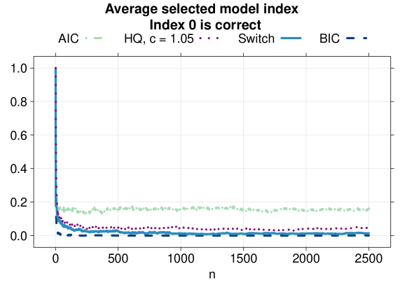
Figure 1: $N=1000$ data sets of length $n=2500$ are generated from a standard normal distribution and the criteria are evaluated at each sample size. The figure shows the average selected model index (0 for $\mathcal{M}_{1}$, 1 for $\mathcal{M}_{2}$). The true index is 0.

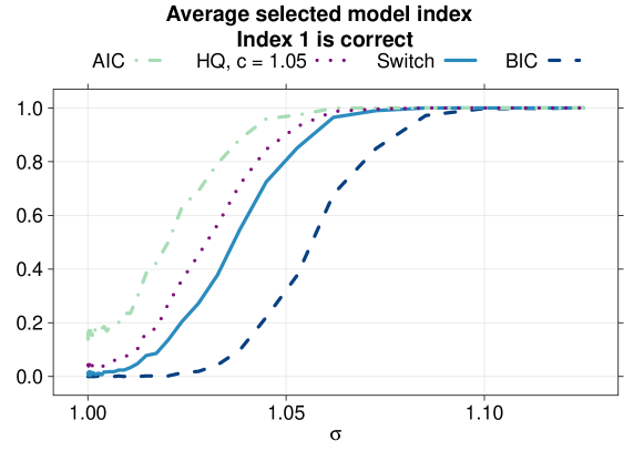
Figure 2: $N=1000$ data sets of length $n=2500$ are generated from a normal distribution with mean 0 and variance $\sigma^{2}$ for a range of values of $\sigma$. The criteria are evaluated at $n=2500$. The figure shows the average selected model index (0 for $\mathcal{M}_{1}$, 1 for $\mathcal{M}_{2}$). The true index is 1.

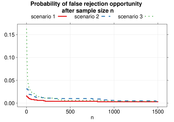
Figure 3: $N=1000$ data sets of length $n_{\text{max}}=10000$ in each scenario, from the simple model. The complex model is selected when $\delta_{\text{sw}}(x^{n})>20$. Estimated probability that there exists a model index after $n$ at which the complex model will be selected. Results shown up to $n=1500$ for clarity. After $n=1500$, the three curves are indistinguishable and all very close to zero.

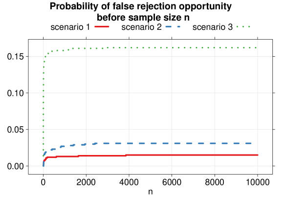
Figure 4: Setting as Figure 3. Estimated probability that there exists a model index before $n$ at which the complex model would have been selected.

6 Discussion and Future Work

In this paper we showed that switching combines near-rate optimality, consistency and, for singleton ${\cal M}_{0}$, robustness to optional stopping. We end the paper by highlighting three issues which, we feel, need additional discussion: first, the desirability of consistency; second, whether there is anything ‘special’ to the switch criterion as opposed to other possible trade-offs between risk optimality and consistency; and third, the limitations of switching in its current form.

Consistency

Since the desirability of consistency, in the sense of finding the smallest model containing the true distribution, is somewhat controversial, let us discuss it a bit further. The main argument against consistency is made by those adhering to Box’s maxim ‘Essentially, all models are wrong, but some are useful’ (Box and Draper, 1987). According to some, the goal of model selection should therefore not be to select a non-existing ‘true’ model, but to obtain the best predictive inference or best inference about a parameter (Burnham and Anderson, 2004; Forster, 2000). Another issue with consistency is that it is a ‘nonuniform’ notion, which in our context means that — as is indeed easy to see — it is impossible to give a bound on the probability under $\mathbb{P}_{\mu}$ of selecting the wrong model at sample size $n$ that converges to $0$ uniformly for all $\mu\in M$. This nonuniformity implies that consistency is of little practical consequence for post-model selection inference (Leeb and Pötscher, 2005).

As to the first argument, one can reply that there do exist situations in which a model can be correct, for example in the field of extrasensory perception (Bem, 2011), in which it seems exceedingly likely that the null model (expressing that no such thing exists) is correct; another example is genetic linkage (Gusella et al., 1983; Tsui et al., 1985). The second argument is more convincing, but only to argue that even if consistency holds, a method may not be very useful in practice. It does not contradict that consistency can sometimes be a highly desirable (but never the only highly desirable) property — we feel that this is the case whenever we are not purely interested in prediction but instead are also seeking to find out whether a certain structural relationship (e.g. dependence between variables) holds or not.

Going one step further, it seems a good idea to study model selection methods not in terms of the asymptotic, nonuniform notion of consistency but instead by a more tangible finite-sample analogue. For the case of just two models, Type-I and Type-II errors provide exactly this analogue — note that if both errors go to 0 as $n\rightarrow\infty$, this implies consistency. Thus, the practical importance of the present work, for us, is mostly that model comparison by switching defines, like Bayes, a robust null hypothesis test — providing Type-I errors irrespective of the stopping rule and thus more in line with actual practice — yet has better Type-II error behaviour, allowing the Type-II error to become small (i.e. the power to go to $1$) whenever the true distribution sits at a distance of order $\sqrt{(\log\log n)/n}$ rather than $\sqrt{(\log n)/n}$, as with Bayes. We only showed robustness for singleton $\mathcal{M}_{0}$, however, and our simulations show that it may fail for composite $\mathcal{M}_{0}$, so the major goal for future work is therefore, to come up with methods that are robust to optional stopping also under composite $\mathcal{M}_{0}$.

How special is the switch distribution?

Since Yang proved that in general, the conflict between consistency and risk-optimality is not resolvable, one might argue that any model selection rule just picks some position in the spectrum of behaviours of consistency vs. risk-optimality. For example, one might have a modified HQ criterion which picks ${\cal M}_{1}$ if, using the same setup and notation as in (5.4),

$$\left|\sum_{i=1}^{n}\tilde{X}_{i}\right|\geq\sqrt{n\log\log\log n}.$$ (6.1)

By the central limit theorem, such a method will be consistent, yet when combined with an efficient estimator will achieve the minimax estimation rate up to a $\log\log\log n$ factor, improving on the switch criterion by an additional logarithm. Note however that both the switch distribution and HQ (with $c>1$) achieve strong consistency. The meaning of strong consistency is illustrated in Figure 3 above: it means that, from some $n$ onward, the wrong model will never be selected any more, no matter how long one keeps sampling. It is easy to see from the law of the iterated logarithm that any strongly consistent method can have rate no faster than order $(\log\log n)/n$ — in particular, (6.1) is not strongly consistent. Thus, in this sense both switching and HQ do take a special place in the consistency vs. risk-optimality spectrum as obtaining the fastest rates compatible with strong consistency, which may be viewed as asymptotic robustness to optional stopping. While this may mostly be of theoretical interest, the switch distribution also takes a special place in terms of its nonasymptotic robustness to optional stopping: again, the law of the iterated logarithm implies that any model comparison method that defines a robust hypothesis test cannot achieve estimation rate better than order $(\log\log n)/n$. Again, the main open question here is whether one can modify it so that robustness for composite ${\cal M}_{0}$ is achieved as well.

Future Work — Limitations of the Switch Distribution and Our Results

Whereas the results in this paper all apply to the original switch distribution as defined by Van Erven et al. (2007) and a simplification thereof, for full robustness to optional stopping with composite ${\cal M}_{0}$, some substantial changes have to be made, as suggested by the results in Figure 4. Initial research suggests that such a modification of the switch distribution might indeed be constructed, based on techniques in Ramdas and Balsubramani (2015); whereas, compared to Bayes factor testing, in the current switch criterion, $p_{B,1}$ is modified to another distribution and $p_{B,0}$ can remain the same, in this new version we would also have to change $p_{B,0}$ — the resulting distribution would not have a Bayesian interpretation any more. While this work is still under development, to avoid the nonrobustness seen in Figure 4 as much as possible, for the time being we recommend using flat priors (but in this case, not completely flat - Jeffreys’ prior on $\mu$ is improper, in which case Theorem 2 holds in none of the scenarios and simulations — not reported here — show that optional stopping robustness is violated).

Another limitation lies not in the switch distribution, but in our results: these are restricted to two nested exponential family models. It would be interesting to extend them to more than two models — highlighting the distinction between model selection and testing — and going beyond exponential families. We are hopeful that switching still behaves well in such contexts — we note that the risk rate convergence results of Van Erven et al. (2012) were for countable, possibly infinite collections of completely general models — but they invariably dealt with the cumulative risk. While all our experiments suggest that small cumulative risk usually goes together with small instantaneous risk, formal analysis of the switch criterion’s instantaneous risk is far more difficult, and the present paper heavily relies on sufficiency to do so — so extension of our results beyond exponential families would be difficult.

Before doing so, we would prefer to modify the switch distribution further, since the present version has a drawback when used in nonsequential settings: the precise results it gives are dependent on the order of the data, even if all the models under consideration are i.i.d. Thus, it would be interesting and challenging to design an alternative, order-independent method that, like the switch distribution, is strongly consistent, near rate- and power-optimal, and is robust to optional stopping under composite $\mathcal{M}_{0}$. Such a method would essentially truly achieve the best of the three worlds we considered in this paper — and this is the method we aim for in our future research.

Appendix A Definitions Concerning and Properties of Exponential Families

The following definitions and properties can all be found in the standard reference (Barndorff-Nielsen, 1978) and, less formally, in (Grünwald, 2007, Chapters 18 and 19).

A $k$-dimensional exponential family is a set of distributions on $\mathcal{X}$, which we invariably represent by the corresponding set of densities $\{p_{\theta}\mid\theta\in\Theta\}$, where $\Theta\subset\mathbb{R}^{k}$, such that any member $p_{\theta}$ can be written as

$$p_{\theta}(x)=\frac{1}{z(\theta)}e^{\theta^{T}\phi(x)}r(x)=e^{\theta^{T}\phi(x)-\psi(\theta)}r(x),$$ (A.1)

where $\phi(x)=(\phi_{1}(x),\ldots,\phi_{k}(x))$ is a sufficient statistic, $r$ is a non-negative function called the carrier, $z$ the partition function and $\psi(\theta)=\log{z(\theta)}$. We assume the representation (A) to be minimal, meaning that the components of $\phi(x)$ are linearly independent.

The parameterization in (A.1) is referred to as the canonical or natural parameterization; we only consider families for which the set $\Theta$ is open and connected. Every exponential family can alternatively be parameterized in terms of its mean-value parameterization, where the family is parameterized by the mean $\mu=\mathbb{E}_{\theta}[\phi(X)]$, with $\mu$ taking values in $M\subset\mathbb{R}$, where $\mu$ as a function of $\theta$ is smooth and strictly increasing; as a consequence, the set $M$ of mean-value parameters corresponding to an open and connected set $\Theta$ is itself also open and connected. Whenever for data $x_{1},\ldots,x_{n}$, we have $\frac{1}{n}\sum_{i=1}^{n}\phi(x_{i})\in M$, then the maximum likelihood is uniquely achieved by the $\mu$ that is itself equal to this value,

$$\widehat{\mu}(x^{n})=\frac{1}{n}\sum_{i=1}^{n}\phi(x_{i}).$$ (A.2)

We thus define the maximum likelihood estimator (MLE) to be equal to (A.2) whenever

$$\frac{1}{n}\sum_{i=1}^{n}\phi(X_{i})\in M.$$ (A.3)

Since the result below which directly involves the MLE (Lemma 3) does not depend on its value for $x^{n}$ with $\frac{1}{n}\sum_{i=1}^{n}\phi(x_{i})\not\in M$, we can leave $\widehat{\mu}(x^{n})$ undefined for such values. However, if we want to use the MLE as a ‘sufficiently efficient’ estimator as used in the statement of Theorem 1, we need to define $\widehat{\mu}(x^{n})$ for such values in such a way that the ‘sufficiently efficient property’ (4.1) is satisfied. The following examples show various ways of constructing such sufficiently efficient estimators.

Example 3.

[Sufficient Efficiency for MLE’s for squared (standardized) error and Hellinger] For many full families such as the full (multivariate) Gaussians, Gamma and many others, (A.3) holds $\mu$-almost surely for each $n$, for all $\mu\in M$. If we compare two families ${\cal M}_{0}$ and ${\cal M}_{1}$ given in their mean-value parameterization with $M_{0}\subset M_{1}$ where ${\cal M}_{1}$ is any such family, then the MLE is almost surely well-defined for $M_{1}$ and thus we need not worry about the issue indicated above. We can then take $\breve{\mu}_{1}:=\widehat{\mu}_{1}$ to be the MLE for $\mathcal{M}_{1}$. To get a sufficiently efficient estimator for $M_{0}$, we take $\breve{\mu}_{0}$ to be the projection of $\widehat{\mu}_{1}$ on the first $m_{0}$ coordinates (usually (A.3) will still hold for $\mathcal{M}_{0}$ and then this $\breve{\mu}_{0}$ will also be the MLE for $\mathcal{M}_{0}$). This pair of estimators will be sufficiently efficient for (standardized) squared error and squared Hellinger distance, i.e. (4.1) holds for these three losses. To show this, note that from Proposition 1, Eq. (A.7), we see that it is sufficient to show that (4.1) holds for the squared error loss. Since the $j$-th component of $\widehat{\mu}_{1}$ is equal to $n^{-1}\sum_{i=1}^{n}\phi_{j}(X_{i})$ and $\mathbb{E}_{\mu_{1}}[n^{-1}\sum_{i=1}^{n}\phi_{j}(X_{i})]=\mu_{1,j}$ and $\text{\sc var}_{\mu_{1}}\left[n^{-1}\sum_{i=1}^{n}\phi_{j}(X_{i})\right]=n^{-1}\text{\sc var}_{\mu_{1}}\left[\phi_{j}(X_{1})\right],$ it suffices to show that

$$\sup_{\mu_{1}\in M^{\prime}_{1}}\sup_{j=1,\ldots,m_{1}}\text{\sc var}_{\mu_{1}}\left[\phi_{j}(X_{1})\right]=O\left(1\right),$$

which is indeed the case since $M^{\prime}_{1}$ is a CINECSI set, so that the variance of all $\phi_{j}$’s is uniformly bounded on $M^{\prime}_{1}$ (Barndorff-Nielsen, 1978).

Example 4.

[Other sufficiently efficient estimators for squared (standardized) error and Hellinger] For models such as the Bernoulli or multinomial, (A.3) may fail to hold with positive probability: the full Bernoulli exponential family does not contain the distributions with $P(X_{1}=1)=1$ and $P(X_{1}=0)=1$, so if after $n$ examples, only zeros or only ones have been observed, the MLE is undefined. We can then go either of three ways. The first way, which we shall not pursue in detail here, is to work with so-called ‘aggregate’ exponential families, which are extensions of full families to their limit points. For models with finite support (such as the multinomial) these are well-defined (Barndorff-Nielsen, 1978, page 154–158) and then the MLE’s for these extended families are almost surely well-defined again, and the MLE’s are sufficiently efficient by the same reasoning as above. Another approach that works in some cases (e.g. multinomial) is to take $\breve{\mu}_{1}$ to be a truncated MLE, that, at sample size $n$, maps $X^{n}$ to the MLE within some CINECSI subset $M^{(n)}_{1}$ of $M_{1}$, where $M_{1}^{(n)}$ converges to $M_{1}$ as $n$ increases in the sense that $\sup_{\mu\in M_{1}^{(n)},\mu^{\prime}\in M_{1}\setminus M_{1}^{(n)}}\|\mu-\mu^{\prime}\|^{2}_{2}=O(1/n)$. The resulting truncated MLE, and its projection on $M_{0}$ (usually itself a truncated MLE) will then again be sufficiently efficient. This approach also works if the models $\mathcal{M}_{0}$ and $\mathcal{M}_{1}$ are not full but restricted families to begin with. For full families though, a more elegant approach than truncating MLE’s is to work with Bayesian posterior MAP estimates with conjugate priors. For steep exponential families (nearly all families one encounters in practice are steep), one can always find conjugate priors such that the Bayes MAP estimates based on these priors exist and take a value in $M_{1}$ almost surely (Grünwald and de Rooij, 2005). They then take the form $\breve{\mu}_{1}=\sum_{i=1}^{n}(\phi(X_{i})+\lambda_{0}\mu^{\circ}_{1})/(n+\lambda_{0})$, where $\lambda_{0}>0$ and $\mu^{\circ}_{1}\in M_{1}$ are determined by the prior. $\breve{\mu}_{0}$ can then again be taken to be the projection of $\breve{\mu}_{1}$ onto $M_{0}$. Under the assumption that $\mu_{1}$ is contained in a CINECSI set $M^{\prime}_{1}$, one can now again show, using the same arguments as in Example 3, that such estimators are sufficiently efficient for squared (standardized) error and Hellinger loss.

Example 5.

[Sufficient Efficiency for Rényi and KL divergence] As is well-known, for the multivariate Gaussian model with fixed covariance matrix, the squared error risk and KL divergence are identical up to constant factors, so the unrestricted MLE’s will still be sufficiently efficient for KL divergence. For other models, though, the MLE will not always be sufficiently efficient. For example, with the Bernoulli model and other models with finite support, to make the unrestricted MLE’s well-defined, we would have to extend the family to its boundary points as indicated in Example 3. Since, however, for any $0<\mu<1$ and $\mu^{\prime}=0$, the KL divergence $D(\mu\|\mu^{\prime})=\infty$ and $\mathbb{P}_{\mu}(\hat{\mu}(X^{n})=\mu^{\prime})>0$, the unrestricted MLE in the full Bernoulli model including the boundaries will have infinite risk and thus will not be sufficiently efficient. The MAP estimators tend to behave better though: Grünwald and de Rooij (2005) implicitly show that for 1-dimensional families, under weak conditions on the family (Condition 1 underneath Theorem 1 in their paper) — which were shown to hold for a number of families such as Bernoulli, Poisson, geometric — sufficient efficiency for the KL divergence still holds for MAP estimators of the form above. We conjecture that a similar result can be shown for multidimensional families, but will not attempt to do so here.

A standard property of exponential families says that, for any $\mu\in M$, any distribution ${\mathbb{Q}}$ on ${\cal X}$ with $\mathbb{E}_{X\sim{\mathbb{Q}}}[\phi(X)]=\mu$, any $\mu^{\prime}\in M$, we have

$$\mathbb{E}_{X\sim{\mathbb{Q}}}\left[\log\frac{p_{\mu}(X)}{p_{\mu^{\prime}}(X)}\right]=\mathbb{E}_{X\sim{\mathbb{P}_{\mu}}}\left[\log\frac{p_{\mu}(X)}{p_{\mu^{\prime}}(X)}\right]=D(\mu\|\mu^{\prime}),$$ (A.4)

the final equality being just the definition of $D(\cdot\|\cdot)$. Now fix an arbitry sample $x^{n}$. By taking ${\mathbb{Q}}$ to be the empirical distribution on ${\cal X}$ corresponding to sample $x^{n}$, it follows from (A.4) that if $\widehat{\mu}(x^{n})\in M$ then also the following relationship holds for any $\mu^{\prime}\in M$:

$$\frac{1}{n}\log{\frac{p_{\widehat{\mu}(x^{n})}(x^{n})}{p_{\mu^{\prime}}(x^{n})}}=D(\widehat{\mu}(x^{n})\|\mu^{\prime}).$$ (A.5)

(A.4) and (A.5) are a direct consequence of the sufficiency of $\widehat{\mu}_{1}(X^{n})$, and folklore among information theorists. For a proof of (A.4) and more details on (A.5), see e.g. (Grünwald, 2007, Chapter 19), who calls this the robustness property of the KL divergence for exponential families.

We are now in a position to prove Proposition 1, which we repeat for convenience.

Proposition 1

Let $M$, a product of open intervals, be the mean-value parameter space of an exponential family, and let $M^{\prime}$ be a CINECSI subset of $M$. Then there exist positive constants $\vec{c}$ such that for all $\mu,\mu^{\prime}\in M^{\prime}$,

$$c_{1}\|\mu^{\prime}-\mu\|^{2}_{2}\leq c_{2}\cdot d_{ST}(\mu^{\prime}\|\mu)\leq d_{H^{2}}(\mu^{\prime},\mu)\leq d_{R}(\mu^{\prime},\mu)\leq D(\mu^{\prime}\|\mu)\leq c_{3}\|\mu^{\prime}-\mu\|^{2}_{2}.$$ (A.6)

and for all $\mu^{\prime}\in M^{\prime},\mu\in M$ (i.e. $\mu$ is now not restricted to lie in $M^{\prime}$),

$$d_{H^{2}}(\mu^{\prime},\mu)\leq c_{4}\|\mu^{\prime}-\mu\|^{2}_{2}\leq c_{5}\cdot d_{ST}(\mu^{\prime}\|\mu)\leq c_{6}\|\mu^{\prime}-\mu\|^{2}_{2}.$$ (A.7)

Proof.

We start with (A.6). The third and fourth inequality are immediate by using $-\log x\geq 1-x$ and Jensen’s inequality, respectively. From standard properties of Fisher information for exponential families (Barndorff-Nielsen, 1978) we have that, for any CINECSI (hence compact and bounded away from the boundaries of $M$) subset $M^{\prime}$ of $M$, there exists positive $\vec{C}$ with

$$0<{C}_{1}=\inf_{\mu\in M^{\prime}}\det I(\mu)<\sup_{\mu\in M^{\prime}}\det I(\mu)=C_{2}<\infty,$$ (A.8)

from which we infer that for all $\mu^{\prime}\in M^{\prime}$, $\mu,\mu^{\prime\prime}\in\mathbb{R}^{m}$,

$$C_{3}\|\mu-\mu^{\prime\prime}\|^{2}_{2}\leq(\mu-\mu^{\prime\prime})^{T}I(\mu^{\prime})(\mu-\mu^{\prime\prime})\leq C_{4}\|\mu-\mu^{\prime\prime}\|^{2}_{2},$$ (A.9)

for some $0<C_{3}\leq C_{4}<\infty$. Using (A.9), the first inequality is immediate, and the final inequality follows straightforwardly from a second-order Taylor approximation of KL divergence as in (Grünwald, 2007, Chapter 4). It only remains to establish the second inequality. Now, since $M^{\prime}$ is CINECSI and hence compact the fifth (rightmost) inequality implies that there is a $C_{5}<\infty$ such that $\sup_{\mu,\mu^{\prime}\in M^{\prime}}D(\mu^{\prime}\|\mu)<C_{5}$ and hence, via the fourth inequality, that $\sup_{\mu,\mu^{\prime}\in M^{\prime}}d_{R}(\mu^{\prime},\mu)<C_{5}$. Equality (3.2) now implies that there is a $C_{6}$ such that

$$\sup_{\mu,\mu^{\prime}\in M^{\prime}}d_{R}(\mu^{\prime},\mu)/d_{H^{2}}(\mu^{\prime},\mu)<C_{6}.$$ (A.10)

Using again (A.8), a second order Taylor approximation as in Van Erven and Harremoës (2014) now gives that for some constant $C_{7}>0$, $\|\mu-\mu^{\prime}\|^{2}_{2}\leq C_{7}d_{R}(\mu^{\prime},\mu)$ for all $\mu,\mu^{\prime}\in M^{\prime}$. The first result, (A.6), now follows upon combining this with (A.10).

As to (A.7), the second and third inequality are immediate from (A.9). For the first inequality, note that, since $M^{\prime}$ is CINECSI and we assume $M$ to be a product of open intervals, there must exist another CINECSI subset $M^{\prime\prime}$ of $M$ strictly containing $M^{\prime}$ such that $\inf_{\mu^{\prime}\in M^{\prime},\mu\in M\setminus M^{\prime\prime}}\|\mu^{\prime}-\mu\|_{2}^{2}=\delta$ for some $\delta>0$. We now distinguish between $\mu$ in (A.7) being an element of (a) $M^{\prime\prime}$ or (b) $M\setminus M^{\prime\prime}$. For case (a) (A.6), with $M^{\prime\prime}$ in the role of $M^{\prime}$, gives that there is a constant $C_{8}$ such that for all $\mu\in M^{\prime\prime}$, $d_{H^{2}}(\mu^{\prime},\mu)\leq C_{8}\|\mu^{\prime}-\mu\|_{2}^{2}$. For case (b), $\mu\in M\setminus M^{\prime\prime}$, we have $\|\mu^{\prime}-\mu\|^{2}_{2}\geq\delta$ and, using that squared Hellinger distance for any pair of distributions is bounded by $2$, we have $d_{H^{2}}(\mu^{\prime},\mu)\leq(2/\delta)\|\mu^{\prime}-\mu\|_{2}^{2}$. Thus, by taking $c_{4}=\max\{C_{8},2/\delta\}$, case (a) and (b) together establish the first inequality in (A.7). ∎

Appendix B Preparation for Proof of Main Result: Results on Large Deviations

Let $\mathcal{M}_{1}$ and $M_{1}$ be as in Theorem 1. For the following result, Lemma 1, we set $\widehat{\mu}^{\prime}_{1}(X^{n}):=n^{-1}\sum\phi(X_{i})$, so that $\widehat{\mu}^{\prime}_{1}(X^{n})=\widehat{\mu}_{1}(X^{n})$ whenever $n^{-1}\sum\phi(X_{i})\in M_{1}$. It is essentially a multidimensional extension of a standard information-theoretic result, with KL divergence replaced by squared error loss. This standard result states the following: whenever ${\cal M}_{1}$ is a single-parameter exponential family (that is, $m_{1}=1$), then for any $\mu\in M_{1}$, all $a,a^{\prime}>0$ with $\mu+a\in M_{1}$, $\mu-a^{\prime}\in M_{1}$,

$$\mathbb{P}_{\mu}(\widehat{\mu}^{\prime}_{1}(X^{n})\geq\mu+a)\leq e^{-nD(\mu+a\|\mu)}.\ \ ;\ \ \mathbb{P}_{\mu}(\widehat{\mu}^{\prime}_{1}(X^{n})\leq\mu-a^{\prime})\leq e^{-nD(\mu-a^{\prime}\|\mu)}.$$ (B.1)

For a simple proof, see (Grünwald, 2007, Section 19.4.2); for discussion see (Csiszár, 1984) — the latter reference gives a multidimensional extension of (B.1) but of a very different kind than Lemma 1 below. To prepare for the lemma, let $\mathcal{M}_{1}$ and $M_{1}$ be as in Theorem 1 and, for any $\mu\in M_{1}$ and any $\vec{a},\vec{b}\in\mathbb{R}^{m_{1}}_{>0}$, define the $\ell_{\infty}$-rectangle $R_{\infty}(\mu,\vec{a},\vec{b})=\{\mu^{\prime}\in\mathbb{R}^{m_{1}}:\forall j=1,\ldots,m_{1},-b_{j}\leq\mu_{j}^{\prime}-\mu_{j}\leq a_{j}\}$.

Lemma 1.

Let $\mathcal{M}_{1}$ and $M_{1}$ be as in Theorem 1 and fix an arbitrary CINECSI subset $M^{\prime}_{1}$ of $M_{1}$. Then there is a $c>0$ (depending on $M^{\prime}_{1}$) such that, for all $\mu\in M_{1}$, all $n$, all $\vec{a},\vec{b}\in\mathbb{R}^{m_{1}}_{>0}$ such that $R_{\infty}(\mu,\vec{a},\vec{b})\subset M^{\prime}_{1}$,

$$\mathbb{P}_{\mu}(\widehat{\mu}^{\prime}_{1}(X^{n})\not\in R_{\infty}(\mu,\vec{a},\vec{b}))\leq 2m_{1}e^{-nc\cdot(\min_{j}\min\{a_{j},b_{j}\})^{2}}.$$ (B.2)

Proof.

For $j=1,\ldots,m_{1}$, $d\in\mathbb{R}$, let $\vec{e_{j}}$ represent the $j$th standard basis vector, such that $\mu+d\vec{e_{j}}=(\mu_{1},\ldots,\mu_{j-1},\mu_{j}+d,\mu_{j+1},\ldots,\mu_{m_{1}})$, and let $D_{\mu+d\vec{e_{j}}}:=D(\mu+d\vec{e_{j}}\|\mu)$. We now have that there exist constants $c_{a,1},\ldots,c_{a,m_{1}},c_{b,1},\ldots,c_{b,m_{1}}>0$ such that for $c:=\min\{c_{a,1},\ldots,c_{a,m_{1}},c_{b,1},\ldots,c_{b,m_{1}}\}$, all $n$,

$$\mathbb{P}_{\mu}(\widehat{\mu}_{1}(X^{n})\not\in R_{\infty}(\mu,\vec{a},\vec{b})) \leq\sum_{j=1}^{m_{1}}\mathbb{P}_{\mu}(\widehat{\mu}_{1,j}(X_{n})\geq\mu_{j}+a_{j})+\sum_{j=1}^{m_{1}}\mathbb{P}_{\mu}(\widehat{\mu}_{1,j}(X^{n})\leq\mu_{j}-b_{j})$$

$$\leq\sum_{j=1}^{m_{1}}\left(e^{-nD_{\mu+a_{j}\vec{e_{j}}}}+e^{-nD_{\mu-b_{j}\vec{e_{j}}}}\right)\leq\sum_{j=1}^{m_{1}}\left(e^{-nc_{a,j}a_{j}^{2}}+e^{-nc_{b,j}b_{j}^{2}}\right)$$

$$\leq 2m_{1}e^{-nc\cdot(\min_{j}\min\{a_{j},b_{j}\})^{2}},$$

Here the first inequality follows from the union bound, and the second follows by applying, for each of the $2m_{1}$ terms, (B.1) above to the one-dimensional exponential sub-family $\{p_{\mu}\mid\mu\in M_{1}\cap\{\mu:\mu=\mu+d\vec{e_{j}}\text{\ for some $d\in{\mathbb{R}}$}\}\}$. The third follows by Proposition 1 together with the equivalence of the $\ell_{2}$ and sup norms on $\mathbb{R}^{m_{1}}$, and the final inequality is immediate. ∎

Lemma 2.

Under conditions and notations as in Theorem 1, let $\mu,\mu^{\prime}$ be elements of $M_{1}$ and suppose $X^{N}=(X_{n_{1}},\ldots,X_{n_{2}})$ is a sequence of i.i.d. observations of length $N$ from $p_{\mu}$. Then, for any $A\in\mathbb{R}$:

$$\mathbb{P}_{\mu}\left(\log{\frac{p_{\mu}(X^{N})}{p_{\mu^{\prime}}(X^{N})}}<A\right)\leq e^{\frac{1}{2}A}e^{-\frac{N}{2}d_{R}(\mu^{\prime},\mu)}.$$ (B.3)

Proof.

For any $A$, by Markov’s inequality:

$$\mathbb{P}_{\mu} \left(\log{\frac{p_{\mu}(X^{N})}{p_{\mu^{\prime}}(X^{N})}}<A\right)=\mathbb{P}_{\mu}\left(\left(\frac{p_{\mu^{\prime}}(X^{N})}{p_{\mu}(X^{N})}\right)^{\frac{1}{2}}>e^{-\frac{1}{2}A}\right)\leq e^{\frac{1}{2}A}\mathbb{E}_{\mu}\left[\left(\frac{p_{\mu^{\prime}}(X^{N})}{p_{\mu}(X^{N})}\right)^{\frac{1}{2}}\right]$$

$$=e^{\frac{1}{2}A}\left(\mathbb{E}_{\mu}\left[\left(\frac{p_{\mu^{\prime}}(X_{n_{1}})}{p_{\mu}(X_{n_{1}})}\right)^{\frac{1}{2}}\right]\right)^{N}=e^{\frac{1}{2}A}e^{\log{\left(\mathbb{E}_{\mu}\left[\left(\frac{p_{\mu^{\prime}}(X_{n_{1}})}{p_{\mu}(X_{n_{1}})}\right)^{\frac{1}{2}}\right]\right)^{N}}}$$

$$=e^{\frac{1}{2}A}e^{-\frac{N}{2}\left(-\frac{1}{1-1/2}\log{\mathbb{E}_{\mu}\left[\left(\frac{p_{\mu^{\prime}}(X_{n_{1}})}{p_{\mu}(X_{n_{1}})}\right)^{\frac{1}{2}}\right]}\right)}=e^{\frac{1}{2}A}e^{-\frac{N}{2}d_{R}(\mu,\mu^{\prime})}.$$ (B.4)

∎

Proposition 2.

Let $\mathcal{M}_{0},\mathcal{M}_{1},M_{0},M_{1}$ be as in Theorem 1 and let $M^{\prime}_{1}$ be a CINECSI subset of $M_{1}$. Then there exists another, larger, CINECSI subset $M^{\prime\prime}_{1}$ of $M_{1}$ and positive constants $\vec{b}$ such that $M^{\prime}_{1}$ is itself a CINECSI subset of $M^{\prime\prime}_{1}$ and for both $j\in\{0,1\}$, the ML estimator $\widehat{\mu}_{j}(x^{n})$ satisfies

$$\sup_{\mu\in M^{\prime}_{1}}P_{\mu}(\widehat{\mu}_{j}(X^{n})\not\in M^{\prime\prime}_{1})\leq\text{\tt small}_{\vec{b}}(n).$$

Proof.

$M_{1}$ can be written as in (3.3), and hence we can define a set

$$M^{\prime\prime}_{1}=[\zeta_{1,1}^{*},\eta_{1,1}^{*}]\times\ldots\times[\zeta_{1,m_{1}}^{*},\eta_{1,m_{1}}^{*}]$$

for values $\zeta_{1,j}^{*},\eta_{1,j}^{*}\in\mathbb{R}$ such that $M^{\prime\prime}_{1}$ is a CINECSI subset of $M_{1}$. Since $M^{\prime}_{1}$ is connected with compact closure in interior of $M_{1}$ and $M^{\prime\prime}_{1}$ is a subset of $M_{1}$, we can choose the $\zeta_{1,j}^{*},\eta_{1,j}^{*}\in\mathbb{R}$ such that $M^{\prime}_{1}$ is itself a CINECSI subset of $M^{\prime\prime}_{1}$. Since $M^{\prime}_{1}$ is connected and its closure is in the interior of $M^{\prime\prime}_{1}$ which is itself compact, it follows that there is some $\delta>0$ such that, for all $\mu^{\prime}_{1}\in M^{\prime}_{1},\mu^{\prime\prime}_{1}\not\in M^{\prime\prime}_{1}$, all $j\in\{1,\ldots,m_{1}\}$, it holds $|\mu^{\prime}_{1,j}-\mu^{\prime\prime}_{1,j}|>\delta$. It now follows from Lemma 1, applied with $\vec{a}$ chosen such that $R_{\infty}(\mu^{\prime},\vec{a})=M^{\prime\prime}_{1}$, that for every $\mu^{\prime}\in M^{\prime}_{1}$, all $n$,

$$\mathbb{P}_{\mu^{\prime}}\left(\widehat{\mu}_{1}(X^{n})\not\in M_{1}^{\prime\prime}\right)\leq C_{1}e^{-nC_{2}\delta^{2}}$$

for some constants $C_{1},C_{2}$. Here we used that by construction, each entry of $\vec{a}$ must be at least as large as $\delta$. Since $\widehat{\mu}_{1,j}(x^{n})$ and $\widehat{\mu}_{0,j}(x^{n})$ coincide for $0<j\leq m_{0}$ and $\widehat{\mu}_{0,j}(x^{n})$ is constant for $m_{0}<j\leq m_{1}$, the result follows for $\widehat{\mu}_{0}(x^{n})$ as well. ∎

Appendix C Preparation for Proof of Main Result: Results on Bayes Factor Model Selection

Lemma 3.

Let $\mathcal{M}_{0},\mathcal{M}_{1},M_{0},M_{1}$ be as in Theorem 1 and let, for $j\in\{0,1\}$, $M^{\prime}_{j}$ be a CINECSI subset of $M_{j}$. For both $j\in\{0,1\}$, there exist positive constants $\vec{c},\vec{b}$ such that for all $\mu_{1}\in M^{\prime}_{1}$,

$$c_{1}\leq{n}^{-m_{j}/2}\cdot\frac{p_{\widehat{\mu}_{j}(X^{n})}(X^{n})}{p_{B,j}(X^{n})}\leq c_{2},$$ (C.1)

with $\mathbb{P}_{\mu_{1}}$-probability at least $1-\text{\tt small}_{\vec{b}}(n)$.

Proof.

For a Bayesian marginal distribution $p_{B}$ defined relative to $m$-dimensional exponential family $\mathcal{M}$ given in its mean-value parameterization $M$, with a prior $\omega(\cdot)$ that is continuous and strictly positive on $M$, we have as a consequence of the familiar Laplace approximation of the Bayesian marginal distribution of exponential famlies as in e.g. (Kass and Raftery, 1995),

$$p_{B}(x^{n})\sim\left(\frac{n}{{2\pi}}\right)^{-m/2}\cdot\frac{\omega(\widehat{\mu}(x^{n}))}{\sqrt{\det I(\widehat{\mu}(x^{n}))}}p_{\widehat{\mu}(x^{n})}(x^{n}).$$

As shown in Theorem 8.1 in (Grünwald, 2007), this statement holds uniformly for all sequences $x^{n}$ with ML estimators in any fixed CINECSI subset $M^{\prime}$ of $M$. By compactness of $M^{\prime}$, and by positive definiteness and continuity of Fisher information for exponential families, the quantity $\omega(\widehat{\mu})/\sqrt{\det I(\widehat{\mu})}$ will be bounded away from zero and infinity on such sequences, and, applying the result to both the families $\mathcal{M}_{0}$ and $\mathcal{M}_{1}$ it follows that there exist $c_{1},c_{2}>0$ such that for all $n$ larger than some $n_{0}$, uniformly for all sequences $x^{n}$ with $\widehat{\mu}_{j}(x^{n})\in M^{\prime}_{j}$, we have:

$$c_{1}\leq{n}^{-m_{j}/2}\cdot\frac{p_{\widehat{\mu}_{j}(x^{n})}(x^{n})}{p_{B,j}(x^{n})}\leq c_{2}.$$ (C.2)

The result now follows by combining this statement with Proposition 2. ∎

Lemma 4.

Let $\mathcal{M}_{0},\mathcal{M}_{1},M_{0}$, $M_{1}$ and the Bayesian marginal distribution $p_{B,0}$ be as in Theorem 1. Let $M^{\prime}_{1}$ be a CINECSI subset of $M_{1}$. Then there exist positive constants $\vec{c}$ and $\vec{b}$ such that for all $n$, all $\mu_{1}\in M^{\prime}_{1}$, all $A\in{\mathbb{R}}$,

$$\mathbb{P}_{\mu_{1}}\left(\log{\frac{p_{B,1}(X^{n})}{p_{B,0}(X^{n})}}<A\right)\leq n^{m_{1}/2}\cdot c_{1}\cdot e^{\frac{1}{2}c_{2}A}e^{-\frac{n}{2}c_{3}\|\mu_{1}-\mu_{0}\|_{2}^{2}}+\text{\tt small}_{\vec{b}}(n),$$

where for each $\mu_{1}$, $\mu_{0}=\Pi_{0}(\mu_{1})$ as in (3.8).

Proof.

Fix constants $C_{1},C_{2}$ such that they are smaller and larger respectively than the constants $c_{1},c_{2}$ from Lemma 3 and define

$$\mathcal{E}_{n}=\left\{X^{n}:C_{1}\leq n^{-m_{1}/2}\frac{p_{\widehat{\mu}_{1}(X^{n})}(X^{n})}{p_{B,1}(X^{n})}\leq C_{2}\right\}.$$

Using Lemma 3, we have that there exists positive $\vec{b}$ such that for all $A\in\mathbb{R}$,

$$\mathbb{P}_{\mu_{1}}\left(\log{\frac{p_{B,1}(X^{n})}{p_{B,0}(X^{n})}}<A\right)$$

$$= \mathbb{P}_{\mu_{1}}\left(\log{\frac{p_{B,1}(X^{n})}{p_{B,0}(X^{n})}}<A,\mathcal{E}_{n}\right)+\mathbb{P}_{\mu_{1}}\left(\log{\frac{p_{B,1}(X^{n})}{p_{B,0}(X^{n})}}<A,{\mathcal{E}}^{c}_{n}\right)$$

$$\leq \mathbb{P}_{\mu_{1}}\left(\log{\frac{C_{2}^{-1}n^{-m_{1}/2}p_{\widehat{\mu}_{1}(X^{n})}(X^{n})}{p_{B,0}(X^{n})}}<A,\mathcal{E}_{n}\right)+\text{\tt small}_{\vec{b}}(n)$$

$$\leq \mathbb{P}_{\mu_{1}}\left(\log{\frac{C_{2}^{-1}n^{-m_{1}/2}p_{{\mu}_{1}}(X^{n})}{p_{B,0}(X^{n})}}<A\right)+\text{\tt small}_{\vec{b}}(n)$$

$$=\mathbb{P}_{\mu_{1}}\left(\log{\frac{p_{{\mu}_{1}}(X^{n})}{p_{B,0}(X^{n})}}<A+\log C_{2}n^{m_{1}/2}\right)+\text{\tt small}_{\vec{b}}(n).$$ (C.3)

To bound this probability further, we need to relate $p_{B,0}$ to $p_{B^{\prime},0}$, the Bayesian marginal likelihood under model $M_{0}$ under a prior with support restricted to a compact set $M^{\prime}_{0}$. To define $M^{\prime}_{0}$, note first that there must exist a CINECSI subset, say $M^{\prime\prime}_{1}$, of $M_{1}$ such that $M^{\prime}_{1}$ is itself a CINECSI subset of $M^{\prime\prime}_{1}$. Take any such $M^{\prime\prime}_{1}$ and let $M^{\prime}_{0}$ be the closure of $M^{\prime\prime}_{1}\cap M_{0}$. Given $\omega$, the prior density on $\Pi^{\prime}(M_{0})$ used in the definition of $p_{B,0}$, define $\omega^{\prime}(\nu)=\omega(\nu)/\int_{\nu\in\Pi^{\prime}(M^{\prime}_{0})}\omega(\nu)d\nu$ as the prior density restricted to and normalized on $\Pi^{\prime}(M^{\prime}_{0})$ and let $p_{B^{\prime},0}$ be the corresponding Bayesian marginal density on $X^{n}$.

To continue bounding (C), define

$$\mathcal{E}^{\prime}_{n}=\left\{X^{n}:C_{3}\leq n^{-m_{0}/2}\frac{p_{\widehat{\mu}_{0}(X^{n})}(X^{n})}{p_{B,0}(X^{n})}\leq C_{4}\text{\ and \ }C_{3}\leq n^{-m_{0}/2}\frac{p_{\widehat{\mu}_{0}(X^{n})}(X^{n})}{p_{B^{\prime},0}(X^{n})}\leq C_{4}\right\},$$

with $C_{3}$ and $C_{4}$ smaller and larger respectively than the constants $c_{1}$ and $c_{2}$ resulting from Lemma 3 (note that Lemma 3 can be applied to $p_{B^{\prime},0}$ as well, by taking $M_{0}$ in that lemma to be the interior of $M^{\prime}_{0}$ as defined here). Set $C_{5}>C_{4}/C_{3}$, and note that for any $A_{1}\in\mathbb{R}$, abbreviating $\mathbb{P}_{\mu_{1}}\left(\log{\frac{p_{\mu_{1}}(X^{n})}{C_{5}p_{B^{\prime},0}(X^{n})}}<A_{1}\right)$ to $p^{*}$, we have

$$\mathbb{P}_{\mu_{1}}\left(\log{\frac{p_{\mu_{1}}(X^{n})}{p_{B,0}(X^{n})}}<A_{1}\right)$$

$$= \mathbb{P}_{\mu_{1}}\left(\log{\frac{p_{\mu_{1}}(X^{n})}{p_{B,0}(X^{n})}}<A_{1},\ \frac{p_{B_{0}}(X^{n})}{p_{B^{\prime},0}(X^{n})}<C_{5}\right)+\mathbb{P}_{\mu_{1}}\left(\log{\frac{p_{\mu_{1}}(X^{n})}{p_{B,0}(X^{n})}}<A_{1},\ \frac{p_{B_{0}}(X^{n})}{p_{B^{\prime},0}(X^{n})}\geq C_{5}\right)$$

$$\leq \mathbb{P}_{\mu_{1}}\left(\log{\frac{p_{\mu_{1}}(X^{n})}{C_{5}p_{B^{\prime},0}(X^{n})}}<A_{1}\right)+\mathbb{P}_{\mu_{1}}\left(p_{B,0}(X^{n})\geq C_{5}p_{B^{\prime},0}(X^{n})\right)$$

$$= p^{*}+\mathbb{P}_{\mu_{1}}\left(p_{B,0}(X^{n})\geq C_{5}p_{B^{\prime},0}(X^{n})\right)$$

$$\leq p^{*}+\mathbb{P}_{\mu_{1}}\left(\frac{p_{B,0}(X^{n})}{p_{B^{\prime},0}(X^{n})}\geq C_{5},\mathcal{E}^{\prime}_{n}\right)+\mathbb{P}_{\mu_{1}}\left(\frac{p_{B,0}(X^{n})}{p_{B^{\prime},0}(X^{n})}\geq C_{5},({\mathcal{E}}^{\prime}_{n})^{c}\right)$$

$$\leq p^{*}+0+\text{\tt small}_{\vec{b}}(n).$$ (C.4)

Now it only remains to bound $p^{*}$. To this end, let

$$C_{6}:=\int_{\nu\in\Pi^{\prime}(M^{\prime}_{0})}\sqrt{\omega(\nu)}d\nu.$$ (C.5)

Since $M^{\prime}_{0}$ has compact closure in the interior of $M_{0}$ and we are assuming that $\omega$ has full support on $M_{0}$, we have that $C_{6}<\infty$.

Now using Markov’s inequality as in the proof of Lemma 2, that is, the first line of (B.4) with $p_{B^{\prime},0}$ in the role of $p_{\mu^{\prime}}$, gives, for any $A_{2}\in\mathbb{R}$,

$$\mathbb{P}_{\mu_{1}}\left(\log\frac{p_{\mu_{1}}(X^{n})}{p_{B^{\prime},0}(X^{n})}<A_{2}\right)\leq e^{\frac{1}{2}{A_{2}}}\mathbb{E}_{\mu_{1}}\left[\left(\frac{p_{B^{\prime},0}(X^{n})}{p_{\mu_{1}}(X^{n})}\right)^{\frac{1}{2}}\right].$$ (C.6)

The expectation on the right can be further bounded, defining $\omega^{\prime\prime}=\sqrt{\omega}/C_{6}$ and noting that $\omega^{\prime\prime}$ is a probability density, as

$$\mathbb{E}_{\mu_{1}}\left[\left(\frac{p_{B^{\prime},0}(X^{n})}{p_{\mu_{1}}(X^{n})}\right)^{\frac{1}{2}}\right] \leq\mathbb{E}_{\mu_{1}}\left[\left(\frac{\int_{\nu\in\Pi^{\prime}(M^{\prime}_{0})}\omega(\nu)^{1/2}p_{\nu}(X^{n})^{1/2}d\nu}{p_{\mu_{1}}(X^{n})^{1/2}}\right)\right]$$

$$=C_{6}\cdot\mathbb{E}_{\mu\sim\omega^{\prime\prime}}\mathbb{E}_{\mu_{1}}\left[\left(\frac{p_{\mu}(X^{n})}{p_{\mu_{1}}(X^{n})}\right)^{\frac{1}{2}}\right]\leq C_{6}\cdot\mathbb{E}_{\mu_{1}}\left[\left(\frac{p_{\mu^{\circ}}(X^{n})}{p_{\mu_{1}}(X^{n})}\right)^{\frac{1}{2}}\right],$$

where $\mu^{\circ}\in M^{\prime}_{0}$ achieves the supremum of $E_{\mu_{1}}\left[\left(\frac{p_{\mu^{\circ}}(X^{n})}{p_{\mu_{1}}(X^{n})}\right)^{\frac{1}{2}}\right]$ within $M^{\prime}_{0}$. By compactness of $M^{\prime}_{0}$ and continuity, this supremum is achieved. The final term can be rewritten, following the same steps as in the second and third line of (B.4), as

$$\mathbb{E}_{\mu_{1}}\left[\left(\frac{p_{\mu^{\circ}}(X^{n})}{p_{\mu_{1}}(X^{n})}\right)^{\frac{1}{2}}\right]=e^{-\frac{n}{2}d_{R}(\mu_{1},\mu^{\circ})}.$$ (C.7)

Since $M^{\prime}_{0}$ and $M^{\prime}_{1}$ are both CINECSI, it now follows from Proposition 1 that for some fixed $C_{7}>0$,

$$d_{R}(\mu_{1},\mu^{\circ})\geq C_{7}\|\mu_{1}-\mu^{\circ}\|^{2}_{2}\geq C_{7}\|\mu_{1}-\mu_{0}\|^{2}_{2},$$ (C.8)

where the latter inequality follows by the definition of $\mu_{0}=\Pi_{0}(\mu_{1})$, see the explanation below (3.8). Combining (C.6), (C.7) and (C.8), we have thus shown that for all $n$, all $\mu_{1}\in M_{1}$, all $A_{2}\in\mathbb{R}$,

$$\mathbb{P}_{\mu_{1}}\left(\log{\frac{p_{\mu_{1}}(X^{n})}{p_{B^{\prime},0}(X^{n})}}<A_{2}\right)\leq C_{6}e^{\frac{1}{2}A^{\prime\prime}}e^{-\frac{n}{2}C_{7}\|\mu_{1}-\mu_{0}\|_{2}^{2}}.$$ (C.9)

The result now follows by combining (C), (C) and (C.9). ∎

Appendix D Proof of Main Result, Theorem 1

Proof Idea

The proof is based on analyzing what happens if $X_{1},X_{2},\ldots,X_{n}$ are sampled from $p_{\mu^{(n)}_{1}}$, where $\mu^{(1)}_{1},\mu^{(2)}_{1},\ldots$ are a sequence of parameters in $M^{\prime}_{1}$. We consider three regimes, depending on how fast (if at all) $\mu_{1}^{(n)}$ converges to $\mu_{0}^{(n)}$ as $n\rightarrow\infty$. Here $\mu_{0}^{(n)}=\Pi_{0}(\mu_{1}^{(n)})$ is the projection of $\mu^{(1)}$ onto $M_{0}$, i.e. the distribution in $M_{0}$ defined, for each $n$, as in (3.8), with $\mu_{1}$ and $\mu_{0}$ in the role of $\mu_{1}^{(n)}$ and $\mu_{0}^{(n)}$, respectively. Our regimes are defined in terms of the function $f$ given by

$$f(n):=\frac{\|\mu_{1}^{(n)}-\mu_{0}^{(n)}\|^{2}_{2}}{\frac{\log\log n}{n}}=\frac{n\cdot\|\mu_{1}^{(n)}-\mu_{0}^{(n)}\|^{2}_{2}}{\log\log n},$$ (D.1)

which indicates how fast $d_{SQ}(\mu_{1}^{(n)},\mu_{0}^{(n)})$ grows relative to the best possible rate $(\log\log n)/n$. We fix appropriate constants $\Gamma_{1}$ and $\Gamma_{2}$, and we distinguish, for all $n$ with $\Gamma_{2}\log n\geq\Gamma_{1}$, the cases:

$$f(n)\in\begin{cases}[0,\Gamma_{1}]&\text{Case 1}\\ [\Gamma_{1},\Gamma_{2}\log n]&\text{Case 2 (Theorem \ref{thm:upperbound})}\\ [\Gamma_{2}\log n,\infty]&\text{Case 3 (Theorem~{}\ref{thm:consistencycomplex})}.\end{cases}$$

For Case 1, the rate is easily seen to be upper bounded by $O((\log\log n)/n)$, as shown inside the proof of Theorem 1. In Case 2, Theorem 4 establishes that the probability that model ${\cal M}_{0}$ is chosen is at most of order $1/(\log n)$, which, as shown inside the proof of Theorem 1, again implies an upper-bound on the rate-of convergence of $O((\log\log n)/n)$. Theorem 3 shows that in Case 3, which includes the case that $\|\mu_{1}^{(n)}-\mu_{0}^{(n)}\|^{2}_{2}$ does not converge at all, the probability that model ${\cal M}_{0}$ is chosen is at most of order $1/n$, which, as again shown inside the proof of Theorem 1, again implies an upper-bound on the rate-of convergence of $O((\log\log n)/n)$.

The two theorems take into account that $\mu_{1}^{(n)}$ is not just a fixed function of $n$, but may in reality be chosen by nature in a worst-case manner, and that $f(n)$ may actually fluctuate between regions for different $n$. Combining these two results, we finally prove the main theorem, Theorem 1.

Theorem 3.

Let $M_{0},M_{1}$, $M^{\prime}_{1}$ and $p_{\text{sw},1}(x^{n})$ be as in Theorem 1. Then there exist positive constants $\vec{b},\vec{c}$ such that for all $\mu_{1}\in M^{\prime}_{1}$, all $n$,

$$\mathbb{P}_{\mu_{1}}\left(\delta_{\text{sw}}(X^{n})=0\right)\leq c_{1}\cdot n^{m_{1}/2}\cdot e^{-c_{2}n\|\mu_{1}^{(n)}-\mu_{0}^{(n)}\|_{2}^{2}}+\text{\tt small}_{\vec{b}}(n),$$ (D.2)

where $\mu_{0}^{(n)}=\Pi_{0}(\mu_{1}^{(n)})$ is as in (3.8). As a consequence, with $\Gamma_{2}:=c_{2}^{-1}(1+m_{1}/2)$, we have the following: for every sequence $\mu_{1}^{(1)},\mu_{1}^{(2)},\ldots$ with $f(n)$ as in (D.1) larger than $\Gamma_{2}\log n$, we have

$$\mathbb{P}_{\mu^{(n)}_{1}}\left(\delta_{\text{sw}}(X^{n})=0\right)\leq\frac{c_{1}}{n}+\text{\tt small}_{\vec{b}}(n).$$

Proof.

We can bound the probability of selecting the simple model by:

$$\mathbb{P}_{\mu_{1}^{(n)}}\left(\delta_{\text{sw}}(X^{n})=0\right) =\mathbb{P}_{\mu_{1}^{(n)}}\left(\frac{{p_{\text{\rm sw},1}}(X^{n})}{p_{B,0}(X^{n})}\leq 1\right)=\mathbb{P}_{\mu_{1}^{(n)}}\left(\frac{\sum_{i=0}^{\infty}\pi(2^{i})\bar{p}_{2^{i}}(X^{n})}{p_{B,0}(X^{n})}\leq 1\right)$$

$$\leq\mathbb{P}_{\mu_{1}^{(n)}}\left(\frac{\pi(1)p_{B,1}(X^{n})}{p_{B,0}(X^{n})}\leq 1\right).$$

Now (D.2) follows directly by applying Lemma 4 to the rightmost probability. For the second part, set $\Gamma_{2}=c_{2}^{-1}(1+m_{1}/2)$. By assumption $f(n)>\Gamma_{2}\log n$, we have $\|\mu_{1}^{(n)}-\mu_{0}^{(n)}\|^{2}_{2}>\Gamma_{2}(\log n)(\log\log n)/n$. Applying (D.2) now gives the desired result.∎

Theorem 4.

Let $f$ be as in (D.1) and $M^{\prime}_{1}$ be as in Theorem 1. For any $\gamma>0$, there exist constants $\Gamma_{1},\Gamma_{3}>0$ such that, for every sequence $\mu_{1}^{(1)},\mu_{1}^{(2)},\ldots$ of elements of $M^{\prime}_{1}$ with for all $n$, $f(n)>\Gamma_{1}$, we have

$$\mathbb{P}_{\mu_{1}^{(n)}}\left(\frac{{p_{\text{\rm sw},1}}(X^{n})}{p_{B,0}(X^{n})}\leq\gamma\right)\leq\frac{\Gamma_{3}}{\log n}.$$ (D.3)

In particular, by taking $\gamma=1$, we have

$${\mathbb{P}}_{\mu^{(n)}_{1}}(\delta_{\text{sw}}(X^{n})=0)\leq\frac{\Gamma_{3}}{\log n}.$$

The probabilities thus converge uniformly at rate $O(1/(\log n))$ for all such sequences $\mu_{1}^{(1)},\mu_{1}^{(2)},\ldots$.

Proof.

We specify $\Gamma_{1}$ later. By assumption, we have $\pi(2^{i})\gtrsim(\log n)^{-\kappa}$ for $i\in\{0,\ldots,\lfloor\log_{2}{n}\rfloor\}$. We can restrict our attention to the strategy that switches to the complex model at the penultimate switching index, due to the following inequality: for any fixed $\gamma$, there exist positive constants $\vec{C}$ such that for all large $n$:

$$\mathbb{P}_{\mu_{1}^{(n)}}\left(\frac{{p_{\text{\rm sw},1}}(X^{n})}{p_{B,0}(X^{n})}\leq\gamma\right) \leq\mathbb{P}_{\mu_{1}^{(n)}}\left(\frac{\sum_{i=0}^{\lfloor\log_{2}{n}\rfloor}\pi(2^{i})\bar{p}_{2^{i}}(X^{n})}{p_{B,0}(X^{n})}\leq\gamma\right)$$

$$\leq\mathbb{P}_{\mu_{1}^{(n)}}\left(\frac{\sum_{i=0}^{\lfloor\log_{2}{n}\rfloor}\bar{p}_{2^{i}}(X^{n})}{p_{B,0}(X^{n})}\leq C_{1}(\log{n})^{\kappa}\right)$$

$$\leq\mathbb{P}_{\mu_{1}^{(n)}}\left(\frac{\bar{p}_{2^{\lfloor\log_{2}{n}\rfloor-1}}(X^{n})}{p_{B,0}(X^{n})}\leq C_{1}(\log{n})^{\kappa}\right)$$

$$=\mathbb{P}_{\mu_{1}^{(n)}}\left(\log{\frac{\bar{p}_{2^{\lfloor\log_{2}{n}\rfloor-1}}(X^{n})}{p_{B,0}(X^{n})}}\leq\kappa\log{\log{n}}+C_{2}\right).$$ (D.4)

For the remainder of this proof, we will denote the penultimate switching index by $n^{*}$, that is: $n^{*}=2^{\lfloor\log_{2}{n}\rfloor-1}$. Now apply Lemma 3 twice, which gives that there exist $C_{3},C_{4}$ such that, with probability at least $1-\text{\tt small}_{\vec{b}}(n)$,

$$\log{\bar{p}_{{n^{*}}}(X^{n})} =\log p_{B,0}(X^{n^{*}})+\log{p_{B,1}(X^{n}|X^{n^{*}})}=$$

$$=\log p_{B,0}(X^{n^{*}})+\log{p_{B,1}(X^{n})}-\log{p_{B,1}(X^{n^{*}})}$$

$$\geq\log p_{B,0}(X^{n^{*}})+\log p_{\widehat{\mu}_{1}(X^{n})}(X^{n})-\log p_{\widehat{\mu}_{1}(X^{n^{*}})}(X^{n^{*}})+\frac{m_{1}}{2}\log{\frac{{n^{*}}}{n}}-C_{3}$$

$$\geq\log p_{B,0}(X^{n^{*}})+\log\frac{p_{\widehat{\mu}_{1}(X^{n})}(X^{n})}{p_{\widehat{\mu}_{1}(X^{n^{*}})}(X^{n^{*}})}-C_{4},$$ (D.5)

where we used that $\log\frac{n^{*}}{n}$ is of the order of a constant, because $n^{*}$ is between $\frac{n}{4}$ and $\frac{n}{2}$. From this, applying again Lemma 3 twice, it follows that there exists $\vec{b}$ and $C_{5},C_{6}$ such that for all $n$, with probability at least $1-\text{\tt small}_{\vec{b}}(n)$,

$$\log\frac{\bar{p}_{{n^{*}}}(X^{n})}{p_{B,0}(X^{n})} \geq\log\frac{p_{B,0}(X^{n^{*}})}{p_{B,0}(X^{n})}+\log\frac{p_{\widehat{\mu}_{1}(X^{n})}(X^{n})}{p_{\widehat{\mu}_{1}(X^{n^{*}})}(X^{n^{*}})}-C_{4}$$

$$=-\log\frac{p_{\widehat{\mu}_{0}(X^{n})}(X^{n})}{p_{\widehat{\mu}_{0}(X^{n^{*}})}(X^{n^{*}})}-\frac{m_{0}}{2}\log{\frac{{n^{*}}}{n}}+\log\frac{p_{\widehat{\mu}_{1}(X^{n})}(X^{n})}{p_{\widehat{\mu}_{1}(X^{n^{*}})}(X^{n^{*}})}-C_{5}$$

$$\geq-\log\frac{p_{\widehat{\mu}_{0}(X^{n})}(X^{n})}{p_{\widehat{\mu}_{0}(X^{n^{*}})}(X^{n^{*}})}+\log\frac{p_{\widehat{\mu}_{1}(X^{n})}(X^{n})}{p_{\widehat{\mu}_{1}(X^{n^{*}})}(X^{n^{*}})}-C_{6}$$ (D.6)

where we again used that $\log\frac{n^{*}}{n}$ can be bounded by constants. Let $\mathcal{B}_{n}$ be the event that (D.6) holds. By (D.4) and (D.6), for all large $n$, all $\beta\geq 1$,

$${\mathbb{P}}_{\mu_{1}^{(n)}}\left(\frac{{p_{\text{\rm sw},1}}(X^{n})}{p_{B,0}(X^{n})}\leq\gamma\right)\leq{\mathbb{P}}_{\mu_{1}^{(n)}}\left(\log{\frac{\bar{p}_{{n^{*}}}(X^{n})}{p_{B,0}(X^{n})}}\leq\kappa\log{\log{n}}+C_{2}\right)$$

$$\leq {\mathbb{P}}_{\mu_{1}^{(n)}}\left(\log{\frac{\bar{p}_{{n^{*}}}(X^{n})}{p_{B,0}(X^{n})}}\leq\kappa\log{\log{n}}+C_{2},\mathcal{B}_{n}\right)+{\mathbb{P}}_{\mu_{1}^{(n)}}\left(\mathcal{B}^{c}_{n}\right)$$

$$\leq {\mathbb{P}}_{\mu_{1}^{(n)}}\left(-\log\frac{p_{\widehat{\mu}_{0}(X^{n})}(X^{n})}{p_{\widehat{\mu}_{0}(X^{n^{*}})}(X^{n^{*}})}+\log\frac{p_{\widehat{\mu}_{1}(X^{n})}(X^{n})}{p_{\widehat{\mu}_{1}(X^{n^{*}})}(X^{n^{*}})}-C_{6}\leq\kappa\log{\log{n}}+C_{2}\right)+\text{\tt small}_{\vec{b}}(n)$$

$$= {\mathbb{P}}_{\mu_{1}^{(n)}}\left(\mathcal{E}^{(1)}_{n}\right)+\text{\tt small}_{\vec{b}}(n)\leq{\mathbb{P}}_{\mu_{1}^{(n)}}\left(\mathcal{E}^{(\beta)}_{n}\right)+\text{\tt small}_{\vec{b}}(n),$$ (D.7)

where we defined

$$\mathcal{E}^{(\beta)}_{n}=\left\{\log\frac{p_{\widehat{\mu}_{1}(X^{n})}(X^{n})}{p_{\widehat{\mu}_{1}(X^{n^{*}})}(X^{n^{*}})}\cdot\frac{p_{\widehat{\mu}_{0}(X^{n^{*}})}(X^{n^{*}})}{p_{\widehat{\mu}_{0}(X^{n})}(X^{n})}\leq A^{(\beta)}_{n}\right\}$$ (D.8)

and, for $\beta\geq 1$, we set $A^{(\beta)}_{n}=\beta\kappa\log\log n+C_{2}-C_{6}$.

Below, if a sample is split up into two parts $x_{1},\ldots,x_{n^{*}}$ and $x_{n^{*}+1},\ldots,x_{n}$, these partial samples will be referred to as $x^{n^{*}}$ and $x^{>n^{*}}$ respectively. We also suppress in our notation the dependency of $A_{n}$, $\mathcal{E}_{n}$ and $\mathcal{D}_{j,n}$ as defined below on $\beta$; all results below hold, with the same constants, for any $\beta\geq 1$.

We will now bound the right-hand side of (D) further. Define the events

$$\mathcal{D}_{1,n} =\left\{\log\frac{p_{\mu_{1}^{(n)}}(x^{n})}{p_{\mu_{1}^{(n)}}(x^{n^{*}})}\leq\log\frac{p_{\widehat{\mu}_{1}(X^{n})}(x^{n})}{p_{\widehat{\mu}_{1}(X^{n^{*}})}(x^{n^{*}})}+A_{n}\right\}$$

$$\mathcal{D}_{0,n} =\left\{\log\frac{p_{\mu_{0}^{(n)}}(x^{n})}{p_{\mu_{0}^{(n)}}(x^{n^{*}})}\geq\log\frac{p_{\widehat{\mu}_{0}(X^{n})}(x^{n})}{p_{\widehat{\mu}_{0}(X^{n^{*}})}(x^{n^{*}})}-A_{n}\right\}.$$

The probability in (D) can be bounded, for all $\beta\geq 1$, as

$${\mathbb{P}}_{\mu_{1}^{(n)}}(\mathcal{E}_{n}) ={\mathbb{P}}_{\mu_{1}^{(n)}}(\mathcal{E}_{n},\mathcal{D}_{0,n}\cap\mathcal{D}_{1,n})+{\mathbb{P}}_{\mu_{1}^{(n)}}(\mathcal{E}_{n},(\mathcal{D}_{0,n}\cap\mathcal{D}_{1,n})^{c})+\text{\tt small}_{\vec{b}}(n)$$

$$\leq{\mathbb{P}}_{\mu_{1}^{(n)}}(\mathcal{E}_{n},\mathcal{D}_{0,n},\mathcal{D}_{1,n})+{\mathbb{P}}_{\mu_{1}^{(n)}}(\mathcal{D}_{1,n}^{c})+{\mathbb{P}}_{\mu_{1}^{(n)}}(\mathcal{D}_{0,n}^{c})+\text{\tt small}_{\vec{b}}(n).$$ (D.9)

We first consider the first probability in (D): there are constants $\vec{C}$ such that, for all large $n$,

$${\mathbb{P}}_{\mu_{1}^{(n)}}(\mathcal{E}_{n},\mathcal{D}_{0,n},\mathcal{D}_{1,n})$$

$$\leq{\mathbb{P}}_{\mu_{1}^{(n)}}\left(\log\frac{p_{{\mu}_{1}^{(n)}}(X^{n})}{p_{\mu_{1}^{(n^{*})}}(X^{n^{*}})}-A_{n}+\log\frac{p_{{\mu}_{0}^{(n)}}(X^{n})}{p_{{\mu}_{0}^{(n)}}(X^{n*})}-A_{n}\leq A_{n}\right)$$

$$={\mathbb{P}}_{\mu_{1}^{(n)}}\left(\log\frac{p_{\mu_{1}^{(n)}}(X^{>n^{*}})}{p_{\mu_{0}^{(n)}}(X^{>n^{*}})}\leq 3A_{n}\right)$$

$$\leq e^{\frac{3}{2}A_{n}}e^{-\frac{n}{4}d_{R}(\mu_{1}^{(n)},\mu_{0}^{(n)})}\leq e^{(3/2)\beta\kappa\log\log n+C_{7}}e^{-C_{8}n\|\mu_{1}^{(n)}-\mu_{0}^{(n)}\|^{2}_{2}}=e^{C_{7}}(\log n)^{(3/2)\beta\kappa-\Gamma_{1}\cdot C_{8}},$$ (D.10)

where $\Gamma_{1}$ is as in the statement of the theorem, the second inequality follows by Lemma 2 and noting $n^{*}<\frac{n}{2}$, we used Proposition 1.

We now consider the second probability in (D). Using $p_{\widehat{\mu}_{1}(X^{n})}(x^{n})\geq p_{\mu_{1}^{(n)}}(x^{n})$ we have the following, where we define the event $\mathcal{F}_{n}=\{\widehat{\mu}_{1}(X^{n^{*}})\in M^{\prime}_{1}\}$ with $M^{\prime}_{1}$ the CINECSI subset of $M_{1}$ mentioned in the theorem statement: there is $C_{9},C_{10}>0$ such that for al large $n$,

$${\mathbb{P}}_{\mu_{1}^{(n)}}(\mathcal{D}_{1,n}^{c}) ={\mathbb{P}}_{\mu_{1}^{(n)}}\left(\log\frac{p_{\mu_{1}^{(n)}}(X^{n})}{p_{\mu_{1}^{(n)}}(X^{n^{*}})}>\log\frac{p_{\widehat{\mu}_{1}(X^{n})}(X^{n})}{p_{\widehat{\mu}_{1}(X^{n^{*}})}(X^{n^{*}})}+A_{n}\right)$$

$$\leq{\mathbb{P}}_{\mu_{1}^{(n)}}\left(\log\frac{p_{\widehat{\mu}_{1}(X^{n})}(X^{n})}{p_{\mu_{1}^{(n)}}(X^{n^{*}})}>\log\frac{p_{\widehat{\mu}_{1}(X^{n})}(X^{n})}{p_{\widehat{\mu}_{1}(X^{n^{*}})}(X^{n^{*}})}+A_{n}\right)$$

$$\leq{\mathbb{P}}_{\mu_{1}^{(n)}}\left(\log\frac{p_{\widehat{\mu}_{1}(X^{n^{*}})}(X^{n^{*}})}{p_{\mu_{1}^{(n)}}(X^{n^{*}})}>A_{n},\mathcal{F}_{n}\right)+{\mathbb{P}}_{\mu_{1}^{(n)}}\left(\mathcal{F}_{n}^{c}\right)$$

$$\leq{\mathbb{P}}_{\mu_{1}^{(n)}}\left(D(\widehat{\mu}_{1}(X^{n^{*}})\|\mu_{1}^{(n)})>A_{n},\mathcal{F}_{n}\right)+\text{\tt small}_{\vec{b}}(n)$$

$$\leq{\mathbb{P}}_{\mu_{1}^{(n)}}\left(\|\widehat{\mu}_{1}(X^{n^{*}})-\mu_{1}^{(n)}\|_{2}^{2}>C_{9}A_{n},\mathcal{F}_{n}\right)+\text{\tt small}_{\vec{b}}(n)$$

$$\leq{\mathbb{P}}_{\mu_{1}^{(n)}}\left(\|\widehat{\mu}_{1}(X^{n^{*}})-\mu_{1}^{(n)}\|_{\infty}>\sqrt{C_{9}A_{n}/m_{1}}\right)+\text{\tt small}_{\vec{b}}(n)$$ (D.11)

$$\leq e^{-C_{10}A_{n}}=e^{-C_{10}(C_{2}-C_{6})}\frac{1}{(\log n)^{C_{10}\beta\kappa}},$$ (D.12)

where we used the KL robustness property (A.5), Proposition 1 and Lemma 1.

The third probability in (D) is considered in a similar way. Using $p_{\widehat{\mu}_{0}(X^{n^{*}})}(X^{n^{*}})\geq p_{\mu_{0}^{(n)}}(X^{n^{*}})$ we have $C_{11},C_{12}>0$ such that:

$${\mathbb{P}}_{\mu_{1}^{(n)}}(\mathcal{D}_{0,n}^{c}) ={\mathbb{P}}_{\mu_{1}^{(n)}}\left(\log\frac{p_{\mu_{0}^{(n)}}(X^{n})}{p_{\mu_{0}^{(n)}}(X^{n^{*}})}<\log\frac{p_{\widehat{\mu}_{0}(X^{n})}(X^{n})}{p_{\widehat{\mu}_{0}(X^{n^{*}})}(X^{n^{*}})}-\frac{1}{3}A_{n}\right)$$

$$\leq{\mathbb{P}}_{\mu_{1}^{(n)}}\left(\log\frac{p_{\mu_{0}^{(n)}}(X^{n})}{p_{\widehat{\mu}_{0}(X^{n^{*}})}(x^{n^{*}})}<\log\frac{p_{\widehat{\mu}_{0}(X^{n})}(X^{n})}{p_{\widehat{\mu}_{0}(X^{n^{*}})}(X^{n^{*}})}-\frac{1}{3}A_{n}\right)$$

$$={\mathbb{P}}_{\mu_{1}^{(n)}}\left(\log\frac{p_{\widehat{\mu}_{0}(X^{n})}(X^{n})}{p_{\mu_{0}^{(n)}}(X^{n})}>\frac{1}{3}A_{n}\right)$$

$$\leq C_{11}\frac{1}{(\log n)^{C_{12}\beta\kappa}}$$ (D.13)

where we omitted the last few steps which are exactly as in (D).

We now finish the proof by combining (D), (D), (D) and (D), which gives that, if we choose $\beta\geq\max\{1/(\kappa C_{10}),1/(\kappa C_{12})\}$ and, for this choice $\beta$, we choose $\Gamma_{1}$ as in (D) as $\Gamma_{1}\geq(1+(3/2)\beta\kappa)/C_{8}$, then we have $\mathbb{P}_{\mu_{1}^{(n)}}(\mathcal{E}_{n})\leq\Gamma_{4}/(\log n)$ for some constant $\Gamma_{4}$ independent of $n$; the result now follows from (D).

∎

Proof of Theorem 1

Proof.

We show the result in two stages. In Stage 1 we provide a tight upper bound on the risk, based on an extension of the decomposition of the risk (3.9) to general families and estimators $\breve{\mu}_{0}$ and $\breve{\mu}_{1}$ that are sufficiently efficient, i.e. that satisfy (4.1), and to losses $d_{\text{\tt gen}}(\cdot\|\cdot)$ equal to squared error loss, standardized squared error loss and KL divergence (it is not sufficient to refer to Proposition 1 and prove the result only for squared error loss, because the equivalence result of Proposition 1 only holds on CINECSI sets and our estimators may take values outside of these; we do not need to consider Rényi and squared Hellinger divergences though, because these are uniformly upper bounded by KL divergence even for $\mu$ outside any CINECSI set). In Stage 2 we show how the bound implies the result.

Stage 1: Decomposition of Upper Bound on the Risk

Let $A_{n}$ be the event that $\mathcal{M}_{1}$ is selected, as in Section 3.3. We will now show that, under the assumptions of Theorem 1, we have for the constant $C$ appearing in (4.1), for all $\mu_{1}\in M^{\prime}_{1}$,

$$R(\mu_{1},\delta,n)\leq\frac{3C}{n}+2\mathbb{P}(A^{c}_{n})d_{\text{\tt gen}}(\mu_{1}\|\mu_{0}),$$ (D.14)

where the left inequality holds for all divergence measures mentioned in the theorem, and the right inequality holds for $d_{\text{\tt gen}}(\cdot\|\cdot)$ set to any of the squared error, the standardized squared error or the KL divergence.

To prove (D.14), we use that for the three divergences of interest, for any $\mu_{1}\in M_{1},\mu\in M_{0}$, with $\mu_{0}\in M_{0}$ as in (3.8), we have

$$d_{\text{\tt gen}}(\mu_{1}\|\mu)\leq 2(d_{\text{\tt gen}}(\mu_{1}\|\mu_{0})+d_{\text{\tt gen}}(\mu_{0}\|\mu)),$$ (D.15)

For $d_{\text{\tt gen}}(\cdot\|\cdot)$ the KL divergence, this follows because

$$D(\mu_{1}\|\mu) =\mathbb{E}_{\mu_{1}}\left[-\log\frac{p_{\mu}(X)}{p_{\mu_{1}}(X)}\right]=\mathbb{E}_{\mu_{1}}\left[-\log\frac{p_{\mu}(X)}{p_{\mu_{0}}(X)}\right]+\mathbb{E}_{\mu_{1}}\left[-\log\frac{p_{\mu_{0}}(X)}{p_{\mu_{1}}(X)}\right]$$

$$=\mathbb{E}_{\mu_{0}}\left[-\log\frac{p_{\mu}(X)}{p_{\mu_{0}}(X)}\right]+\mathbb{E}_{\mu_{1}}\left[-\log\frac{p_{\mu_{0}}(X)}{p_{\mu_{1}}(X)}\right],$$ (D.16)

where the last line follows by the robustness property of exponential families (A.4), since $\mu$ and $\mu_{0}$ are both in $M_{0}$.

For $d_{\text{\tt gen}}(\cdot\|\cdot)$ the squared and standardized squared error case we show (D.15) as follows: Fix a matrix-valued function $J:M_{1}\rightarrow\mathbb{R}^{m_{1}^{2}}$ that maps each $\mu\in M_{1}$ to a positive definite matrix $J_{\mu}$. We can write

$$d_{\text{\tt gen}}(\mu\|\mu^{\prime})=(\mu-\mu^{\prime})^{T}J_{\mu}(\mu-\mu^{\prime}).$$ (D.17)

where $J_{\mu}$ is the identity matrix for the squared error case, and $J_{\mu}$ is the Fisher information matrix for the standardized squared error case. (D.15) follows since we can write, for any function $J_{\mu}$ of the above type including these two:

$$(\mu_{1}-\mu)^{T}J_{\mu_{1}}(\mu_{1}-\mu) =(\mu_{1}-\mu_{0}+\mu_{0}-\mu)^{T}J_{\mu_{1}}(\mu_{1}-\mu_{0}+\mu_{0}-\mu)$$

$$=(\mu_{1}-\mu_{0})^{T}J_{\mu_{1}}(\mu_{1}-\mu_{0})+(\mu_{0}-\mu)^{T}J_{\mu_{1}}(\mu_{0}-\mu)+2(\mu_{1}-\mu_{0})J_{\mu_{1}}(\mu_{0}-\mu)$$

$$\leq 2\left((\mu_{1}-\mu_{0})^{T}J_{\mu_{1}}(\mu_{1}-\mu_{0})+(\mu_{0}-\mu)^{T}J_{\mu_{1}}(\mu_{0}-\mu)\right),$$

where the last line follows because for general positive definite $m\times m$ matrices $J$ and $m$-component column vectors $a$ and $b$, $(b-a)^{T}J(b-a)\geq 0$ so that $b^{T}J(b-a)\geq a^{T}J(b-a)$ and, after rearranging, $b^{T}Jb+a^{T}Ja\geq 2a^{T}Jb$.

We have thus shown (D.15). It now follows that

$$R(\mu_{1},\delta,n) =\mathbb{E}_{\mu_{1}}\left[\textbf{1}_{A_{n}}d_{\text{\tt gen}}(\mu_{1}\|\breve{\mu}_{1}(X^{n}))+\textbf{1}_{A^{c}_{n}}d_{\text{\tt gen}}(\mu_{1}\|\breve{\mu}_{0}(X^{n}))\right]$$

$$\leq\mathbb{E}_{\mu_{1}}\left[d_{\text{\tt gen}}(\mu_{1}\|\breve{\mu}_{1}(X^{n}))+2\cdot\textbf{1}_{A^{c}_{n}}\left(d_{\text{\tt gen}}(\mu_{0}\|\breve{\mu}_{0}(X^{n}))+d_{\text{\tt gen}}(\mu_{1}\|\mu_{0})\right)\right]$$

$$\leq\frac{3C}{n}+2\mathbb{P}(A^{c}_{n})d_{\text{\tt gen}}(\mu_{1}\|\mu_{0}),$$ (D.18)

where we used (D.15) and our condition (4.1) on $\breve{\mu}_{0}$ and $\breve{\mu}_{1}$. We have thus shown (D.14).

Stage 2

We proceed to prove our risk upper bound for the squared error loss, standardized squared error loss and KL divergence, for which the right inequality in (D.14) holds; the result then follows for squared Hellinger and Rényi divergence because these are upper bounded by KL divergence. From (D.14) we see that it is sufficient to show that for all $n$ larger than some $n_{0}$,

$$\sup_{\mu_{1}\in M^{\prime}_{1}}\{\mathbb{P}_{\mu_{1}}(A^{c}_{n})d_{\text{\tt gen}}(\mu_{1}\|\mu_{0})\}=O\left(\frac{\log\log n}{n}\right),$$ (D.19)

for our three choices of $d_{\text{\tt gen}}(\cdot\|\cdot)$. We first note that, since $M^{\prime}_{1}$ is CINECSI, $\sup_{\mu_{1}\in M^{\prime}_{1}}d_{\text{\tt gen}}(\mu_{1}\|\mu_{0})$ is bounded by some constant $C_{1}$. It thus follows by Proposition 2 that there exists some CINECSI subset $M^{\prime\prime}_{1}$ of $M_{1}$ such that, with $B^{c}_{n}\subset A^{c}_{n}$ defined as $B_{n}^{c}=\{x^{n}:\delta(x^{n})=0;\widehat{\mu}_{1}(X^{n})\in M^{\prime\prime}_{1}\}$, we have

$$\sup_{\mu_{1}\in M^{\prime}_{1}}\{\mathbb{P}_{\mu_{1}}(A^{c}_{n})d_{\text{\tt gen}}(\mu_{1}\|\mu_{0})\} =\sup_{\mu_{1}\in M^{\prime}_{1}}\{(\mathbb{P}_{\mu_{1}}(B^{c}_{n})+\mathbb{P}_{\mu_{1}}(A^{c}_{n}\setminus B^{c}_{n}))d_{\text{\tt gen}}(\mu_{1}\|\mu_{0})\}$$

$$=\sup_{\mu_{1}\in M^{\prime}_{1}}\{\mathbb{P}_{\mu_{1}}(B^{c}_{n})d_{\text{\tt gen}}(\mu_{1}\|\mu_{0})\}+C_{1}\cdot\mathbb{P}_{\mu_{1}}(\widehat{\mu}^{(1)}\not\in M^{\prime\prime}_{1})$$

$$=\sup_{\mu_{1}\in M^{\prime}_{1}}\{\mathbb{P}_{\mu_{1}}(B^{c}_{n})d_{\text{\tt gen}}(\mu_{1}\|\mu_{0})\}+\text{\tt small}_{\vec{b}}(n),$$

so that it is sufficient if we can show (D.19) with $B^{c}_{n}$ instead of $A^{c}_{n}$. But on the set $B^{c}_{n}$, all three divergence measures considered are within constant factors of each other, so that it is sufficient if we can show that there is a constant $C_{2}$ such that for all $n$ larger than some $n_{0}$,

$$\sup_{\mu_{1}\in M^{\prime}_{1}}\{\mathbb{P}_{\mu_{1}}(B^{c}_{n})\cdot\|\mu_{1}-\mu_{0}\|^{2}_{2}\}\leq C_{2}\cdot\frac{\log\log n}{n}.$$ (D.20)

Now, fix some $\mu_{1}\equiv\mu_{1}^{(n)}$ and consider $f(n)$ as in (D.1). By Theorem 3, $\mathbb{P}_{\mu_{1}}(B^{c}_{n})\leq C_{3}/n$ for some constant $C_{3}$ that can be chosen uniformly for all $\mu_{1}\in M^{\prime}_{1}$ whenever $f(n)>\Gamma_{2}\log n$ with $\Gamma_{2}$ as in that theorem. Using also that $\|\mu_{1}-\mu_{0}\|^{2}_{2}$ is bounded by $C_{1}$ as above, it follows that (D.20) holds whenever $f(n)>\Gamma_{2}\log n$ and $(C_{1}C_{3})/n\leq C_{2}(\log\log n)/n$, i.e. whenever $f(n)>\Gamma_{2}\log n$ and $C_{2}\geq C_{1}C_{3}/(\log\log n)$.

Second, suppose that $\Gamma_{1}<f(n)\leq\Gamma_{2}\log n$ with $\Gamma_{1}$ as in Theorem 4. Then by that theorem, uniformly for all $\mu^{(n)}_{1}$ with such $f(n)$, we have, with $\Gamma_{3}$ as in that theorem,

$$\|\mu^{(n)}_{1}-\mu^{(n)}_{0}\|^{2}_{2}\cdot{\mathbb{P}}_{\mu^{(n)}_{1}}(\delta_{\text{sw}}(X^{n})=0)=f(n)\cdot\frac{\log\log n}{n}\cdot{\mathbb{P}}_{\mu^{(n)}_{1}}(\delta_{\text{sw}}(X^{n})=0)\leq$$

$$\Gamma_{2}\cdot(\log n)\cdot\frac{\log\log n}{n}\cdot{\mathbb{P}}_{\mu^{(n)}_{1}}(\delta_{\text{sw}}(X^{n})=0)\leq\Gamma_{2}\Gamma_{3}\cdot\frac{\log\log n}{n},$$

where $\mu^{(n)}_{0}=\Pi_{0}(\mu^{(n)}_{1})$ is defined as in (3.8), so that (D.20) holds again whenever $C_{2}\geq\Gamma_{2}\Gamma_{3}$.

Finally, suppose that $f(n)\leq\Gamma_{1}$ with $\Gamma_{1}$ as in Theorem 4. Then (D.20) holds whenever $C_{2}\geq\Gamma_{1}$. Combining the three cases we find that (D.20) holds whenever $C_{3}\geq\max\{\Gamma_{1},\Gamma_{2}\Gamma_{3},\allowbreak C_{1}C_{3}/(\log\log n)\}$; the result is proved.

∎

Appendix E Switching as in Van Erven et al. (2012)

The basic building block of the switch distribution and criterion as formulated by Van Erven et al. (2012) is a countable set of sequential prediction strategies (also known as ‘prequential forecasting systems’ (Dawid, 1984)) $\{p_{k}\mid k\in\mathcal{K}\}$, where $\mathcal{K}$ is a finite or countable set indexing the basic models under consideration. Thus, each model is associated with a corresponding prediction strategy, where a prediction strategy $p$ is a function from $\bigcup_{i\geq 0}\mathcal{X}^{i}$ to the set of densities on $\mathcal{X}$, where $p(\cdot\mid x^{n-1})$ denotes the density on $\mathcal{X}$ that $x^{n-1}$ maps to, and $p(x_{n}\mid x^{n-1})$ is to be interpreted as the probabilistic prediction that strategy $p$ makes for outcome $X_{n}$ upon observation of the first $n-1$ outcomes, $X^{n-1}=x^{n-1}$. For example, for a parametric model $\{p_{\theta}\mid\theta\in\Theta\}$ one can base $p_{k}$ on a Bayesian marginal likelihood, $p_{B}(x^{n}):=\int_{\Theta}\omega(\theta)p_{\theta}(x^{n})d\theta$, where $\omega$ is a prior density on $\Theta$. The corresponding prediction strategy could then be defined by setting $p_{k}(x_{n}\mid x^{n-1}):=p_{B}(x^{n})/p_{B}(x^{n-1})$, the standard Bayesian predictive distribution. In this paper, the basic strategies $p_{k}$ were always Bayesian predictive distributions, but, in the spirit of Dawid (1984), one may consider other choices as well.

After constructing the set of basic prediction strategies, a new family of prediction strategies that switch between the strategies in the set $\{p_{k}\mid k\in\mathcal{K}\}$ is defined. Formally, let $\mathbb{S}$ be the set

$$\mathbb{S}=\left\{\left((t_{1},k_{1}),\ldots,(t_{m},k_{m})\right)\in\left(\mathbb{N}\times\mathcal{K}\right)^{m}|m\in\mathbb{N},1=t_{1}<t_{2}<\ldots<t_{m}\right\}.$$ (E.1)

Each $s\in\mathbb{S}$ specifies the times $t_{1},\ldots,t_{m}$ at which a switch is made between the prediction strategies from the original set, identified by the indices $k_{1},\ldots,k_{m}$. The new family $Q=\{q_{s}\mid s\in\mathbb{S}\}$ is then defined by setting, for all $n,x^{n}\in{\cal X}^{n}$:

$$q_{s}(x_{n}\mid x^{n-1})=p_{k_{j}}(x_{n}\mid x^{n-1}),\quad t_{j}\leq n<t_{j+1},$$ (E.2)

with $t_{m+1}=\infty$ by convention. We now define $q_{s}(x^{n})=\prod_{i=1}^{n}q_{s}(x_{i}\mid x^{i-1})$; one easily verifies that this defines a joint probability density on ${\cal X}^{n}$.

We now place a prior mass function $\pi^{\prime}$ on $\mathbb{S}$ and define, for each $n$, the switch distribution in terms of its joint density for ${\cal X}^{n}$ and $\mathbb{S}$:

$$p_{\text{sw}}(x^{n},s)=q_{s}(x^{n})\pi^{\prime}(s),\quad p_{\text{sw}}(x^{n})=\sum_{s\in\mathbb{S}}p_{\text{sw}}(x^{n},s)=\sum_{s\in\mathbb{S}}q_{s}(x^{n})\pi^{\prime}(s).$$

If the $p_{k}$ are defined as Bayesian predictive distributions as above, then, as explained by Van Erven et al. (2012), the density $p_{\text{sw}}(x^{n})$ can be interpreted as a Bayesian marginal density of $x^{n}$ under the prior $\pi^{\prime}$ on meta-models (model sequences) in $\mathbb{S}$.

The switch distribution can be used to define a model selection criterion $\delta^{\prime}_{\text{sw}}$ by selecting the model with highest posterior probability under the switch distribution. This is done by defining the random variable $K_{n+1}(s)$ on $\mathbb{S}$ to be the index of the prediction strategy that is used by $q_{s}$ to predict the $(n+1)$th outcome. The model selection criterion is then:

$$\delta^{\prime}_{\text{sw}}(x^{n}) =\arg\max_{k}p_{\text{sw}}(K_{n+1}=k\mid x^{n})=\arg\max_{k}\frac{\sum_{s:K_{n+1}(s)=k}p_{\text{sw}}(x^{n},s)}{p_{\text{sw}}(x^{n})}$$

$$=\arg\max_{k}\frac{\sum_{s:K_{n+1}(s)=k}q_{s}(x^{n})\pi^{\prime}(s)}{\sum_{s\in\mathbb{S}}q_{s}(x^{n})\pi^{\prime}(s)},$$ (E.3)

with ties resolved in any way desired.

In our nested two-model case, one might use, for example, a prior $\pi^{\prime}$ with support on

$${\mathbb{S}}^{\prime}=\{(1,0),(1,1),(\;(1,0),(2,1)\;),(\;(1,0),(4,1)\;),(\;(1,0),(8,1)\;),(\;(1,0),(16,1),\ldots\;)\}.$$

Such a prior expresses that at time $1$, for the first prediction, one can either switch to (i.e., start with), model $0$, and keep predicting according to its Bayes predictive distribution — this strategy gets weight $\pi((1,0))$. Or one can start with model $1$, and keep predicting according to its Bayes predictive distribution — this strategy gets weight $\pi((1,1))$. Or one can start with model $0$ and switch to model $1$ after $2^{i}$ observations and then stick with $1$ forever — this strategy gets weight $\pi((\;(1,0),(2^{i},1)\;))$. If we now start with a prior $\pi$ on $\{1,2,\ldots\}$ as in the main text and define $\pi^{\prime}((1,0))=1/2$, $\pi^{\prime}((1,1))=(1/2)\cdot\pi(1)$, and for $i\geq 1$, $\pi^{\prime}((1,0),(2^{i},1))=(1/2)\cdot\pi(2^{i})$, then $\sum_{s\in{\mathbb{S}}^{\prime}}\pi^{\prime}(s)=1$, so $\pi^{\prime}$ is a probability mass function. A simple calculation gives that (E.3) based on switch prior $\pi^{\prime}$ now chooses model $1$ if

$${\sum_{1\leq t<n}\bar{p}_{t}(x^{n})\pi(t)}>{(1+g(n))\cdot p_{B,0}(x^{n})},$$ (E.4)

where $g(n)=\sum_{t\geq n}\pi(t)$; note that $g(n)$ is decreasing and converges to $0$ with increasing $n$. (E.4) is thus an instance of the switch criterion of Van Erven et al. (2012). Comparing this to (2.2), the criterion used in this paper, after rearranging we see that it chooses model $1$ if

$${\sum_{1\leq t<n}\bar{p}_{t}(x^{n})\pi(t)}>(1-g(n))\cdot{p_{B,0}(x^{n})},$$

which is more likely by constant factor to select model $\mathcal{M}_{0}$, the factor however tending to $1$ with increasing $n$. It is completely straightforward to check that Theorem 1 and all other results in this paper still hold if $\delta_{\text{sw}}$ with prior $\pi$ as in the main text is replaced by $\delta^{\prime}_{\text{sw}}$ with corresponding prior $\pi^{\prime}$ as defined here; thus our results carry over to the original definitions of Van Erven et al. (2012). Similarly, the proof for the strong consistency of $\delta^{\prime}_{\text{sw}}$ given by Van Erven et al. (2012) carries through for $\delta_{\text{sw}}$, needing only trivial modifications. From (E.4) we see that modifying the prior $\pi$ in either our or Van Erven et al.’s original criterion has a similar effect as keeping the same $\pi$ but switching between the two versions of the switch criterion.

References

- Akaike (1973) H. Akaike. Information theory and an extension of the maximum likelihood principle. In B. N. Petrov and F. Csaki, editors, Second International Symposium on Information Theory, pages 267–281, Budapest, 1973. Akademiai Kiado.
- Andrews and Baguley (2012) Mark Andrews and Thom Baguley. Prior approval: the growth of Bayesian methods in psychology. British Journal of Mathematical and Statistical Psychology, 66(1):1–7, 2012.
- Barndorff-Nielsen (1978) Ole Barndorff-Nielsen. Information and Exponential Families in Statistical Theory. Wiley, 1978.
- Barron et al. (1998) A. Barron, J. Rissanen, and B. Yu. The minimum description length principle in coding and modeling. IEEE Transactions on Information Theory, 44(6):2743–2760, 1998. Special Commemorative Issue: Information Theory: 1948-1998.
- Barron et al. (1999) Andrew Barron, Lucien Birgé, and Pascal Massart. Risk bounds for model selection via penalization. Probability Theorie and Related Fields, 113(3):301–413, 1999.
- Bem (2011) Daryl J. Bem. Feeling the future: Experimental evidence for anomalous retroactive influences on cognition and affect. Journal of Personality and Social Psychology, 100(3):407–425, 2011.
- Berger and Wolpert (1988) J.O. Berger and R.L. Wolpert. The Likelihood Principle. Institute of Mathematical Statistics, Hayward, CA, 2nd edition, 1988.
- Box and Draper (1987) George E.P. Box and Norman R Draper. Empirical Model-Building and Response Surfaces. Wiley, 1987.
- Burnham and Anderson (2004) K.P. Burnham and D.R. Anderson. Multimodel inference: Understanding AIC and BIC in model selection. Sociological Methods & Research, 33:261–304, 2004.
- Cavanaugh (2012) Joseph E. Cavanaugh. [Catching up faster by switching sooner] : Discussion. Journal of the Royal Statistical Society. Series B (Statistical Methodology), 74(3):402–403, 2012.
- Csiszár (1984) I. Csiszár. Sanov property, generalized -projection and a conditional limit theorem. The Annals of Probability, 12(3):768–793, 1984.
- Dawid (1984) A.P. Dawid. Present position and potential developments: Some personal views, statistical theory, the prequential approach. Journal of the Royal Society, Series A, 147(2):278–292, 1984.
- Dienes (2011) Zoltan Dienes. Bayesian versus orthodox statistics: Which side are you on? Perspectives on Psychological Science, 6(3):274–290, 2011.
- Edwards et al. (1963) Ward Edwards, Harold Lindman, and Leonard J. Savage. Bayesian statistical inference for psychological research. Psychological Review, 70(3):193–242, 1963.
- Efron (1986) Bradley Efron. How biased is the apparent error rate of a prediction rule? Journal of the American Statistical Association, 88(394):461–470, 1986.
- Forster (2000) M.R. Forster. Key concepts in model selection: Performance and generalizability. Journal of Mathematical Psychology, 44:205–231, 2000.
- Grünwald and de Rooij (2005) P. D. Grünwald and S. de Rooij. Asymptotic log-loss of prequential maximum likelihood codes. In Proceedings of the Eighteenth Annual Conference on Computational Learning Theory (COLT 2005), pages 652–667, 2005.
- Grünwald (2007) Peter D. Grünwald. The Minimum Description Length Principle. The MIT Press, 2007.
- Gusella et al. (1983) James. F Gusella, Nancy S. Wexler, P. Michael Conneally, Susan L. Naylor, Mary Anne Anderson, Rudolph E. Tanzi, Paul C. Watkins, Kathleen Ottina, Margaret R. Wallace, Alan Y. Sakaguchi, Anne B. Young, Ira Shoulson, Ernesto Bonilla, and Joseph B. Martin. A polymorphic DNA marker genetically linked to huntington’s disease. Nature, 308:234–238, 1983.
- Hannan and Quinn (1979) Edward J. Hannan and Barry G. Quinn. The determination of the order of an autoregression. Journal of the Royal Statistical Society. Series B (Statistical Methodology), 41(2):190–195, 1979.
- John et al. (2012) Leslie K. John, George Loewenstein, and Drazen Prelec. Measuring the prevalence of questionable research practices with incentives for truth telling. Psychological Science, 23(5):524–532, 2012. 10.1177/0956797611430953.
- Kass and Raftery (1995) R.E. Kass and A. E. Raftery. Bayes factors. Journal of the American Statistical Association, 90(430):773–795, 1995.
- Lauritzen (2012) Steffen Lauritzen. [Catching up faster by switching sooner] : Discussion. Journal of the Royal Statistical Society. Series B (Statistical Methodology), 74(3):401–402, 2012.
- Leeb and Pötscher (2005) Hannes Leeb and Benedikt M. Pötscher. Model selection and inference: Facts and fiction. Econometric Theory, 21(1):21–59, 2005.
- Lhéritier and Cazals (2015) A. Lhéritier and F. Cazals. A sequential nonparametric two-sample test. Technical Report Research Report 8704, INRIA, Sophia Antipolis, 2015.
- Pratt (1962) John W Pratt. On the foundations of statistical inference: Discussion. Journal of the American Statistical Association, pages 307–326, 1962. Discussion.
- Ramdas and Balsubramani (2015) A. Ramdas and A. Balsubramani. Sequential nonparametric testign with the law of the iterated logarithm. Technical Report abs/1506.03488, ArXiv/CoRR, 2015. URL http://arxiv.org/abs/1506.03486.
- Sanborn and Hills (2014) Adam N Sanborn and Thomas T Hills. The frequentist implications of optional stopping on Bayesian hypothesis tests. Psychonomic bulletin & review, 21(2):283–300, 2014.
- Schwarz (1978) G. Schwarz. Estimating the dimension of a model. The Annals of Statistics, 6(2):461–464, 1978.
- Shafer et al. (2011) G. Shafer, A. Shen, N. Vereshchagin, and V. Vovk. Test martingales, Bayes factors and p-values. Statistical Science, 26(1):84–101, 2011.
- Shao (1997) J. Shao. An asymptotic theory for linear model selection. Statistica Sinica, 7:221–264, 1997.
- Stone (1977) M. Stone. An asymptotic equivalence of choice of model by cross-validation and Akaike’s criterion. Journal of the Royal Statistical Society. Series B (Statistical Methodology), 39(1):44–47, 1977.
- Tsui et al. (1985) Lap-Chee Tsui, Manuel Buchwald, David Barker, Jeffrey C. Braman, Robert Knowlton, James W. Schumm, Jan Eiberg, Hans en Mohr, Dara Kennedy, Natasa Plavsic, Martha Zsiga, Danuta Markiewicz, Gita Akots, Valerie Brown, Cynthia Helms, Thomas Gravius, Carol Parker, Kenneth Rediker, and Helen Donis-Keller. Cystic fibrosis locus defined by a genetically linked polymorphic DNA marker. Science, 230:1054–1057, 1985.
- van der Pas (2013) S. L. van der Pas. Almost the best of three worlds. The switch model selection criterion for single-parameter exponential families. Master’s thesis, Leiden University, 2013.
- van der Vaart (1998) Aad W. van der Vaart. Asymptotic Statistics. Cambridge University Press, 1998.
- van Erven and Harremoës (2014) Tim van Erven and Peter Harremoës. Rényi divergence and Kullback-Leibler divergence. IEEE Transactions on Information Theory, 60(7):3797–3820, 2014.
- van Erven et al. (2007) Tim van Erven, P.D. Grünwald, and S. de Rooij. Catching up faster in Bayesian model selection and model averaging. In Advances in Neural Information Processing Systems, volume 20, 2007.
- van Erven et al. (2012) Tim van Erven, Peter D. Grünwald, and Steven De Rooij. Catching up faster by switching sooner: a predictive approach to adaptive estimation with an application to the AIC-BIC dilemma (with discussion). Journal of the Royal Statistical Society. Series B (Statistical Methodology), 74(3):361–417, 2012.
- Wagenmakers (2007) Eric-Jan Wagenmakers. A practical solution to the pervasive problems of -values. Psychonomic Bulletin & Review, 14(5):779–804, 2007.
- Yang (2005) Yuhong Yang. Can the strengths of AIC and BIC be shared? A conflict between model indentification and regression estimation. Biometrika, 92(2):937–950, 2005.