Michel Zamboni-Rached^1,2  and  Erasmo Recami^2,3,4

¹ Photonics Group, Electrical & Computer Engineering, University of Toronto, CA

² DECOM, FEEC, Universidade Estadual de Campinas (UNICAMP), Campinas, SP, Brazil

${}^{3\;}$ Facoltà di Ingegneria, Università statale di Bergamo, Bergamo, Italy.

${}^{4\;}$ INFN—Sezione di Milano, Milan, Italy.

Abstract  –   We propose in detail Antennas for generating Non-Diffracting Beams of Microwaves, for instance with frequencies of the order of 10 GHz, obtaining fair results even when having recourse to realistic apertures endowed with reasonable diameters. Our first proposal refers mainly to sets of suitable annular slits, having in mind various possible applications, including remote sensing.  Our second proposal —which constitutes one of the main aims of this paper— refers to the alternative, rather simple, use of a Parabolic Reflector, illuminated by a spherical wave source located on the paraboloid axis but slightly displaced with respect to the Focus of the Paraboloid. Such a parabolic reflector yields extended focus (non-diffracting) beams. [OCIS codes: 999.9999; 070.7545; 050.1120; 280.0280; 050.1755; 070.0070; 200.0200. Keywords: Non-Diffracting Waves; Microwaves; Remote sensing; Annular Arrays; Bessel beams; Extended focus; Reflecting paraboloids; Parabolic reflectors; Parabolic antennas].

1 Introduction

Since several years it has been discovered that also linear equations like the ordinary wave equations (scalar, vectorial, spinorial…) admit of soliton-like solutions, known as Localized Waves (LW) [1] but that more properly ought to be called Non-diffracting Waves (NDW) [2]. Actually, they possess peculiar properties, as the one of resisting diffraction over long field-depths, and of self-reconstructing themselves after obstacles with size of the order of the antenna’s (and not of their wavelength’s).

They are more suited than the Gaussian waves to represent even elementary particles; and indeed localized solutions exist not only to the K-G or Dirac equations, but also —mutatis mutandis— to the Schroedinger equation (and even to the Einstein equations of GR).

Theory, and applications, of the Non-diffracting Waves have been developed and realized in Acoustics, and even more in Electromagnetism and Optics, during the last two decades, and in particular in recent years. For instance, our first book (J.Wiley, 2008) on NDWs collected the contributions from 10 research groups [its Contents can be downloaded from the site www.unibg.it/recami], while, to our second book (J.Wiley, 2014) on NDWs, 20 research groups contributed.  Indeed, Non-Diffracting Waves are continuously having, and promising, more and more applications. A further interesting fact, a priori, is that their peak-velocities can run from zero to infinity, as it was theoretically derived, in terms of exact analytic solutions, for instance from Maxwell equations only, confirmed by numerical evaluations, and experimentally verified (in the case of optics and microwaves, interesting experimental papers started to appear in the PRL of 1997, while in Acoustics they had started to appear in 1992). But, as we were saying, the NDWs are important for their properties, independently of their peak velocity!  Nevertheless, many people have studied (theoretically, mathematically, and experimentally) the particular NDWs known as “superluminal” X-shaped pulses, it being easier their theoretical and experimental construction. But we later succeeded in studying also the “more orthodox” subluminal solutions, even if expressed in terms of finite-limit integrals, more difficult to be analytically evaluated; and we have in particular discovered how to describe NDWs at rest: i.e., with a static envelope. Such “Frozen Waves” (FW) are expected to have even more incredible applications[3]: e.g., in medicine (for tumor cell destruction, without affecting the front and rear, or surrounding, tissues); or for new types of optical (or acoustic) tweezers; for particle guiding, etc. The FWs have been experimentally produced in Optics in recent times, and in Acoustics (by simulated experiments, this time) even more recently.

To be a little more specific, the NDWs have become a hot topic nowadays in a variety of fields.  In particular, their use, replacing laser beams for achieving multiple traps, has found many potential applications in medicine and biomedicine (see, for instance, Refs.[4, 5, 6, 7, 8]). Even though their simple, multi-ringed structures are not always suitable enough [e.g., they aren’t fit for an effective three-dimensional trap when single beam setups are employed], nevertheless, with today techniques for their generation and real-time control, non-diffracting beams have become —better then focused Gaussian beams or others— indispensable “laser-type” beams for biological studies by means of optical tweezing and micromanipulation techniques. And elsewhere, in fact, the theoretical aspects of an application, for example, in biomedical optics have been presented: Namely, that of Optical Tweezers construction, and of Micro-manipulations, by NDWs in connection with the Generalized Lorenz-Mie Theory[9].

In this paper we propose in detail Antennas for generating Non-Diffracting Beams of Microwaves, for instance with frequencies of the order of 10 GHz, obtaining fair results even when having recourse to realistic apertures possessing reasonable diameters. Our first proposal refers mainly to sets of suitable annular slits, having in mind various possible applications, including remote sensing.  Our second proposal —which constitutes one of the main aims of this paper— refers to the rather simple, alternative use of a Parabolic Reflector, illuminated by a spherical wave source located on the paraboloid axis but slightly displaced with respect to the Focus of the Paraboloid. Such a parabolic reflector yields (non-diffracting) beams with an extended focus.  The present paper reports about work performed by us especially in 2011, and 2012.

1.1 Another brief preamble

Before going on, let us recall —for the readers not well acquainted with the topic— that even finite-energy NDWs (Bessel beams, e.g.), obtained for example by suitable truncations, still keep their extraordinary properties all along their depth of field, much longer that the one possessed by diffracting waves (like the gaussian ones).  Incidentally, the field-depth is as long as the “extended-focus” of the NDW.

Consider for instance a frequency $f$ of 15 GHz, and a finite antenna with radius $R=0.56$ m; and suppose we wish a Bessel beam with initial spot size $r_{0}=9$ cm. We have then to use an axicon angle[1] of 0.055 rad. The field depth, $Z$, of the Bessel beam will be 10.4 m: and the beam will maintain its resolution (spot size and intensity) along all its extended focus (from 0 to 10.4 m). The form of the field intensity in any transverse plane in this range, that is from $z=0$ to about $z=10$ m, is shown in Figure 1.

Figure 1: (Color online) Consider a Bessel beam with initial spot size $r_{0}=9$ cm, frequency $f$ of 15 GHz, and generated by a finite antenna with radius $R=0.56$ m. Its axicon angle[1] is of 0.055 rad, while its field depth will is $Z=10.4$ m (that is, the beam maintains its resolution —spot size and intensity— all along its extended focus). This figure shows the form of its field intensity in any transverse plane in the range from $z=0$ to $z=10.4$ m.

Instead, a gaussian beam with the same initial spot-size, will get the larger spot size of $0.19$ m after 5 m of propagation; and $0.34$ m, even larger, after 10 m of propagation; besides a substantial reduction of the spot intensity.

As a second case, consider a larger aperture radius, $R=1$ m: a Bessel beam with the initial spot-size $r_{0}=17.7$ cm (which correspond to an axicon angle of 0.031 rad) will possess a field depth $Z=33$ m, maintaining its spot size and intensity till the distance of 33 m. The form of the field intensity in any transverse plane in this range, from $z=0$ to $z=33$ m, is shown in Figure 2.

Figure 2: (Color online) As a second case, consider a Bessel beam with initial spot size $r_{0}=17.7$ cm, frequency $f$ of 15 GHz, and generated by a finite antenna with the larger radius $R=1$ m. Its axicon angle[1] is of 0.031 rad, while its field depth will arrive at $Z=10.4$ m (that is, the beam maintains its resolution —spot size and intensity— all along its extended focus). This figure shows the form of its field intensity in any transverse plane in the range from $z=0$ to $z=33$ m.

Instead, after a distance of 33 m, a gaussian beam with the same initial spot-size, will get a quite larger spot-size of $0.62$ m, besides a substantial reduction of its spot intensity.

2 Antennas Generating Non-diffracting Beams
(for remote sensing purposes, et alia)

In our Ref.[10], we already considered the production of truncated pulses, having in mind —among their applications— also remote sensing.

Still for remote sensing et alia, let us here consider further possible antennas, suitable for the generation of non-diffracting beams of microwaves; and choose e.g. the frequency of 15 GHz (and about 1 m for the aperture diameter).  Such an antenna can simply be an array of annular slits[11, 12, 13, 14].  As we were saying, we shall propose later on the alternative use of a parabolic reflector, illuminated by a spherical wave source located on the paraboloid axis but slightly displaced w.r.t. the reflector focus[16, 17].

The said frequency corresponds to a $\lambda$ of 2 cm, and aperture radii much larger than $\lambda$ would be needed for creating highly efficient non-diffracting beams, with spots of the order of $\lambda$ and with a quite large field-depth.

However, we are going to make a more efficient choice from the realistic point of view.

Let us base ourselves on the scalar approximation; and recall that a Bessel beam (Bb) with axial symmetry can be written

$$\psi(\rho,z,t)=J_{0}(k_{\rho}\rho)\exp{i(k_{z}z-\omega t)}\;,$$ (1)

which refers to an ideal beam endowed with an infinite depth of field, that is, with an invariable transverse structure and with a spot given by $\Delta\rho=2.4/k_{\rho}$ at any positions of its. We know that such a Bb would be associated with an infinite power flux through a transverse surface as the $z=0$ one. One needs truncating it by a finite aperture with a radius $R>>\Delta\rho$, and it gets the finite field-depth $Z=R/\tan(\theta)$, where the Bb axicon angle $\theta$ depends on the longitudinal and transverse wavenumbers through the relations $k_{z}=\omega/c\,\cos(\theta)$  and  $k_{\rho}=\omega/c\,\sin(\theta)$.  Simple geometric optics reasonings tell us that, in the region $0<z<Z$ and $0<\rho<(Z-z)\tan(\theta)$, the truncated Bb can still be described by the ideal solution (1).  However, when the aperture radius does not obey the relation $R>>\Delta\rho$, one normally has to resort to lengthy numerical simulations, based on the diffraction integrals, for obtaining the field emanated by the finite antenna. And this is just our case.

However, we have at our disposal the method in Ref.[10] which yields analytic expressions for truncated fields, allowing us to get our results in a few seconds. We already applied it even to antennas composed of annular slits.  Before going on, let us recall also some characteristics of a truncated Bessel beam.  Consider a Bb with axicon angle $\theta=0.062$ rad, and frequency 15 GHz (therefore with spot $\Delta\rho=12$ cm), truncated by a finite circular aperture having radius $R=10$ m.  One expects the emanated field to be approximately given by Eq.(1) in the region $0<z<Z$ and $0<\rho<(Z-z)\tan(\theta)$, with $Z=161.1$ m.  [For the Bb, we are calling spot-radius the distance (in the transverse direction, starting from $\rho=0$) at which one meets the first zero of the field intensity]. The Figures 3 show: the field at the aperture (figure (a)) and its intensity (figure (b)), as well as the 3D intensity of the emanated field (figure (c)) and its projection (figure (d)).

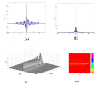
Figure 3: (Color online) Figures referring to a Bb with axicon angle $\theta=0.062$ rad, and frequency 15 GHz (therefore with spot $\Delta\rho=12$ cm), truncated by a finite circular aperture having the large radius $R=10$ m.  One expects the emanated field to be approximately given by Eq.(1) in the region $0<z<Z$ and $0<\rho<(Z-z)\tan(\theta)$, with $Z=161.1$ m.  For comparison, see, by contrast, the case in the next Figure.

If the Bb is truncated by a much smaller aperture (with radius $R=61$ cm) one cannot use any longer for the field-depth the expression $R/\tan(\theta)$ which would yield $Z=9.8$ m.  From the Figures 4 one can see that, on the contrary, the field starts suffering a strong decay at a lower distance, $z\simeq 6$ m; and that the Bb lateral intensity rings (only 3 in this case) start to deteriorate even earlier: Since the intensity rings, too few, are unable to reconstruct the central spot at the (large) distance $Z$.

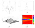
Figure 4: (Color online) Figures showing the behavior of a Bessel beam (Bb) truncated by a finite aperture too small for an efficient non-diffracting beam (see the text): Indeed, only 3 lateral intensity rings survive the truncation.

Nevertheless, even if the Bb starts decaying in this case at $z=6$ m, that is, well before $Z=R/\tan(\theta)=9.8$ m, its spot width keeps its value for larger distances.  Figures 5 depict the Bb transverse intensity at $z=0$ and after $10$ m of propagation: That is, at $z=10$ m. One can see that the spot intensity decays at $1/4$ of its initial value, but its radius changes only a little, from about $\Delta\rho(z=0)=12$ cm  to  $\Delta\rho(z=10\;{\rm m})=15$ cm.

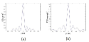
Figure 5: (Color online) Comparison of the transverse shapes of a Bb, truncated by an aperture $R=61$ cm:  (a) in the aperture plane, that is, $z=0$;  and  (b) after $10$ m of propagation, that is, at $z=10$ m.

As we can expect, a gaussian beam with initial spot-radius $\Delta\rho(z=0)=12$ cm would double such a width already at $3.9$ m, while at $z=10$ m its spot would have a central intensity almost 6 times smaller than the initial one and, even worse, a tripled radius ($\Delta\rho(z=10\;{\rm m})=30$ cm).  This is shown by the Figures 6.

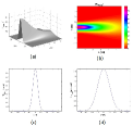
Figure 6: (Color online) Figure showing the evolution of a gaussian beam with the initial spot radius $\Delta\rho=12$ cm.

All what precedes verifies that, even if the last Bessel beam, considered in Figures 4, is so severely truncated as to remain with only 3 of its lateral intensity rings, nevertheless it is still able to keep its spot spatial shape (even if not its intensity) for distances much larger than for a gaussian beam.

Let us go on to our Prototypes (cf. also our second Patent [14]).

2.1 Antennas composed by annular slits

Let us first consider[11, 12, 13, 14] a circular aperture surrounded by a set of concentric annular slits, aiming at producing by such an array (in an approximate way) a Bb with axicon angle $\theta=0.062$ rad, frequency $15$ GHz (with a spot, therefore, $\Delta\rho=12$ cm), truncated by a circular aperture having $R=61$ cm. A simple possibility is modeling the array of annular slits (plus the central aperture), and their excitations, just taking in mind the shape itself of the desired (truncated) Bb: That is to say, we can put the slits between the consecutive zeros of the Bessel function, and illuminate them by uniform fields whose amplitude varies (passing from one slit to the other) according to the maximum magnitude of the Bessel function in the corresponding intervals.

Figure 7 is self-explicative.

Figure 7: (Color online) This figure shows the spatial modeling of our first array of annular slits, and their excitations; on the basis of the desired (truncated) Bb, at $z=0$. The dotted curves refer to the chosen Bessel function, while the steps indicate location and widths of the slits, as well as the uniform field amplitudes to be applied to each of them.

It refers to our first Prototype.  The values of the parameters are:

Prototype no. 1: — $r_{1}=\pi(1+1/4)/k_{\rho}=0.20$ m,  $r_{2}=\pi(2+1/4)/k_{\rho}=0.36$ m,  $r_{3}=\pi(3+1/4)/k_{\rho}=0.52$ m,  $\Delta\rho_{0}=0.23$ m,  $\Delta\rho_{1}=\Delta\rho_{2}=\Delta\rho_{2}=\Delta\rho=0.13$ m,  $\delta_{01}=0.021$ m,  and   $\delta_{12}=\delta_{23}=0.034$ m.   The numerical values of the uniform field amplitudes within each slit are given by the peak values assumed by the Bessel function therein.

Notice that the amplitude values pass from positive to negative values, and viceversa, at each change of slit: This has to be strictly obeyed.  The numerical values of the field in the slits are:  $\Psi_{0}=1$ a.u.,  $\Psi_{1}=J_{0}(k_{\rho}r_{1})=-0.4026$ a.u.,  $\Psi_{2}=J_{0}(k_{\rho}r_{2})=0.3001$ a.u.,  $\Psi_{3}=J_{0}(k_{\rho}r_{3})=-0.2497$ a.u.

Figures 8 show the field emanated by such an antenna.  In figures (a) and (b) the beam does not resemble a truncated Bb, because near the aperture the field is dominated by some isolated intensity peaks (due to the slit edges themselves), which make the field blurred.  However, figures (c) and (d) present the field after $z=2.5$ m, and they do show similarity with a truncated Bb.  In figure (e), the red color (Color online) describes the field at $z=0$; while the dotted line shows the Bessel function “discretized” by the assumed field uniformity inside each slit. Notice that this figure describes the real part of the beam, with its positive or negative values of the amplitude: Such values are to be exactly reproduced in the apparatus for the beam generation.  At last, figure (f) shows the beam transverse intensity shape after 10 m of propagation; that is, at $z=10$ m. Notwithstanding the intensity drop (which decreases to 1/3 of the one at $z=0$), the spot radius varies very little.

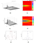
Figure 8: (Color online) Field emanated by Prototype 1.  See the text.

Prototype no. 2: — The spatial structure of the antenna is left unchanged, and one modifies only the value of the uniform fields illuminating the slits. Simply, the uniform field at the circular central aperture is not changed, while inside the slits ($n>1$) the value of each $\Psi_{n}$ is multiplied by $\sqrt{n+1}$.  Therefore:

$\Psi_{0}=1$,  $\Psi_{1}=\sqrt{2}\;J_{0}(k_{\rho}r_{1})=-0.57$ a.u.,  $\Psi_{2}=\sqrt{3}\;J_{0}(k_{\rho}r_{2})=0.52$ a.u.,  $\Psi_{3}=\sqrt{4}\;J_{0}(k_{\rho}r_{3})=-0.5$ a.u.

Figures 9 describe the field emanated by Prototype 2.

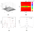
Figure 9: (Color online) Field emanated by Prototype 2.  See the text.

Here the idea is that of increasing the field intensity in the slits (except for the central aperture), since in this way the spot radius does not vary, but the beam intensity distribution at $\rho=0$ gets more homogeneous than for Prototype 1.  One can see, moreover, that the spot intensity at $z=10$ m gets substantially improved.

Prototype no. 3: — Once more, let us keep unaltered the antenna dimensions, and modify only the value of the uniform fields illuminating the slits.  Namely, apply the same amplitude magnitude (that is, the same intensity) to all the slits!, changing only its sign, which will alternately be positive or negative when passing from one slit to the other: In other words, let us change only the phase [by the trivial quantity $\pi$] when going from one slit to the next one.  Numerically, we shall have: $\Psi_{0}=1$ a.u.,  $\Psi_{1}=-1$ a.u.,  $\Psi_{2}=1$ a.u.,  $\Psi_{3}=-1$ a.u.

Figures 10 describe the field emanated by Prototype 3.

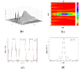
Figure 10: (Color online) Field emanated by Prototype 3.  See the text.

Figure 11: (Color online) The antenna concretely constructed starting from proposals as the above ones[11, 12, 13, 14]; its diameter being 120 cm. More details in Refs.[20, 21]. Photo courtesy of M.Balma.

Notwithstanding the homogeneous intensity distribution in the slits, the emanated field rapidly becomes a beam with a field concentrated around $\rho=0$.  This is just due to the alternate phase change (every time of the quantity $\pi$) when passing from a slit to the next one.

It is worth mentioning that an antenna based on the above proposals[14, 12, 13, 11] has been concretely constructed (see Figure 11) and efficiently applied for obtaining for instance a spot of about 10 cm at a distance of about 10 m, as a significant help for detecting, e.g., buried explosive mines at a safe distance[20, 21, 14].

Let us discuss, and clarify, the structure of the real antenna in Figure 11). It was a product of our approach[11, 12, 13, 14], presented above and exemplified by Figure 7. Within each interval, however, the annular slit was optimized[20, 21] and transformed into a long, spiraling slit. Such spirals were recognized by us to be simply of the Archimede type[15, 14].

In fact, the antenna in Figure 11 (formed by four sets of spirals) does indicate by itself that each one of those sets corresponds to a single Archimede’s spiral: Indeed, by drawing any straight lines passing through the origin, it can be seen that each straight line intersects the spiral at points separated, one from the other, by a constant distance. And this is the fundamental characteristic of an Archimede spiral.

More precisely, the rings constituting the discretized and optimized antenna appear to be formed by slits (we can call them slots), placed along Archimede spirals which go from a root of the Bessel function $J_{0}(k_{\rho}\rho)$ to the next one. If we recall that that an Archimede spiral in polar coordinates gets the simple form  $\rho=a+b\phi$,  with $a$ and $b$ constant, then the previous observation means that we shall have:

$$\rho=\rho_{0i}+b_{i}\phi\ \ \ \rm{for}\ \ \ \rho_{0i}\leq\rho\leq\rho_{i}-\delta/2$$ (2)

where quantities $\rho_{i}$ are the mentioned roots of the Bessel function [given, therefore, by the equation $J_{0}(k_{\rho}\rho_{i})=0$],  it being  $\rho_{01}\equiv\rho_{0}$;   while the subsequent values of $\rho_{0i}$ will obey the relation   $\rho_{0i}=\rho_{i-1}+\delta/2$.  When changing antenna, it will vary only the value of $\delta$.

In general, the values of quantities $b_{i}$ in Eq.(2) are given by

$$b_{i}=\frac{(\rho_{i}-\delta/2)-(\rho_{i-1}+\delta/2)}{2m_{i}\pi}=\frac{\rho_{i}-\rho_{i-1}-\delta}{2m_{i}\pi}$$ (3)

where we called $m_{i}$ the number of turns of the spiral in the interval $\rho_{0i}\leq\rho\leq\rho_{i}-\delta/2$.

The spirals, covering each of the intervals  $\rho_{i}-\delta/2\leq\rho\leq\rho_{i}+\delta/2$, correspond therefore to the quantities

$$\rho=\rho^{\prime}_{0i}+c_{i}\phi$$ (4)

where

$$\rho^{\prime}_{0i}=\rho_{i}-\delta/2$$ (5)

and

$$c_{i}=\frac{(\rho_{i}+\delta/2)-(\rho_{i}-\delta/2)}{2\pi}=\frac{\delta}{2\pi}\ .$$ (6)

If the field is represented by a Bessel-beam field —in which case it can be simply regarded as a linearly polarized field—, then amplitude and phase of each slot can be immediately furnished by the Bessel function.

The antenna in Figure reffigureAntenna constitutes the first concrete example of application of the NDWs in the sector of electromagnetic waves, the unique previous experiment having been the known one by Ranfagni, Mugnai and Ruggeri employing microwaves (but with a demonstrative purpose, and by a totally different technique. A couple of experiments had been also performed in Optics; besides the Lu et al. ones, in Acoustics). Incidentally, our theoretical predictions, and concrete suggestions, were confirmed by the numerical simulations performed in [20] and [21]. One should not forget, moreover, that our antenna using NDWs produces a 10 cm spot till at least 10 m of distance.

Further remarks: (i) the point at which the spirals start, corresponding to the value of $\rho$ that we called $\rho_{0}=\rho_{01}$, is determined a priori, since is given by the shape of the adopted antenna (and it is not at all the origin O);  (ii) the quantity $\delta$ appearing above is nothing but the distance between the rectangles adopted to schematize and discretize (“by steps”) the Bessel function (see Figure 12). We had chosen it as a constant, and it remained so even in the optimized antenna. However, it is chosen a priori; and it might change from a couple of rectangles to the next one, becoming a variable $\delta_{i}rm$;  (iii) one should not forget that each set of slots is a single Archimede spiral (as we specified above).

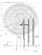
Figure 12: The antenna in the previous figure has been concretely constructed also by exploiting our approach[11, 12, 13, 14], presented in this Section and exemplified by Figure 7. Within each interval, the position of the annular slits was optimized[20, 21], yielding actually spiraling slits: Such spirals were recognized by us to be simply of the Archimede type[14], as explained above.

Some more comments: — We have mentioned above, in particular, the purpose of remote sensing: For instance, of the remote detection of the presence of a buried object. Several approaches may be suggested:

1) In the case of microwaves, one has to produce suitable NDWs. To such an aim, one can suggest their generation:

1a) either by annular slits,

1b) or by a parabolic mirror, with a source slightly displaced from the focal position along the principal axis,

1c) or by circular electric currents; or, rather, by electrically feeding discrete conductive elements, located along rings.

Let us add, however [we are forgetting in this work about the “Frozen Waves”], that one could deal also with:

2) the possibility of producing (by acoustic transducers) a sonic bullet, both for remote detection, and even to the aim of producing by mere compression the explosion of the buried object, in case it is a mine. Let us recall that —in terms of suitable superpositions of equal-frequency Bessel beams— we developed theoretical methods to obtain analytic expression for NDWs even in absorbing media. Anyway, we shall deal in other papers with the (acoustic) case of generators of Non-Diffracting ultrasonic waves.

3 Antenna composed by a Parabolic Reflector and a Spherical Wave Source slightly Displaced w.r.t. the Focus of the Paraboloid

We want now consider just the alternative possibility, based on the properties of the parabolic mirrors, whose equation is  $z=a\rho^{2}$, to use paraboloids as a source of Non-Diffracting microwaves.

It is well known that any ray passing through the focus (at $z_{f}=1/4a$) of a paraboloid is reflected parallel to the reflector axis $z$. If we move our spherical wave source away from the focus (on the $z$-axis and in the positive $z$ direction), the rays striking the reflector will cross the $z$-axis in a position that depends on the incidence point: Namely, the reflected rays will converge on a focal segment (“extended focus”).

Figure 13 is self-explicative. The point $(\rho=0,\ z=z_{f})$ is the paraboloid focus. The point $(\rho=0,\ z=z_{p})$ is situated at the right of the focus. We shall choose a frequency og 30 GHz.

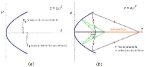
Figure 13: (Color online) Parabolic Reflector with a spherical wave source –assumed to emit, e.g., 30 GHz waves– located along the $z$-axis but at a position shifted with respect to the focus of the Paraboloid: See the text.

Geometric optics tells us that a ray, starting from $z_{p}$ and incident on the paraboloid at the point $(\rho^{\prime},z^{\prime})$, after having been reflected will meet the $z$-axis at a distance $D$ from the reflector vertex given by

$$D=\frac{4az^{\prime 2}+2z^{\prime}+z_{p}}{4az_{p}-1}\;;$$ (7)

this equation yields the minimum and maximum values of $D$ as functions of $z^{\prime}$. Assume that $0\leq z^{\prime}\leq z_{p}$. It is easy to show[16, 17] that

$$D_{{\rm min}}\;=\;\frac{z_{p}}{4az_{p}-1}\;,$$ (8)

while the $D_{{\rm max}}$ corresponding to $z^{\prime}=z_{p}$ is

$$D_{{\rm max}}\;=\;\frac{4az_{p}^{2}+3z_{p}}{4az_{p}-1}\;=\;z_{p}+4D_{{\rm min}}\;.$$ (9)

One therefore gets that the “focal width” $Z_{\rm focalwidth}$ will be

$$Z_{\rm focalwidth}\;=\;D_{{\rm max}}-D_{{\rm min}}\;=\;z_{p}+3D_{{\rm min}}=z_{p}+\frac{3z_{p}}{4az_{p}-1}\;.$$ (10)

In many situations one has $z_{p}<<D_{{\rm min}}$, so that:[16, 17]

$$Z_{\rm focalwidth}\approx\frac{3z_{p}}{4az_{p}-1}\;=\;3D_{{\rm min}}\;.$$ (11)

A basic characteristic of ND beams is possessing not a point-like focus, but just an extended focus (or focal segment): Therefore, one can intuitively expect the present setup to furnish a beam of non-diffracting (ND) type; even if all these considerations are based on geometric optics, which implies for instance (as a necessary, but not sufficient, condition) that the paraboloid size is much bigger than $\lambda$. If we suppose the emanated field to be non-diffracting, this will take place in the interval $D_{{\rm min}}<z<D_{{\rm max}}$.  When it is, moreover, $z_{p}<<D_{{\rm min}}$, that interval becomes  $D_{{\rm min}}<z<4D_{{\rm min}}$,  with  $D_{{\rm min}}=z_{p}/(4az_{p}-1)$:  And our “ND beam” will start to exist at the distance $D_{{\rm min}}$ from the antenna, and will go on existing till the triple of such a distance.

Before going on, let us repeat that the present paper reports about work performed by us during 2011, and 2012.  Subsequently, however, further analogous work on the use of paraboloids as antennas has been done by other friends of ours: So that the interested reader might find more results in Refs.[18, 19].

When a ND beam is generated in the interval $D_{{\rm min}}<z<3D_{{\rm min}}$, the interesting problem arises of knowing the evolution of its transverse intensity during propagation[16, 17, 18, 19]. Some information can be obtained on the basis of the following considerations, which imply however that the parabolic reflector be much, much larger than $\lambda$ (a situation certainly true in Optics, but not necessarily for microwaves).  Let us imagine of dividing the reflector into circular rings (see cintur o, in Figure 14) of sufficiently small width; and afterward of splitting each ring into flat elements, sufficiently small as well but with sizes much larger than $\lambda$.  One can then think that each portion of the spherical wave (originated at $\rho=0,z=z_{p}$), when incident on one of such flat elements, is reflected in the form of a portion of planewave (having the size of the considered flat element) and travels without appreciable diffraction till the $z$-axis. Thus, at each point of the $z$-axis it will arrive a set of small portions of plane waves reflected by the corresponding circular ring.. For symmetry reasons, the wave-vectors of the said set of small portions of planewave will stay on the surface of a cone with angle $2\theta$. See Figure 14. Such a superposition will give rise to a Bessel beam with axicon angle $\theta$, that will propagate along a short interval of $z$, being then replaced by the Bessel beam coming from the next circular ring. This will repeat itself till the distance $D_{{\rm max}}$.

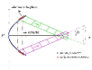
Figure 14: (Color online) Discretization of the paraboloid into circular rings (see cintur o, in the Figure) , with a successive discretization of the rings themselves into flat elements. The figure also shows the portions of wave reflected by two of such flat elements. See the text.

Still from purely geometric considerations, is follows also that:[16, 17]

$$\sin\theta\;=\;\frac{1}{\sqrt{\left(\frac{z-a\eta^{2}}{\eta}\right)^{2}+1}}$$ (12)

where

$$\eta\;=\;\sqrt{-\frac{1}{4a^{2}}+\frac{1}{4a^{2}}\sqrt{1-4a(z_{p}-(4az_{p}-1)z)}}\ .$$ (13)

This allows us to state, even if in an approximate way, that all along the “extended focus”, and for point near the $z$-axis, the field will be proportional to a Bessel function with a (variable) axicon angle $\theta$. That is:

$$\Psi(\rho,z,t)\propto e^{-i\omega t}J_{0}\left(\frac{\omega}{c}\sin\theta\,\rho\right)\;$$ (14)

where $\theta$ is a complicate function of $z$, as we have just seen above; and we still choose a 30 GHz frequency.  In the last equation, the proportionality symbol means “except for a multiplicative function depending on $z$ and $\rho$:”  It is this function that determines the magnitude of the wave. Therefore, the approximate expression (14) does not yield the varying intensity of the field during propagation, but only its transverse behavior.

— Let us now propose the following antenna:

• Position of the focus: $z=z_{f}=0.5\,$m  (so that $a=1/4z_{f}=0.5\,m^{-1}$);

• Position of the spherical wave (30 GHz) source: $z=z_{p}=0.525\,$m  (shifted 2.5 cm from the focus in the positive $z$ direction).

Assuming for the paraboloid $0\leq z\leq z_{p}$, its “mouth” will have a radius $R=1.02\,$m.  Such a configuration furnishes: $D_{{\rm min}}=11.02\,$m    $D_{{\rm max}}=42.52\,$m;  and one does expect that along the segment $D_{{\rm min}}<z<D_{{\rm max}}$ a ND beam is formed. Figure 15 shows intensity and evolution of its transverse shape, according to Eq.(14). [Let us repeat that such a Figure gives us information on the evolution, starting from the the aperture, of the transverse behavior, but not yet the exact intensity of the produced beam].

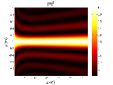
Figure 15: (Color online) Orthogonal, transverse projection of the field emanated by the parabolic reflector, when assuming: Position of the focus, $z=z_{f}=0.5\,$m  (so that $a=1/4z_{f}=0.5\,m^{-1}$);  Position of the spherical wave (30 GHz) source: $z=z_{p}=0.525\,$m  (shifted 2.5 cm from the focus in the positive $z$ direction). See the text. This Figure shows intensity and evolution of the emanated field, according to Eq.(14). [Let us recall that this Figure gives us information on the evolution, starting from the the aperture, of the field transverse behavior, but not the exact intensity of the produced beam].

One can see that this beam possesses an initial spot with radius $\Delta\rho(z=0)=50\,$cm, if we choose as spot radius the value of $\rho$ where it occurs the first zero of the field intensity. Subsequently, the spot radius changes during propagation, diminishing till the approximate value of 24 cm at the point $z\approx 18\,$m, beyond which it starts to increase again, ending with a value of about 31 cm at $z=45\,$m. Roughly speaking, we can call such a beam a “ND beam”, since its spot radius does not exceed the initial value even after having traveled for long distances.

Figure 16 shows the variation of the spot radius as a function of the distance from the aperture. It represents a ND beam generated along more than 30 m; but such a value should not be taken literally since we adopted a model developed “in Optics”, that is, when the reflectors can easily have sizes much bigger than $\lambda$.

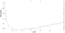
Figure 16: (Color online) Variation of the spot radius for the produced beam, as a function of the distance from the aperture. See the text.

— Some further examples and results:

Let us mention some further results. Assume again, for the paraboloid, the focal position at 0.5 m, and a radius at its mouth of 1 m. We can locate a source of the spherical waves, with frequency 30 GHz, by shifting it a little bit w.r.t. the reflector focus, in order that the initial spot of the generated field is of about 10 cm.  Figure 17 shows that such a spot, even with a non constant intensity, goes on keeping its size —apart from a slight enlargement— till a distance of almost 50 m. The underlying analysis has still been scalar.  The following two Figures show, for comparison, the behavior of analogous gaussian beams: They, when starting with the same spot size, get a field-depth of less than 6 m.

Figure 17: (Color online) Orthogonal, transverse projection of the field emanated by an identical parabolic reflector, when the source of spherical waves (with frequency 30 GHz) is slightly displaced w.r.t. the focus, so that the initial spot of the generated field is of about 10 cm. One can see that such a spot, even with a non constant intensity, goes on keeping its size —apart from a slight enlargement— till a distance of almost 50 m  (the underlying analysis has still been scalar).  The following two Figures show, for comparison, the behavior of analogous gaussian beams.

Figure 18: (Color online) For comparison with the previous Figure, notice as a gaussian beam with the same initial spot possesses a depth of field of less than 6 m.  The present Figure refers to a gaussian beam with focal point at $z=0$.

Figure 19: (Color online) The same as in the previous Figure, when the gaussian beam focal point is located at $z=22$ m.  Again, the field depth is of less than 6 m, instead of almost 50 m.

— A few final considerations:

Various other antennas are possible, varying the values of $z_{f}$ and $z_{p}$; besides modifying the antenna size itself.

But let us spend, rather, a few words about the spherical wave source (cf. Figure 20a) to be located at $z=z_{p}$. Of course, it cannot be large, to avoid blocking a considerable part of the wave reflected by the paraboloid. We may just set forth one suggestion: One can think to open a circular hole around the paraboloid vertex, and send through it a collimated beam parallel to the $z$-axis. At position $z_{p}$ we can then put a spherical reflector (see Figure 20b), so that the parallel rays (coming from the hole created around the paraboloid vertex) are reflected towards the interior of the paraboloid itself. These rays would behave as if emitted from the point $z_{p}$.

Of course, the hole radius must be smaller than or equal to the reflecting spherical mirror’s, both radii having to be as small as possible; at last, the beam entering the hole must remain parallel to $z$ as much as possible.  A problem which remains to be taken into account is that the intensity of the rays reflected by the spherical mirror is not isotropic, lowering its value for increasing reflection angle.

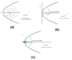
Figure 20: (Color online) The source of spherical waves, located at $z=z_{p}$, can be approximated by a spherical, or hyperbolic, mirror (sub-reflector) reflecting the radiation coming from a suitable hole surrounding the vertex.  See the text for more details.

4 Acknowledgements

The present work has been partially supported by FAPESP, CAPES and CNPq (Brazil), and by INFN (Italy). For kind collaboration or useful discussions during the past several years, the authors are grateful to I.A.Besieris, R.Bonifacio, C.Castro, R.Chiao, C.Conti, A.Friberg, D.Faccio, F.Fontana, E.Giannetto, P.Hawkes, R.Grunwald, G.Maccarini, M.Mattiuzzi, C.Meroni, P.Milonni, M.Novello, S.Paleari, C.Papa, P.Riva, J.L.Prego-Borges, P.Saari, A.Santambrogio, A.Shaarawi, M.Tygel, A.Utkin, R.Ziolkowski, and particularly to M.Balma, D.Campbell, H.E.Hernández-Figueroa, and M.Mojahedi.

References

- [1] Localized Waves, ed. by H.E.Hernández-Figueroa, M.Zamboni-Rached, and E.Recami; book of 386 pages (J.Wiley; New York, 2008): ISBN 978-0470-10885-7.
- [2] Non-Diffracting Waves, ed. by H.E.Hernández-Figueroa, E.Recami, and M.Zamboni-Rached; book of 512 pages (J.Wiley-VCH; Berlin, 2014): ISBN 978-3-527-41195-5.
- [3] E.Recami, M.Zamboni-Rached, H.E.Hernández-Figueroa, et al., “Method and Apparatus for Producing Stationary Intense Wavefields of arbitrary shape”, Patent no. US-2011/0100880 [granted], pub. date 05/05/11: the sponsor being “Bracco Imaging, Spa” [available, e.g., at http://www.google.com.br/url?url=http://patentimages.storage.googleapis.com/pdfs /US20110100880.pdf&rct=j&frm=1&q=&esrc=s&sa=U&ei=Xrv2U5KPHOvesAT5y 5y4DABg&ved=0CCAQFjAD&usg=AFQjCNHZ4xV-pa05-M6yqMtDFaGALQdKGQ ]
- [4] J.Arlt, V.Garcés-Chavez, W.Sibbett and K.Dholakia: “Optical micromanipulation using a Bessel light beam”, Optics Communications 197 (2001) 239-245.
- [5] R.M.Herman and T.A.Wiggins: “Production and uses of diffractionless beams”, Journal of the Optical Society of America A8 (1991) 932-942.
- [6] V.Garcés-Chavez, D.McGloin, H.Melville, W.Sibbett and K.Dholakia: “Simultaneous micromanipulation in multiple planes using a self-reconstructing light beam”, Nature 419 (2002) 145-147.
- [7] V.Garcś-Chávez, D.Roskey, M.D.Summers, H.Melville, D.McGloin, E.M.Wright and K.Dholakia: “Optical levitation in a Bessel light beam”, Appl. Phys. Lett. 85 (2004) 4001-4003.
- [8] G.Milne, K.Dholakia, D.McGloin, K.Volke-Sepulveda and P. Zemánek: “Transverse particle dynamics in a Bessel beam”, Opt. Express 15 (2007) 13972-13987.
- [9] E.Recami, M.Zamboni-Rached, H.E.Hernández-Figueroa, and L.A.Ambrosio, “Non-Diffracting Waves: An introduction”, Chap.1 in the book [2]; and refs. therein.
- [10] M.Zamboni-Rached, E.Recami and M.Balma: “Simple and effective method for the analytic description of important optical beams when truncated by finite apertures”, Applied Optics 51 (2012) 3370-3379 [DOI 1559-128X/12/163370-10].
- [11] M.Zamboni-Rached and E.Recami, “Antenne (annular arrays) generatrici di fasci non-diffrattivi per remote sensing”, Report of January 20, 2011, to M.Balma (unpublished).
- [12] M.Zamboni-Rached, E.Recami, and M.Balma: “Proposte di Antenne generatrici di Fasci Non-diffrattivi per Micro-onde”, e-print posted as arXiv:1108.2027[physics.gen-ph]; August 09, 2011.
- [13] M.Zamboni-Rached, E.Recami, and M.Balma: “Analytic descriptions of optical beams truncated by finite apertures”, in Progress in Electromagnetics Research Symposium (PIERS) Proceedings, Moscow, Russia, Aug. 2012; pp.464-468 [ISSN 1559-9450].
- [14] M.Balma, G.Guarnieri, G.Mauriello, E.Recami and M.Zamboni-Rached (inventors), “Slotted Waveguide Antenna for Near Field Focalization of an Electromagnetic Radiation”, Applicant Selex ES SpA, Patent WO/2013098795/AI with International Application no. PCT/IB2012/057802 of Dec.28, 2012 [available at http://www.google.com/patents/WO2013098795A1?cl=en ]
- [15] M.Zamboni-Rached and E.Recami, “ ‘Interpolazione’ degli slots che appaiono nelle antenne discretizzate e ottimizzaqte”, Report of November 05, 2011, to M.Balma (unpublished).
- [16] M.Zamboni-Rached and E.Recami, “Paraboloidi quali antenne generatrici di fasci non-diffrattivi”, Report of March 23, 2011, to M.Balma (unpublished).
- [17] See, e.g., M.Zamboni-Rached and E.Recami, “Refletores parabólicos Geradores de Feixes Nao-Difrativos”, Report July 25, 2012, to M.Balma (unpublished).
- [18] M.C.de Assis, “Refletores parabolicos usados na geracao de feixes nao-difrativos”, M.Zamboni-Rached supervisor. MSc thesis: D.M.O., FEEC, UNICAMP (Campinas, SP, Brazil), 15/02/2013.
- [19] M.C.de Assis, M.Zamboni-Rached, and L.Ambrósio: (in preparation, 2014)
- [20] D.Devona, A.Delogu, W.Ferrarese, G.Guarnieri, and G.Mauriello, “Remote subsurface imaging based on non-diffracting wave antennas”, POLARIS Innovation Journal 14 (2013) 39-45.
- [21] A.Mazzinghi, M.Balma, D.Davona, G.Guarnieri, G.Mauriello, M.Albani, and A.Freni, “Large Depth of Field Pseudo-Bessel Beam Generation with a RLSA Antenna”, IEEE Trans. Antennas Propag. 62 (2014) 3911-3919.