119–126

Effects of primordial magnetic fields on CMB

Abstract

The origin of large-scale magnetic fields is an unsolved problem in cosmology. In order to overcome, a possible scenario comes from the idea that these fields emerged from a small primordial magnetic field (PMF), produced in the early universe. This field could lead to the observed large-scales magnetic fields but also, would have left an imprint on the cosmic microwave background (CMB). In this work we summarize some statistical properties of this PMFs on the FLRW background. Then, we show the resulting PMF power spectrum using cosmological perturbation theory and some effects of PMFs on the CMB anisotropies.

Magnetic fields have been observed in all scales of the universe, from planets and stars to galaxies and galaxy clusters. However, the origin of such a magnetic field is still unknown. Some theories argue magnetic fields we observe today has a primordial origin, indeed, there are some processes in early epoch of the universe that would have created a small primordial magnetic field (PMF). If PMFs really were present, these could have some effect on Nucleosynthesis and would leave imprints in the CMB fluctuation.
The model and statistics for a stochastic PMF. We consider a causal stochastic PMF generated after inflation, thus the maximum coherence lenght for the fields must be not less than the Hubble horizon ([Kahniashvili et al. (2007), Kahniashvili et al. 2007]). Now, the PMF power spectrum which is defined as the Fourier transform of the two point correlation can be written as

$$\langle B_{i}^{*}(\textbf{k})B_{j}(\textbf{k}^{\prime})\rangle=(2\pi)^{3}\delta^{3}(\textbf{k}-\textbf{k}^{\prime})P_{ij}P_{B}(\textbf{k}),$$ (1)

where $P_{ij}=\delta_{ij}-\frac{\textbf{k}_{i}\textbf{k}_{j}}{k^{2}}$ is a projector onto the transverse plane, $P_{B}(\textbf{k})$ is the PMF power spectrum. We focus our attention to the evolution of a causally-generated PMF parametrized by a power law with index $n\geq 2$, with an ultraviolet cut-off $k_{D}$ and the dependence of an infrared cutoff, $k_{m}$. The power spectrum can be defined as

$$P_{B}(k)=Ak^{n}\quad\mbox{ with}\quad A=\frac{B^{2}_{\lambda}2\pi^{2}\lambda^{n+3}}{\Gamma(\frac{n+3}{2})};\quad\mbox{for $k_{m}\leq k\leq k_{D}$},$$ (2)

where $B_{\lambda}$ is the comoving PMF strength smoothing over a Gaussian sphere of comoving radius $\lambda$. The energy density of PMF and anisotropic trace-free part are written as

$$\rho_{B}(k)=\frac{1}{8\pi}\int\frac{d^{3}k^{\prime}}{(2\pi)^{3}}B_{l}(k)B^{l}(|\textbf{k}-\textbf{k}^{\prime}|),$$ (3)

$$\Pi_{ij}(k)=\int\frac{d^{3}k^{\prime}}{2(2\pi)^{4}}\left[B_{i}(k^{\prime})B_{j}(|\textbf{k}-\textbf{k}^{\prime}|)-\frac{\delta_{ij}}{3}B_{l}(k^{\prime})B^{l}(|\textbf{k}-\textbf{k}^{\prime}|)\right],$$ (4)

(in the Fourier space) and we can write the Lorentz force on matter as $\Pi^{(S)}=L^{(S)}(\textbf{x},\tau_{0})+\frac{1}{3}\rho_{B}(\textbf{x},\tau_{0})$, here $k=|\textbf{k}|$. Now, we define the two point correlation function as

$$\langle\Xi(k,\tau)\Xi^{*}(k^{\prime},\tau)\rangle=(2\pi)^{3}\left|\Xi(k,\tau)\right|^{2}\delta^{3}(\textbf{k}-\textbf{k}^{\prime}),$$ (5)

where $\Xi(k,\tau)=\{\rho_{B}(k,\tau),\Pi(k,\tau),L(k,\tau)\}$, and the cross correlation between them. Now, to calculate the power spectrum, we use the eqs. (1), (3),(4), (5) and the Wick’s theorem assuming Gaussian statistics to evaluate the 4-point correlator of the PMF. The power spectrum for $\rho_{B}(k,\tau)$, $\Pi(k,\tau)$, $L_{B}(k,\tau)$ are given by

$$\left|\rho_{B}(k)\right|^{2}=\frac{1}{256\pi^{5}}\int d^{3}k^{\prime}(1+\mu^{2})P_{B}(k^{\prime})P_{B}(\left|\textbf{k}-\textbf{k}^{\prime}\right|),$$ (6)

$$\left|L^{(S)}(k)\right|^{2}=\frac{1}{256\pi^{5}}\int d^{3}k^{\prime}[4(\gamma^{2}\beta^{2}-\gamma\mu\beta)+1+\mu^{2}]P_{B}(k^{\prime})P_{B}(\left|\textbf{k}-\textbf{k}^{\prime}\right|),$$ (7)

$$\left|\Pi^{(s)}(k)\right|^{2}=\frac{1}{576\pi^{5}}\int d^{3}k^{\prime}[4-3(\beta^{2}+\gamma^{2})+\mu^{2}+9\gamma^{2}\beta^{2}-6\mu\beta\gamma]P_{B}(k^{\prime})P_{B}(\left|\textbf{k}-\textbf{k}^{\prime}\right|),$$ (8)

and for the scalar cross-correlation we have the relations

$$\left|\rho_{B}(k)L^{(S)}(k)\right|=\frac{1}{256\pi^{5}}\int d^{3}k^{\prime}[1-2(\gamma^{2}+\beta^{2})+2\gamma\mu\beta-\mu^{2}]P_{B}(k^{\prime})P_{B}(\left|\textbf{k}-\textbf{k}^{\prime}\right|),$$ (9)

$$\left|\rho_{B}(k)\Pi^{(S)}(k)\right|=\frac{1}{128\pi^{5}}\int d^{3}k^{\prime}\bigg{(}\frac{2}{3}-(\gamma^{2}+\beta^{2})+\mu\gamma\beta-\frac{1}{3}\mu^{2}\bigg{)}P_{B}(k^{\prime})P_{B}(\left|\textbf{k}-\textbf{k}^{\prime}\right|),$$ (10)

where $\beta=\frac{\textbf{k}\cdot(\textbf{k}-\textbf{k}^{\prime})}{k\left|\textbf{k}-\textbf{k}^{\prime}\right|},\,\mu=\frac{\textbf{k}^{\prime}\cdot(\textbf{k}-\textbf{k}^{\prime})}{k^{\prime}\left|\textbf{k}-\textbf{k}^{\prime}\right|},\,\gamma=\frac{\textbf{k}\cdot\textbf{k}^{\prime}}{kk^{\prime}}$. Our results are in agreement with ([Kahniashvili et al. (2007), Kahniashvili et al. 2007]) and ([Finelli et al. (2008), Finelli et al. 2008]).
The cutoff dependence and the concern scale. We work with a upper cutoff $k_{D}$ corresponds to the damping scale due to magnetic energy dissipation into heat through the damping of the Alfvén waves. The upper cutoff of PMF is given by equation (31) in ([Hortua et al. (2014), Hortua et al. 2014]). The most general scenario at PMFs takes into account a infrared cutoff $k_{m}$ for low values of $k$ and depends on the generation model of PMF ([Yamazaki (2014), Yamasaki, 2014]). We approximate this infrared cut-off as $k_{m}=\alpha k_{D}$ with $0<\alpha<1$.
PMF power spectra. In the figure 1(a), we show the magnetic energy density convolution and its dependence with the spectral index ($n=7/2$ for black and $n=2$ for gray with points) and the amplitude of PMF at a scale of $\lambda=1$Mpc (thick for $B=1nG$, large dashed for $10nG$ and small dashed for $5nG$). In the figure 1(b), the Lorentz force and the anisotropic part spectra are shown with $n=2$ for dashed lines and $n=4$ for continue lines and fixed an amplitude of $B^{2}_{\lambda}=1nG$ at a scale of $\lambda=1$Mpc. Figure 1(c) shows the cross-correlation between the energy density with Lorentz force and the anisotropic trace-free part ($n=2$ continue lines and $n=3$ for dashed lines). We notice that the cross correlation is negative in all range of scales for Lorentz force, while to be negative for values of $k\geq 0.05$ (with $n=3$) and $k\geq 0.03$ (with $n=2$) for anistropic trace-free. The integration domain and the effects of the upper and lower cutoff are described in ([Hortua et al. (2014), Hortua et al. 2014]).
CMB angular power spectra. If PMFs really were present before the recombination era, these would leave imprints on CMB. Using the total angular momentum formalism, the scalar angular power spectrum of the CMB temperature anisotropy is given by

$$(2l+1)^{2}C_{l}^{\Theta\,\Theta}=\frac{2}{\pi}\int dkk^{2}\Theta_{l}^{(S)\,*}(\tau_{0},k)\Theta_{l}^{(S)}(\tau_{0},k),$$ (11)

where $\Theta_{l}^{(S)}(\tau_{0},k)$ are the temperature fluctuation multipolar moments. Now, considering only the fluctuation via PMF perturbation, ([Kahniashvili et al. (2007), Kahniashvili et al. 2007]) found that temperature anisotropy multipole moment becomes $\frac{\Theta_{l}^{(S)}(\tau_{0},k)}{2l+1}\approx\frac{-8\pi G}{3k^{2}a_{dec}^{2}}\rho_{B}(\tau_{0},k)j_{l}(k\tau_{0})$, where $a_{dec}$ is the scalar factor at decoupling, $G$ is the Gravitational constant and $j_{l}$ is the spherical Bessel function. Substituting the last expression in equation (11), the CMB temperature anisotropy angular power spectrum is given by

$$l^{2}C_{l}^{\Theta\,\Theta\,(S)}=\frac{2}{\pi}\left(\frac{8\pi G}{3a_{dec}^{2}}\right)^{2}\int_{0}^{\infty}\frac{\left|\rho_{B}(\tau_{0},k)\right|^{2}}{k^{2}}j_{l}^{2}(k\tau_{0})l^{2}dk,$$ (12)

where for our case, the integration is only up to $2k_{D}$, since it is the range where energy density power spectrum is different from zero.

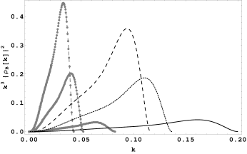
(a) Magnetic density of PMF power spectrum for different values of amplitude and spectral indices.

(b) Lorentz force spectra (black lines) and scalar anisotropic trace-free part (gray lines with points) for different spectral indices.

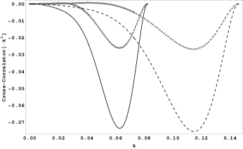
(c) Cross-correlation of $|\rho_{B}\Pi^{(S)}|$ in gray with points and $|\rho_{B}L^{(S)}|$ in black, for different spectral indices.

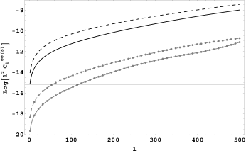
(d) CMB temperature anisotropy angular power spectrum induced by scalar magnetic mode.

Figure 1: Correlators and power spectrum for CMB anisotropies due to a PMF.

The result of the angular power spectrum induced by scalar magnetic perturbations given by eq. (12) is shown in the figure 1(d). Here, the black thick line defines the power spectrum for $n=2$ and the black dashed line for $n=5/2$, both with a strength of $B=1$nG. The gray thick line with points is for $n=2$ and the other one is for $n=5/2$, the gray lines with points are for $B=10$nG.
Acknowledgments. Héctor J. Hortúa acknowledges the IAU-S306 Grant.

References

• [Kahniashvili et al. (2007)] Kahniashvili T., & Ratra B. 2007, Phys. Rev. D, 75, 023002
• [Finelli et al. (2008)] Finelli F., Paci F., & Paoletti D. 2008, Phys. Rev. D, 78, 0233510
• [Yamazaki (2014)] Yamazaki D. G. 2014, Phys. Rev. D, 89, 083528
• [Hortua et al. (2014)] Hortúa H. J., & Castañeda L. 2014, Phys. Rev. D 90, 123520