Multinomial and empirical likelihood under convex constraints: directions of recession, Fenchel duality, perturbations

Abstract

The primal problem of multinomial likelihood maximization restricted to a convex closed subset of the probability simplex is studied. Contrary to widely held belief, a solution of this problem may assign a positive mass to an outcome with zero count. Related flaws in the simplified Lagrange and Fenchel dual problems, which arise because the recession directions are ignored, are identified and corrected.

A solution of the primal problem can be obtained by the PP (perturbed primal) algorithm, that is, as the limit of a sequence of solutions of perturbed primal problems. The PP algorithm may be implemented by the simplified Fenchel dual.

The results permit us to specify linear sets and data such that the empirical likelihood-maximizing distribution exists and is the same as the multinomial likelihood-maximizing distribution. The multinomial likelihood ratio reaches, in general, a different conclusion than the empirical likelihood ratio.

Implications for minimum discrimination information, compositional data analysis, Lindsay geometry, bootstrap with auxiliary information, and Lagrange multiplier test are discussed.

Keywords and phrases: closed multinomial distribution, maximum likelihood, convex set, estimating equations, zero counts, Fenchel dual, El Barmi Dykstra dual, Smith dual, perturbed primal, PP algorithm, epi-convergence, empirical likelihood, Fisher likelihood

AMS 2010 subject classifications: Primary $\mathrm{62H12}$, $\mathrm{62H17}$; secondary $\mathrm{90C46}$

1 Introduction

Zero counts are a source of difficulties in the maximization of the multinomial likelihood for log-linear models. A considerable literature has been devoted to this issue, culminating in the recent papers by Fienberg and Rinaldo [12] and Geyer [14]. In these studies, convex analysis considerations play a key role.

Less well recognized is that the zero counts also cause difficulties in the maximization of the multinomial likelihood under linear constraints, or, in general, when the cell probabilities are restricted to a convex closed subset of the probability simplex; see Section 2 for a formal statement of the considered primal optimization problem $\mathcal{P}$. Though in this case the nature of the difficulties is different than in the log-linear case, the convex analysis considerations are important here as well, because they permit developing a correct solution of $\mathcal{P}$ – one of the main objectives of the present work.

The problem of finding the maximum multinomial likelihood under linear constraints dates back to, at least, Smith [41], and continues through the work of Aitchison and Silvey [4], Gokhale [16], Klotz [26], Haber [19], Stirling [42], Pelz and Good [33], Little and Wu [30], El Barmi and Dykstra [10, 11], to the recent studies by Agresti and Coull [2], Lang [27], and Bergsma et al. [8], among others. Linear constraints on the cell probabilities appear naturally in marginal homogeneity models, isotonic cone models, mean response models, multinomial-Poisson homogeneous models, and many others; cf. Agresti [1], Bergsma et al. [8]. They also arise in the context of estimating equations.

Contrary to widely-held belief, a solution of $\mathcal{P}$ may assign a positive weight to an outcome with zero count; cf. Theorem 2, Examples 3 and 4, as well as the examples in Section 5. This fact also affects the Lagrange and Fenchel dual problems to $\mathcal{P}$.

The restricted maximum of the multinomial likelihood defined through the primal problem $\mathcal{P}$ is not amenable to asymptotic analysis, and the primal form is not ideal for numerical optimization. Thus, it is common to consider the Lagrange dual problem instead of the primal problem. This permits the asymptotic analysis (cf. Aitchison and Silvey [4]), and reduces the dimension of the optimization problem, because the number of linear constraints is usually much smaller than the cardinality of the sample space. Smith [41, Sects. 6, 7] has developed a solution of the Lagrange dual problem, under the hidden assumption that every outcome from the sample space appears in the sample at least once; that is, $\nu>0$, where $\nu$ is the vector of the observed relative frequency of outcomes. The same solution was later considered by several authors; see, in particular, Haber [19, p. 3], Little and Wu [30, p. 88], Lang [27, Sect. 7.1], Bergsma et al. [8, p. 65]. It remained unnoticed that, if the assumption $\nu>0$ is not satisfied, then the solution of Smith’s Lagrange dual problem does not necessarily lead to a solution of the primal problem $\mathcal{P}$.

El Barmi and Dykstra [10] studied the maximization of the multinomial likelihood under more general, convex set constraints, where it is natural to replace the Lagrange duality with the Fenchel duality. When the feasible set is defined by the linear constraints, El Barmi and Dykstra’s (BD) dual $\mathcal{B}$ reduces to Smith’s Lagrange dual. The BD-dual $\mathcal{B}$ leads to a solution of the primal $\mathcal{P}$ if $\nu>0$. The authors overlooked that this is not necessarily the case if a zero count occurs.

Taken together, the decisions obtained from El Barmi and Dykstra’s simplified Fenchel dual $\mathcal{B}$ can be severely compromised. It is thus important to know the correct Fenchel dual $\mathcal{F}$ to $\mathcal{P}$. This is provided by Theorem 6, which also characterizes the solution set of $\mathcal{F}$. It is equally important to know the conditions under which the BD-dual $\mathcal{B}$ leads to a solution of $\mathcal{P}$. The answer is provided by Theorem 16. An analysis of directions of recession is crucial for establishing the theorem.

Since obtaining a solution of the Fenchel dual is numerically demanding, a simple algorithm for solving the primal is proposed. The PP algorithm forms a sequence of perturbed primal problems. Theorem 21 demonstrates that the PP algorithm epi-converges to a solution of $\mathcal{P}$. Even stronger, pointwise convergence can be established for a linear constraint set; see Theorem 22. The convergence theorems imply that the common practice of replacing the zero counts by a small, arbitrary value can be supplanted by a sequence of perturbed primal problems, where the $\delta-$perturbed relative frequency vectors $\nu(\delta)>0$ are such that $\lim_{\delta\searrow 0}\nu(\delta)=\nu$. Because each $\nu(\delta)$ is strictly positive, the PP algorithm can be implemented through the BD-dual to the perturbed primal, by the Fisher scoring algorithm, Gokhale’s algorithm [16], or similar methods.

The findings have implications for the empirical likelihood. Recall that ‘in most settings, empirical likelihood is a multinomial likelihood on the sample’; cf. Owen [32, p. 15]. As the empirical likelihood inner problem $\mathcal{E}$ (cf. Section 9) is a convex optimization problem, it has its Fenchel dual formulation. If the feasible set is linear, then the Fenchel dual to $\mathcal{E}$ is equivalent to El Barmi and Dykstra’s dual $\mathcal{B}$ to $\mathcal{E}$. Thanks to this connection, Theorem 16 provides conditions under which the solution set $S_{\scriptscriptstyle{\mathcal{P}}}$ of the multinomial likelihood primal problem $\mathcal{P}$ and the solution set $S_{\scriptscriptstyle{\mathcal{E}}}$ of the empirical likelihood inner problem $\mathcal{E}$ are the same, and the maximum $\hat{L}$ of the multinomial likelihood is equal to the maximum $\hat{L}_{\scriptscriptstyle{\mathcal{E}}}$ of the empirical likelihood. Consequently:

• If $C$ is an H-set or a Z-set with respect to the type $\nu$ (for the definition, see Section 6), the maximum empirical likelihood does not exist, though the maximum multinomial likelihood exists. The notion of H-set corresponds to the convex hull problem (cf. Owen [31, Sect. 10.4]) and the notion of Z-set corresponds to the zero likelihood problem (cf. Bergsma et al. [7]). By Theorem 16, these are the only ways the empirical likelihood inner problem may fail to have a solution; cf. Section 9.

• If any of conditions (i)–(iv) in Theorem 16(b) are not satisfied, then $\hat{L}_{\scriptscriptstyle{\mathcal{E}}}<\hat{L}$, and the empirical likelihood may lead to different inferential and evidential conclusions than those suggested by the multinomial likelihood.

Fisher’s [13] original concept of the likelihood carries the discordances between the multinomial and empirical likelihoods also into the continuous iid setting; cf. Section 9.1.

The findings also affect other methods, such as the minimum discrimination information, compositional data analysis, Lindsay geometry of multinomial mixtures, bootstrap with auxiliary information, and Lagrange multiplier test, which explicitly or implicitly ignore information about the support and are restricted to the observed outcomes.

1.1 Organization of the paper

The multinomial likelihood primal problem $\mathcal{P}$ and its characterization (cf. Theorem 2) are presented in Section 2. The Fenchel dual problem $\mathcal{F}$ to $\mathcal{P}$ is introduced in Section 3. A Lagrange dual formulation of the convex conjugate (cf. Theorem 5) serves as a ground for Theorem 6, one of the main results, which provides a relation between the solutions of $\mathcal{P}$ and $\mathcal{F}$. If the feasible set $C$ is polyhedral, a solution of $\mathcal{F}$ can be obtained also from a different Lagrange dual to $\mathcal{P}$; cf. Section 3.1. A special case of the single inequality constraint is discussed in detail in Section 3.2, where a flaw in Klotz’s [26] Theorem 1 is noted. In Section 4, El Barmi and Dykstra’s [10] dual $\mathcal{B}$ is recalled; Section 4.1 introduces its special case, the Smith dual problem. Theorem 2.1 of El Barmi and Dykstra [10], and its flaws are presented in Section 5, where they are also illustrated by simple examples. Section 6 studies the scope of validity of the BD-dual $\mathcal{B}$; cf. Theorem 16. Sequential, active-passive dualization is proposed and analyzed in Section 7. Perturbed primal problem $\mathcal{P}_{\delta}$ is introduced in Section 8, where the epi-convergence of a sequence of the perturbed primals for a general, convex $C$, and the pointwise convergence for the linear $C$ are formulated (cf. Theorems 21, 22) and illustrated. Implications of the results for the empirical likelihood method are discussed in Section 9. A brief discussion of implications of the findings for the minimum discrimination information, compositional data analysis, Lindsay geometry of multinomial mixtures, bootstrap with auxiliary information and Lagrange multiplier test is contained in Section 10. Finally, Section 11 comprises detailed proofs of the results.

An R code and data to reproduce the numerical examples can be found in [18].

2 Multinomial likelihood primal problem $\mathcal{P}$

Let $\mathcal{X}$ denote a finite alphabet (sample space) consisting of $m$ letters (outcomes) and $\Delta_{\mathcal{X}}$ denote the probability simplex

$$\Delta_{\mathcal{X}}\triangleq\left\{q\in\mathbb{R}^{m}:\ q\geq 0,\sum q=1\right\};$$

identify $\mathbb{R}^{m}$ with $\mathbb{R}^{\mathcal{X}}$. Suppose that $(n_{i})_{i\in\mathcal{X}}$ is a realization of the closed multinomial distribution $\mathrm{Pr}((n_{i})_{i\in\mathcal{X}};n,q)=n!\prod{q_{i}^{n_{i}}/n_{i}!}$ with parameters $n\in\mathbb{N}$ and $q=(q_{i})_{i\in\mathcal{X}}\in\Delta_{\mathcal{X}}$. Then the multinomial likelihood kernel $L(q)=L_{\nu}(q)\triangleq e^{-n\,\ell(q)}$, where $\ell=\ell_{\nu}:\Delta_{\mathcal{X}}\to\bar{\mathbb{R}}$, Kerridge’s inaccuracy [25], is

$$\ell(q)\triangleq-\left\langle\nu,\log q\right\rangle,$$ (2.1)

and $\nu\triangleq(n_{i}/n)_{i\in\mathcal{X}}$ is the type (the vector of the relative frequency of outcomes). The conventions $\log 0=-\infty$, $0\cdot(-\infty)=0$ apply; $\bar{\mathbb{R}}$ denotes the extended real line $[-\infty,\infty]$ and $\left\langle a,b\right\rangle$ is the scalar product of $a$, $b\in\mathbb{R}^{m}$. Functions and relations on vectors are taken component-wise; for example, $\log q=(\log q_{i})_{i\in\mathcal{X}}$. For $x\in\mathbb{R}^{m}$, $\sum x$ is a shorthand for $\sum_{i\in\mathcal{X}}x_{i}$.

Consider the problem $\mathcal{P}$ of minimization of $\ell$, restricted to a convex closed set $C\subseteq\Delta_{\mathcal{X}}$:

$$\hat{\ell}_{{\scriptscriptstyle{\mathcal{P}}}}\triangleq\inf_{q\in C}\ell(q),\qquad S_{{\scriptscriptstyle{\mathcal{P}}}}\triangleq\{\hat{q}\in C:\ \ell(\hat{q})=\hat{\ell}_{\scriptscriptstyle{\mathcal{P}}}\}. \mathcal{P}$$ ()

The goal is to find the solution set $S_{{\scriptscriptstyle{\mathcal{P}}}}$ as well as the infimum $\hat{\ell}_{\scriptscriptstyle{\mathcal{P}}}$ of the objective function $\ell$ over $C$. The problem $\mathcal{P}$ will be called the multinomial likelihood primal problem, or primal, for short.

Special attention is paid to the class of polyhedral feasible sets $C$

$$C=\{q\in\Delta_{\mathcal{X}}:\left\langle q,u_{h}\right\rangle\leq 0\text{ for }h=1,2,\dots,r\},$$ (2.2)

or to its subclass of sets $C$ given by (a finite number of) linear equality constraints

$$C=\{q\in\Delta_{\mathcal{X}}:\left\langle q,u_{h}\right\rangle=0\text{ for }h=1,2,\dots,r\},$$ (2.3)

where $u_{h}$ are vectors from $\mathbb{R}^{m}$. These feasible sets are particularly interesting from the applied point of view and permit to establish stronger results.

Without loss of generality it is assumed that $\mathcal{X}$ is the support $\operatorname{supp}(C)$ of $C$, that is, for every $i\in\mathcal{X}$ there is $q\in C$ with $q_{i}>0$; in other words, the structural zeros (cf. Baker et al. [6, p. 34]) are excluded. Due to the convexity of $C$ this is equivalent to the existence of $q\in C$ with $q>0$. Under this assumption, Theorem 2 gives a basic characterization of the solution set of $\mathcal{P}$. Before stating it, some useful notions are introduced.

Definition 1.

For a type $\nu$ (or, more generally, for any $\nu\in\Delta_{\mathcal{X}}$), the active and passive alphabets are

$$\mathcal{X}^{a}=\mathcal{X}^{a}_{\nu}\triangleq\{i\in\mathcal{X}:\nu_{i}>0\}\qquad\text{and}\qquad\mathcal{X}^{p}=\mathcal{X}^{p}_{\nu}\triangleq\{i\in\mathcal{X}:\nu_{i}=0\}.$$

The elements of $\mathcal{X}^{a},\mathcal{X}^{p}$ are called active, passive letters, respectively.

Put $m_{a}\triangleq\operatorname{card}\mathcal{X}^{a}>0$, $m_{p}\triangleq\operatorname{card}\mathcal{X}^{p}\geq 0$. Let $\pi^{a}:\mathbb{R}^{m}\to\mathbb{R}^{m_{a}}$, $\pi^{p}:\mathbb{R}^{m}\to\mathbb{R}^{m_{p}}$ be the natural projections; identify $\mathbb{R}^{m_{a}}$ with $\mathbb{R}^{\mathcal{X}^{a}}$ and $\mathbb{R}^{m_{p}}$ with $\mathbb{R}^{\mathcal{X}^{p}}$. Note that if $\mathcal{X}^{p}=\emptyset$ then $m_{p}=0$ and $\mathbb{R}^{m_{p}}=\{0\}$. For $x\in\mathbb{R}^{m}$, $x^{a}$ and $x^{p}$ are the shorthands for $\pi^{a}(x)$ and $\pi^{p}(x)$, respectively. (If no ambiguity can occur, the elements of $\mathbb{R}^{m_{a}},\mathbb{R}^{m_{p}}$ will be denoted also by $x^{a},x^{p}$.) Identify $\mathbb{R}^{m}$ with $\mathbb{R}^{m_{a}}\times\mathbb{R}^{m_{p}}$, so that it is possible to write $x=(x^{a},x^{p})$ for every $x\in\mathbb{R}^{m}$. Finally, for a subset $M$ of $\mathbb{R}^{m}$ and $x\in M$ let

$$M^{a}\triangleq\pi^{a}(M)\qquad\text{and}\qquad M^{a}(x^{p})\triangleq\{x^{a}\in\mathbb{R}^{m_{a}}:(x^{a},x^{p})\in M\}$$

be the active projection and the $x^{p}$-slice of $M$; analogously define $M^{p}$ and $M^{p}(x^{a})$.

Theorem 2 (Primal problem).

Let $\nu\geq 0$ be from $\Delta_{\mathcal{X}}$. Let $C$ be a convex closed subset of $\Delta_{\mathcal{X}}$ with support $\mathcal{X}$. Then $\hat{\ell}_{\scriptscriptstyle{\mathcal{P}}}$ is finite, $S_{{\scriptscriptstyle{\mathcal{P}}}}$ is compact and there is $\hat{q}^{a}_{\scriptscriptstyle{\mathcal{P}}}\in C^{a}$, $\hat{q}^{a}_{\scriptscriptstyle{\mathcal{P}}}>0$, such that

$$S_{{\scriptscriptstyle{\mathcal{P}}}}=\{\hat{q}^{a}_{\scriptscriptstyle{\mathcal{P}}}\}\times C^{p}(\hat{q}^{a}_{\scriptscriptstyle{\mathcal{P}}}).$$

Moreover,

1. If $\sum\hat{q}^{a}_{\scriptscriptstyle{\mathcal{P}}}=1$ then $C^{p}(\hat{q}^{a}_{\scriptscriptstyle{\mathcal{P}}})=\{0^{p}\}$ and $S_{{\scriptscriptstyle{\mathcal{P}}}}=\{(\hat{q}^{a}_{\scriptscriptstyle{\mathcal{P}}},0^{p})\}$ is a singleton.

2. If $\sum\hat{q}^{a}_{\scriptscriptstyle{\mathcal{P}}}<1$ then $0^{p}\not\in C^{p}(\hat{q}^{a}_{\scriptscriptstyle{\mathcal{P}}})$, and $S_{\scriptscriptstyle{\mathcal{P}}}$ is a singleton if and only if the $\hat{q}^{a}_{\scriptscriptstyle{\mathcal{P}}}$-slice $C^{p}(\hat{q}^{a}_{\scriptscriptstyle{\mathcal{P}}})$ of $C$ is a singleton.

Thus the primal has always a solution $\hat{q}_{{\scriptscriptstyle{\mathcal{P}}}}$. Its active coordinates $\hat{q}^{a}_{\scriptscriptstyle{\mathcal{P}}}$ are unique and the passive coordinates $\hat{q}^{p}_{\scriptscriptstyle{\mathcal{P}}}$ are arbitrary such that $\hat{q}_{\scriptscriptstyle{\mathcal{P}}}\in C$. It is worth stressing that $C^{p}(\hat{q}^{a}_{\scriptscriptstyle{\mathcal{P}}})$ need not be equal to $\{0^{p}\}$, that is, a solution of $\mathcal{P}$ may put positive mass to passive letter(s). The following couple of simple examples illustrates the points; see also the examples in Section 5. Hereafter $X$ denotes a random variable supported on $\mathcal{X}$.

Example 3.

Take $\mathcal{X}=\{-1,0,1\}$ and $C=\{q\in\Delta_{\mathcal{X}}:\ \operatorname{E}_{q}(X^{2})=\sum_{i\in\mathcal{X}}i^{2}q_{i}=1/2\}$. Let $\nu=(0,1,0)$, so that $\mathcal{X}^{a}=\{0\}$ and $\mathcal{X}^{p}=\{-1,1\}$. Then $C=\{q\in\Delta_{\mathcal{X}}:\ q_{0}=1/2\}$, the minimum of $\ell$ over $C$ is $\hat{\ell}_{\scriptscriptstyle{\mathcal{P}}}{}=\log 2$, and $S_{\scriptscriptstyle{\mathcal{P}}}=C$. Here, $\hat{q}^{a}_{\scriptscriptstyle{\mathcal{P}}}=1/2$ is (trivially) unique and $C^{p}(\hat{q}^{a}_{\scriptscriptstyle{\mathcal{P}}})=\{(a,1/2-a):a\in[0,1/2]\}$.

Example 4.

Motivated by Wets [43, p. 88], let $\mathcal{X}=\{1,2,3\}$, $C=\{q\in\Delta_{\mathcal{X}}:q_{1}\leq q_{2}\leq q_{3}\}$ and $\nu=(0,1,0)$. Then $\mathcal{X}^{a}=\{2\}$, $\mathcal{X}^{p}=\{1,3\}$. Since $S_{\scriptscriptstyle{\mathcal{P}}}=\{(0,1,1)/2\}$, the positive weight $1/2$ is assigned to the passive, unobserved letter $3$.

The Fisher scoring algorithm which is commonly used to solve $\mathcal{P}$ when $C$ is a linear set may fail to converge when the zero counts are present; cf. Stirling [42]. Other numerical methods, such as the augmented Lagrange multiplier methods, which are used to solve the convex optimization problem under polyhedral and/or linear $C$ may have difficulties to cope with large $m$. Thus, it is desirable to approach $\mathcal{P}$ also from another direction.

3 Fenchel dual problem $\mathcal{F}$ to $\mathcal{P}$

Consider the Fenchel dual problem $\mathcal{F}$ to the primal $\mathcal{P}$:

$$\hat{\ell}_{\scriptscriptstyle{\mathcal{F}}}\triangleq\inf_{y\in C^{\ast}}\ell^{\ast}(-y),\qquad S_{{\scriptscriptstyle{\mathcal{F}}}}\triangleq\{\hat{y}\in C^{\ast}:\ \ell^{\ast}(-\hat{y})=\hat{\ell}_{\scriptscriptstyle{\mathcal{F}}}\}, \mathcal{F}$$ ()

where

$$C^{\ast}\triangleq\{y\in\mathbb{R}^{m}:\left\langle y,q\right\rangle\leq 0\text{ for every }q\in C\}$$

is the polar cone of $C$ and

$$\ell^{\ast}:\mathbb{R}^{m}\to\bar{\mathbb{R}},\qquad\ell^{\ast}(z)\triangleq\sup_{q\in\Delta_{\mathcal{X}}}(\left\langle q,z\right\rangle-\ell(q))$$

is the convex conjugate of $\ell$ (in fact, the convex conjugate of $\tilde{\ell}:\mathbb{R}^{m}\to\bar{\mathbb{R}}$ given by $\tilde{\ell}(x)=\ell(x)$ for $x\in\Delta_{\mathcal{X}}$ and $\tilde{\ell}(x)=\infty$ otherwise).

The Fenchel dual $\mathcal{F}$ is often more tractable than the primal $\mathcal{P}$, in particular when $C$ is given by linear equality and/or inequality constraints. This is the case of the models for contingency tables, mentioned in Introduction. Also an estimating equations model $C_{\Theta}$ leads to a linear feasible set $C_{\theta}$, when $\theta\in\Theta$ is fixed. The model is $C_{\Theta}\triangleq\bigcup_{\theta\in\Theta}C_{\theta}$, where

$$C_{\theta}\triangleq\bigcap_{h=1}^{r}\left\{q\in\Delta_{\mathcal{X}}:\left\langle q,u_{h}(\theta)\right\rangle=0\right\},$$ (3.1)

and $u_{h}:\Theta\rightarrow\mathbb{R}^{m}$, $h=1,2,\dots,r$, are the estimating functions. There $\theta\in\Theta\subseteq\mathbb{R}^{d}$ and $d$ need not be equal to $r$. Since $r$ is usually much smaller than $m$, $\mathcal{F}$ may be easier to solve numerically than $\mathcal{P}$.

Observe that the convex conjugate itself is defined through an optimization problem, the convex conjugate primal problem (cc-primal, for short), whose solution set is

$$S_{{cc}}(z)\triangleq\{q\in\Delta_{\mathcal{X}}:\left\langle q,z\right\rangle-\ell(q)=\ell^{\ast}(z)\}.$$ (3.2)

The structure of $S_{{cc}}(z)$ is described by Proposition 40. The conjugate $\ell^{\ast}$ can be evaluated by means of the Lagrange duality, where the Lagrange function is

$$K_{z}(x,\mu)=\left\langle x,z\right\rangle-\ell(x)-\mu\left(\sum x-1\right).$$

It holds that (cf. Lemma 38)

$$\ell^{\ast}(z)=\inf_{\mu\in\mathbb{R}}k_{z}(\mu),\qquad\text{where}\quad k_{z}(\mu)=\sup_{x\geq 0}K_{z}(x,\mu).$$

For every $\mu\in\mathbb{R}$ and $a,b\in\mathbb{R}^{m_{a}}$, $a>0$, $b>-\mu$, define

$$I_{\mu}(a\,\|\,b)\triangleq\left\langle a,\log\frac{a}{\mu+b}\right\rangle.$$

Theorem 5 (Convex conjugate by Lagrange duality).

Let $\nu\in\Delta_{\mathcal{X}}$ and $z\in\mathbb{R}^{m}$. Then

$$\ell^{\ast}(z)=-1+\hat{\mu}(z)+I_{\hat{\mu}(z)}(\nu^{a}\,\|\,-z^{a}),$$

where

$$\hat{\mu}(z)\triangleq\max\{\bar{\mu}(z^{a}),\max(z^{p})\},$$ (3.3)

and $\bar{\mu}(z^{a})$ is the unique solution of

$$\sum\frac{\nu^{a}}{\mu-z^{a}}=1,\qquad\mu\in(\max(z^{a}),\infty).$$ (3.4)

The key point is that the $\bar{\mu}(z^{a})$, which solves (3.4), is not always the $\hat{\mu}(z)$ which minimizes $k_{z}(\mu)$. They are the same if and only if $\bar{\mu}(z^{a})\geq\max(z^{p})$. As it will be seen in Theorem 6, if $z\in S_{\scriptscriptstyle{\mathcal{F}}}$ then this inequality decides whether the solution of primal $\mathcal{P}$ is supported only on the active letters, or some probability mass is placed also to the passive letter(s).

Theorem 5 serves as a foundation for Theorem 6, which states the relation between the Fenchel dual and the primal.

Theorem 6 (Relation between $\mathcal{F}$ and $\mathcal{P}$).

Let $\nu,C,\hat{q}^{a}_{\scriptscriptstyle{\mathcal{P}}}$ be as in Theorem 2. Then

$$\hat{\ell}_{\scriptscriptstyle{\mathcal{F}}}=-\hat{\ell}_{\scriptscriptstyle{\mathcal{P}}},$$

$S_{\scriptscriptstyle{\mathcal{F}}}$ is a nonempty convex compact set and $\hat{\mu}(-\hat{y}_{\scriptscriptstyle{\mathcal{F}}})=1$ for every $\hat{y}_{\scriptscriptstyle{\mathcal{F}}}\in S_{\scriptscriptstyle{\mathcal{F}}}$. Moreover, if we put

$$\hat{y}^{a}_{\scriptscriptstyle{\mathcal{F}}}\triangleq\frac{\nu^{a}}{\hat{q}^{a}_{\scriptscriptstyle{\mathcal{P}}}}-1^{a},$$ (3.5)

then $(\hat{y}^{a}_{\scriptscriptstyle{\mathcal{F}}},-1^{p})\in S_{\scriptscriptstyle{\mathcal{F}}}$ and the following hold:

1. If $\sum\hat{q}^{a}_{\scriptscriptstyle{\mathcal{P}}}=1$ then $\bar{\mu}(-\hat{y}^{a}_{\scriptscriptstyle{\mathcal{F}}})=1$ and

   $$S_{\scriptscriptstyle{\mathcal{F}}}=\{\hat{y}^{a}_{\scriptscriptstyle{\mathcal{F}}}\}\times\{y^{p}\in C^{\ast p}(\hat{y}^{a}_{\scriptscriptstyle{\mathcal{F}}}):\min(y^{p})\geq-1\}.$$

2. If $\sum\hat{q}^{a}_{\scriptscriptstyle{\mathcal{P}}}<1$ then $\bar{\mu}(-\hat{y}^{a}_{\scriptscriptstyle{\mathcal{F}}})<1$ and

   $$S_{\scriptscriptstyle{\mathcal{F}}}=\{\hat{y}^{a}_{\scriptscriptstyle{\mathcal{F}}}\}\times\{y^{p}\in C^{\ast p}(\hat{y}^{a}_{\scriptscriptstyle{\mathcal{F}}}):\min(y^{p})=-1\}.$$

Thus, in the active coordinates, the solution of $\mathcal{F}$ is unique and is related to $\hat{q}^{a}_{\scriptscriptstyle{\mathcal{P}}}$ by (3.5). Together with Theorem 2 this yields

$$S_{\scriptscriptstyle{\mathcal{P}}}=\left\{\frac{\nu^{a}}{1+\hat{y}^{a}_{\scriptscriptstyle{\mathcal{F}}}}\right\}\times C^{p}\left(\frac{\nu^{a}}{1+\hat{y}^{a}_{\scriptscriptstyle{\mathcal{F}}}}\right).$$

The structure of the solution set of $\mathcal{F}$ in the passive letters is determined by the relation of $\bar{\mu}(-\hat{y}^{a}_{\scriptscriptstyle{\mathcal{F}}})$ to $1=\hat{\mu}(-\hat{y}_{\scriptscriptstyle{\mathcal{F}}})$.

In the case (a), $\bar{\mu}(-\hat{y}^{a}_{\scriptscriptstyle{\mathcal{F}}})=\hat{\mu}(-\hat{y}_{\scriptscriptstyle{\mathcal{F}}})$, and the passive projections $\hat{y}^{p}_{\scriptscriptstyle{\mathcal{F}}}$ of the solutions satisfy $\hat{y}^{p}_{\scriptscriptstyle{\mathcal{F}}}\geq-1$. Then it suffices to solve the primal solely in the active letters and $S_{\scriptscriptstyle{\mathcal{P}}}$ is a singleton. This happens for instance if $\nu>0$.

In the case (b), $\bar{\mu}(-\hat{y}^{a}_{\scriptscriptstyle{\mathcal{F}}})<\hat{\mu}(-\hat{y}_{\scriptscriptstyle{\mathcal{F}}})$, and $\hat{y}^{p}_{\scriptscriptstyle{\mathcal{F}}}$ satisfy $\min(\hat{y}^{p}_{\scriptscriptstyle{\mathcal{F}}})=-1$. Then every solution of the primal assigns the positive probability to at least one passive letter.

To sum up, the Fenchel dual problem, once solved, permits to find $\hat{q}^{a}_{\scriptscriptstyle{\mathcal{P}}}$ through (3.5) and this way it incorporates $C^{\ast}$ into $\hat{q}^{a}_{\scriptscriptstyle{\mathcal{P}}}$. In the case of linear or polyhedral $C$ the dual may reduce dimensionality of the optimization problem, yet the numerical solution of $\mathcal{F}$ is somewhat hampered by the need to obey (3.3). Moreover, $\hat{q}^{p}_{\scriptscriptstyle{\mathcal{P}}}$ remains to be found; in this respect see Proposition 51.

3.1 Polyhedral and linear $C$

In the polyhedral case (2.2)

$$C=\{q\in\Delta_{\mathcal{X}}:\left\langle q,u_{h}\right\rangle\leq 0\text{ for }h=1,2,\dots,r\},$$

a solution of the Fenchel dual $\mathcal{F}$ can also be obtained from the saddle points of the following Lagrange function

$$L(q,\alpha)\triangleq-\sum_{h}\alpha_{h}\left\langle q,u_{h}\right\rangle-\ell(q)\qquad(q\in\Delta_{\mathcal{X}},\alpha\in\mathbb{R}^{r}_{+}).$$

Indeed, it holds that

$$\hat{\ell}_{\scriptscriptstyle{\mathcal{F}}}=\adjustlimits{\inf}_{\alpha\geq 0}{\sup}_{q\in\Delta_{\mathcal{X}}}L(q,\alpha)=\adjustlimits{\sup}_{q\in\Delta_{\mathcal{X}}}{\inf}_{\alpha\geq 0}L(q,\alpha)=-\hat{\ell}_{\scriptscriptstyle{\mathcal{P}}}.$$

Hence $(\hat{q},\hat{\alpha})$ is a saddle point of $L(q,\alpha)$ if and only if $\hat{q}\in S_{\scriptscriptstyle{\mathcal{P}}}$ and $\sum_{h}\hat{\alpha}_{h}u_{h}\in S_{\scriptscriptstyle{\mathcal{F}}}$; cf. Bertsekas [9, Prop. 2.6.1].

The vectors from $S_{\scriptscriptstyle{\mathcal{F}}}$ of the form $\sum_{h}\hat{\alpha}_{h}u_{h}$ will be called the base solutions of $\mathcal{F}$. From the Farkas lemma (cf. Bertsekas [9, Prop. 3.2.1]) and the monotonicity of $\ell^{\ast}$ (Lemma 41) it follows that, for a polyhedral $C$, there always exists a base solution, and every solution of $\mathcal{F}$ is a sum of a base solution and a vector from $\mathbb{R}^{m}_{-}\triangleq\{z\in\mathbb{R}^{m}:z\leq 0\}$; that is,

$$S_{\scriptscriptstyle{\mathcal{F}}}=\left\{\hat{y}_{\scriptscriptstyle{\mathcal{F}}}{}+(0^{a},z^{p}):\hat{y}_{\scriptscriptstyle{\mathcal{F}}}{}\text{ is a base solution, }z^{p}\leq 0,\ \hat{y}_{\scriptscriptstyle{\mathcal{F}}}^{p}+z^{p}\geq-1\right\}.$$

There may exist many base solutions. However, if $u_{1}^{a},\dots,u_{r}^{a}$ are linearly independent then the base solution is unique, since then the system of equations $\sum_{h}\hat{\alpha}_{h}u_{h}^{a}=\hat{y}_{\scriptscriptstyle{\mathcal{F}}}^{a}$ has a unique solution $\hat{\alpha}$.

Analogous claim holds for a linear $C$ (cf. (2.3)), just in this case $\alpha\in\mathbb{R}^{r}$, by the Farkas lemma.

3.2 Single inequality constraint and Klotz’s Theorem 1

To illustrate the base solution in connection with Theorem 6, consider

$$C=\{q\in\Delta_{\mathcal{X}}:\left\langle q,u\right\rangle\leq 0\},$$

given by a single inequality constraint. By the Farkas lemma, $C^{\ast}=\{\alpha u:\alpha\geq 0\}+\mathbb{R}^{m}_{-}$. If $u^{p}\geq 0$ the case (a) of Theorem 6 applies (for if not, there is a base solution $\hat{\alpha}_{\scriptscriptstyle{\mathcal{F}}}u$ and, by Theorem 6(b), $\min(\hat{\alpha}_{\scriptscriptstyle{\mathcal{F}}}u^{p})$ should be $-1$; this is not possible since $\min(\hat{\alpha}_{\scriptscriptstyle{\mathcal{F}}}u^{p})\geq 0$).

Assume that $\min(u^{p})<0$ and the case (b) of Theorem 6 applies. Take any base solution $\hat{\alpha}_{\scriptscriptstyle{\mathcal{F}}}u$. Then, by Theorem 6(b), $\min(\hat{\alpha}_{\scriptscriptstyle{\mathcal{F}}}u^{p})=-1$; so

$$\hat{\alpha}_{\scriptscriptstyle{\mathcal{F}}}=-\frac{1}{\min(u^{p})}\qquad\text{and}\qquad\hat{q}^{a}_{\scriptscriptstyle{\mathcal{P}}}=\frac{\nu^{a}}{1-\frac{u^{a}}{\min(u^{p})}}\,.$$ (3.6)

Further, by Theorem 2, $\hat{q}^{p}_{\scriptscriptstyle{\mathcal{P}}}$ is arbitrary from $C^{p}(\hat{q}^{a}_{\scriptscriptstyle{\mathcal{P}}})$. If $u^{p}$ attains the minimum at a single letter, then the solution of the primal $\mathcal{P}$ is always unique.

To sum up, the case (b) of Theorem 6 happens if and only if

$$\min(u^{p})<0\qquad\text{and}\qquad\sum\frac{\nu^{a}}{1-\frac{1}{\min(u^{p})}u^{a}}<1.$$ (3.7)

The primal problem $\mathcal{P}$ with this $C$ was considered by Klotz [26]. Theorem 1 of [26] asserts that the solution of $\mathcal{P}$ takes the form

$$\hat{q}_{K}\triangleq\frac{\nu}{1+\hat{\alpha}_{K}u}$$

if $\left\langle\nu,u\right\rangle>0$ and $\min(u^{a})<0$; see Klotz’s condition (3.1b). There, $\hat{\alpha}_{K}$ is the unique root of

$$\sum\frac{\nu}{1+\alpha u}=1\qquad\text{such that}\quad\alpha\in(0,-1/\min(u^{a})).$$

Thus, under Klotz’s condition (3.1b), the solution of $\mathcal{P}$ should assign zero weight to any passive letter. This is not the case, as the following example demonstrates.

Example 7 (Base solution of $\mathcal{F}$, one inequality constraint).

Take $\mathcal{X}=\{-2,-1,0,$ $1,2\}$, $u=(-2,-1,0,1,2)$ and $\nu=(0,3,0,0,7)/10$. Here Klotz’s condition (3.1b) is satisfied and an easy computation yields $\hat{\alpha}_{K}=11/20$; thus $\hat{q}_{K}=(0,2,0,0,1)/3$ and $\ell(\hat{q}_{K})=0.890668$. However, $\hat{q}_{\scriptscriptstyle{\mathcal{P}}}=(1,12,0,0,7)/20$, so a positive mass is placed also to the passive letter $-2$; $\ell(\hat{q}_{\scriptscriptstyle{\mathcal{P}}})=0.888123$. Since $\min(u^{p})=-2$ and $\sum\hat{q}^{a}_{\scriptscriptstyle{\mathcal{P}}}<1$, the condition (3.7) is satisfied and $\hat{q}^{a}_{\scriptscriptstyle{\mathcal{P}}}$ is just that given by (3.6).

In a similar way it is possible to analyze a single equality constraint. For more than one equality/inequality constraint the condition guaranteeing that $\sum\hat{q}^{a}_{\scriptscriptstyle{\mathcal{P}}}<1$ cannot be given in such a simple form as (3.7).

4 El Barmi-Dykstra dual problem $\mathcal{B}$ to $\mathcal{P}$

El Barmi and Dykstra [10] consider a simplified Fenchel dual problem $\mathcal{B}$ (the BD-dual, for short)

$$\hat{\ell}_{{\scriptscriptstyle{\mathcal{B}}}}\triangleq\inf_{y\in C^{\ast}}{\ell^{\ast}_{\scriptscriptstyle{\mathcal{B}}}}(y),\qquad S_{{\scriptscriptstyle{\mathcal{B}}}}\triangleq\{\hat{y}\in C^{\ast}:{\ell^{\ast}_{\scriptscriptstyle{\mathcal{B}}}}(\hat{y})=\hat{\ell}_{\scriptscriptstyle{\mathcal{B}}}\}, \mathcal{B}$$ ()

where

$${\ell^{\ast}_{\scriptscriptstyle{\mathcal{B}}}}:\mathbb{R}^{m}\to\bar{\mathbb{R}},\qquad{\ell^{\ast}_{\scriptscriptstyle{\mathcal{B}}}}(y)\triangleq\begin{cases}I_{1}(\nu^{a}\,\|\,y^{a})=\left\langle\nu^{a},\log\dfrac{\nu^{a}}{1+y^{a}}\right\rangle&\text{if }y^{a}>-1,\\ \infty&\text{otherwise},\end{cases}$$

will be called the BD conjugate of $\ell$. Note that the BD-dual $\mathcal{B}$ is easier to solve than $\mathcal{F}$, as in the former $\hat{\mu}$ is fixed to $1$.

If $C$ is polyhedral then, in analogy with the concept of the base solution of $\mathcal{F}$, the vectors from $S_{\scriptscriptstyle{\mathcal{B}}}$ of the form $\sum\hat{\alpha}_{{\scriptscriptstyle{\mathcal{B}}}{},h}u_{h}$ are called the base solutions of $\mathcal{B}$. As above, every solution of $\mathcal{B}$ can in this case be written as a sum of a base solution and a vector from $\mathbb{R}^{m}_{-}$.

4.1 Smith dual problem

By the Farkas lemma, for the feasible set $C=\{q\in\Delta_{\mathcal{X}}:\left\langle q,u_{h}\right\rangle=0,h=1,2,\dots,r\}$ given by $r$ linear equality constraints, the polar cone is ${C}^{\ast}=\{y=\sum_{h}\alpha_{h}u_{h}:\alpha\in\mathbb{R}^{r}\}+\mathbb{R}^{m}_{-}$. Then the BD-dual becomes

$$\inf_{\alpha\in\mathbb{R}^{r}}\,I_{1}\left(\nu^{a}\,\Bigl{\|}\,\sum_{h}\alpha_{h}u^{a}_{h}\right),$$ (4.1)

which is (equivalent to) the simplified Lagrange dual problem (the Smith dual, for short) considered by Smith [41, Sect. 6] and many other authors; see, in particular, Haber [19, p. 3], Little and Wu [30, p. 88], Lang [27, Sect. 7.1], and Bergsma et al. [8, p. 65]. It is worth noting that (4.2) is an unconstrained optimization problem.

5 Flaws of BD-dual $\mathcal{B}$

In  [10, Thm. 2.1] El Barmi and Dykstra state the following relationship between $\mathcal{P}$ and $\mathcal{B}$.

Theorem 8 (Theorem 2.1 of [10]).

Let $C$ be a convex closed subset of $\Delta_{\mathcal{X}}$.

• ($\mathcal{B}\rightarrow\mathcal{P}$): If $\hat{\ell}_{\scriptscriptstyle{\mathcal{B}}}$ is finite, then $S_{\scriptscriptstyle{\mathcal{B}}}$ is nonempty and $\hat{\ell}_{\scriptscriptstyle{\mathcal{B}}}=-\hat{\ell}_{\scriptscriptstyle{\mathcal{P}}}$. Moreover, for every $\hat{y}_{\scriptscriptstyle{\mathcal{B}}}\in S_{\scriptscriptstyle{\mathcal{B}}}$, $\tilde{q}_{\scriptscriptstyle{\mathcal{B}}}\triangleq\frac{\nu}{1+\hat{y}_{\scriptscriptstyle{\mathcal{B}}}}$ belongs to $S_{\scriptscriptstyle{\mathcal{P}}}$.

• ($\mathcal{P}\rightarrow\mathcal{B}$): If $\hat{\ell}_{\scriptscriptstyle{\mathcal{P}}}$ is finite, then $\hat{\ell}_{\scriptscriptstyle{\mathcal{B}}}=-\hat{\ell}_{\scriptscriptstyle{\mathcal{P}}}$. Moreover, if $\hat{q}_{\scriptscriptstyle{\mathcal{P}}}\in S_{\scriptscriptstyle{\mathcal{P}}}$, then $\tilde{y}_{\scriptscriptstyle{\mathcal{B}}}\triangleq\frac{\nu}{\hat{q}_{\scriptscriptstyle{\mathcal{P}}}}-1$ belongs to $S_{\scriptscriptstyle{\mathcal{B}}}$. (There, $0/0=0$ convention applies).

Though $\hat{\ell}_{\scriptscriptstyle{\mathcal{P}}}$ is always finite, $\hat{\ell}_{\scriptscriptstyle{\mathcal{B}}}$ may be infinite, leaving the solution set $S_{\scriptscriptstyle{\mathcal{P}}}$ inaccessible through ($\mathcal{B}\rightarrow\mathcal{P}$) of [10, Thm. 2.1]. Moreover, the claims ($\mathcal{B}\rightarrow\mathcal{P}$) and ($\mathcal{P}\rightarrow\mathcal{B}$) of the theorem are not always true. In fact, there are three possibilities:

1. $\hat{\ell}_{{\scriptscriptstyle{\mathcal{B}}}}=-\infty$;

2. $\hat{\ell}_{{\scriptscriptstyle{\mathcal{B}}}}$ is finite, but there is a BD-duality gap, that is, $\hat{\ell}_{{\scriptscriptstyle{\mathcal{B}}}}<-\hat{\ell}_{\scriptscriptstyle{\mathcal{P}}}$;

3. $\hat{\ell}_{{\scriptscriptstyle{\mathcal{B}}}}=-\hat{\ell}_{{\scriptscriptstyle{\mathcal{P}}}}$ (no BD-duality gap).

To illustrate them, we give below six simple examples: one where the BD-duality works and the other five where it fails. In Examples 9, LABEL:E:E, LABEL:E:Z, LABEL:E:gap the set $C$ is linear, whereas Example 11 presents a nonlinear $C$, and in Example 12 the set $C$ is defined by linear inequalities.

Example 9 (No BD-duality gap).

Let $\mathcal{X}=\{-1,0,1\}$ and $C=\{q\in\Delta_{\mathcal{X}}:\mathrm{E}_{q}X=0\}$; that is, $C$ is given by (2.3) with $u=(-1,0,1)$. Let $\nu=(1,0,1)/2$. Thus $\mathcal{X}^{a}=\{-1,1\}$, $\mathcal{X}^{p}=\{0\}$, and $C^{a}(0^{p})=\{(1,1)/2\}$. By the Farkas lemma, $C^{\ast}=\{y=\alpha u:\alpha\in\mathbb{R}\}+\mathbb{R}^{3}_{-}$. For the considered optimization problems, the following hold:

• $\mathcal{P}$: $S_{\scriptscriptstyle{\mathcal{P}}}=\{(1,0,1)/2\}$ and $\hat{\ell}_{\scriptscriptstyle{\mathcal{P}}}=\log 2$.

• $\mathcal{F}$: Since $\hat{\alpha}_{\scriptscriptstyle{\mathcal{F}}}=0$, the base solution of $\mathcal{F}$ is $(0,0,0)$ and $\hat{\ell}_{\scriptscriptstyle{\mathcal{F}}}=-\log 2$. Further, (3.5) implies that $\hat{q}^{a}_{\scriptscriptstyle{\mathcal{P}}}=\nu^{a}/(1+\hat{y}^{a}_{\scriptscriptstyle{\mathcal{F}}})$; thus, $\hat{q}^{a}_{\scriptscriptstyle{\mathcal{P}}}=\nu^{a}$.

In this setting, no BD-duality gap occurs:

• $\mathcal{B}$$\rightarrow$$\mathcal{P}$: ${\ell^{\ast}_{\scriptscriptstyle{\mathcal{B}}}}(\alpha u)\propto-1/2[\log(1-\alpha)+\log(1+\alpha)]$. Thus $\hat{\alpha}_{\scriptscriptstyle{\mathcal{B}}}=0$, $\hat{\ell}_{\scriptscriptstyle{\mathcal{B}}}=-\log 2=-\hat{\ell}_{\scriptscriptstyle{\mathcal{P}}}$. Since $\tilde{q}_{\scriptscriptstyle{\mathcal{B}}}=(1,0,1)/2$, it indeed solves $\mathcal{P}$.

• $\mathcal{P}$$\rightarrow$$\mathcal{B}$: $\hat{\ell}_{\scriptscriptstyle{\mathcal{B}}}=-\hat{\ell}_{\scriptscriptstyle{\mathcal{P}}}$ by the previous case. Since the base solution of $\mathcal{B}$ is $(0,0,0)$ and $\tilde{y}_{\scriptscriptstyle{\mathcal{B}}}=(0,0,0)$, $\tilde{y}_{\scriptscriptstyle{\mathcal{B}}}\in S_{\scriptscriptstyle{\mathcal{B}}}$.

Example 10 (name=H-set, label=E:E).

Let $\mathcal{X}$, $C$ be as in Example 9 and $\nu=(1,0,0)$. Thus $\mathcal{X}^{a}=\{-1\}$, $\mathcal{X}^{p}=\{0,1\}$, and $C^{a}(0^{p})=\emptyset$.

• $\mathcal{P}$: $S_{\scriptscriptstyle{\mathcal{P}}}=\{(1,0,1)/2\}$ and $\hat{\ell}_{\scriptscriptstyle{\mathcal{P}}}=\log 2$.

• $\mathcal{F}$: Since $\hat{\alpha}_{\scriptscriptstyle{\mathcal{F}}}=-1$, the base solution of $\mathcal{F}$ is $(1,0,-1)$ and $\hat{\ell}_{\scriptscriptstyle{\mathcal{F}}}=-\log 2$. Thus, from (3.5) it follows that $\hat{q}^{a}_{\scriptscriptstyle{\mathcal{P}}}=(1/2)$.

• $\mathcal{B}$$\rightarrow$$\mathcal{P}$: ${\ell^{\ast}_{\scriptscriptstyle{\mathcal{B}}}}(\alpha u)\propto-\log(1-\alpha)$, which does not have finite infimum.

• $\mathcal{P}$$\rightarrow$$\mathcal{B}$: $\hat{\ell}_{\scriptscriptstyle{\mathcal{B}}}$ is not finite and $S_{\scriptscriptstyle{\mathcal{B}}}=\emptyset$. Thus $\tilde{y}_{\scriptscriptstyle{\mathcal{B}}}=(1,0,-1)\not\in S_{\scriptscriptstyle{\mathcal{B}}}$.

Example 11 (nonlinear $C$, H-set).

Let $\mathcal{X}=\{2,3,4\}$, $C=\{q\in\Delta_{\mathcal{X}}:\sum_{i\in\mathcal{X}}i\,q^{2}_{i}\leq 1\}$, and $\nu=(1,0,0)$. Thus $\mathcal{X}^{a}=\{2\}$, $\mathcal{X}^{p}=\{3,4\}$, and $C^{a}(0^{p})=\emptyset$.

• $\mathcal{P}$: Write $C=\bigcup_{k\in[0,1]}C_{k}$, where $C_{k}\triangleq\{q\in\Delta_{\mathcal{X}}:\sum_{i\in\mathcal{X}}i\,q^{2}_{i}=k\}$. On $C_{k}$, $7q_{3}=4-4q_{2}\pm\sqrt{-12+24q_{2}-26q_{2}^{2}+7k}$ and the nonnegativity of the term under the square-root implies that $q_{2}$ should belong to the interval $[6/13-1/26\sqrt{-168+182k},6/13+1/26\sqrt{-168+182k})]$. This in turn implies that $\hat{q}_{2}(k)=6/13+1/26\sqrt{-168+182k}$. The function $\hat{q}_{2}(k)$ attains its maximum at $k=1$, for which $\hat{q}_{2}=0.6054$. The other two elements of $\hat{q}_{\scriptscriptstyle{\mathcal{P}}}$ are determined uniquely. Thus, $\hat{q}_{\scriptscriptstyle{\mathcal{P}}}=(0.6054,0.2255,0.1691)$.

• $\mathcal{B}$: As shown above, $q_{2}\leq(12+\sqrt{24})/26\triangleq c<1$ for every $q\in C$. Put $d=c/(1-c)$. Then, for every $\alpha\geq 0$, $y\triangleq\alpha(1,-d,-d)\in C^{\ast}$ and ${\ell^{\ast}_{\scriptscriptstyle{\mathcal{B}}}}(y)=-\log(1+\alpha)$. Hence the BD-dual problem has $\hat{\ell}_{\scriptscriptstyle{\mathcal{B}}}=-\infty$.

Example 12 (monotonicity, H-set).

Let $\mathcal{X}=\{1,2,3\}$, $C=\{q\in\Delta_{\mathcal{X}}:q_{1}\leq q_{2}\leq q_{3}\}$, and $\nu=(0,1,0)$, as in Example 4. Thus $\mathcal{X}^{a}=\{2\}$, $\mathcal{X}^{p}=\{1,3\}$, and $C^{a}(0^{p})=\emptyset$. The polyhedral set $C$ is given by (2.2) with $u_{1}=(1,-1,0)$, $u_{2}=(0,1,-1)$.

• $\mathcal{P}$: $S_{\scriptscriptstyle{\mathcal{P}}}=\{(0,1,1)/2\}$ and $\hat{\ell}_{\scriptscriptstyle{\mathcal{P}}}=\log 2$.

• $\mathcal{F}$: Since $\hat{\alpha}_{\scriptscriptstyle{\mathcal{F}}}=(0,-1)$, the base solution is $\hat{y}_{\scriptscriptstyle{\mathcal{F}}}=(0,-1,1)$. Thus $\hat{q}^{a}_{\scriptscriptstyle{\mathcal{P}}}=1/2$ by (3.5).

• $\mathcal{B}$ $\rightarrow$ $\mathcal{P}$: For every $\alpha\geq 0$, $\alpha u_{2}\in C^{\ast}$ and ${\ell^{\ast}_{\scriptscriptstyle{\mathcal{B}}}}(\alpha u_{2})=-\log(1+\alpha)$. Thus $\hat{\ell}_{\scriptscriptstyle{\mathcal{B}}}=-\infty$.

• $\mathcal{P}$ $\rightarrow$ $\mathcal{B}$: Since $S_{\scriptscriptstyle{\mathcal{B}}}=\emptyset$, $\tilde{y}_{\scriptscriptstyle{\mathcal{B}}}=(0,1/2,0)\not\in S_{\scriptscriptstyle{\mathcal{B}}}$.

Example 13 (name=Z-set, label=E:Z).

Motivated by Example 4 of Bergsma et al. [7], let $\mathcal{X}$, $C$ be as in Example 9 and let $\nu=(1,1,0)/2$. Thus $\mathcal{X}^{a}=\{-1,0\}$, $\mathcal{X}^{p}=\{1\}$, and $C^{a}(0^{p})=\{(0,1)\}$.

• $\mathcal{P}$: $S_{\scriptscriptstyle{\mathcal{P}}}=\{(1,2,1)/4\}$ and $\ell_{\scriptscriptstyle{\mathcal{P}}}=(1/2)\log 8$.

• $\mathcal{F}$: Since $\hat{\alpha}_{\scriptscriptstyle{\mathcal{F}}}=-1$, the base solution of $\mathcal{F}$ is $(1,0,-1)$ and $\hat{\ell}_{\scriptscriptstyle{\mathcal{F}}}=-(1/2)\log 8$. Thus, by (3.5), $\hat{q}^{a}_{\scriptscriptstyle{\mathcal{P}}}=(1,2)/4$.

• $\mathcal{B}$$\rightarrow$$\mathcal{P}$: ${\ell^{\ast}_{\scriptscriptstyle{\mathcal{B}}}}(\alpha u)\propto-(1/2)\log(1-\alpha)$, hence $\hat{\ell}_{\scriptscriptstyle{\mathcal{B}}}=-\infty$.

• $\mathcal{P}$$\rightarrow$$\mathcal{B}$: Since $S_{\scriptscriptstyle{\mathcal{B}}}=\emptyset$, $\tilde{y}_{\scriptscriptstyle{\mathcal{B}}}=(1,0,-1)\not\in S_{\scriptscriptstyle{\mathcal{B}}}$.

Observe that Theorem 2.1 of [10] implies that $\tilde{q}^{p}_{\scriptscriptstyle{\mathcal{B}}}=0^{p}$, provided that $\hat{\ell}_{\scriptscriptstyle{\mathcal{B}}}$ is finite. However, $C^{p}(\hat{q}^{a})$ may be different than $\{0^{p}\}$; in such a case $\hat{q}^{p}_{\scriptscriptstyle{\mathcal{P}}}$ has a strictly positive coordinate and the BD-duality gap occurs.

Example 14 (name=BD-duality gap, label=E:gap).

Let $\mathcal{X}=\{-1,1,10\}$, $C=\{q\in\Delta_{\mathcal{X}}:\mathrm{E}_{q}X=0\}$, so that $u=(-1,1,10)$, and $\nu=(3,2,0)/5$. Thus $\mathcal{X}^{a}=\{-1,1\}$, $\mathcal{X}^{p}=\{10\}$, and $C^{a}(0^{p})=\{(1,1)/2\}$.

• $\mathcal{P}$: $S_{\scriptscriptstyle{\mathcal{P}}}=\{(54,44,1)/99\}$ and $\hat{\ell}_{\scriptscriptstyle{\mathcal{P}}}=0.6881$.

• $\mathcal{F}$: Since $\hat{\alpha}_{\scriptscriptstyle{\mathcal{F}}}=-1/10$, the base solution of $\mathcal{F}$ is $(1,-1,-10)/10$ and $\hat{\ell}_{\scriptscriptstyle{\mathcal{F}}}=-0.6881$. From (3.5), it follows that $\hat{q}^{a}_{\scriptscriptstyle{\mathcal{P}}}=(54,44)/99$.

• $\mathcal{B}$$\rightarrow$$\mathcal{P}$: ${\ell^{\ast}_{\scriptscriptstyle{\mathcal{B}}}}(\alpha u)\propto-[\nu_{-1}\log(1-\alpha)+\nu_{1}\log(1+\alpha)]$. Since $\hat{\alpha}_{\scriptscriptstyle{\mathcal{B}}}=-1/5$ and $\hat{y}_{\scriptscriptstyle{\mathcal{B}}}=\hat{\alpha}_{\scriptscriptstyle{\mathcal{B}}}u$, thus $\tilde{q}_{\scriptscriptstyle{\mathcal{B}}}=\nu/(1+\hat{y}_{\scriptscriptstyle{\mathcal{B}}})=(1,1,0)/2$, $\hat{\ell}_{\scriptscriptstyle{\mathcal{B}}}=-0.6931$, and $\hat{\ell}_{\scriptscriptstyle{\mathcal{B}}}<-\hat{\ell}_{\scriptscriptstyle{\mathcal{P}}}$.

• $\mathcal{P}$$\rightarrow$$\mathcal{B}$: Since $\hat{\ell}_{\scriptscriptstyle{\mathcal{P}}}$ is finite, it should hold that $\hat{\ell}_{\scriptscriptstyle{\mathcal{P}}}=-\hat{\ell}_{\scriptscriptstyle{\mathcal{B}}}$, but it does not. Moreover, $\tilde{y}_{\scriptscriptstyle{\mathcal{B}}}=(1,-1,-10)/10=-(1/10)u\not\in S_{\scriptscriptstyle{\mathcal{B}}}$.

6 Scope of validity of BD-dual $\mathcal{B}$

The correct relation of the BD-dual $\mathcal{B}$ to the primal $\mathcal{P}$ is stated in Theorem 16. In order to formulate the conditions under which $\hat{\ell}_{\scriptscriptstyle{\mathcal{B}}}$ is infinite (cf. Theorem 16(a)) the notions of H-set and Z-set are introduced. They are implied by the recession cone considerations of $\mathcal{B}$.

Definition 15.

If a nonempty convex closed set $C\subseteq\Delta_{\mathcal{X}}$ and a type $\nu$ are such that $C^{a}(0^{p})=\emptyset$, then we say that $C$ is an H-set with respect to $\nu$. The set $C$ is called a Z-set with respect to $\nu$ if $C^{a}(0^{p})$ is nonempty but its support is strictly smaller than $\mathcal{X}^{a}$.

Note that $C^{a}(0^{p})$ comprises those $q\in C$ which are supported on the active letters. Thus, $C$ is neither an H-set nor a Z-set if and only if there is $q\in C$ with $q^{a}>0$, $q^{p}=0$.

Clearly, in Example LABEL:E:E, $C$ is an H-set with respect to the $\nu$. The same set $C$ becomes a Z-set with respect to the $\nu$ considered in Example LABEL:E:Z. And it is neither an H-set nor a Z-set with respect to the $\nu$ studied in Example 9. Further, the feasible set $C$ considered in Example LABEL:E:gap is neither an H-set nor a Z-set with respect to the particular $\nu$. In Examples 11 and 12, $C$ is an H-set with respect to the $\nu$.

Theorem 16 (Relation between $\mathcal{B}$ and $\mathcal{P}$).

Let $\nu,C,\hat{q}^{a}_{\scriptscriptstyle{\mathcal{P}}},\hat{y}^{a}_{\scriptscriptstyle{\mathcal{F}}}$ be as in Theorems 2 and 6.

1. If $C$ is either an H-set or a Z-set with respect to $\nu$ then

   $$\hat{\ell}_{{\scriptscriptstyle{\mathcal{B}}}}=-\infty\qquad\text{and}\qquad S_{\scriptscriptstyle{\mathcal{B}}}=\emptyset.$$

2. If $C$ is neither an H-set nor a Z-set then $\hat{\ell}_{\scriptscriptstyle{\mathcal{B}}}$ is finite, $\hat{\ell}_{\scriptscriptstyle{\mathcal{B}}}\leq\hat{\ell}_{\scriptscriptstyle{\mathcal{F}}}$, and there is $\hat{y}^{a}_{\scriptscriptstyle{\mathcal{B}}}\in C^{\ast a}$ such that $\bar{\mu}(-\hat{y}^{a}_{\scriptscriptstyle{\mathcal{B}}})=1$ and

   $$S_{\scriptscriptstyle{\mathcal{B}}}=\{\hat{y}^{a}_{\scriptscriptstyle{\mathcal{B}}}\}\times C^{\ast p}(\hat{y}^{a}_{\scriptscriptstyle{\mathcal{B}}}).$$

   Moreover, there is no BD-duality gap, that is,

   $$\hat{\ell}_{\scriptscriptstyle{\mathcal{B}}}=-\hat{\ell}_{\scriptscriptstyle{\mathcal{P}}},$$

   if and only if any of the following (equivalent) conditions hold:

   1. $\sum\hat{q}^{a}_{\scriptscriptstyle{\mathcal{P}}}=1$ (that is, $S_{\scriptscriptstyle{\mathcal{P}}}=\{(\hat{q}^{a}_{\scriptscriptstyle{\mathcal{P}}},0^{p})\}$);

   2. $\hat{y}^{a}_{\scriptscriptstyle{\mathcal{B}}}=\hat{y}^{a}_{\scriptscriptstyle{\mathcal{F}}}$ (that is, $\nu^{a}/(1+\hat{y}^{a}_{\scriptscriptstyle{\mathcal{B}}})=\hat{q}^{a}_{\scriptscriptstyle{\mathcal{P}}}$);

   3. $\ell(\hat{q}_{{\scriptscriptstyle{\mathcal{B}}}})+\ell^{\ast}(-\hat{y}_{\scriptscriptstyle{\mathcal{B}}})=0$ (extremality relation) for some $\hat{y}_{\scriptscriptstyle{\mathcal{B}}}\in S_{\scriptscriptstyle{\mathcal{B}}}$, where

      $$\hat{q}_{{\scriptscriptstyle{\mathcal{B}}}}\triangleq\left(\frac{\nu^{a}}{1+\hat{y}^{a}_{{\scriptscriptstyle{\mathcal{B}}}}},0^{p}\right);$$

   4. $(\hat{y}^{a}_{\scriptscriptstyle{\mathcal{B}}},-1^{p})\in C^{\ast}$.

Informally put, Theorem 16(a) demonstrates that the BD-dual breaks down if $C$ is either an H-set or a Z-set with respect to the observed type $\nu$. Then the ($\mathcal{B}$ $\rightarrow$ $\mathcal{P}$) part of Theorem 8 does not apply. At the same time the ($\mathcal{P}$ $\rightarrow$ $\mathcal{B}$) part of Theorem 8 does not hold, as $S_{\scriptscriptstyle{\mathcal{P}}}\neq\emptyset$, yet $S_{\scriptscriptstyle{\mathcal{B}}}=\emptyset$. This is illustrated by Examples LABEL:E:E–LABEL:E:Z.

Part (b) of Theorem 16 captures the other discomforting fact about the BD-dual: if the solution of $\mathcal{B}$ exists, it may not solve the primal problem $\mathcal{P}$. By (i) this happens whenever the solution $\hat{q}_{\scriptscriptstyle{\mathcal{P}}}$ of $\mathcal{P}$ assigns a positive weight to at least one of the passive letters (provided that $S_{\scriptscriptstyle{\mathcal{B}}}\neq\emptyset$). See Example LABEL:E:gap.

At least, for $\nu>0$ the BD-dual works well.

Corollary 17.

If $\nu>0$ then $S_{\scriptscriptstyle{\mathcal{P}}}=\{\hat{q}_{\scriptscriptstyle{\mathcal{P}}}\},S_{\scriptscriptstyle{\mathcal{F}}}=\{\hat{y}_{\scriptscriptstyle{\mathcal{F}}}\},S_{\scriptscriptstyle{\mathcal{B}}}=\{\hat{y}_{\scriptscriptstyle{\mathcal{B}}}\}$ are singletons,

$$\hat{\ell}_{\scriptscriptstyle{\mathcal{B}}}=\hat{\ell}_{\scriptscriptstyle{\mathcal{F}}}=-\hat{\ell}_{\scriptscriptstyle{\mathcal{P}}},\qquad\hat{y}_{\scriptscriptstyle{\mathcal{B}}}=\hat{y}_{\scriptscriptstyle{\mathcal{F}}}=\frac{\nu}{\hat{q}_{\scriptscriptstyle{\mathcal{P}}}}-1,\qquad\text{and}\qquad\hat{q}_{\scriptscriptstyle{\mathcal{P}}}\,\bot\,\hat{y}_{\scriptscriptstyle{\mathcal{B}}}.$$

The corollary justifies the use of the BD-dual for solving $\mathcal{P}$ when $\nu>0$. Recall that in the case of linear $C$ the BD-dual is just Smith’s simplified Lagrange dual problem (4.1), which is an unconstrained optimization problem. It can be solved numerically by standard methods for unconstrained optimization or by El Barmi & Dykstra’s [10] cyclic ascent algorithm.

Finally, it is worth noting that the solution sets $S_{\scriptscriptstyle{\mathcal{P}}}$ and $S_{\scriptscriptstyle{\mathcal{F}}}$ are always compact but $S_{\scriptscriptstyle{\mathcal{B}}}$, if nonempty, is compact if and only if $\nu>0$, that is, there is no passive letter. If $\nu\not>0$ and $S_{\scriptscriptstyle{\mathcal{B}}}\neq\emptyset$, then $S_{\scriptscriptstyle{\mathcal{B}}}$ is unbounded from below.

6.1 Base solution of $\mathcal{B}$ and no BD-duality gap

The case (iv) of Theorem 16(b) provides a way to find out whether a solution of $\mathcal{P}$ assigns the zero weights to the passive letters or not. First, determine whether $C$ is neither an H-set nor a Z-set with respect to $\nu$. Then, solve the BD-dual $\mathcal{B}$ and find a solution $\hat{y}_{\scriptscriptstyle{\mathcal{B}}}$ of it. Finally, verify that $(\hat{y}^{a}_{\scriptscriptstyle{\mathcal{B}}},-1^{p})$ belongs to the polar cone $C^{\ast}$. For example, if $\hat{y}^{p}_{\scriptscriptstyle{\mathcal{B}}}\geq-1$ then this is satisfied automatically.

On the other hand, in order to have $\hat{q}_{\scriptscriptstyle{\mathcal{P}}}^{p}=0^{p}$ (that is, to have no BD-duality gap), $\hat{y}^{p}_{\scriptscriptstyle{\mathcal{B}}}\geq-1$ must be satisfied by some $\hat{y}^{p}_{\scriptscriptstyle{\mathcal{B}}}\in S_{\scriptscriptstyle{\mathcal{B}}}$. In the case when $C$ is polyhedral, there must exist a base solution $\hat{y}^{p}_{\scriptscriptstyle{\mathcal{B}}}=\sum_{h}\hat{\alpha}_{h}u_{h}$ of $\mathcal{B}$ with $\hat{y}^{p}_{\scriptscriptstyle{\mathcal{B}}}\geq-1$. The next example illustrates the point.

Example 18 (Base solution of $\mathcal{B}$).

Let $\mathcal{X}=\{-1,1,a,b\}$, where $b>a>1$. Let $C=\{q\in\Delta_{\mathcal{X}}:\operatorname{E}_{q}X=0\}$, so that $u=(-1,1,a,b)$. Let $\nu=(\nu_{-1},\nu_{1},0,0)$; hence $\mathcal{X}^{a}=\{-1,1\}$, $\mathcal{X}^{p}=\{a,b\}$, and $C^{a}(0^{p})=\{(1,1)/2\}$. For what values of $\nu_{1}$ the solution of $\mathcal{P}$ assigns zero weights to the passive letters? First, $\hat{\alpha}_{\scriptscriptstyle{\mathcal{B}}}$ solves $\left\langle\tilde{q}_{\scriptscriptstyle{\mathcal{B}}}^{a},u^{a}\right\rangle=0$, where $\tilde{q}_{\scriptscriptstyle{\mathcal{B}}}^{a}=\frac{\nu^{a}}{1+\hat{\alpha}_{\scriptscriptstyle{\mathcal{B}}}u^{a}}$. This gives $\hat{\alpha}_{\scriptscriptstyle{\mathcal{B}}}=2\nu_{1}-1$. Thus, $\hat{\alpha}_{\scriptscriptstyle{\mathcal{B}}}<0$ when $\nu_{1}<1/2$. Then, in order to have $\hat{q}^{p}_{\scriptscriptstyle{\mathcal{P}}}=0^{p}$, the condition $\hat{y}^{p}_{\scriptscriptstyle{\mathcal{B}}}\geq-1$ gives that $\nu_{1}\geq\frac{b-1}{2b}$. In the other case ($\hat{\alpha}_{\scriptscriptstyle{\mathcal{B}}}\geq 0$) the condition is not binding, hence $\hat{q}^{p}_{\scriptscriptstyle{\mathcal{P}}}=0^{p}$ for $\nu_{1}\geq 1/2$. Taken together, for $\nu_{1}<\frac{b-1}{2b}$ it holds that $\tilde{q}_{\scriptscriptstyle{\mathcal{B}}}\neq\hat{q}_{\scriptscriptstyle{\mathcal{P}}}$, since $\hat{q}^{p}_{\scriptscriptstyle{\mathcal{P}}}$ has a positive coordinate and $\tilde{q}_{\scriptscriptstyle{\mathcal{B}}}^{p}=0^{p}$. To give a numeric illustration, let $a=2$, $b=5$, and $\nu_{1}=3/10<4/10$. Then $\hat{q}_{\scriptscriptstyle{\mathcal{P}}}=(14,9,0,1)/24$, that is, a positive weight is assigned to a passive letter. For $\nu_{1}=9/20$, which is above the threshold, $\hat{q}_{\scriptscriptstyle{\mathcal{P}}}=(1,1,0,0)/2$.

To sum up, El Barmi and Dykstra’s dual may fail to lead to the solution of the multinomial likelihood primal $\mathcal{P}$ in different ways. For a particular type $\nu$ the feasible set $C$ may be an H-set or a Z-set, and then the BD-dual fails to attain finite infimum. Even if this is not the case $\mathcal{B}$ may fail to provide a solution of $\mathcal{P}$, due to the BD-duality gap. Theorem 16(b) states equivalent conditions under which the BD-dual is in the extremality relation with $\mathcal{P}$ and leads to a solution of $\mathcal{P}$; see also Lemma 62.

In the next two sections other possibilities of solving $\mathcal{P}$ are explored. First, an active-passive dualization is considered. Then, a perturbed primal problem and the PP algorithm are studied. Interestingly, a solution of the perturbed primal problem may be obtained from the BD-dual problem.

7 Active-passive dualization

The active-passive dualization is based on a reformulation of the primal $\mathcal{P}$ as a sequence of partial minimizations

$$\hat{\ell}_{\scriptscriptstyle{\mathcal{P}}}=\inf_{q^{p}\in C^{p}}\inf_{q^{a}\in C^{a}(q^{p})}\ell(q^{a},q^{p}).$$

Assume that $q^{p}$ is such that the slice $C^{a}(q^{p})$ has support $\mathcal{X}^{a}$ (this is not a restriction, since otherwise the inner infimum is $\infty$). Since $\nu^{a}>0$, Corollary 17 gives that a solution of the inner (active) primal problem $\mathcal{A}_{\kappa}$

$$\begin{split}\hat{\ell}_{\scriptscriptstyle{\mathcal{P}}}(q^{p})&\triangleq\inf_{q^{a}\in C^{a}(q^{p})}\ell(q^{a},q^{p}),\\ S_{{\scriptscriptstyle{\mathcal{P}}}}(q^{p})&\triangleq\{\hat{q}^{a}\in C^{a}(q^{p}):\ \ell(\hat{q}^{a},q^{p})=\hat{\ell}_{\scriptscriptstyle{\mathcal{P}}}(q^{p})\},\end{split} \mathcal{A}_{\kappa}$$ ()

can be obtained from its BD-dual problem $\mathcal{B}_{\kappa}$

$$\begin{split}\hat{\ell}_{\scriptscriptstyle{\mathcal{B}}}(q^{p})&\triangleq\sup_{y^{a}\in(C^{a}(q^{p}))^{\ast}}I_{\kappa}(\nu^{a}\,\|\,y^{a}),\\ S_{\scriptscriptstyle{\mathcal{B}}}(q^{p})&\triangleq\{\hat{y}^{a}\in(C^{a}(q^{p}))^{\ast}:I_{\kappa}(\nu^{a}\,\|\,\hat{y}^{a})=\hat{\ell}_{\scriptscriptstyle{\mathcal{B}}}(q^{p})\},\end{split} \mathcal{B}_{\kappa}$$ ()

where $\kappa=\kappa(q^{p})\triangleq 1/(1-\sum q^{p})$.

Theorem 19 (Relation between $\mathcal{B}_{\kappa}$ and $\mathcal{A}_{\kappa}$).

Let $q^{p}\in C^{p}$ be such that the support of $C^{a}(q^{p})$ is $\mathcal{X}^{a}$. Then there is a unique solution $\hat{y}^{a}(q^{p})$ of $\mathcal{B}_{\kappa}$, and

$$\hat{q}^{a}(q^{p})\triangleq\frac{\nu^{a}}{\kappa(q^{p})+\hat{y}^{a}(q^{p})}$$ (7.1)

is the unique member of $S_{\scriptscriptstyle{\mathcal{P}}}(q^{p})$. Moreover, ${\hat{q}^{a}(q^{p})}\bot\,{\hat{y}^{a}(q^{p})}$ and $\hat{\ell}_{\scriptscriptstyle{\mathcal{B}}}(q^{p})=-\hat{\ell}_{\scriptscriptstyle{\mathcal{P}}}(q^{p})$.

Thanks to (7.1) and the extremality relation between $\mathcal{A}_{\kappa}$ and $\mathcal{B}_{\kappa}$, the active-passive (AP) dual form of the active-passive primal is

$$\adjustlimits{\sup}_{q^{p}\in C^{p}}{\sup}_{y^{a}\in(C^{a}(q^{p}))^{\ast}}\,I_{\kappa}(\nu^{a}\,\|\,{y}^{a}).$$

The active-passive dualization is illustrated by the following example.

Example 20 (continues=E:Z).

Here $C^{p}=[0,1/2]$ and the AP dual can be written in the form

$$\hat{q}^{p}_{1}=\operatorname*{argmax}_{q^{p}_{1}\in C^{p}}\,\sup_{\alpha\in\mathbb{R}}\,I_{\kappa(q^{p}_{1})}(\nu^{a}\,\|\,\alpha v^{a}),$$

where $v^{a}=u^{a}+(\kappa(q_{1}^{p})\,q^{p}_{1}u^{p}_{1})1^{a}$. The inner optimization gives

$$\hat{\alpha}(q^{p}_{1})=\frac{1-3q^{p}_{1}}{2q^{p}_{1}(2q^{p}_{1}-1)}.$$

This $\hat{\alpha}(q^{p}_{1})$, plugged into $I_{\kappa(q^{p}_{1})}(\nu^{a}\,\|\,\alpha v^{a})$, yields

$$(1/2)\log\left[1+\hat{\alpha}(q^{p}_{1})(2q^{p}_{1}-1)\right]\ +\ (1/2)\log\left[1+\hat{\alpha}(q^{p}_{1})q^{p}_{1}\right]\ -\ \log[1-q^{p}_{1}],$$

which has to be maximized over $q^{p}_{1}\in C^{p}=[0,1/2]$. The maximum is attained at $\hat{q}^{p}_{1}=1/4$. Thus $\hat{\alpha}(\hat{q}^{p}_{1})=-1$, $\kappa(\hat{q}^{p}_{1})=4/3$, $v^{a}_{-1}=-2/3$, and $v^{a}_{0}=1/3$; since $\hat{q}^{a}(\hat{q}^{p}_{1})=\nu^{a}/(\kappa(\hat{q}^{p}_{1})+\hat{\alpha}(\hat{q}^{p}_{1})v^{a})$ by (7.1), $\hat{q}^{a}_{-1}=1/4$ and $\hat{q}^{a}_{0}=1/2$. Hence, $\hat{q}=(1,2,1)/4$.

In the outer, passive optimization, it is possible to exploit the structure of $S_{\scriptscriptstyle{\mathcal{P}}}$ (cf. Theorem 2), and this way reduce the dimension of the problem. This is the case, for instance, when $C$ is polyhedral.

8 Perturbed primal $\mathcal{P}_{\delta}$ and PP algorithm

For $\delta>0$ let $\nu(\delta)\in\Delta_{\mathcal{X}}$ be a perturbation of the type $\nu$; we assume that

$$\nu(\delta)>0\qquad\text{and}\qquad\lim_{\delta\searrow 0}\nu(\delta)=\nu.$$ (8.1)

The perturbation activates passive, unobserved letters. For every $\delta>0$ consider the perturbed primal problem $\mathcal{P}_{\delta}$

$$\begin{split}\hat{\ell}_{{\scriptscriptstyle{\mathcal{P}}}}(\delta)&\triangleq\inf_{q\in C}\ell_{\delta}(q)=\inf_{q\in C}-\left\langle\nu(\delta),\log q\right\rangle,\\ S_{{\scriptscriptstyle{\mathcal{P}}}}(\delta)&\triangleq\{\hat{q}\in C:\ \ell_{\delta}(\hat{q})=\hat{\ell}_{\scriptscriptstyle{\mathcal{P}}}(\delta)\},\end{split} \mathcal{P}_{\delta}$$ ()

where $\ell_{\delta}\triangleq\ell_{\nu(\delta)}$.

Since the activated type $\nu(\delta)$ has no passive coordinate, the perturbed primal problem $\mathcal{P}_{\delta}$ can be solved, for instance, via the BD-dualization; recall Corollary 17. Thus, for every $\delta>0$,

$$S_{{\scriptscriptstyle{\mathcal{P}}}}(\delta)=\{\hat{q}_{\scriptscriptstyle{\mathcal{P}}}(\delta)\},\quad S_{{\scriptscriptstyle{\mathcal{F}}}}(\delta)=S_{{\scriptscriptstyle{\mathcal{B}}}}(\delta)=\{\hat{y}_{\scriptscriptstyle{\mathcal{B}}}(\delta)\},\quad\hat{q}_{\scriptscriptstyle{\mathcal{P}}}(\delta)=\frac{\nu(\delta)}{1+\hat{y}_{\scriptscriptstyle{\mathcal{B}}}(\delta)}\,.$$ (8.2)

How is $\hat{q}_{\scriptscriptstyle{\mathcal{P}}}(\delta)$ related to $S_{\scriptscriptstyle{\mathcal{P}}}$, and $\hat{\ell}_{\scriptscriptstyle{\mathcal{P}}}(\delta)$ to $\hat{\ell}_{\scriptscriptstyle{\mathcal{P}}}$? Theorem 21 asserts that $\ell_{\delta}^{C}$ epi-converges to $\ell_{\nu}^{C}$ when $\delta\searrow 0$. (There, for a map $f:\mathbb{R}^{m}\to\bar{\mathbb{R}}$ and a set $C\subseteq\mathbb{R}^{m}$, the map $f^{C}:\mathbb{R}^{m}\to\bar{\mathbb{R}}$ is given by $f^{C}(x)=f(x)$ if $x\in C$, and $f^{C}(x)=\infty$ if $x\not\in C$.) The epi-convergence (cf. Rockafellar and Wets [39, Chap. 7]) is used in convex analysis to study a limiting behavior of perturbed optimization problems. It is an important modification of the uniform convergence (cf. Kall [24], Wets [43]).

Theorem 21 (Epi-convergence of $\mathcal{P}_{\delta}$ to $\mathcal{P}$).

Assume that $C$ is a convex closed subset of $\Delta_{\mathcal{X}}$ with support $\mathcal{X}$, $\nu\in\Delta_{\mathcal{X}}$, and $(\nu(\delta))_{\delta>0}$ is such that (8.1) is true. Then

$$\ell_{\delta}^{C}\quad\text{epi-converges to}\quad\ell^{C}_{\nu}\qquad\text{for}\quad\delta\searrow 0.$$

Consequently,

$$\lim_{\delta\searrow 0}\inf_{\hat{q}_{\scriptscriptstyle{\mathcal{P}}}\in S_{\scriptscriptstyle{\mathcal{P}}}}d(\hat{q}_{\scriptscriptstyle{\mathcal{P}}}(\delta),\hat{q}_{\scriptscriptstyle{\mathcal{P}}})=0$$

and the active coordinates of solutions of $\mathcal{P}_{\delta}$ converge to the unique point $\hat{q}^{a}_{\scriptscriptstyle{\mathcal{P}}}$ of $S_{\scriptscriptstyle{\mathcal{P}}}^{a}$:

$$\lim_{\delta\searrow 0}\hat{q}^{a}_{\scriptscriptstyle{\mathcal{P}}}(\delta)=\hat{q}^{a}_{\scriptscriptstyle{\mathcal{P}}}\in S_{\scriptscriptstyle{\mathcal{P}}}^{a}.$$

Moreover, if $S_{\scriptscriptstyle{\mathcal{P}}}$ is a singleton (particularly, if $\nu>0$) then also the passive coordinates converge and

$$\lim_{\delta\searrow 0}\hat{q}_{\scriptscriptstyle{\mathcal{P}}}(\delta)\in S_{\scriptscriptstyle{\mathcal{P}}}.$$

Thus, if $\delta$ is small enough, the (unique) solution $\hat{q}_{\scriptscriptstyle{\mathcal{P}}}(\delta)$ of the perturbed primal $\mathcal{P}_{\delta}$ is close to a solution of the primal problem $\mathcal{P}$. Theorem 21 also states that in the active coordinates the convergence is pointwise, to the unique $\hat{q}^{a}_{\scriptscriptstyle{\mathcal{P}}}$ of $S_{\scriptscriptstyle{\mathcal{P}}}^{a}$. The next theorem demonstrates that if $C$ is given by linear constraints and $\nu(\delta)$ is defined in a ‘uniform’ way in $\delta$, also the passive coordinates of $\hat{q}_{\scriptscriptstyle{\mathcal{P}}}(\delta)$ converge pointwise.

Theorem 22 (Convergence of $\mathcal{P}_{\delta}$ to $\mathcal{P}$, linear $C$).

Let $C$ be given by (2.3), $\nu\in\Delta_{\mathcal{X}}$, and $(\nu(\delta))_{\delta>0}$ be such that (8.1) is true. Further, assume that $\nu(\cdot)$ is continuously differentiable and that there is a constant $c>0$ such that, for every $i\in\mathcal{X}^{p}$,

$$\lvert\vartheta_{i}^{\prime}(\delta)\rvert\leq c\,\vartheta_{i}(\delta),\qquad\text{where}\quad\vartheta_{i}(\delta)\triangleq\frac{\nu_{i}(\delta)}{\sum_{j\in\mathcal{X}^{p}}\nu_{j}(\delta)}\,.$$ (8.3)

Then

$$\lim_{\delta\searrow 0}\hat{q}_{\scriptscriptstyle{\mathcal{P}}}(\delta)\quad\text{exists and belongs to }S_{\scriptscriptstyle{\mathcal{P}}}.$$

Notice that the condition (8.3) is satisfied if $\nu_{i}(\delta)=\nu_{j}(\delta)$ for every $i,j\in\mathcal{X}^{p}$; for example if

$$\nu(\delta)=\frac{1}{1+\delta m_{p}}(\nu+\delta\xi),$$ (8.4)

where $\xi\triangleq(0^{a},1^{p})$ is the vector with $\xi_{i}=1$ if $i\in\mathcal{X}^{p}$ and $\xi_{i}=0$ if $i\in\mathcal{X}^{a}$. This corresponds to the case when every passive coordinate is ‘activated’ by equal weight.

The following example demonstrates that without the assumption (8.3) the convergence in passive letters need not occur.

Example 23 (Divergent $\hat{q}_{\scriptscriptstyle{\mathcal{P}}}(\delta)$).

Consider the setting of Example 3. That is, $\mathcal{X}=\{-1,0,1\}$ and

$$C=\{q\in\Delta_{\mathcal{X}}:\left\langle q,u\right\rangle=0\}=\{(a,1/2,1/2-a):a\in[0,1/2]\},$$

where $u=(1,-1,1)$. For $\nu=(0,1,0)$, $S_{\scriptscriptstyle{\mathcal{P}}}=C$. Define the perturbed types $\nu(\delta)$ in such a way that

$$\nu(\delta)=\begin{cases}(\delta,1-3\delta,2\delta)&\text{if }\delta\in\{1/(2n):n\in\mathbb{N}\},\\ (2\delta,1-3\delta,\delta)&\text{if }\delta\in\{1/(2n+1):n\in\mathbb{N}\},\end{cases}$$

and $\nu(\cdot)$ is $C^{1}$ on $(0,1)$. Then, for every $n\in\mathbb{N}$,

$$\hat{q}_{\scriptscriptstyle{\mathcal{P}}}(1/(2n))=(1/6,1/2,1/3)\qquad\text{and}\qquad\hat{q}_{\scriptscriptstyle{\mathcal{P}}}(1/(2n+1))=(1/3,1/2,1/6);$$

so the limit $\lim\hat{q}_{\scriptscriptstyle{\mathcal{P}}}(\delta)$ does not exist. Note that in this case the condition (8.3) is violated. Indeed, $\vartheta_{1}(1/(2n))=2/3$ and $\vartheta_{1}(1/(2n+1))=1/3$ for every $n$; hence, by the mean value theorem, for every $n$ there is $\zeta_{n}\in(1/(2n+1),1/(2n))$ such that $\vartheta_{1}^{\prime}(\zeta_{n})=2n(n+1)/3$. Since $0<\vartheta_{1}(\zeta_{n})\leq 1$, $\lim_{n}{\vartheta_{1}^{\prime}(\zeta_{n})/\vartheta_{1}(\zeta_{n})}=\infty$.

In Examples LABEL:E:E, LABEL:E:Z, LABEL:E:gap, with $\nu(\delta)$ given by (8.4), the pointwise convergence can be demonstrated analytically.

Example 24 (continues=E:E).

Here $\hat{y}_{\scriptscriptstyle{\mathcal{B}}}(\delta)=\hat{\alpha}_{\scriptscriptstyle{\mathcal{B}}}(\delta)u$, where $\hat{\alpha}_{\scriptscriptstyle{\mathcal{B}}}(\delta)=\frac{\delta-1}{\delta+1}$. So, $\lim\hat{\alpha}_{\scriptscriptstyle{\mathcal{B}}}(\delta)=-1$ and $\lim\hat{q}_{\scriptscriptstyle{\mathcal{P}}}(\delta)=(1,0,1)/2\in S_{\scriptscriptstyle{\mathcal{P}}}$.

Example 25 (continues=E:Z).

First, $\hat{y}_{\scriptscriptstyle{\mathcal{B}}}(\delta)=\hat{\alpha}_{\scriptscriptstyle{\mathcal{B}}}(\delta)u$ and

$$\hat{\alpha}_{\scriptscriptstyle{\mathcal{B}}}(\delta)=\operatorname*{argmax}_{\alpha\in\mathbb{R}}\left[\nu_{-1}(\delta)\log(1-\alpha)+\nu_{0}(\delta)\log 1+\nu_{1}(\delta)\log(1+\alpha)\right];$$

this leads to $\hat{\alpha}_{\scriptscriptstyle{\mathcal{B}}}(\delta)=\frac{2\delta-1}{2\delta+1}$. Thus, $\lim\hat{\alpha}_{\scriptscriptstyle{\mathcal{B}}}(\delta)=-1$ and, since $\hat{q}_{\scriptscriptstyle{\mathcal{P}}}(\delta)=\frac{\nu(\delta)}{1+\hat{\alpha}_{\scriptscriptstyle{\mathcal{B}}}(\delta)u}$, $\lim\hat{q}_{\scriptscriptstyle{\mathcal{P}}}(\delta)=(1,2,1)/4\in S_{\scriptscriptstyle{\mathcal{P}}}$.

Example 26 (continues=E:gap).

Here $\hat{y}_{\scriptscriptstyle{\mathcal{B}}}(\delta)=\hat{\alpha}_{\scriptscriptstyle{\mathcal{B}}}(\delta)u$ with $\hat{\alpha}_{\scriptscriptstyle{\mathcal{B}}}(\delta)=-\frac{3-\sqrt{1+392\delta+400\delta^{2}}}{20(1+\delta)}$. Thus, $\lim\hat{\alpha}_{\scriptscriptstyle{\mathcal{B}}}(\delta)=-1/10$, and $\lim\hat{q}_{\scriptscriptstyle{\mathcal{B}}}(\delta)=(54,44,1)/99\in S_{\scriptscriptstyle{\mathcal{P}}}$.

The next example provides a numeric illustration of the pointwise convergence of a sequence of perturbed primals to $\mathcal{P}$. The perturbed primal solutions are obtained through their BD-duals. It is worth stressing that $\mathcal{B}$ to $\mathcal{P}_{\delta}$ is, for a linear $C$, an unconstrained optimization problem; cf. Section 4.1.

Example 27 (Qin and Lawless [35], Ex. 1).

Consider a discrete-case analogue of Example 1 from Qin and Lawless [35]. Let $\mathcal{X}=\{-2,-1,0,1,2\}$ and

$$C_{\theta}=\{q\in\Delta_{\mathcal{X}}:\mathrm{E}_{q}(X-\theta)=0,\mathrm{E}_{q}(X^{2}-2\theta^{2}-1)=0\},$$

where $\theta\in\Theta=[-2,2]$. Then $C_{\Theta}=\bigcup_{\theta\in\Theta}C_{\theta}$ is the estimating equations model; cf. (3.1). Clearly, $u_{1}(\theta)=(-2-\theta,-1-\theta,-\theta,1-\theta,2-\theta)$ and $u_{2}(\theta)=(3-2\theta^{2},-2\theta^{2},-1-2\theta^{2},-2\theta^{2},3-2\theta^{2})$. Let $\nu=(0,0,7,3,0)/10$.

For a fixed $\theta\in\Theta$ and a perturbed type $\nu(\delta)$, the BD-dual to the perturbed primal $\mathcal{P}_{\delta}$ is (equivalent to)

$$\hat{\alpha}_{\scriptscriptstyle{\mathcal{B}}}(\delta)=\operatorname*{argmin}_{\alpha\in\mathbb{R}^{2}}\,I_{1}(\nu^{a}\,\|\,\left\langle\alpha,u(\theta)\right\rangle)$$

and the corresponding $\hat{q}_{\scriptscriptstyle{\mathcal{B}}}(\delta)=\frac{\nu(\delta)}{1+\left\langle\hat{\alpha}(\delta),u(\theta)\right\rangle}$. For $\theta=0$ and $\nu(\delta)$ given by (8.4) with $\delta=10^{-j}$ ($j=3,5,7,9)$, Table 1 illustrates the pointwise convergence of $\hat{q}_{\scriptscriptstyle{\mathcal{B}}}(\delta)$ to $\hat{q}_{\scriptscriptstyle{\mathcal{P}}}$, $-\hat{\ell}_{\scriptscriptstyle{\mathcal{B}}}(\delta)$ to $\hat{\ell}_{\scriptscriptstyle{\mathcal{P}}}$.

The optimal $\hat{\alpha}_{\scriptscriptstyle{\mathcal{B}}}(\delta)$’s were computed by optim of R [36]. The rightmost three columns in Table 1 state orders of the precision $10^{-\gamma}$ of satisfaction of the constraints $\operatorname{E}_{\hat{q}(\delta)}X=0$, $\operatorname{E}_{\hat{q}(\delta)}(X^{2}-1)=0$, and $\sum\hat{q}(\delta)-1=0$. The solution of $\mathcal{P}$, obtained by solnp from the R library Rsolnp (cf. Ghalanos and Theussl [15]; based on Ye [44]), is $\hat{q}_{\scriptscriptstyle{\mathcal{P}}}=(0.1625,0,0.525,0.3,0.0125)$ and $\hat{\ell}_{\scriptscriptstyle{\mathcal{P}}}=0.812242$.

$j$ $\hat{q}_{\scriptscriptstyle{\mathcal{B}}}(\delta)$ $-\hat{\ell}_{\scriptscriptstyle{\mathcal{B}}}(\delta)$ $\gamma_{1}$ $\gamma_{2}$ $\gamma_{3}$ 3 0.161439 0.001013 0.528326 0.294553 0.014669 0.823788 7 7 8 5 0.162488 0.000010 0.525041 0.299936 0.012525 0.812404 7 7 6 7 0.162501 1e-7 0.525000 0.299999 0.012500 0.812242 6 6 6 9 0.162501 1e-8 0.525000 0.300000 0.012502 0.812242 5 5 6

Table 1: The pointwise convergence of $\mathcal{P}_{\delta}$ to $\mathcal{P}$.

For $j>9$ the numerical effects become noticeable. For instance, for $j=20$, the precision of the constraints satisfaction is of the order $10^{-1}$.

As an aside, note that for this type $\nu$ the BD-dual to the original, unperturbed primal $\mathcal{P}$ breaks down, since $C_{\theta}$ is an H-set. In fact, it is an H-set with respect to this $\nu$ for any $\theta\in\Theta$; cf. the empty set problem in Grendár and Judge [17].

The convergence theorems suggest that the practice of replacing the zero counts by an ‘ad hoc’ value can be superseded by the PP algorithm; i.e., by a sequence of the perturbed primal problems, for $\nu(\delta)>0$ such that $\lim_{\delta\searrow 0}\nu(\delta)=\nu$. Since each $\nu(\delta)>0$, the PP algorithm can be implemented through the BD-dual to $\mathcal{P}_{\delta}$, by the Fisher scoring algorithm, or by the Gokhale algorithm [16], among other methods.

9 Implications for empirical likelihood

Let us point out some of the consequences of the presented results for the empirical likelihood (EL) method; cf. Owen [31]. In most settings, including the discrete one, empirical likelihood is ‘a multinomial likelihood on the sample’, Owen [32, p. 15]. It is usually applied to an empirical estimating equations model, which is in the discrete setting defined as $C_{\Theta,\nu^{a}}\triangleq\bigcup_{\theta\in\Theta}C_{\theta,\nu^{a}}$, where

$$C_{\theta,\nu^{a}}\triangleq\{p\in\Delta_{\mathcal{X}^{a}}:\left\langle p,u_{h}^{a}(\theta)\right\rangle=0\text{ for }h=1,2,\dots,r\}$$

and $u_{h}^{a}:\Theta\to\mathbb{R}^{m_{a}}$ are the empirical estimating functions. The empirical likelihood estimator is defined through

$$\inf_{\theta\in\Theta}\inf_{p\in C_{\theta,\nu^{a}}}\,-\left\langle\nu^{a},\log p\right\rangle.$$ (9.1)

For a fixed $\theta\in\Theta$ the data-supported feasible set $C_{\theta,\nu^{a}}$ is a convex set and the inner optimization in (9.1) is the empirical likelihood inner problem

$$\hat{\ell}_{\scriptscriptstyle{\mathcal{E}}}\triangleq\inf_{p\in C_{\theta,\nu^{a}}}\ell(p),\qquad S_{\scriptscriptstyle{\mathcal{E}}}\triangleq\{\hat{p}_{\scriptscriptstyle{\mathcal{E}}}\in C_{\theta,\nu^{a}}:\ell(\hat{p}_{\scriptscriptstyle{\mathcal{E}}})=\hat{\ell}_{\scriptscriptstyle{\mathcal{E}}}\}. \mathcal{E}$$ ()

Since $C_{\theta,\nu^{a}}$ is just the $0^{p}$-slice $C^{a}_{\theta}(0^{p})$ of $C_{\theta}$ (given by (3.1)), the EL inner problem $\mathcal{E}$ can equivalently be expressed as

$$\hat{\ell}_{\scriptscriptstyle{\mathcal{E}}}=\inf_{q^{a}\in C^{a}_{\theta}(0^{p})}\ell(q^{a}).$$

Its dual is

$$\inf_{\alpha\in\mathbb{R}^{r}}I_{1}\left(\nu^{a}\,\Bigl{\|}\,\sum_{h}\alpha_{h}u_{h}^{a}(\theta)\right).$$ (9.2)

Note that (9.2) is just Smith’s simplified Lagrangean (4.1), that is, the BD-dual $\mathcal{B}$ to the multinomial likelihood primal problem $\mathcal{P}$, for the linear set $C_{\theta}$. This connection implies, through Theorem 16, that the maximum of empirical likelihood does not exist if $C_{\theta}$ is either an H-set or a Z-set with respect to $\nu$. The two possibilities are recognized in the literature on EL, where an H-set is referred to as the convex hull condition (cf. Owen [32, Sect. 10.4]), and a Z-set is known as the zero likelihood problem (cf. Bergsma et al. [7]). Theorem 16 also implies that these are the only ways the EL inner problem may fail to have a solution. Note that the inner empirical likelihood problem may fail to have a solution for any $\theta\in\Theta$; cf. the empty set problem, Grendár and Judge [17].

In addition, Theorem 16 implies that, besides failing to exist, the empirical likelihood inner problem may have different solution than the multinomial likelihood primal problem. If $C_{\theta}$ is neither an H-set nor a Z-set then, by Theorem 16(b), it is possible that

1. either $\hat{\ell}_{\scriptscriptstyle{\mathcal{P}}}=-\hat{\ell}_{\scriptscriptstyle{\mathcal{B}}}$ (no BD-duality gap), or

2. $\hat{\ell}_{\scriptscriptstyle{\mathcal{P}}}<-\hat{\ell}_{\scriptscriptstyle{\mathcal{B}}}$ (BD-duality gap).

Since $\hat{\ell}_{\scriptscriptstyle{\mathcal{B}}}=-\hat{\ell}_{\scriptscriptstyle{\mathcal{E}}}$, in the latter case $\hat{\ell}_{\scriptscriptstyle{\mathcal{P}}}<\hat{\ell}_{\scriptscriptstyle{\mathcal{E}}}$ and $S_{\scriptscriptstyle{\mathcal{P}}}\neq S_{\scriptscriptstyle{\mathcal{E}}}$. This happens when any of the conditions (i)–(iv) from Theorem 16(b) is not satisfied. Then the distribution that maximizes empirical likelihood differs from the distribution that maximizes multinomial likelihood. Moreover, the multinomial likelihood ratio may lead to different inferential and evidential conclusions than the empirical likelihood ratio. The next example illustrates the points.

Example 28 (LR vs. ELR).

Let $\mathcal{X}=\{-2,-1,0,1,2\}$, $\Theta=\{\theta_{1},\theta_{2}\}$ with $\theta_{1}=1.01$ and $\theta_{2}=1.05$. Let $C_{\theta_{j}}=\{q\in\Delta_{\mathcal{X}}:\mathrm{E}_{q}(X^{2})=\theta_{j}\}$. Clearly, $u({\theta_{j}})=(4-\theta_{j},1-\theta_{j},-\theta_{j},1-\theta_{j},4-\theta_{j})$ for $j=1,2$. Let $\nu=(6,3,0,0,1)/10$.

The solution of $\mathcal{P}$ is

• $\hat{q}_{\scriptscriptstyle{\mathcal{P}}}(\theta_{1})=(0.1515,0.3030,0.52025,0,0.02525)$, for $\theta_{1}$,

• $\hat{q}_{\scriptscriptstyle{\mathcal{P}}}(\theta_{2})=(0.1575,0.3150,0.50125,0,0.02625)$, for $\theta_{2}$.

As the two solutions are very close, the multinomial likelihood ratio is

• $\mathrm{LR}_{21}=\exp\left(n[\ell(\hat{q}_{\scriptscriptstyle{\mathcal{P}}}(\theta_{1}))-\ell(\hat{q}_{\scriptscriptstyle{\mathcal{P}}}(\theta_{2}))]\right)=1.4746$,

which indicates inconclusive evidence.

However, the empirical likelihood ratio leads to a very different conclusion. Note that the active letters are $\mathcal{X}^{a}=\{-2,-1,2\}$, and $C_{\theta}$ is neither an H-set nor a Z-set with respect to the observed type $\nu$, for the considered $\theta_{j}$ ($j=1,2$). Hence for both $\theta$’s the solution of $\mathcal{E}$ exists and it is

• $\hat{q}_{{\scriptscriptstyle{\mathcal{E}}}}(\theta_{1})=(0.00286,0.99\bar{6},0.00048)$, for $\theta_{1}$,

• $\hat{q}_{\scriptscriptstyle{\mathcal{E}}}(\theta_{2})=(0.01429,0.98\bar{3},0.00238)$, for $\theta_{2}$.

The weights given by EL to $-2$ are very different in the two models; the same holds for $2$. The empirical likelihood ratio is

• $\mathrm{ELR}_{21}=\exp\left(n[\ell(\hat{q}_{\scriptscriptstyle{\mathcal{E}}}(\theta_{1}))-\ell(\hat{q}_{\scriptscriptstyle{\mathcal{E}}}{}(\theta_{2}))]\right)=75031.31$,

which indicates decisive support for $\theta_{2}$; cf. Zhang [46].

The BD-duality gap thus implies that in the discrete iid setting, when $C$ is linear, EL-based inferences from finite samples may be grossly misleading.

9.1 Continuous case and Fisher likelihood

As far as the continuous random variables are concerned, due to the finite precision of any measurement ‘all actual sample spaces are discrete, and all observable random variables have discrete distributions’, Pitman [34, p. 1]. Already Fisher’s original notion of the likelihood [13] (see also Lindsey [29, p. 75]) reflects the finiteness of the sample space. For an iid sample $X_{1}^{n}\triangleq(X_{1},X_{2},\dots,X_{n})$ and a finite partition $\mathcal{A}=\{A_{l}\}_{1}^{m}$ of a sample space $\mathcal{X}$, the Fisher likelihood $L_{\mathcal{A}}(q;X_{1}^{n})$ which the data $X_{1}^{n}$ provide to a pmf $q\in\Delta_{\mathcal{X}}$ is

$$L_{\mathcal{A}}(q;X_{1}^{n})\triangleq\prod_{A_{l}\in\mathcal{A}}e^{n(A_{l})\log q(A_{l})},$$

where $n(A_{l})$ is the number of observations in $X_{1}^{n}$ that belong to $A_{l}$. Thus, this view carries the discordances between the multinomial and empirical likelihoods also to the continuous iid setting.

Example 29 (FL with estimating equations).

To give an illustration of the Fisher likelihood as well as yet another example that $\hat{q}_{\scriptscriptstyle{\mathcal{E}}}$ may be different than $\hat{q}_{\scriptscriptstyle{\mathcal{P}}}$, consider the setting of Example 27 with $\mathcal{X}=\{-4,-3.9,\dots,3.9,4\}$ and $\theta\in\Theta=[-4,4]$. The letters of the alphabet are taken to be the representative points of the partition $\mathcal{A}\triangleq\{(-\infty,-3.95)$, $[-3.95,-3.85)$, $\dots$, $[3.85,3.95)$, $[3.95,\infty)\}$ of $\mathbb{R}$. This way the alphabet captures the finite precision of measurements of a continuous random variable. The type $\nu$ exhibited at the panel c) of Figure 1 is induced by a random sample of size $n=100$ from the $\mathcal{A}$-quantized standard normal distribution. The EL estimate of $\theta$ is $-0.052472$ and the associated EL-maximizing distribution $\hat{q}_{\scriptscriptstyle{\mathcal{E}}}$ is different than the multinomial likelihood maximizing distribution $\hat{q}_{\scriptscriptstyle{\mathcal{P}}}$, which is associated with the estimated value $0.000015$ and assigns a positive weight also to the passive letters $-4$ and $4$.

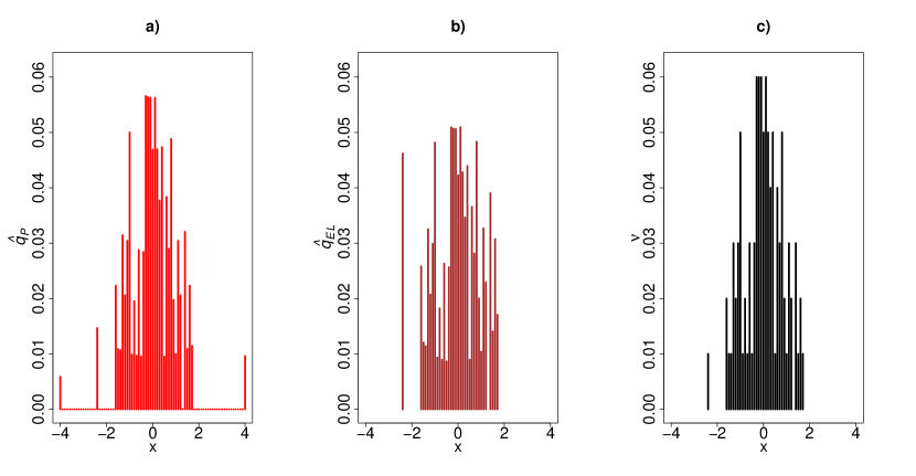
Figure 1: Panel a) the multinomial likelihood maximizing distribution $\hat{q}_{\scriptscriptstyle{\mathcal{P}}}$; panel b) the empirical likelihood maximizing distribution $\hat{q}_{\scriptscriptstyle{\mathcal{E}}}$; and panel c) the observed type $\nu$.

10 Implications for other methods

Besides the empirical likelihood, the minimum discrimination information, compositional data analysis, Lindsay geometry, bootstrap in the presence of auxiliary information, and Lagrange multiplier test ignore information about the alphabet, and are restricted to the observed data. Thus, they are affected by the above findings.

1) In the analysis of contingency tables with given marginals, the minimum discrimination information (MDI) method (cf. Ireland and Kullback [23]) is more popular than the maximum multinomial likelihood method. This is because the former is more computationally tractable, thanks to the generalized iterative scaling algorithm (cf. Ireland et al. [22]). MDI minimizes $I_{0}(q\,\|\,\nu)$ over $q$, so that a solution of the MDI problem must assign a zero mass to a passive, unobserved letter. Thus, MDI is effectively an empirical method. This implies that the MDI-minimizing distribution restricted to a convex closed set $C$ may not exist; however, the multinomial likelihood-maximizing distribution always exists (cf. Theorem 2), and may assign a positive mass to an unobserved outcome(s).

Example 30 (Contingency table with given marginals).

Consider a $3\times 3$ contingency table with given marginals. Let $\mathcal{X}=\{1,2,3\}\times\{1,2,3\}$, and let the observed bi-variate type $\nu$ have all the mass concentrated to $(1,1)$; the remaining eight possibilities have got zero counts. Let the column and raw marginals be $f_{c}=(1,2,7)/10$, $f_{r}=(5,4,1)/10$, respectively. One of the multinomial likelihood maximizing distributions $\hat{q}_{\scriptscriptstyle{\mathcal{P}}}$ is displayed in Table 2. In the active letter $\hat{q}^{a}_{\scriptscriptstyle{\mathcal{P}}}=0.1$ is unique, in the passive letters $\hat{q}^{p}_{\scriptscriptstyle{\mathcal{P}}}\in C^{p}(q^{a}_{\scriptscriptstyle{\mathcal{P}}})$. The table exhibits the $\hat{q}^{p}_{\scriptscriptstyle{\mathcal{P}}}$ which can also be obtained by the PP algorithm with the uniform activation (8.4). Note that $C^{a}(0^{p})=\emptyset$, so that the MDI-minimizing distribution does not exist.

$\hat{q}_{\scriptscriptstyle{\mathcal{P}}}$ 0.100 0.000 0.000 0.094 0.080 0.026 0.306 0.320 0.074

Table 2: A solution of $\mathcal{P}$.

It is worth stressing that the PP algorithm makes the multinomial likelihood primal problem $\mathcal{P}$ computationally feasible.

2) Multinomial likelihood maximization has the same solution regardless of whether the proportions $\nu$ or the counts $(n_{i})_{i\in\mathcal{X}}$ are used. Note that the vector $\nu$ of normalized frequencies is an instance of the compositional data. In the analysis of compositional data, it is assumed that the compositional data $(x_{1},\dots,x_{m})$ belong to $\{(x_{1},\dots,x_{m}):x_{1}>0,\dots,x_{m}>0,\sum x_{i}=1\}$; cf. Aitchison [3, Sect. 2.2]. This assumption transforms $\nu\in\Delta_{\mathcal{X}}$ into $\nu^{a}\in\Delta_{\mathcal{X}^{a}}$. Consequently, the multinomial likelihood problem $\mathcal{P}$ is replaced by the empirical likelihood problem $\mathcal{E}$. However, this replacement is not without consequences, as the solution of the empirical likelihood problem $\mathcal{E}$ (if it exists) may differ from the solution of $\mathcal{P}$; cf. Section 9.

3) Lindsay [28, Sect. 7.2] discusses multinomial mixtures under linear constraints on the mixture components, and assumes that it is sufficient to consider the distributions supported in the data (i.e., in the active alphabet). Though the objective function $\ell(\cdot)$ in $\mathcal{P}$ is a ‘single-component’ multinomial likelihood, the present results for the H-set, Z-set, and BD-gap suggest that it would be more appropriate to work with the complete alphabet; see also Anaya-Izquierdo et al. [5, Sect. 5.1].

4) Bootstrap in the presence of auxiliary information (cf. Zhang [45], Hall and Presnell [20]) in the form of a convex closed set, resamples from the EL-maximizing distribution $\hat{q}_{\scriptscriptstyle{\mathcal{E}}}$. Hence, this method intentionally discards information about the alphabet. Resampling from $\hat{q}_{\scriptscriptstyle{\mathcal{P}}}$ seems to be a better option.

5) The Lagrange multiplier (score) test (cf. Silvey [40]) of the linear restrictions on $q$ (cf. $C$ given by (2.3)) fails if $C$ is an H-set or a Z-set with respect to $\nu$, because the Lagrangean first-order conditions do not lead to a finite solution of $\mathcal{P}$. However, the multinomial likelihood ratio exists.

11 Proofs

11.1 Notation and preliminaries

In this section we introduce notation and recall notions and results which will be used later; it is based mainly on Bertsekas [9] and Rockafellar [38, 37]. We will not repeat the definitions introduced in the previous part of the paper.

We assume that the extended real line $\bar{\mathbb{R}}=[-\infty,\infty]$ is equipped with the order topology; so it is a compact metrizable space homeomorphic to the unit interval. The arithmetic operations on $\bar{\mathbb{R}}$ are defined in a usual way; further we put $0\cdot(\pm\infty)\triangleq 0$. For $\alpha\leq 0$ we define $\log(\alpha)\triangleq-\infty$; then $\log:\mathbb{R}\to\bar{\mathbb{R}}$ is continuous.

For $m\geq 0$ put $\mathbb{R}^{m}_{+}\triangleq\{x\in\mathbb{R}^{m}:x\geq 0\}$ and $\mathbb{R}^{m}_{-}\triangleq\{x\in\mathbb{R}^{m}:x\leq 0\}$ (recall that, for $m=0$, $\mathbb{R}^{m}=\{0\}$). In the matrix operations, the members of $\mathbb{R}^{m}$ are considered to be column matrices. If no confusion can arise, a vector with constant values is denoted by a scalar.

Let $C$ be a nonempty subset of $\mathbb{R}^{m}$. The convex hull of $C$ is denoted by $\operatorname{conv}(C)$. The polar cone of $C$ is the set $C^{\ast}\triangleq\{y\in\mathbb{R}^{m}:\ \left\langle y,q\right\rangle\leq 0\text{ for every }q\in C\}$. This is a nonempty closed convex cone [9, p. 166]. Assume that $C$ is convex. The relative interior $\operatorname{ri}(C)$ of $C$ is the interior of $C$ relative to the affine hull $\operatorname{aff}(C)$ of $C$ [9, p. 40]; it is nonempty and convex [9, Prop. 1.4.1].

The recession cone of a convex set $C$ is the convex cone

$$R_{C}\triangleq\{z\in\mathbb{R}^{m}:\ x+\alpha z\in C\text{ for every }x\in C,\alpha>0\}$$ (11.1)

[9, p. 50]. Every $z\in R_{C}$ is called a direction of recession of $C$. Clearly, $0\in R_{C}$; if $R_{C}=\{0\}$ it is said to be trivial. The lineality space $L_{C}$ of $C$ is defined by $L_{C}\triangleq R_{C}\cap(-R_{C})$ [9, p. 54]; it is a linear subspace of $\mathbb{R}^{m}$. Note that if $C$ is a cone then $R_{C}=C$ and $L_{C}=C\cap(-C)$.

Let $X$ be a subset of $\mathbb{R}^{m}$ and $f:X\to\bar{\mathbb{R}}$ be a function. By $f^{\prime}(x;y)$ we denote the directional derivative of $f$ at $x$ in the direction $y$ [9, p. 17]. By $\nabla f(x)$ and $\nabla^{2}f(x)$ we denote the gradient and the Hessian of $f$ at $x$. For a nonempty set $C\subseteq X$, $\operatorname*{argmin}_{C}{f}$ and $\operatorname*{argmax}_{C}{f}$ denote the sets of all minimizing and maximizing points of $f$ over $C$, respectively; that is,

$$\begin{split}&\operatorname*{argmin}_{C}{f}\,=\left\{\bar{x}\in C:\ f(\bar{x})=\inf_{x\in C}f(x)\right\},\qquad\\ &\operatorname*{argmax}_{C}{f}=\left\{\bar{x}\in C:\ f(\bar{x})=\sup_{x\in C}f(x)\right\}.\end{split}$$

The (effective) domain and the epigraph of $f$ are the sets [9, p. 25]

$$\operatorname{dom}(f)\triangleq\{x\in X:\ f(x)<\infty\}\quad\text{and}\quad\operatorname{epi}(f)\triangleq\{(x,w)\in X\times\mathbb{R}:f(x)\leq w\}.$$

A function $f:X\to\bar{\mathbb{R}}$ is

• proper if $f>-\infty$ and there is $x\in\mathbb{R}^{m}$ with $f(x)<\infty$ [9, p. 25] (this should not be confused with the properness associated with compactness of point preimages);

• closed if $\operatorname{epi}(f)$ is closed in $\mathbb{R}^{m+1}$ [9, p. 28];

• lower semicontinuous (lsc) if $f(x)\leq\liminf_{k}f(x_{k})$ for every $x\in X$ and every sequence $(x_{k})_{k}$ in $X$ converging to $x$ [9, p. 27]; analogously for the upper semicontinuity (usc);

• convex if both $X$ and $\operatorname{epi}(f)$ are convex [9, Def. 1.2.4];

• concave if $(-f)$ is convex.

When dealing with closedness of $f$, we will often use the following simple lemma [9, Prop. 1.2.2 and p. 28].

Lemma 31.

Let $f:X\to\bar{\mathbb{R}}$ be a map defined on a set $X\subseteq\mathbb{R}^{m}$. Define

$$\tilde{f}:\mathbb{R}^{m}\to\bar{\mathbb{R}},\qquad\tilde{f}(x)\triangleq\begin{cases}f(x)&\text{if }x\in X;\\ \infty&\text{if }x\not\in X.\end{cases}$$

Then the following are equivalent:

1. $f$ is closed;

2. $\tilde{f}$ is closed;

3. $\tilde{f}$ is lower semicontinuous;

4. the level sets $V_{\gamma}\triangleq\{x\in\mathbb{R}^{m}:\tilde{f}(x)\leq\gamma\}=\{x\in X:f(x)\leq\gamma\}$ are closed for every $\gamma\in\mathbb{R}$.

The recession cone $R_{f}$ of a proper convex closed function $f:\mathbb{R}^{m}\to\bar{\mathbb{R}}$ is the recession cone of any of its nonempty level sets $V_{\gamma}$ [9, p. 93]. The lineality space $L_{f}$ of $R_{f}$ is, due to the convexity of $f$, the set of directions $y$ in which $f$ is constant (that is, $f(x+\alpha y)=f(x)$ for every $x\in\operatorname{dom}(f)$ and $\alpha\in\mathbb{R}$); thus $L_{f}$ is also called the constancy space of $f$ [9, p. 97]. If $g:\mathbb{R}^{m}\to\bar{\mathbb{R}}$ is concave, the corresponding notions for $g$ are defined via the convex function $(-g)$.

The fundamental results underlying the importance of recession cones, are the following theorems ([9, Props. 2.3.2 and 2.3.4] or [38, Thm. 27.3]).

Theorem 32.

Let $C$ be a nonempty convex closed subset of $\mathbb{R}^{m}$ and $f:\mathbb{R}^{m}\to\bar{\mathbb{R}}$ be a proper convex closed function such that $C\cap\operatorname{dom}(f)\neq\emptyset$. Then the following are equivalent:

1. the set $\operatorname*{argmin}_{C}{f}$ of minimizing points of $f$ over $C$ is nonempty and compact;

2. $C$ and $f$ have no common nonzero direction of recession, that is,

   $$R_{C}\cap R_{f}=\{0\}.$$

Both conditions are satisfied, in particular, if $C\cap\operatorname{dom}(f)$ is bounded.

Theorem 33.

Let $C$ be a nonempty convex closed subset of $\mathbb{R}^{m}$ and $f:\mathbb{R}^{m}\to\bar{\mathbb{R}}$ be a convex closed function such that $C\cap\operatorname{dom}(f)\neq\emptyset$. If

$$R_{C}\cap R_{f}=L_{C}\cap L_{f},$$ (11.2)

or if

$$C\text{ is polyhedral}\qquad\text{and}\qquad R_{C}\cap R_{f}\subseteq L_{f},$$

then the set $\operatorname*{argmin}_{C}{f}$ of minimizing points of $f$ over $C$ is nonempty. Under condition (11.2), $\operatorname*{argmin}_{C}{f}$ can be written as $\tilde{C}+(L_{C}\cap L_{f})$, where $\tilde{C}$ is compact.

Standing Assumption.

If not stated otherwise, in the sequel it is assumed that a nonempty convex closed subset $C$ of $\Delta_{\mathcal{X}}$ having support $\mathcal{X}$, and a type $\nu\in\Delta_{\mathcal{X}}$ are given.

Since no confusion can arise, by $\ell$ we denote also an extension of the original function $\ell$ (defined in (2.1)) to $\mathbb{R}^{m}$ :

$$\ell:\mathbb{R}^{m}\to\bar{\mathbb{R}},\qquad\ell(x)\triangleq-\left\langle\nu,\log(x)\right\rangle=-\sum_{i\in\mathcal{X}^{a}}\nu_{i}^{a}\log(x_{i}^{a});$$ (11.3)

the conventions $0\cdot(-\infty)=0$ and $\log\beta=-\infty$ for every $\beta\leq 0$ apply.

11.2 Proof of Theorem 2 (Primal problem)

In the next lemma we prove that $\ell$ is a proper convex closed function. Since $C$ is compact, $C$ has no nonzero direction of recession. From this and Theorem 32, Theorem 2 will follow.

Lemma 34.

If $\nu\in\Delta_{\mathcal{X}}$ and $\ell$ is given by (11.3), then

1. $\ell(x)>-\infty$ for every $x\in\mathbb{R}^{m}$, and $\ell(x)<\infty$ if and only if $x^{a}>0$; so

   $$\operatorname{dom}(\ell)=\{x\in\mathbb{R}^{m}:\ x^{a}>0\};$$

2. $\ell$ is a proper continuous (hence closed) convex function;

3. the restriction of $\ell$ to its domain ${\operatorname{dom}(\ell)}$ is strictly convex if and only if $\nu>0$;

4. $\ell$ is differentiable on $\operatorname{dom}(\ell)$ with the gradient given by

   $$\nabla\ell(x)=-(\nu^{a}/x^{a},0^{p});$$

   the one-sided directional derivative of $\ell$ at $x\in\operatorname{dom}(\ell)$ in the direction $y$ is

   $$\ell^{\prime}(x;y)=\left\langle\nabla\ell(x),y\right\rangle=-\sum_{i\in\mathcal{X}^{a}}\frac{\nu_{i}^{a}y_{i}^{a}}{x_{i}^{a}}\,;$$

5. the recession cone $R_{\ell}$ and the constancy space $L_{\ell}$ of $\ell$ are

   $$R_{\ell}=\{z\in\mathbb{R}^{m}:\ z^{a}\geq 0\}\quad\text{and}\quad L_{\ell}=\{z\in\mathbb{R}^{m}:\ z^{a}=0\}.$$

Proof.

The properties (a) and (d) are trivial and the property (b) follows from the continuity and concavity of the logarithm (extended to the whole real line); closedness of $\ell$ follows from continuity by Lemma 31. For the property (c), use that the Hessian $\nabla^{2}\ell(x)=(\partial^{2}\ell(x)/\partial x_{i}\partial x_{j})_{ij}$ is a diagonal matrix $\operatorname{diag}(\nu^{a}/(x^{a})^{2},0^{p})$. Hence it is positive definite and $\ell$ is strictly convex if and only if $\nu>0$ [9, Prop. 1.2.6].

It remains to prove (e). Fix any $\gamma\in\mathbb{R}$ such that the level set $V=\{x:\ \ell(x)\leq\gamma\}$ is nonempty. If $z$ is such that $z^{a}\not\geq 0$ then there is an active letter $i$ with $z_{i}<0$. In such a case, for any $x\in V$ there is $\alpha>0$ with $y_{i}+\alpha z_{i}\leq 0$ and so $y+\alpha z\not\in\operatorname{dom}(\ell)\supseteq V$. Hence, by (11.1), $z\not\in R_{V}=R_{\ell}$.

Now take any $z$ with $z^{a}\geq 0$. Then, for every $x\in V$ and $\alpha>0$, $\ell(x+\alpha z)\leq\ell(x)$ by the monotonicity of the logarithm. That is, $x+\alpha z\in V$ and so $z\in R_{V}=R_{\ell}$. The property (e) is proved. ∎

Proposition 35.

If the support of $C$ is $\mathcal{X}$, then the primal $\mathcal{P}$ is finite and its solution set $S_{\scriptscriptstyle{\mathcal{P}}}$ is nonempty and compact. Moreover, if $\nu>0$ then $S_{\scriptscriptstyle{\mathcal{P}}}$ is a singleton.

Proof.

Since $C$ is compact, its recession cone is trivial. Thus the first assertion follows from Theorem 32. The fact that $S_{\scriptscriptstyle{\mathcal{P}}}$ is a singleton provided $\nu>0$, follows from the strict convexness of $f$. ∎

Proposition 36.

Let $\nu\in\Delta_{\mathcal{X}}$ and $C$ be a convex closed set having support $\mathcal{X}$. Then the $\pi^{a}$-projection of $S_{\scriptscriptstyle{\mathcal{P}}}$ onto active letters is always a singleton $\{\hat{q}_{\scriptscriptstyle{\mathcal{P}}}^{a}\}$ and

$$S_{\scriptscriptstyle{\mathcal{P}}}=\{q\in C:\ q^{a}=\hat{q}^{a}_{\scriptscriptstyle{\mathcal{P}}}\}=\{\hat{q}^{a}_{\scriptscriptstyle{\mathcal{P}}}\}\times C^{p}(\hat{q}^{a}_{\scriptscriptstyle{\mathcal{P}}}).$$

Consequently, $S_{\scriptscriptstyle{\mathcal{P}}}$ is a singleton if and only if $C^{p}(\hat{q}^{a}_{\scriptscriptstyle{\mathcal{P}}})$ is a singleton.

Proof.

Note that $C^{a}=\pi^{a}(C)$ is a nonempty convex closed subset of $\mathbb{R}^{m_{a}}$. Define $\ell^{a}:\mathbb{R}^{m_{a}}\to\bar{\mathbb{R}}$ by $\ell^{a}(x^{a})\triangleq-\left\langle\nu^{a},\log x^{a}\right\rangle$ for $x^{a}\in C^{a}$ and $\ell^{a}(x^{a})\triangleq\infty$ otherwise. Since

$$\ell(q)=\ell^{a}(q^{a})\qquad\text{for every}\quad q\in C,$$ (11.4)

it holds that

$$\inf_{x^{a}\in C^{a}}\ell^{a}(x^{a})=\hat{\ell}_{\scriptscriptstyle{\mathcal{P}}}.$$

The map $\ell^{a}$ is proper, convex and closed (use Lemma 31 and the fact that the restriction of $\ell^{a}$ to the closed set ${C^{a}}$ is continuous, hence closed). Since $\operatorname{dom}(\ell^{a})\subseteq C^{a}$ is bounded, Theorem 32 gives that $\operatorname*{argmin}\ell^{a}$ is a nonempty compact set. This set is a subset of $\operatorname{dom}(\ell^{a})$ and the restriction of $\ell^{a}$ to $\operatorname{dom}(\ell^{a})$ is strictly convex (Lemma 34(c)), so $\operatorname*{argmin}\ell^{a}$ is a singleton. Hence there is a unique point $\hat{q}^{a}_{\scriptscriptstyle{\mathcal{P}}}\in C^{a}$ such that $\ell^{a}(\hat{q}^{a}_{\scriptscriptstyle{\mathcal{P}}})=\hat{\ell}_{\scriptscriptstyle{\mathcal{P}}}$. Now, (11.4) gives that $q\in S_{\scriptscriptstyle{\mathcal{P}}}$ if and only if $q^{a}=\hat{q}^{a}_{\scriptscriptstyle{\mathcal{P}}}$; so $S_{\scriptscriptstyle{\mathcal{P}}}=\{\hat{q}^{a}_{\scriptscriptstyle{\mathcal{P}}}\}\times C^{p}(\hat{q}^{a}_{\scriptscriptstyle{\mathcal{P}}})$. ∎

Theorem 2 immediately follows from Propositions 35 and 36.

11.3 Proof of Theorem 5 (Convex conjugate by Lagrange duality)

In this section we prove Theorem 5 on the convex conjugate $\ell^{\ast}$, defined by the convex conjugate primal problem (cc-primal, for short)

$$\ell^{\ast}(z)=\sup_{q\in\Delta_{\mathcal{X}}}(\left\langle q,z\right\rangle-\ell(q)).$$

The proof is based on the following reformulation of the cc-primal

$$\ell^{\ast}(z)=\adjustlimits{\sup}_{x\geq 0}{\inf}_{\mu\in\mathbb{R}}K_{z}(x,\mu)=\adjustlimits{\inf}_{\mu\in\mathbb{R}}{\sup}_{x\geq 0}K_{z}(x,\mu),$$

where

$$K_{z}(x,\mu)=\left\langle x,z\right\rangle+\left\langle\nu,\log x\right\rangle-\mu\left(\sum x-1\right)$$

is the Lagrangian function; cf. Lemma 38. Then we will show that the map $\mu\mapsto\sup_{x\geq 0}K_{z}(x,\mu)$ is minimized at $\hat{\mu}(z)=\max\{\bar{\mu}(z^{a}),\max(z^{p})\}$; cf. Section 11.3.2. Structure of the solution set $S_{cc}(z)$ of the cc-primal is described in Section 11.3.3. Additional properties of the convex conjugate, which will be utilized in the proof of Theorem 6, are stated in Section 11.3.4.

For every $z^{a}\in\mathbb{R}^{m_{a}}$ and $\mu>\max(z^{a})$ put

$$\xi(\mu)=\xi_{z^{a}}(\mu)\triangleq\sum\frac{\nu^{a}}{\mu-z^{a}}$$ (11.5)

and recall that $\hat{\mu}(z)\triangleq\max\{\bar{\mu}(z^{a}),\max(z^{p})\}$, where $\bar{\mu}(z^{a})>\max(z^{a})$ solves $\xi(\mu)=1$. Since

$$\xi\text{ is strictly decreasing},\quad\lim_{\mu\searrow\max(z^{a})}\xi(\mu)=\infty\quad\text{and}\quad\lim_{\mu\to\infty}\xi(\mu)=0,$$ (11.6)

$\bar{\mu}(z^{a})$ is well-defined. We start with a simple lemma.

Lemma 37.

For every $z\in\mathbb{R}^{m}$ and $c\in\mathbb{R}$,

$$\bar{\mu}(z^{a}+c)=\bar{\mu}(z^{a})+c,\quad\hat{\mu}(z+c)=\hat{\mu}(z)+c,\quad\text{and}\quad\ell^{\ast}(z+c)=\ell^{\ast}(z)+c.$$

Proof.

The first two equalities follow from the facts that $\xi_{z^{a}+c}(\cdot+c)=\xi_{z^{a}}(\cdot)$ and that $\max(z^{p}+c)=\max(z^{p})+c$. The final one is a trivial consequence of the definition of $\ell^{\ast}$; indeed, since $\left\langle q,c\right\rangle=c$ for every $q\in\Delta_{\mathcal{X}}$, $\ell^{\ast}(z+c)=\sup_{q}(\left\langle q,(z+c)\right\rangle-\ell(q))=\ell^{\ast}(z)+c$. ∎

11.3.1 Lagrange duality for the convex conjugate

Assume that $\nu\in\Delta_{\mathcal{X}}$ and $z\in\mathbb{R}^{m}$ are given. For $x\in\mathbb{R}^{m}_{+}$ put

$$h_{z}(x)\triangleq\left\langle x,z\right\rangle-\ell(x)=\left\langle x,z\right\rangle+\left\langle\nu^{a},\log x^{a}\right\rangle$$

and define extended-real-valued functions

$$K_{z}:\mathbb{R}^{m}\times\mathbb{R}\to\bar{\mathbb{R}},\quad K_{z}(x,\mu) \triangleq\begin{cases}h_{z}(x)-\mu\left(\sum x-1\right)&\text{if }x\in\mathbb{R}^{m}_{+},\mu\in\mathbb{R},\\ \infty&\text{otherwise};\end{cases}$$

$$k_{z}:\mathbb{R}\to\bar{\mathbb{R}},\quad\qquad\quad k_{z}(\mu) \triangleq\sup_{x\in\mathbb{R}^{m}_{+}}K_{z}(x,\mu).$$

Lemma 38 (Lagrange duality for the convex conjugate).

For every $\nu\in\Delta_{\mathcal{X}}$ and $z\in\mathbb{R}^{m}$,

$$\ell^{\ast}(z)=\inf_{\mu\in\mathbb{R}}k_{z}(\mu)=\adjustlimits{\inf}_{\mu\in\mathbb{R}}{\sup}_{x\geq 0}K_{z}(x,\mu).$$

Proof.

We follow [37, Sect. 4]. Denote by $\mathbb{R}^{m}_{\oplus}$ the subset $\{x\in\mathbb{R}^{m}:x^{a}>0,x^{p}\geq 0\}$ of $\mathbb{R}^{m}_{+}$. Define $F_{z}:\mathbb{R}^{m}\times\mathbb{R}^{2}\to\bar{\mathbb{R}}$ and $f_{z}:\mathbb{R}^{m}\to\bar{\mathbb{R}}$ by

$$F_{z}(x,u) \triangleq \begin{cases}-h_{z}(x)&\text{if }x\in\mathbb{R}^{m}_{\oplus},1-u_{2}\leq\sum x\leq 1+u_{1};\\ \infty&\text{otherwise};\end{cases}$$

$$f_{z}(x) \triangleq F_{z}(x,0).$$

Note that, in the definition of $F_{z}$, $x\in\mathbb{R}^{m}_{\oplus}$ can be replaced by $x\in\mathbb{R}^{m}_{+}$; indeed, if $x\in\mathbb{R}^{m}_{+}\setminus\mathbb{R}^{m}_{\oplus}$ then $x_{i}^{a}=0$ for some $i\in\mathcal{X}^{a}$ and hence $-h_{z}(x)=\infty$. The set $D\triangleq\{(x,u)\in\mathbb{R}^{m}\times\mathbb{R}^{2}:x\geq 0,1-u_{2}\leq\sum x\leq 1+u_{1}\}$ is closed convex (in fact, polyhedral) and the map $\tilde{F}_{z}:D\to\bar{\mathbb{R}}$, $(x,u)\mapsto-h_{z}(x)$ is convex and continuous, hence closed. Since the epigraphs of $\tilde{F}_{z}$ and $F_{z}$ coincide,

$$F_{z}\quad\text{is convex and closed jointly in }x\text{ and }u.$$ (11.7)

The corresponding optimal value function $\varphi_{z}:\mathbb{R}^{2}\to\bar{\mathbb{R}}$ is defined by (cf. [37, (4.7)])

$$\varphi_{z}(u)\triangleq\inf_{x\in\mathbb{R}^{m}}F_{z}(x,u).$$

We are going to show that

$$\varphi_{z}(0)=\liminf_{u\to 0}\varphi_{z}(u).$$ (11.8)

To this end, take any $\varepsilon\in(0,1)$ and $u\in\mathbb{R}^{2}$ with $\lvert u\rvert<1$. Assume that $u_{1}+u_{2}\geq 0$. Then

$$\varphi_{z}(u)=\inf_{\begin{subarray}{c}x\geq 0\\ \sum x\in[1-u_{2},1+u_{1}]\end{subarray}}(-h_{z}(x))=\inf_{\theta\in[1-u_{2},1+u_{1}]}\ \inf_{x\in\Delta_{\mathcal{X}}}(-h_{z}(\theta x)).$$

For any $\theta>0$,

$$\begin{split}\sup_{x\in\Delta_{\mathcal{X}}}\lvert h_{z}(\theta x)-h_{z}(x)\rvert&\leq\sup_{x\in\Delta_{\mathcal{X}}}\left(\lvert\log\theta\rvert+\lvert 1-\theta\rvert\cdot\lvert\left\langle x,z\right\rangle\rvert\right)\\ &=\lvert\log\theta\rvert+\lvert 1-\theta\rvert\cdot\max\lvert z\rvert\triangleq\psi_{z}(\theta).\end{split}$$

Since $\psi_{z}$ is continuous at $\theta=1$ and $\psi_{z}(1)=0$, there is $\delta>0$ such that $\psi_{z}(\theta)<\varepsilon$ for every $\theta\in[1-\delta,1+\delta]$. Thus $\lvert\varphi_{z}(u)-\varphi_{z}(0)\rvert<\varepsilon$ whenever $\lvert u\rvert<\delta$ and $u_{1}+u_{2}\geq 0$. This gives

$$\varphi_{z}(0)=\lim_{\begin{subarray}{c}u\to 0\\ u_{1}+u_{2}\geq 0\end{subarray}}\varphi_{z}(u).$$

Since $\varphi_{z}(u)=\infty$ if $u_{1}+u_{2}<0$ (indeed, for such $u$, $F_{z}(x,u)=\infty$ for every $x$), (11.8) is proved.

The Lagrangian function $L_{z}:\mathbb{R}^{m}\times\mathbb{R}^{2}\to\bar{\mathbb{R}}$ associated with $F_{z}$ is defined by (cf. [37, (4.2)])

$$L_{z}(x,y)\triangleq\inf_{u\in\mathbb{R}^{2}}\left(F_{z}(x,u)+\left\langle u,y\right\rangle\right).$$

A simple computation yields (cf. [37, (4.4)] with $f_{0}(x)=h_{z}(x)$, $f_{1}(x)=\sum x-1$, and $f_{2}(x)=1-\sum x$, all restricted to $C=\mathbb{R}^{m}_{\oplus}$)

$$L_{z}(x,y)=\begin{cases}-h_{z}(x)+(y_{1}-y_{2})\left(\sum x-1\right)&\text{if }x\in\mathbb{R}^{m}_{\oplus},y\in\mathbb{R}^{2}_{+};\\ -\infty&\text{if }x\in\mathbb{R}^{m}_{\oplus},y\not\in\mathbb{R}^{2}_{+};\\ \infty&\text{if }x\not\in\mathbb{R}^{m}_{\oplus}.\end{cases}$$

(Indeed, fix any $x\in\mathbb{R}^{m}$ and $y\in\mathbb{R}^{2}$. If $x\not\in\mathbb{R}^{m}_{\oplus}$ then $F_{z}(x,u)=\infty$ for every $u$, hence $L_{z}(x,y)=\infty$. If $x\in\mathbb{R}^{m}_{\oplus}$ and $y\not\geq 0$, then $F_{z}(x,u)=-h_{z}(x)$ whenever both $u_{1},u_{2}>0$ are sufficiently large; for such $u$, $\left\langle u,y\right\rangle$ is not bounded from below (use that $y_{1}<0$ or $y_{2}<0$), hence $L_{z}(x,y)=-\infty$. Finally, assume that $x\in\mathbb{R}^{m}_{\oplus}$ and $y\geq 0$. If $u_{1}+u_{2}<0$ then $F_{z}(x,u)=\infty$ by the definition of $F_{z}$. If $u_{1}+u_{2}\geq 0$ then $\left\langle u,y\right\rangle\geq y_{1}(\sum x-1)+y_{2}(1-\sum x)$, with the equality if $u_{1}=\sum x-1$, $u_{2}=1-\sum x$. Thus $L_{z}(x,y)=-h_{z}(x)+(y_{1}-y_{2})\left(\sum x-1\right)$.)

If we define (cf. [37, (4.6)])

$$g_{z}:\mathbb{R}^{2}\to\bar{\mathbb{R}},\qquad g_{z}(y)\triangleq\inf_{x\in\mathbb{R}^{m}}L_{z}(x,y),$$

then [37, Thm. 7], (11.7), and (11.8) imply

$$\inf_{x\in\mathbb{R}^{m}}f_{z}(x)=\varphi_{z}(0)=\liminf_{u\to 0}\varphi_{z}(u)=\sup_{y\in\mathbb{R}^{2}}g_{z}(y).$$

By the definition of $f_{z}$, $\inf_{x}f_{z}(x)=-\ell^{\ast}(z)$; thus to finish the proof of the lemma it suffices to show that

$$\inf_{\mu\in\mathbb{R}}k_{z}(\mu)=-\sup_{y\in\mathbb{R}^{2}}g_{z}(y).$$ (11.9)

If $y\not\in\mathbb{R}^{2}_{+}$ then $g_{z}(y)=-\infty$; to see this, take arbitrary $x\in\mathbb{R}^{m}_{\oplus}$ and realize that $g_{z}(y)\leq L_{z}(x,y)=-\infty$. Fix any $y\in\mathbb{R}^{2}_{+}$. Then, for every $x\in\mathbb{R}^{m}_{\oplus}$, $K_{z}(x,y_{1}-y_{2})=-L_{z}(x,y)$; hence

$$k_{z}(y_{1}-y_{2})=-g_{z}(y).$$

Since $\{y_{1}-y_{2}:y\in\mathbb{R}^{2}_{+}\}=\mathbb{R}$, we have

$$\inf_{\mu\in\mathbb{R}}k_{z}(\mu)=\inf_{y\in\mathbb{R}^{2}_{+}}(-g_{z}(y))=-\sup_{y\in\mathbb{R}^{2}}g_{z}(y).$$

Thus (11.9) is established and the proof of the lemma is finished. ∎

11.3.2 Proof of Theorem 5

With Lemma 38, Theorem 5 can be proved. Recall that the theorem states that, for every $z\in\mathbb{R}^{m}$,

$$\ell^{\ast}(z)=-1+\hat{\mu}(z)+I_{\hat{\mu}(z)}(\nu^{a}\,\|\,-z^{a}),\qquad\text{where}\quad\hat{\mu}(z)\triangleq\max\{\bar{\mu}(z^{a}),\max(z^{p})\}.$$

Proof of Theorem 5.

Keep the notation from Section 11.3.1. By Lemma 38, $\ell^{\ast}(z)=\inf_{\mu\in\mathbb{R}}k_{z}(\mu)$, and, using partial maximization,

$$k_{z}(\mu)=\sup_{x^{a}\geq 0}\tilde{k}_{z}(x^{a},\mu),\quad\text{where}\quad\tilde{k}_{z}(x^{a},\mu)\triangleq\sup_{x^{p}\geq 0}{K}_{z}((x^{a},x^{p}),\mu).$$

Note that $K_{z}(x,\mu)=c+\sum_{i\in\mathcal{X}^{p}}x_{i}^{p}(z_{i}^{p}-\mu)$, where $c$ does not depend on $x^{p}$. Thus

$$\tilde{k}_{z}(x^{a},\mu)=\begin{cases}\left\langle x^{a},z^{a}\right\rangle+\left\langle\nu^{a},\log x^{a}\right\rangle-\mu\left(\sum x^{a}-1\right)&\text{if }\mu\geq\max(z^{p});\\ \infty&\text{otherwise}.\end{cases}$$ (11.10)

The second case immediately gives

$$k_{z}(\mu)=\infty\qquad\text{if}\quad\mu<\max(z^{p}).$$ (11.11)

If $\mu\geq\max(z^{p})$ and $z_{i}^{a}-\mu\geq 0$ for some $i\in\mathcal{X}^{a}$, then $k_{z}(\mu)=\infty$ (use (11.10) and the fact that, for any $a\geq 0$ and $b>0$, the map $f(x)\triangleq ax+b\log x$ is strictly increasing and $\lim_{x\to\infty}f(x)=\infty$). That is

$$k_{z}(\mu)=\infty\qquad\text{if}\quad\mu\leq\max(z^{a}).$$ (11.12)

Assume now that $\mu\geq\max(z^{p})$ and $\mu>\max(z^{a})$. Note that

$$k_{z}(\mu)=\max_{x^{a}>0}\tilde{k}_{z}(x^{a},\mu).$$

By (11.10), $\tilde{k}_{z}(\cdot,\mu)$ is differentiable and strictly concave on the open set $\{x^{a}\in\mathbb{R}^{m_{a}}:x^{a}>0\}$ (use that the Hessian, which is equal to $\operatorname{diag}(-\nu_{i}^{a}/(x_{i}^{a})^{2})_{i=1}^{m_{a}}$, is negative definite). Thus the basic necessary and sufficient condition for unconstrained optimization [9, p. 258] gives that

$$k_{z}(\mu)=\tilde{k}_{z}(\hat{x}^{a},\mu),$$

where $\hat{x}^{a}=\hat{x}^{a}_{\mu}>0$ is the unique solution of $\nabla_{x^{a}}\tilde{k}_{z}(\hat{x}^{a},\mu)=0$; that is,

$$z_{i}^{a}+\frac{\nu_{i}^{a}}{\hat{x}_{i}^{a}}-\mu=0\qquad\text{for every}\quad i\in\mathcal{X}^{a}.$$

The above equation immediately yields

$$\hat{x}^{a}=\frac{\nu^{a}}{\mu-z^{a}}$$

and

$$k_{z}(\mu)=-1+\mu+I_{\mu}(\nu^{a}\,\|\,-z^{a})\qquad\text{if}\quad\mu\geq\max(z^{p}),\mu>\max(z^{a}).$$ (11.13)

Put $J\triangleq\{\mu\in\mathbb{R}:\mu>\max(z^{a}),\mu\geq\max(z^{p})\}$ and $\underline{\mu}\triangleq\max(z)$; then either $J=(\underline{\mu},\infty)$ or $J=[\underline{\mu},\infty)$. Equations (11.11), (11.12), and (11.13) yield

$$k_{z}(\mu)=\begin{cases}-1+\mu+I_{\mu}(\nu^{a}\,\|\,-z^{a})&\text{if }\mu\in J;\\ \infty&\text{otherwise}.\end{cases}$$

For $\mu>\underline{\mu}$ we have

$$k_{z}^{\prime}(\mu)=1-\xi(\mu).$$

Since $\xi$ is decreasing on $J$ and $\xi(\bar{\mu}(z^{a}))=1$, $k_{z}(\mu)$ is decreasing on $[\underline{\mu},\bar{\mu}(z^{a})]$ and increasing on $[\bar{\mu}(z^{a}),\infty)$, provided $\underline{\mu}\leq\bar{\mu}(z^{a})$; otherwise $k_{z}(\mu)$ is increasing on $[\underline{\mu},\infty]$. Thus,

$$\ell^{\ast}(z)=\inf_{\mu\in\mathbb{R}}k_{z}(\mu)=\begin{cases}k_{z}(\bar{\mu}(z^{a}))&\text{if }\bar{\mu}(z^{a})\geq\underline{\mu};\\ k_{z}(\underline{\mu})&\text{otherwise}.\end{cases}$$

So $\operatorname*{argmin}k_{z}=\max\{\bar{\mu}(z^{a}),\max(z^{p})\}=\hat{\mu}(z)$ and Theorem 5 is proved. ∎

Corollary 39.

If $\nu>0$ then, for every $z\in\mathbb{R}^{m}$,

$$\begin{split}\ell^{\ast}(z)&=-1+\bar{\mu}(z)+I_{\bar{\mu}(z)}(\nu\,\|\,-z)\\ &=-1+\bar{\mu}(z)+\left\langle\nu,\log\nu\right\rangle-\left\langle\nu,\log(\bar{\mu}(z)-z)\right\rangle.\end{split}$$

Corollary 39 was first proved by El Barmi and Dykstra [10, Lemma 2.1].

11.3.3 The structure of the solution set $S_{cc}(z)$

The structure of the cc-primal solution set $S_{cc}(z)$, defined by (3.2), is described. First, recall the definition (11.5) of $\xi$.

Proposition 40.

For every $z\in\mathbb{R}^{m}$, $S_{cc}(z)$ is a nonempty compact set and

$$\begin{split}S_{cc}(z)=\{\hat{q}^{a}_{cc}(z)\}\times\{&q^{p}\geq 0:\sum q^{p}=1-\xi(\hat{\mu}(z)),\\ &q^{p}_{i}=0\text{ whenever }z^{p}_{i}\neq\hat{\mu}(z)\},\end{split}$$

where

$$\hat{q}^{a}_{cc}(z)\triangleq\frac{\nu^{a}}{\hat{\mu}(z)-z^{a}}.$$

In particular, if $\bar{\mu}(z^{a})\geq\max(z^{p})$ then $S_{cc}(z)=\{(\hat{q}^{a}_{cc}(z),0^{p})\}$ is a singleton.

Proof.

Fix $z\in\mathbb{R}^{m}$ and put $\mu\triangleq\hat{\mu}(z)$, $\hat{q}^{a}_{cc}\triangleq\hat{q}^{a}_{cc}(z)$; then, by Theorem 5, $\ell^{\ast}(z)=-1+\mu+I_{\mu}(\nu^{a}\,\|\,-z^{a})$. The fact that $S_{cc}(z)$ is nonempty and compact follows from Theorem 32.

Take any $\bar{q}\in S_{cc}(z)$. Then $\bar{q}^{a}>0$ and, for every $q\in\Delta_{\mathcal{X}}$,

$$0\geq f_{z}^{\prime}(\bar{q};q-\bar{q})=\left\langle z,(q-\bar{q})\right\rangle+\sum\frac{\nu^{a}q^{a}}{\bar{q}^{a}}-1.$$

If also $q\in S_{cc}(z)$ then, analogously,

$$0\geq\left\langle z,(\bar{q}-q)\right\rangle+\sum\frac{\nu^{a}\bar{q}^{a}}{q^{a}}-1.$$

Thus, by combining these two inequalities,

$$\sum\nu^{a}\left(\frac{q^{a}}{\bar{q}^{a}}+\frac{\bar{q}^{a}}{q^{a}}\right)\leq 2.$$

For positive $x$ and $y$, $(x/y+y/x)\geq 2$, with equality if and only if $x=y$. Thus, $q^{a}=\bar{q}^{a}$ for every $\bar{q},q\in S_{cc}(z)$; hence,

$$\pi^{a}(S_{cc}^{a}(z))\quad\text{is a singleton}.$$ (11.14)

Distinguish two cases. First assume that $\mu=\bar{\mu}(z^{a})\geq\max(z^{p})$ and put $\bar{q}\triangleq(\hat{q}^{a}_{cc},0^{p})$. Then $\bar{q}\in\Delta_{\mathcal{X}}$ (use that $\sum\bar{q}=\xi(\mu)=1$) and

$$f_{z}(\bar{q}) = \left\langle\hat{q}^{a}_{cc},z^{a}\right\rangle+\left\langle\nu^{a},\log(\hat{q}^{a}_{cc})\right\rangle=\sum\frac{(z^{a}-\mu+\mu)\nu^{a}}{\mu-z^{a}}+I_{\mu}(\nu^{a}\,\|\,-z^{a})$$

$$= -1+\mu+I_{\mu}(\nu^{a}\,\|\,-z^{a})=\ell^{\ast}(z).$$

Hence $\bar{q}\in S_{cc}(z)$ and, since $\sum\bar{q}^{a}=1$, $S_{cc}(z)=\{\bar{q}\}$ by (11.14).

Assume now that $\mu=\max(z^{p})>\bar{\mu}(z^{a})$; then $\gamma\triangleq\xi(\mu)<\xi(\bar{\mu}(z^{a}))=1$. Take any $\bar{q}\in\Delta_{\mathcal{X}}$ with $\bar{q}^{a}=\hat{q}^{a}_{cc}$ and note that $\sum\bar{q}^{p}=1-\gamma$. An argument analogous to the first case gives

$$f_{z}(\bar{q})=\left\langle\bar{q}^{p},z^{p}\right\rangle+\left\langle\hat{q}^{a},z^{a}\right\rangle+\left\langle\nu^{a},\log(\hat{q}^{a}_{cc})\right\rangle=\left\langle\bar{q}^{p},z^{p}\right\rangle-1+\mu\gamma+I_{\mu}(\nu^{a}\,\|\,-z^{a}).$$

Hence $\bar{q}\in S_{cc}(z)$ if and only if $\left\langle\bar{q}^{p},z^{p}\right\rangle=\mu(1-\gamma)$. Since $\sum\bar{q}^{p}=1-\gamma$, the last condition is equivalent to the fact that $\bar{q}^{p}_{i}=0$ for every $i\in\mathcal{X}^{p}$ with $z^{p}_{i}<\mu$. In view of (11.14) this proves the proposition. ∎

11.3.4 Additional properties of the convex conjugate

Some additional properties of the convex conjugate $\ell^{\ast}$, concerning its monotonicity and differentiability, are summarized in the next lemmas.

Lemma 41.

The following is true for every $z,\tilde{z}\in\mathbb{R}^{m}$:

1. If $z^{a}\geq\tilde{z}^{a}$ then $\bar{\mu}(z^{a})\geq\bar{\mu}(\tilde{z}^{a})$, with the equality if and only if $z^{a}=\tilde{z}^{a}$.

2. If $z\geq\tilde{z}$ then $\ell^{\ast}(z)\geq\ell^{\ast}(\tilde{z})$ (that is, $\ell^{\ast}$ is nondecreasing), with the equality if and only if $z^{a}=\tilde{z}^{a}$ and $\hat{\mu}(z)=\hat{\mu}(\tilde{z})$.

Proof.

(a) If $z^{a}\geq\tilde{z}^{a}$ then $\xi_{z^{a}}(\mu)\geq\xi_{\tilde{z}^{a}}(\mu)$ for every $\mu>\max(z^{a})$; moreover, $\xi_{z^{a}}(\mu)=\xi_{\tilde{z}^{a}}(\mu)$ for some $\mu>\max(z^{a})$ if and only if $z^{a}=\tilde{z}^{a}$. Using (11.6), (a) follows.

(b) Assume that $z\geq\tilde{z}$. Then $\left\langle z,q\right\rangle\geq\left\langle\tilde{z},q\right\rangle$ for every $q\in\Delta_{\mathcal{X}}$, hence $\ell^{\ast}(z)\geq\ell^{\ast}(\tilde{z})$. If $z^{a}=\tilde{z}^{a}$ and $\hat{\mu}(z)=\hat{\mu}(\tilde{z})$ then $\ell^{\ast}(z)=\ell^{\ast}(\tilde{z})$ by Theorem 5. It suffices to prove that if $z^{a}\neq\tilde{z}^{a}$ or $\hat{\mu}(z)\neq\hat{\mu}(\tilde{z})$ then $\ell^{\ast}(z)>\ell^{\ast}(\tilde{z})$.

To this end, fix some $\tilde{q}\in S_{cc}(\tilde{z})$. If $z^{a}\neq\tilde{z}^{a}$ then $\ell^{\ast}(z)\geq\left\langle\tilde{q},z\right\rangle-\ell(\tilde{q})\geq\left\langle\tilde{q}^{a},(z^{a}-\tilde{z}^{a})\right\rangle+\ell^{\ast}(\tilde{z})$. Since $\tilde{q}^{a}>0$ and $(z^{a}-\tilde{z}^{a})\geq 0$ is not zero, we have $\ell^{\ast}(z)>\ell^{\ast}(\tilde{z})$. Finally, assume that $z^{a}=\tilde{z}^{a}$ and $\hat{\mu}(z)>\hat{\mu}(\tilde{z})$. The map

$$g:[\bar{\mu}({z}^{a}),\infty)\to\mathbb{R},\qquad g(\mu)\triangleq\mu+I_{\mu}(\nu^{a}\,\|\,-z^{a})$$

is strictly increasing (indeed, $g^{\prime}(\mu)=1-\xi(\mu)>0$ for $\mu>\bar{\mu}({z}^{a})$ by (11.6)). Thus, by Theorem 5 and the fact that $\hat{\mu}(\tilde{z})\geq\bar{\mu}(\tilde{z}^{a})=\bar{\mu}(z^{a})$, it follows that $\ell^{\ast}(z)-\ell^{\ast}(\tilde{z})=g(\hat{\mu}(z))-g(\hat{\mu}(\tilde{z}))>0$. ∎

Since the convex conjugate $\ell^{\ast}$ is finite-valued and convex, by [38, Thm. 10.4] it is locally Lipschitz. The following lemma claims that $\ell^{\ast}$ is even globally Lipschitz with the Lipschitz constant equal to $1$. (Here we assume that $\mathbb{R}^{m}$ is equipped with the sup-norm $\|x\|_{\infty}=\max\lvert x_{i}\rvert$.)

Lemma 42.

The convex conjugate $\ell^{\ast}:\mathbb{R}^{m}\to\mathbb{R}$ is a (finite-valued) convex function which is Lipschitz with $\operatorname{Lip}(\ell^{\ast})=1$.

Proof.

The fact that $\ell^{\ast}$ is always finite is obvious. To prove that $\ell^{\ast}$ is Lipschitz-$1$, fix any $z,z^{\prime}\in\mathbb{R}^{m}$. Then, for any $q\in S_{cc}(z)$,

$$\ell^{\ast}(z)-\ell^{\ast}(z^{\prime}) \leq (\left\langle z,q\right\rangle-\ell(q))-(\left\langle z^{\prime},q\right\rangle-\ell(q))=\left\langle(z-z^{\prime}),q\right\rangle$$

$$\leq \|z-z^{\prime}\|_{\infty}.$$

Analogously $\ell^{\ast}(z^{\prime})-\ell^{\ast}(z)\leq\|z-z^{\prime}\|_{\infty}$. Thus $\operatorname{Lip}(\ell^{\ast})\leq 1$. Since $\operatorname{Lip}(\ell^{\ast})\geq 1$ by Lemma 37 (use that $\|(c,c,\dots,c)\|_{\infty}=\lvert c\rvert$ for $c\in\mathbb{R}$), we have $\operatorname{Lip}(\ell^{\ast})=1$. ∎

Lemma 43.

The map $\bar{\mu}:\mathbb{R}^{m_{a}}\to\mathbb{R}$ is differentiable (even $C^{\infty}$) and

$$\nabla\bar{\mu}(z^{a})=\frac{1}{\sum_{i}\alpha_{i}}(\alpha_{1},\dots,\alpha_{m_{a}}),\qquad\alpha_{k}\triangleq\frac{\nu_{k}}{(\bar{\mu}(z^{a})-z^{a}_{k})^{2}}\quad(1\leq k\leq m_{a}).$$

The map $\hat{\mu}:\mathbb{R}^{m}\to\mathbb{R}$ is continuous.

Proof.

Since $\hat{\mu}(z)=\max(\bar{\mu}(z^{a}),\max(z^{p}))$, the continuity of $\hat{\mu}$ follows from the continuity of $\bar{\mu}$; thus it suffices to prove the first part of the lemma.

To this end, we may assume that $\mathcal{X}^{p}=\emptyset$, that is, $\nu>0$ and $m_{a}=m$. Put $\Omega\triangleq\{(z,\mu):z\in\mathbb{R}^{m},\mu>\max(z)\}$ and define $F:\Omega\to(0,\infty)$ by

$$F(z,\mu)\triangleq\sum_{i=1}^{m}\frac{\nu_{i}}{\mu-z_{i}}\,.$$

Note that, for every $z$, $\bar{\mu}(z)$ is the unique solution of $F(z,\mu)=1$ such that $(z,\mu)\in\Omega$. The set $\Omega$ is open and connected and $F$ is $C^{\infty}$ on $\Omega$. Moreover,

$$\nabla_{z}F(z,\mu)=\frac{\nu}{(\mu-z)^{2}}\qquad\text{and}\qquad\nabla_{\mu}F(z,\mu)=-\sum_{i=1}^{m}\frac{\nu_{i}}{(\mu-z_{i})^{2}}\neq 0.$$

By the local implicit function theorem [9, Prop. 1.1.14], $\bar{\mu}$ is $C^{\infty}$ on $\mathbb{R}^{m}$ and $\nabla\bar{\mu}(z)$ is given by $-\nabla_{z}F(z,\bar{\mu}(z))\cdot[\nabla_{\mu}F(z,\bar{\mu}(z))]^{-1}$. From this the lemma follows. ∎

Lemma 44.

For every $z,v\in\mathbb{R}^{m}$, the subgradient and the directional derivative of $\ell^{\ast}$ are given by

$$\partial\ell^{\ast}(z)=S_{cc}(z)\qquad\text{and}\qquad(\ell^{\ast})^{\prime}(z;v)=\max_{q\in S_{cc}(z)}\left\langle q,v\right\rangle.$$

In particular, if $\bar{\mu}(z^{a})\geq\max(z^{p})$ then $\ell^{\ast}$ is differentiable at $z$ and

$$\nabla\ell^{\ast}(z)=(\hat{q}^{a}_{cc}(z),0^{p}).$$

Proof.

This is a consequence of Danskin’s theorem [9, Prop. 4.5.1]. To see this, fix $\bar{z}\in\mathbb{R}^{m}$ and take $\varepsilon>0$ such that $\hat{q}^{a}_{cc}(\bar{z})>\varepsilon$. Put $\Delta_{\mathcal{X}}^{\varepsilon}\triangleq\{q\in\Delta_{\mathcal{X}}:q^{a}\geq\varepsilon\}$ and define

$$\varphi:\mathbb{R}^{m}\times\Delta_{\mathcal{X}}^{\varepsilon}\to\mathbb{R},\qquad \varphi(z,q)\triangleq\left\langle z,q\right\rangle-\ell(q),$$

$$f:\mathbb{R}^{m}\to\mathbb{R},\qquad\qquad\quad f(z)\quad\triangleq\max_{q\in\Delta_{\mathcal{X}}^{\varepsilon}}\varphi(z,q).$$

The map $\varphi$ is continuous and the partial functions $\varphi(\cdot,q)$ are (trivially) convex and differentiable for every $q\in\Delta_{\mathcal{X}}^{\varepsilon}$ with (continuous) $\nabla_{z}\varphi(z,q)=q$. Thus, by Danskin’s theorem,

$$f^{\prime}(\bar{z};v)=\max_{q\in S_{cc}(\bar{z})}\left\langle q,v\right\rangle\qquad(v\in\mathbb{R}^{m})$$

and

$$\partial f(\bar{z})=\operatorname{conv}\{\nabla_{z}\varphi(\bar{z},q):q\in S_{cc}(\bar{z})\}=S_{cc}(\bar{z}).$$

Note that $\hat{\mu}(\cdot)$ is continuous by Lemma 43 and hence also $\hat{q}^{a}_{cc}(\cdot)$ is continuous. Thus $\hat{q}^{a}_{cc}(z)>\varepsilon$ on a neighborhood $U$ of $\bar{z}$, and so $\ell^{\ast}=f$ on $U$. This proves the first assertion.

If $\bar{\mu}(\bar{z}^{a})\geq\max(\bar{z}^{p})$ then $S_{cc}(\bar{z})$ is a singleton $\{\bar{q}\}$, where $\bar{q}\triangleq(\hat{q}^{a}_{cc}(\bar{z}),0^{p})$. In such a case Danskin’s theorem gives that $\ell^{\ast}$ is differentiable at $\bar{z}$ with $\nabla\ell^{\ast}(z)=\nabla_{z}\varphi(z,\bar{q})=\bar{q}$. So also the second assertion of the lemma is proved. ∎

The convex conjugate $\ell^{\ast}$ is not strictly convex, even if $\nu>0$. This is so because $\ell^{\ast}(z+c)=\ell^{\ast}(z)+c$ for every constant $c$, cf. Lemma 37. However, the following holds.

Lemma 45.

Let $\nu>0$. Then $\ell^{\ast}$ is $C^{\infty}$ and, for every $z\in\mathbb{R}^{m}$,

$$\nabla\ell^{\ast}(z)=\frac{\nu}{\bar{\mu}(z)-z},\qquad\nabla^{2}\ell^{\ast}(z)=\operatorname{diag}(\alpha)-\frac{1}{\sum\alpha}\alpha\alpha^{\prime},$$

where $\alpha\triangleq(\alpha_{1},\dots,\alpha_{m})^{\prime}$, $\alpha_{i}\triangleq\nu_{i}/(\bar{\mu}(z)-z_{i})^{2}$. Consequently, for every $x\in\mathbb{R}^{m}$, $x^{\prime}(\nabla^{2}\ell^{\ast}(z))x\geq 0$ and

$$x^{\prime}(\nabla^{2}\ell^{\ast}(z))x=0\qquad\text{if and only if}\qquad x=(c,\dots,c)^{\prime}\text{ for some }c\in\mathbb{R}.$$

Proof.

We use the notation from the proof of Lemma 43. By Corollary 39 and Lemma 43,

$$\frac{\partial\ell^{\ast}(z)}{\partial z_{k}}=\frac{\partial\bar{\mu}(z)}{\partial z_{k}}\left(1-\sum_{i}\frac{\nu_{i}}{\bar{\mu}(z)-z_{i}}\right)+\frac{\nu_{k}}{\bar{\mu}(z)-z_{k}}=\frac{\nu_{k}}{\bar{\mu}(z)-z_{k}}$$

since $\sum_{i}\nu_{i}/(\bar{\mu}(z)-z_{i})=F(z,\bar{\mu}(z))=1$. Further,

$$\frac{\partial^{2}\ell^{\ast}(z)}{\partial z_{k}\partial z_{l}}=-\frac{\nu_{k}}{(\bar{\mu}(z)-z_{k})^{2}}\frac{\partial\bar{\mu}(z)}{\partial z_{l}}=-\frac{\alpha_{k}\alpha_{l}}{\sum\alpha}$$

for $k\neq l$, and

$$\frac{\partial^{2}\ell^{\ast}(z)}{\partial z_{k}^{2}}=-\frac{\nu_{k}}{(\bar{\mu}(z)-z_{k})^{2}}\left(\frac{\partial\bar{\mu}(z)}{\partial z_{k}}-1\right)=\alpha_{k}-\frac{\alpha_{k}^{2}}{\sum\alpha}\,.$$

Thus the first assertion of the lemma is proved.

To prove the second part of the lemma, fix any $z,x\in\mathbb{R}^{m}$ and put $a\triangleq\sum\alpha$, $A\triangleq a\nabla^{2}\ell^{\ast}(z)$. Then

$$x^{\prime}Ax=a\sum_{i}\alpha_{i}x_{i}^{2}-\left(\sum_{i}\alpha_{i}x_{i}\right)^{2}=a^{2}\left[\sum_{i}w_{i}x_{i}^{2}-\left(\sum_{i}w_{i}x_{i}\right)^{2}\right]$$

($w_{i}\triangleq\alpha_{i}/a$). Since $a\neq 0$, Jensen’s inequality gives that $x^{\prime}Ax\geq 0$, and $x^{\prime}Ax=0$ if and only if $x_{1}=\dots=x_{m}$. The lemma is proved. ∎

11.4 Proof of Theorem 6 (Relation between $\mathcal{F}$ and $\mathcal{P}$)

The proof of Theorem 6 goes through several lemmas. First, in Lemma 47, the extremality relation between $\mathcal{P}$ and $\mathcal{F}$ is established using the Primal Fenchel duality theorem. Then the minimax equality for $L$ (cf. (11.15)) is proved, see Corollary 49. Proposition 51 gives a relation between the solution set $S_{\scriptscriptstyle{\mathcal{P}}}$ of the primal and the solution set $S_{cc}(-\hat{y})$ of the convex conjugate $\ell^{\ast}$ for $\hat{y}\in S_{\scriptscriptstyle{\mathcal{F}}}$. Lemma 52 provides a key for establishing the second part of Theorem 6. The structure of the solution set $S_{\scriptscriptstyle{\mathcal{F}}}$ is described in Lemma 54.

11.4.1 Extremality relation

In the following denote by $\Delta_{\mathcal{X}}^{+}$ the set $\{q\in\Delta_{\mathcal{X}}:q^{a}>0\}$; note that neither the primal nor the convex conjugate are affected by restricting to $\Delta_{\mathcal{X}}^{+}$.

Lemma 46.

Let $C\subseteq\Delta_{\mathcal{X}}$. If $y\in C^{\ast}$ then $y+\mathbb{R}^{m}_{-}\subseteq C^{\ast}$.

Proof.

Take any $y\in C^{\ast}$ and $z\leq 0$. Then, for every $q\in C$,

$$\left\langle q,(y+z)\right\rangle=\left\langle q,y\right\rangle+\left\langle q,z\right\rangle\leq\left\langle q,y\right\rangle\leq 0.$$

Thus $y+z\in C^{\ast}$. ∎

Lemma 47.

For every convex closed set $C\subseteq\Delta_{\mathcal{X}}$ having support $\mathcal{X}$ and for every $\nu\in\Delta_{\mathcal{X}}$ it holds that

$$\hat{\ell}_{\scriptscriptstyle{\mathcal{F}}}=-\hat{\ell}_{\scriptscriptstyle{\mathcal{P}}}\qquad\text{and}\qquad S_{\scriptscriptstyle{\mathcal{F}}}\neq\emptyset.$$

Proof.

Write the primal problem $\mathcal{P}$ in the form

$$\hat{\ell}_{\scriptscriptstyle{\mathcal{P}}}=\inf_{x\in\Delta_{\mathcal{X}}^{+}\cap K_{C}}\ell(x),\qquad\text{where}\quad K_{C}\triangleq\{\alpha q:q\in C,\alpha\geq 0\}$$

is the convex cone generated by $C$. Since $C$ is convex, there is $q\in\operatorname{ri}(C)$ [9, Prop. 1.4.1(b)]. Further, $\mathcal{X}$ is the support of $C$, so there is $q^{\prime}\in C$ satisfying $q^{\prime}>0$. By [9, Prop. 1.4.1(a)], $\tilde{q}\triangleq\frac{1}{2}(q+q^{\prime})>0$ belongs to $\operatorname{ri}(C)$. Further, by [38, p. 50],

$$\operatorname{ri}(K_{C})=\{\alpha q:q\in\operatorname{ri}(C),\alpha>0\};$$

thus $\tilde{q}\in\operatorname{ri}(K_{C})$. Since trivially $\operatorname{ri}(\Delta_{\mathcal{X}}^{+})=\{q\in\Delta_{\mathcal{X}}:q>0\}$, it holds that

$$\operatorname{ri}(\Delta_{\mathcal{X}}^{+})\cap\operatorname{ri}(K_{C})\neq\emptyset.$$

Now the Primal Fenchel duality theorem [9, Prop. 7.2.1, pp. 439–440], applied to the convex set $\Delta_{\mathcal{X}}^{+}$, the convex cone $K_{C}$ and the real-valued convex function $\ell|_{\Delta_{\mathcal{X}}^{+}}$, gives that

$$\inf_{x\in\Delta_{\mathcal{X}}^{+}\cap K_{C}}\ell(x)=\sup_{y\in K_{C}^{\ast}}(-\ell^{\ast}(-y))=-\inf_{y\in C^{\ast}}\ell^{\ast}(-y)$$

and that the supremum in the right-hand side is attained. That is, $\hat{\ell}_{\scriptscriptstyle{\mathcal{P}}}=-\hat{\ell}_{\scriptscriptstyle{\mathcal{F}}}$ and $S_{\scriptscriptstyle{\mathcal{F}}}\neq\emptyset$. ∎

11.4.2 Minimax equality for $L$

Let $L:C^{\ast}\times\Delta_{\mathcal{X}}^{+}\to\mathbb{R}$ be given by

$$L(y,q)\triangleq-\left\langle y,q\right\rangle-\ell(q)=-\left\langle y,q\right\rangle+\left\langle\nu^{a},\log q^{a}\right\rangle.$$ (11.15)

Lemma 48.

For every $y\in C^{\ast}$ and $q\in\Delta_{\mathcal{X}}^{+}$,

$$\sup_{q\in\Delta_{\mathcal{X}}^{+}}L(y,q)=\ell^{\ast}(-y)\qquad\text{and}\qquad\inf_{y\in C^{\ast}}L(y,q)=\begin{cases}-\ell(q)&\text{if }q\in C;\\ -\infty&\text{if }q\not\in C.\end{cases}$$

Proof.

The first equality is immediate since if $q\in\Delta_{\mathcal{X}}\setminus\Delta_{\mathcal{X}}^{+}$ then $\ell(q)=\infty$. To show the second one, realize that $\inf_{y\in C^{\ast}}L(y,q)=-\ell(q)-\sup_{y\in C^{\ast}}\left\langle y,q\right\rangle$. If $q\in C$ then $\left\langle y,q\right\rangle\leq 0$ for every $y\in C^{\ast}$, and $\left\langle y,q\right\rangle=0$ for $y=0\in C^{\ast}$; hence $\inf_{y\in C^{\ast}}L(y,q)=-\ell(q)$. If $q\in\Delta_{\mathcal{X}}^{+}\setminus C$, there is $\bar{y}\in C^{\ast}$ with $\left\langle\bar{y},q\right\rangle>0$ (use that $C$ is convex closed, thus $C^{\ast\ast}=K_{C}^{\ast\ast}=K_{C}$ [9, Prop. 3.1.1] and $K_{C}\cap\Delta_{\mathcal{X}}=C$). Since $\lambda\bar{y}\in C^{\ast}$ for every $\lambda\geq 0$,

$$\sup_{y\in C^{\ast}}\left\langle y,q\right\rangle\geq\sup_{\lambda\geq 0}\lambda\left\langle\bar{y},q\right\rangle=\infty.$$

Thus $\inf_{y\in C^{\ast}}L(y,q)=-\infty$ provided $q\in\Delta_{\mathcal{X}}^{+}\setminus C$. ∎

Lemmas 47 and 48 immediately yield the minimax equality for $L$.

Corollary 49.

We have

$$\hat{\ell}_{\scriptscriptstyle{\mathcal{F}}}=\adjustlimits{\inf}_{y\in C^{\ast}}{\sup}_{q\in\Delta_{\mathcal{X}}^{+}}L(y,q)=\adjustlimits{\sup}_{q\in\Delta_{\mathcal{X}}^{+}}{\inf}_{y\in C^{\ast}}L(y,q)=-\hat{\ell}_{\scriptscriptstyle{\mathcal{P}}}.$$

Lemma 50.

For every $\bar{y}\in\mathbb{R}^{m}$ and $\bar{q}\in\Delta_{\mathcal{X}}^{+}$,

$$(\bar{y},\bar{q})\text{ is a saddle point of }L\quad\iff\quad\bar{y}\in S_{\scriptscriptstyle{\mathcal{F}}}\text{ and }\bar{q}\in S_{\scriptscriptstyle{\mathcal{P}}}.$$

Recall that $(\bar{y},\bar{q})$ is a saddle point of $L$ [9, Def. 2.6.1] if, for every $y\in C^{\ast}$ and $q\in\Delta_{\mathcal{X}}^{+}$,

$$L(\bar{y},q)\leq L(\bar{y},\bar{q})\leq L(y,\bar{q}).$$ (11.16)

Proof.

This result is an immediate consequence of Corollary 49, Lemma 48, and [9, Prop. 2.6.1]. ∎

11.4.3 Relation between $S_{\scriptscriptstyle{\mathcal{P}}}$ and $S_{cc}(-\hat{y})$

Proposition 51.

Let $\hat{y}\in S_{\scriptscriptstyle{\mathcal{F}}}$. Then

$$S_{\scriptscriptstyle{\mathcal{P}}}\subseteq S_{cc}(-\hat{y}).$$

Proof.

Take any $\hat{y}\in S_{\scriptscriptstyle{\mathcal{F}}}$ and any $\hat{q}\in S_{\scriptscriptstyle{\mathcal{P}}}$. By Lemma 50, $(\hat{y},\hat{q})$ is a saddle point of $L$. Hence, by (11.16),

$$-\left\langle\hat{y},\hat{q}\right\rangle-\ell(\hat{q})=L(\hat{y},\hat{q})\geq L(\hat{y},q)=-\left\langle\hat{y},q\right\rangle-\ell(q)$$

for any $q\in\Delta_{\mathcal{X}}^{+}$. Thus $\ell^{\ast}(-\hat{y})=L(\hat{y},\hat{q})$ and so $\hat{q}\in S_{cc}(-\hat{y})$. ∎

11.4.4 From $\hat{q}_{\scriptscriptstyle{\mathcal{P}}}$ to $\hat{y}_{\scriptscriptstyle{\mathcal{F}}}$

The proof of the following lemma is inspired by that of [10, Thm. 2.1].

Lemma 52.

Let $\nu\in\Delta_{\mathcal{X}}$ and $\hat{q}^{a}_{\scriptscriptstyle{\mathcal{P}}}$ be as in Theorem 2. Then

$$\hat{y}_{\scriptscriptstyle{\mathcal{F}}}\triangleq(\hat{y}^{a}_{\scriptscriptstyle{\mathcal{F}}},-1^{p})\in S_{\scriptscriptstyle{\mathcal{F}}},\qquad\text{where}\quad\hat{y}^{a}_{\scriptscriptstyle{\mathcal{F}}}\triangleq\frac{\nu^{a}}{\hat{q}^{a}_{\scriptscriptstyle{\mathcal{P}}}}-1^{a}\,.$$

Further, $\hat{\mu}(-\hat{y}_{\scriptscriptstyle{\mathcal{F}}})=1$, $\hat{y}_{\scriptscriptstyle{\mathcal{F}}}\bot S_{\scriptscriptstyle{\mathcal{P}}}$, and

1. if $\sum\hat{q}^{a}_{\scriptscriptstyle{\mathcal{P}}}=1$ then $\bar{\mu}(-\hat{y}^{a}_{\scriptscriptstyle{\mathcal{F}}})=1$;

2. if $\sum\hat{q}^{a}_{\scriptscriptstyle{\mathcal{P}}}<1$ then $\bar{\mu}(-\hat{y}^{a}_{\scriptscriptstyle{\mathcal{F}}})<1$.

Proof.

Take any $\hat{q}\in S_{\scriptscriptstyle{\mathcal{P}}}$. Then $\hat{q}\in\operatorname{dom}(\ell)$ and, by Lemma 34(d),

$$\begin{split}0&\leq\ell^{\prime}(\hat{q};q-\hat{q})=-\sum_{i\in\mathcal{X}^{a}}\frac{\nu_{i}^{a}(q_{i}^{a}-\hat{q}_{i}^{a})}{\hat{q}_{i}^{a}}=1-\sum_{i\in\mathcal{X}^{a}}\frac{\nu_{i}^{a}q_{i}^{a}}{\hat{q}_{i}^{a}}\\ &=\sum_{i\in\mathcal{X}^{a}}q_{i}^{a}\left(1-\frac{\nu_{i}^{a}}{\hat{q}_{i}^{a}}\right)+\sum_{i\in\mathcal{X}^{p}}q_{i}^{p}=-\left\langle q,\hat{y}_{\scriptscriptstyle{\mathcal{F}}}\right\rangle\end{split}$$

for every $q\in C$. Hence $\hat{y}_{\scriptscriptstyle{\mathcal{F}}}\in C^{\ast}$. Further,

$$\left\langle\hat{q},\hat{y}_{\scriptscriptstyle{\mathcal{F}}}\right\rangle=\sum_{i\in\mathcal{X}^{a}}\hat{q}_{i}^{a}\left(\frac{\nu_{i}^{a}}{\hat{q}_{i}^{a}}-1\right)+\sum_{i\in\mathcal{X}^{p}}\hat{q}_{i}^{p}\cdot(-1)=\sum\nu^{a}-\sum\hat{q}=0$$

and so $\hat{y}_{\scriptscriptstyle{\mathcal{F}}}\bot\hat{q}$.

We claim that

$$\bar{\mu}(-\hat{y}^{a}_{\scriptscriptstyle{\mathcal{F}}})\ \begin{cases}=1&\text{if }\sum\hat{q}^{a}=1;\\ <1&\text{if }\sum\hat{q}^{a}<1.\end{cases}$$ (11.17)

Since $\hat{y}^{a}_{\scriptscriptstyle{\mathcal{F}}}=(\nu^{a}/\hat{q}^{a}_{\scriptscriptstyle{\mathcal{P}}})-1^{a}>-1^{a}$, it holds that $1>\max(-\hat{y}^{a}_{\scriptscriptstyle{\mathcal{F}}})$. Moreover,

$$\xi_{-y^{a}_{\scriptscriptstyle{\mathcal{F}}}}(1)=\sum\frac{\nu^{a}}{1+y^{a}_{\scriptscriptstyle{\mathcal{F}}}}=\sum\hat{q}^{a}_{\scriptscriptstyle{\mathcal{P}}}.$$

Thus (11.17) follows from (11.6).

Assume that $\sum\hat{q}^{a}=1$. Then $\bar{\mu}(-\hat{y}^{a}_{\scriptscriptstyle{\mathcal{F}}})=1$. Since $-\hat{y}^{p}_{\scriptscriptstyle{\mathcal{F}}}=1^{p}$, $\hat{\mu}(-\hat{y}_{\scriptscriptstyle{\mathcal{F}}})=1$. Theorem 5 and Lemma 47 yield

$$\ell^{\ast}(-\hat{y}_{\scriptscriptstyle{\mathcal{F}}})=I_{1}(\nu^{a}\,\|\,\hat{y}^{a}_{\scriptscriptstyle{\mathcal{F}}})=\left\langle\nu^{a},\log\hat{q}^{a}\right\rangle=-\ell(\hat{q})=-\hat{\ell}_{\scriptscriptstyle{\mathcal{P}}}=\hat{\ell}_{\scriptscriptstyle{\mathcal{F}}}.$$

Since $\hat{y}_{\scriptscriptstyle{\mathcal{F}}}\in C^{\ast}$, we have $\hat{y}_{\scriptscriptstyle{\mathcal{F}}}\in S_{\scriptscriptstyle{\mathcal{F}}}$.

If $\sum\hat{q}^{a}<1$ then $\bar{\mu}(-\hat{y}^{a}_{\scriptscriptstyle{\mathcal{F}}})<1$ by (11.17). Since $-\hat{y}^{p}_{\scriptscriptstyle{\mathcal{F}}}=1^{p}$, again $\hat{\mu}(-\hat{y}_{\scriptscriptstyle{\mathcal{F}}})=1$. As before we obtain $\ell^{\ast}(-\hat{y}_{\scriptscriptstyle{\mathcal{F}}})=-\ell(\hat{q})=\hat{\ell}_{\scriptscriptstyle{\mathcal{F}}}$ and $\hat{y}_{\scriptscriptstyle{\mathcal{F}}}\in S_{\scriptscriptstyle{\mathcal{F}}}$. The lemma is proved. ∎

11.4.5 Structure of $S_{\scriptscriptstyle{\mathcal{F}}}$

Lemma 53.

Let $\hat{q}_{\scriptscriptstyle{\mathcal{P}}}^{a}$ be as in Theorem 2. Then

$$S_{\scriptscriptstyle{\mathcal{F}}}\subseteq\left\{\hat{y}\in C^{\ast}:\hat{y}^{a}=\frac{\nu^{a}}{\hat{q}^{a}_{\scriptscriptstyle{\mathcal{P}}}}-\hat{\mu}(-\hat{y})\right\}.$$

Proof.

Take any $\hat{y}\in S_{\scriptscriptstyle{\mathcal{F}}}$. By Propositions 51 and 40,

$$\hat{q}^{a}_{\scriptscriptstyle{\mathcal{P}}}=\hat{q}^{a}_{cc}(-\hat{y})=\frac{\nu^{a}}{\hat{\mu}(-\hat{y})+\hat{y}^{a}}\,.$$

From this the result follows immediately. ∎

Lemma 54.

Let $\hat{y}^{a}_{\scriptscriptstyle{\mathcal{F}}}$ be as in Lemma 52. Then

$$S_{\scriptscriptstyle{\mathcal{F}}}=\{\hat{y}\in C^{\ast}:\ \hat{y}^{a}=\hat{y}^{a}_{\scriptscriptstyle{\mathcal{F}}},\ \hat{\mu}(-\hat{y})=1\}.$$

Proof.

One inclusion follows from Lemmas 52 and 41(b). To prove the other one, take any $\hat{y}\in S_{\scriptscriptstyle{\mathcal{F}}}$ and put $\mu=\hat{\mu}(-\hat{y})$. Let $\hat{y}_{\scriptscriptstyle{\mathcal{F}}}$ be as in Lemma 52. Then $\hat{y}^{a}=\hat{y}^{a}_{\scriptscriptstyle{\mathcal{F}}}-(\mu-1)$ by Lemma 53. Theorem 5 yields

$$0=\ell^{\ast}(\hat{y})-\ell^{\ast}(\hat{y}_{\scriptscriptstyle{\mathcal{F}}})=(\mu+I_{\mu}(\nu^{a}\,\|\,\hat{y}^{a}))-(1+I_{1}(\nu^{a}\,\|\,\hat{y}^{a}_{\scriptscriptstyle{\mathcal{F}}}))=\mu-1.$$

Thus $\mu=1$ and $\hat{y}^{a}=\hat{y}^{a}_{\scriptscriptstyle{\mathcal{F}}}$. ∎

11.4.6 Proof of Theorem 6

Now we are ready to prove Theorem 6.

Proof of Theorem 6.

The facts that $\hat{\ell}_{\scriptscriptstyle{\mathcal{F}}}=-\hat{\ell}_{\scriptscriptstyle{\mathcal{P}}}$ and $S_{\scriptscriptstyle{\mathcal{F}}}\neq\emptyset$ were proved in Lemma 47. Further, the set $S_{\scriptscriptstyle{\mathcal{F}}}$ is convex and closed due to the fact that the conjugate $\ell^{\ast}$ is convex and closed (even continuous, see Lemma 42). To show compactness of $S_{\scriptscriptstyle{\mathcal{F}}}$ it suffices to prove that it is bounded.

We already know from Lemmas 52 and 54 that $\hat{y}^{a}>-1$ and $\hat{y}^{p}\geq-\hat{\mu}(-\hat{y})=-1$ for every $\hat{y}\in S_{\scriptscriptstyle{\mathcal{F}}}$; thus $S_{\scriptscriptstyle{\mathcal{F}}}$ is bounded from below by $-1$.

Since $\operatorname{supp}C=\mathcal{X}$, there is $q\in C$ with $q>0$; put $\beta\triangleq\min q_{i}>0$. Take any $\hat{y}\in S_{\scriptscriptstyle{\mathcal{F}}}$ and put $I\triangleq\{i\in\mathcal{X}:\hat{y}_{i}>0\}$. Then, since $\hat{y}\in C^{\ast}$ and $\hat{y}\geq-1$,

$$0\geq\left\langle\hat{y},q\right\rangle\geq\beta\sum_{i\in I}\hat{y}_{i}-\sum_{j\in\mathcal{X}\setminus I}q_{j}\geq\beta\hat{y}_{i}-1$$

for every $i\in I$. Thus $\hat{y}\leq(1/\beta)$ and so $S_{\scriptscriptstyle{\mathcal{F}}}$ is bounded, hence compact.

The rest of Theorem 6 follows from Lemmas 52 and 54. ∎

11.5 Proof of Theorem 16 (Relation between $\mathcal{B}$ and $\mathcal{P}$)

First, basic properties of $\ell^{\ast}_{\scriptscriptstyle{\mathcal{B}}}$ are proven. Then Lemma 56 provides a preparation for the recession cone considerations of $\mathcal{B}$. This leads to Proposition 57 giving the conditions of finiteness of $\hat{\ell}_{\scriptscriptstyle{\mathcal{B}}}$. There $\mathcal{B}$ is seen as a primal problem and Theorem 33 is applied to it. The solution set $S_{\scriptscriptstyle{\mathcal{B}}}$ is described in Lemma 58. Lemma 59 provides properties of $\hat{q}_{\scriptscriptstyle{\mathcal{B}}}\in C$ defined via $\hat{y}_{\scriptscriptstyle{\mathcal{B}}}$, noting that $\hat{q}_{\scriptscriptstyle{\mathcal{B}}}$ need not belong to $S_{\scriptscriptstyle{\mathcal{P}}}$. Conditions equivalent to $\hat{q}_{\scriptscriptstyle{\mathcal{B}}}\in S_{\scriptscriptstyle{\mathcal{P}}}$ are stated in Lemma 62. Its proof utilizes also Lemmas 60 and 61.

Let $\nu\in\Delta_{\mathcal{X}}$ be a type. Recall from Section 4 that the map ${\ell^{\ast}_{\scriptscriptstyle{\mathcal{B}}}}{}:\mathbb{R}^{m}\to\bar{\mathbb{R}}$ is for $y^{a}>-1$ defined by

$${\ell^{\ast}_{\scriptscriptstyle{\mathcal{B}}}}{}(y)=I_{1}(\nu^{a}\,\|\,y^{a})=\left\langle\nu^{a},\log\frac{\nu^{a}}{1+y^{a}}\right\rangle\,.$$

Since

$${\ell^{\ast}_{\scriptscriptstyle{\mathcal{B}}}}{}(y)=\ell(1+y)+\left\langle\nu^{a},\log\nu^{a}\right\rangle$$

for every $y\in\mathbb{R}^{m}$ (where $\ell$ is defined on $\mathbb{R}^{m}$ by (11.3)), Lemma 34 yields the following result.

Lemma 55.

If $\nu\in\Delta_{\mathcal{X}}$, then

1. ${\ell^{\ast}_{\scriptscriptstyle{\mathcal{B}}}}{}(y)>-\infty$ for every $y\in\mathbb{R}^{m}$, and ${\ell^{\ast}_{\scriptscriptstyle{\mathcal{B}}}}{}(y)<\infty$ if and only if $y^{a}>-1$; so

   $$\operatorname{dom}({\ell^{\ast}_{\scriptscriptstyle{\mathcal{B}}}}{})=\{y\in\mathbb{R}^{m}:\ y^{a}>-1\};$$

2. ${\ell^{\ast}_{\scriptscriptstyle{\mathcal{B}}}}{}$ is a proper continuous (hence closed) convex function;

3. the restriction of ${\ell^{\ast}_{\scriptscriptstyle{\mathcal{B}}}}{}$ to its domain ${\operatorname{dom}({\ell^{\ast}_{\scriptscriptstyle{\mathcal{B}}}}{})}$ is strictly convex if and only if $\nu>0$;

4. ${\ell^{\ast}_{\scriptscriptstyle{\mathcal{B}}}}{}$ is differentiable on $\operatorname{dom}({\ell^{\ast}_{\scriptscriptstyle{\mathcal{B}}}}{})$ with the gradient given by

   $$\nabla{\ell^{\ast}_{\scriptscriptstyle{\mathcal{B}}}}{}(y)=-(\nu^{a}/(1+y^{a}),0^{p});$$

5. the recession cone $R_{\ell^{\ast}_{\scriptscriptstyle{\mathcal{B}}}}{}$ and the constancy space $L_{\ell^{\ast}_{\scriptscriptstyle{\mathcal{B}}}}{}$ of ${\ell^{\ast}_{\scriptscriptstyle{\mathcal{B}}}}{}$ are

   $$R_{{\ell^{\ast}_{\scriptscriptstyle{\mathcal{B}}}}{}}=\{z\in\mathbb{R}^{m}:\ z^{a}\geq 0\},\qquad L_{\ell^{\ast}_{\scriptscriptstyle{\mathcal{B}}}}{}=\{z\in\mathbb{R}^{m}:\ z^{a}=0\}.$$

11.5.1 Finiteness of the BD-dual $\mathcal{B}$

Lemma 56.

Let $\nu\in\Delta_{\mathcal{X}}$ and $C$ be a convex closed subset of $\Delta_{\mathcal{X}}$ having support $\mathcal{X}$. Assume that $C$ is either an $H$-set or a $Z$-set. Then there is an active letter $i$ with the following property: For any $\gamma>0$ and $v>0$

$$\text{there is}\quad y\in C^{\ast}\quad\text{such that}\quad y^{a}\geq-\gamma\quad\text{and}\quad y^{a}_{i}=v.$$ (11.18)

Proof.

Assume first that $C$ is a $Z$-set, that is, $C^{a}(0^{p})\neq\emptyset$ and there is an active letter $i$ such that $q^{a}_{i}=0$ whenever $q\in C$ satisfies $q^{p}=0$. Fix any $\gamma>0,v>0$, and choose $\varepsilon\in(0,1)$ such that $\varepsilon<\gamma/(v+2\gamma)$. By compactness of $C$ we can find $0<\delta<\varepsilon$ such that, for every $q\in C$, $\sum{q^{p}}\leq\delta$ implies $q^{a}_{i}<\varepsilon$. (For if not, there is a sequence $(q^{(n)})_{n}$ in $C$ with $\sum{(q^{(n)})^{p}}\leq 1/n$ and $(q^{(n)})^{a}_{i}\geq\varepsilon$ for every $n$; by compactness, there is a limit point $q\in C$ of this sequence and any such $q$ satisfies $\sum{q^{p}}=0$ and $q^{a}_{i}\geq\varepsilon$, a contradiction.) Finally, take any $w\geq v/\delta$.

Define $y\in\mathbb{R}^{m}$ by

$$y_{i}^{a}=v,\quad y_{j}^{a}=-\gamma\text{ for }j\in\mathcal{X}^{a}\setminus\{i\},\quad\text{and}\quad y_{j}^{p}=-w\text{ for }j\in\mathcal{X}^{p}.$$ (11.19)

Take arbitrary $q\in C$; we are going to show that $\left\langle y,q\right\rangle\leq 0$. If $\sum{q^{p}}\leq\delta$ then $q_{i}^{a}\leq\varepsilon$ and $\sum{q^{a}}\geq 1-\delta>1-\varepsilon$, so

$$\left\langle y,q\right\rangle=(v+\gamma)q^{a}_{i}-\gamma\sum{q^{a}}-w\sum{q^{p}}<(v+\gamma)\varepsilon-\gamma(1-\varepsilon)<0$$

by the choice of $\varepsilon$. On the other hand, if $\sum{q^{p}}>\delta$ then, using $q_{i}^{a}\leq\min\{1,\sum{q^{a}}\}$,

$$\left\langle y,q\right\rangle=vq^{a}_{i}-\gamma\left(\sum{q^{a}}-q^{a}_{i}\right)-w\sum{q^{p}}<v-w\delta\leq 0$$

by the choice of $w$. Thus $y\in C^{\ast}$.

Now assume that $C$ is an $H$-set; that is, $C^{a}(0^{p})=\emptyset$. By compactness, there exists $\delta>0$ such that $\sum{q^{p}}>\delta$ for every $q\in C$. Continuing as above we obtain that, for any $\gamma>0,v>0$, and $w\geq v/\delta$, the vector $y$ given by (11.19) belongs to $C^{\ast}$. ∎

Proposition 57.

Let $\nu\in\Delta_{\mathcal{X}}$ and $C$ be a convex closed subset of $\Delta_{\mathcal{X}}$ having support $\mathcal{X}$. Then the following are equivalent:

1. the dual $\mathcal{B}$ is finite;

2. the set $C$ is neither an $H$-set nor a $Z$-set (with respect to $\nu$).

Proof.

Assume that $C$ is either an $H$-set or a $Z$-set. Fix any $\gamma\in(0,1)$. Then, by Lemma 56, for arbitrary $v>0$ there is $y\in C^{\ast}$ satisfying (11.18). For such $y$,

$$\begin{split}-{\ell^{\ast}_{\scriptscriptstyle{\mathcal{B}}}}{}(y)+\left\langle\nu^{a},\log\nu^{a}\right\rangle&\geq\sum_{j\in\mathcal{X}^{a}\setminus\{i\}}\nu_{j}^{a}\log(1-\gamma)+\nu_{i}^{a}\log(1+v)\\ &=(1-\nu_{i}^{a})\log(1-\gamma)+\nu_{i}^{a}\log(1+v).\end{split}$$

Since $\gamma$ is fixed and $v>0$ is arbitrary, $\hat{\ell}_{\scriptscriptstyle{\mathcal{B}}}=-\infty$. This proves that (a) implies (b).

Now we show that (b) implies (a). Assume that $C$ is neither an $H$-set nor a $Z$-set; that is, there is $q\in C$ with $q^{a}>0$, $q^{p}=0$. Put $D=\{q\}^{\ast}$. Since $R_{D}=D=\{y:\left\langle y^{a},q^{a}\right\rangle\leq 0\}$, $L_{D}=D\cap(-D)=\{y:\left\langle y^{a},q^{a}\right\rangle=0\}$ and, by Lemma 55, $R_{\ell^{\ast}_{\scriptscriptstyle{\mathcal{B}}}}{}=\{y:y^{a}\geq 0\}$ and $L_{\ell^{\ast}_{\scriptscriptstyle{\mathcal{B}}}}{}=\{y:{y^{a}}=0\}$, it follows that

$$R_{\ell^{\ast}_{\scriptscriptstyle{\mathcal{B}}}}{}\cap R_{D}=L_{\ell^{\ast}_{\scriptscriptstyle{\mathcal{B}}}}{}\cap L_{D}=\{y:y^{a}=0\}.$$

Now Theorem 33 (applied to ${\ell^{\ast}_{\scriptscriptstyle{\mathcal{B}}}}{}$ and $D$) implies that $\operatorname*{argmin}_{D}{\ell^{\ast}_{\scriptscriptstyle{\mathcal{B}}}}{}$ is nonempty, hence ${\ell^{\ast}_{\scriptscriptstyle{\mathcal{B}}}}{}$ is bounded from below on $D$. Since $C^{\ast}\subseteq D$, (a) is established. ∎

11.5.2 The solution set $S_{\scriptscriptstyle{\mathcal{B}}}$ of the BD-dual

Lemma 58.

Let $\nu\in\Delta_{\mathcal{X}}$. Let $C$ be a convex closed subset of $\Delta_{\mathcal{X}}$ having support $\mathcal{X}$, which is neither an $H$-set nor a $Z$-set (with respect to $\nu$). Then the solution set $S_{\scriptscriptstyle{\mathcal{B}}}$ is nonempty, and there is $\hat{y}_{\scriptscriptstyle{\mathcal{B}}}^{a}\in C^{\ast a}$ such that $\hat{y}_{\scriptscriptstyle{\mathcal{B}}}^{a}>-1$ and

$$S_{\scriptscriptstyle{\mathcal{B}}}=\{\hat{y}\in C^{\ast}:\hat{y}^{a}=\hat{y}_{\scriptscriptstyle{\mathcal{B}}}^{a}\}=\{\hat{y}_{\scriptscriptstyle{\mathcal{B}}}^{a}\}\times C^{\ast p}(\hat{y}_{\scriptscriptstyle{\mathcal{B}}}^{a}).$$

Moreover, $S_{\scriptscriptstyle{\mathcal{B}}}$ is a singleton if and only if $\nu>0$.

Proof.

The proof is analogous to that of Proposition 36. Define ${\ell^{\ast a}_{\scriptscriptstyle{\mathcal{B}}}}:C^{\ast a}\to\bar{\mathbb{R}}$ by ${\ell^{\ast a}_{\scriptscriptstyle{\mathcal{B}}}}(y^{a})\triangleq\left\langle\nu^{a},\log(\nu^{a}/(1+y^{a}))\right\rangle$ if $y^{a}>-1$, ${\ell^{\ast a}_{\scriptscriptstyle{\mathcal{B}}}}(y^{a})\triangleq\infty$ otherwise. Then ${\ell^{\ast}_{\scriptscriptstyle{\mathcal{B}}}}(y)={\ell^{\ast a}_{\scriptscriptstyle{\mathcal{B}}}}(y^{a})$ for any $y\in C^{\ast}$, hence

$$\hat{\ell}_{\scriptscriptstyle{\mathcal{B}}}=\inf_{y^{a}\in C^{\ast a}}{\ell^{\ast a}_{\scriptscriptstyle{\mathcal{B}}}}(y^{a})\quad\text{and}\quad S_{\scriptscriptstyle{\mathcal{B}}}=\left\{y\in C^{\ast}:y^{a}\in\operatorname*{argmin}_{C^{\ast a}}{\ell^{\ast a}_{\scriptscriptstyle{\mathcal{B}}}}{}\right\}.$$ (11.20)

By Lemma 55, ${\ell^{\ast a}_{\scriptscriptstyle{\mathcal{B}}}}$ is strictly convex, so $\operatorname*{argmin}_{C^{\ast a}}{\ell^{\ast a}_{\scriptscriptstyle{\mathcal{B}}}}{}$ contains at most one point. The set $C^{\ast}$ is neither an $H$-set nor a $Z$-set, so there is $q\in C$ with $q^{a}>0$ and $q^{p}=0$. Thus, as in the proof of Proposition 57, $R_{\ell^{\ast a}_{\scriptscriptstyle{\mathcal{B}}}}{}\cap R_{C^{\ast a}}\subseteq R_{\ell^{\ast a}_{\scriptscriptstyle{\mathcal{B}}}}{}\cap R_{\{q^{a}\}^{\ast}}=\{0^{a}\}$. Since $C^{\ast a}\cap\operatorname{dom}({\ell^{\ast a}_{\scriptscriptstyle{\mathcal{B}}}})\neq\emptyset$, Theorem 32 gives that $\operatorname*{argmin}_{C^{\ast a}}{\ell^{\ast a}_{\scriptscriptstyle{\mathcal{B}}}}{}$ is nonempty, hence a singleton; denote its unique point by $\hat{y}_{\scriptscriptstyle{\mathcal{B}}}^{a}$. Since trivially $\hat{y}_{\scriptscriptstyle{\mathcal{B}}}^{a}>-1$, the first assertion of the lemma follows from (11.20). The second assertion follows from the first one and Lemma 46. ∎

11.5.3 No BD-duality gap; proof of Theorem 16

The proof of the following lemma is inspired by that of [10, Thm. 2.1].

Lemma 59 (Relation between $\hat{y}_{\scriptscriptstyle{\mathcal{B}}}$ and $\hat{q}_{\scriptscriptstyle{\mathcal{B}}}$).

Let $\nu\in\Delta_{\mathcal{X}}$. Let $C$ be a convex closed subset of $\Delta_{\mathcal{X}}$ having support $\mathcal{X}$, which is neither an $H$-set nor a $Z$-set (with respect to $\nu$). Let $\hat{y}^{a}_{\scriptscriptstyle{\mathcal{B}}}$ be as in Lemma 58 and put

$$\hat{q}_{\scriptscriptstyle{\mathcal{B}}}\triangleq\left(\frac{\nu^{a}}{1+\hat{y}^{a}_{\scriptscriptstyle{\mathcal{B}}}},0^{p}\right).$$ (11.21)

Then

$$\bar{\mu}(-\hat{y}^{a}_{\scriptscriptstyle{\mathcal{B}}})=1,\qquad\hat{q}_{\scriptscriptstyle{\mathcal{B}}}\in C,\qquad\hat{q}_{\scriptscriptstyle{\mathcal{B}}}\bot S_{\scriptscriptstyle{\mathcal{B}}},\qquad\text{and}\qquad\ell(\hat{q}_{\scriptscriptstyle{\mathcal{B}}})=-\hat{\ell}_{\scriptscriptstyle{\mathcal{B}}}.$$

Note that $\hat{q}_{\scriptscriptstyle{\mathcal{B}}}$ need not belong to $S_{\scriptscriptstyle{\mathcal{P}}}$; for conditions equivalent to $\hat{q}_{\scriptscriptstyle{\mathcal{B}}}\in S_{\scriptscriptstyle{\mathcal{P}}}$, see Lemma 62.

Proof.

Take any $\hat{y}=(\hat{y}^{a}_{\scriptscriptstyle{\mathcal{B}}},\hat{y}^{p})\in S_{\scriptscriptstyle{\mathcal{B}}}$. Then

$$0\leq({\ell^{\ast}_{\scriptscriptstyle{\mathcal{B}}}}{})^{\prime}(\hat{y};y-\hat{y})=-\sum\frac{\nu^{a}(y^{a}-\hat{y}^{a}_{\scriptscriptstyle{\mathcal{B}}}{})}{1+\hat{y}^{a}_{\scriptscriptstyle{\mathcal{B}}}{}}\qquad\text{for every }y\in C^{\ast}.$$ (11.22)

Applying (11.22) to $y=2\hat{y}$ and then to $y=(1/2)\hat{y}$ (both belonging to $C^{\ast}$ since $C^{\ast}$ is a cone) gives

$$\left\langle\hat{q}_{\scriptscriptstyle{\mathcal{B}}},\hat{y}\right\rangle=\sum\frac{\nu^{a}\hat{y}^{a}_{\scriptscriptstyle{\mathcal{B}}}{}}{1+\hat{y}^{a}_{\scriptscriptstyle{\mathcal{B}}}{}}=0.$$ (11.23)

Now (11.22) and (11.23) yield $\left\langle\hat{q}_{\scriptscriptstyle{\mathcal{B}}},y\right\rangle\leq 0$ for every $y\in C^{\ast}$, that is, $\hat{q}_{\scriptscriptstyle{\mathcal{B}}}\in C^{\ast\ast}=K_{C}$ (for the last equality use that $C$ is convex closed). Further (recall the definition (11.5) of $\xi$),

$$1=\sum\frac{\nu^{a}(1+\hat{y}^{a}_{\scriptscriptstyle{\mathcal{B}}}{})}{1+\hat{y}^{a}_{\scriptscriptstyle{\mathcal{B}}}{}}=\sum\frac{\nu^{a}}{1+\hat{y}^{a}_{\scriptscriptstyle{\mathcal{B}}}{}}=\xi_{-\hat{y}^{a}_{\scriptscriptstyle{\mathcal{B}}}}(1)$$

by (11.23) and (11.21). Since $\max(-\hat{y}^{a}_{\scriptscriptstyle{\mathcal{B}}})<1$, $\bar{\mu}(-\hat{y}^{a}_{\scriptscriptstyle{\mathcal{B}}})=1$. Moreover, $\hat{q}_{\scriptscriptstyle{\mathcal{B}}}\in\Delta_{\mathcal{X}}$ (use that $\hat{q}_{\scriptscriptstyle{\mathcal{B}}}{}\geq 0$), and so $\hat{q}_{\scriptscriptstyle{\mathcal{B}}}\in(K_{C}\cap\Delta_{\mathcal{X}})=C$. Finally,

$$\ell(\hat{q}_{\scriptscriptstyle{\mathcal{B}}})=-\left\langle\nu^{a},\log\hat{q}^{a}_{\scriptscriptstyle{\mathcal{B}}}\right\rangle=-I_{1}(\nu^{a}\,\|\,\hat{y}^{a}_{\scriptscriptstyle{\mathcal{B}}}{})=-{\ell^{\ast}_{\scriptscriptstyle{\mathcal{B}}}}{}(\hat{y})=-\hat{\ell}_{\scriptscriptstyle{\mathcal{B}}}.$$

The lemma is proved. ∎

Lemma 60.

Let $\nu\in\Delta_{\mathcal{X}}$ and $C$ be a convex closed subset of $\Delta_{\mathcal{X}}$ having support $\mathcal{X}$. Then

$$\hat{\ell}_{\scriptscriptstyle{\mathcal{B}}}\leq\hat{\ell}_{\scriptscriptstyle{\mathcal{F}}}.$$

Moreover, if $\nu>0$ then $\hat{\ell}_{\scriptscriptstyle{\mathcal{B}}}=\hat{\ell}_{\scriptscriptstyle{\mathcal{F}}}$.

Proof.

It follows from Theorems 6 and 5 that

$$\hat{\ell}_{\scriptscriptstyle{\mathcal{F}}}=\inf_{\begin{subarray}{c}y\in C^{\ast}\\ \hat{\mu}(-y)=1\end{subarray}}\ell^{\ast}(-y)=\inf_{\begin{subarray}{c}y\in C^{\ast}\\ \hat{\mu}(-y)=1\end{subarray}}I_{1}(\nu^{a}\,\|\,y^{a})\geq\inf_{y\in C^{\ast}}I_{1}(\nu^{a}\,\|\,y^{a})=\hat{\ell}_{\scriptscriptstyle{\mathcal{B}}}.$$

Hence the inequality is proved. If $\nu>0$ then $\hat{\mu}(-y)=\bar{\mu}(-y^{a})$ for every $y$; so, by Lemma 59,

$$\hat{\ell}_{\scriptscriptstyle{\mathcal{B}}}=\inf_{\begin{subarray}{c}y\in C^{\ast}\\ \bar{\mu}(-y^{a})=1\end{subarray}}I_{1}(\nu^{a}\,\|\,y^{a})=\hat{\ell}_{\scriptscriptstyle{\mathcal{F}}}.$$

∎

Lemma 61.

Let $\nu\in\Delta_{\mathcal{X}}$, $C$ be a convex closed subset of $\Delta_{\mathcal{X}}$ having support $\mathcal{X}$, and $\hat{q}^{a}_{\scriptscriptstyle{\mathcal{P}}}$ be as in Theorem 2. Assume that $C$ is neither an $H$-set nor a $Z$-set (with respect to $\nu$), and that $\sum\hat{q}^{a}_{\scriptscriptstyle{\mathcal{P}}}=1$. Then $\hat{\ell}_{\scriptscriptstyle{\mathcal{B}}}=\hat{\ell}_{\scriptscriptstyle{\mathcal{F}}}$ and $\hat{y}\triangleq(\nu^{a}/\hat{q}^{a}_{\scriptscriptstyle{\mathcal{P}}}-1^{a},-1^{p})$ belongs to $S_{\scriptscriptstyle{\mathcal{B}}}\cap S_{\scriptscriptstyle{\mathcal{F}}}$.

Proof.

By Theorems 6(a) and 5, $\hat{y}\in S_{\scriptscriptstyle{\mathcal{F}}}$ and $\hat{\ell}_{\scriptscriptstyle{\mathcal{F}}}=\ell^{\ast}(-\hat{y})=I_{1}(\nu^{a}\,\|\,\hat{y})={\ell^{\ast}_{\scriptscriptstyle{\mathcal{B}}}}(\hat{y})$. Moreover, $\xi_{-\hat{y}^{a}}(1)=\sum\hat{q}^{a}_{\scriptscriptstyle{\mathcal{P}}}=1$, so $\bar{\mu}(-\hat{y}^{a})=1$. Thus

$${\ell^{\ast}_{\scriptscriptstyle{\mathcal{B}}}}(\hat{y})=\hat{\ell}_{\scriptscriptstyle{\mathcal{F}}}\qquad\text{and}\qquad\hat{\mu}(-\hat{y})=\bar{\mu}(-\hat{y}^{a})=1.$$ (11.24)

Now we prove that $\hat{\ell}_{\scriptscriptstyle{\mathcal{B}}}=\hat{\ell}_{\scriptscriptstyle{\mathcal{F}}}$. For $\nu>0$ this follows from Lemma 60. In the other case put $C^{\prime}\triangleq C^{a}(0^{p})=C^{a}\cap\Delta_{\mathcal{X}^{a}}$. This is a nonempty convex closed set with $\operatorname{supp}(C^{\prime})=\mathcal{X}^{a}$ (use that $C$ is neither an $H$-set nor a $Z$-set). Put $\nu^{\prime}\triangleq\nu^{a}>0$ and

$$\hat{\ell}^{\prime}_{\scriptscriptstyle{\mathcal{B}}}\triangleq\inf_{y^{\prime}\in C^{\prime\ast}}I_{1}(\nu^{\prime}\,\|\,y^{\prime}),\qquad\hat{\ell}^{\prime}_{\scriptscriptstyle{\mathcal{F}}}\triangleq\inf_{y^{\prime}\in C^{\prime\ast}}\ell^{\prime\ast}(-y^{\prime}),\qquad\hat{\ell}^{\prime}_{\scriptscriptstyle{\mathcal{P}}}\triangleq\inf_{q^{\prime}\in C^{\prime}}\ell^{\prime}(q^{\prime}),$$

where $\ell^{\prime}(q^{\prime})\triangleq-\left\langle\nu^{\prime},\log q^{\prime}\right\rangle$ is defined on $\Delta_{\mathcal{X}^{a}}$. Since $\hat{q}_{\scriptscriptstyle{\mathcal{P}}}^{a}\in C^{\prime}$ we trivially have $\hat{\ell}^{\prime}_{\scriptscriptstyle{\mathcal{P}}}=\hat{\ell}_{\scriptscriptstyle{\mathcal{P}}}$. Further, $C^{\prime\ast}\supseteq C^{\ast a}$. (To see this, take any $y^{a}\in C^{\ast a}$; then there is $y^{p}$ such that $\left\langle y^{a},q^{a}\right\rangle+\left\langle y^{p},q^{p}\right\rangle\leq 0$ for every $q\in C$. Since $(q^{\prime},0^{p})\in C$ for any $q^{\prime}\in C^{\prime}$, for every such $q^{\prime}$ we have $\left\langle y^{a},q^{\prime}\right\rangle\leq 0$; that is, $y^{a}\in C^{\prime\ast}$.) Hence $\hat{\ell}^{\prime}_{\scriptscriptstyle{\mathcal{B}}}\leq\inf_{y^{a}\in C^{\ast a}}I_{1}(\nu^{a}\,\|\,y^{a})=\hat{\ell}_{\scriptscriptstyle{\mathcal{B}}}$ (for the equality see the definition ($\mathcal{B}$) of $\hat{\ell}_{\scriptscriptstyle{\mathcal{B}}}$). By Lemma 60 and Theorem 6, $\hat{\ell}^{\prime}_{\scriptscriptstyle{\mathcal{B}}}=\hat{\ell}^{\prime}_{\scriptscriptstyle{\mathcal{F}}}=-\hat{\ell}^{\prime}_{\scriptscriptstyle{\mathcal{P}}}$, thus,

$$\hat{\ell}_{\scriptscriptstyle{\mathcal{B}}}\geq\hat{\ell}^{\prime}_{\scriptscriptstyle{\mathcal{B}}}=-\hat{\ell}^{\prime}_{\scriptscriptstyle{\mathcal{P}}}=-\hat{\ell}_{\scriptscriptstyle{\mathcal{P}}}=\hat{\ell}_{\scriptscriptstyle{\mathcal{F}}}.$$

Now $\hat{\ell}_{\scriptscriptstyle{\mathcal{B}}}=\hat{\ell}_{\scriptscriptstyle{\mathcal{F}}}$ by the inequality from Lemma 60. To finish the proof it suffices to realize that this fact and (11.24) yield ${\ell^{\ast}_{\scriptscriptstyle{\mathcal{B}}}}(\hat{y})=\hat{\ell}_{\scriptscriptstyle{\mathcal{B}}}$, and so $\hat{y}\in S_{\scriptscriptstyle{\mathcal{B}}}$. ∎

Lemma 62.

Keep the assumptions and notation from Lemma 59. Then there is no BD-duality gap, that is,

$$\hat{\ell}_{\scriptscriptstyle{\mathcal{B}}}=-\hat{\ell}_{\scriptscriptstyle{\mathcal{P}}},$$

if and only if any of the following (equivalent) conditions hold:

1. $\hat{q}^{a}_{\scriptscriptstyle{\mathcal{B}}}=\hat{q}^{a}_{\scriptscriptstyle{\mathcal{P}}}$;

2. $\hat{q}_{\scriptscriptstyle{\mathcal{B}}}\in S_{\scriptscriptstyle{\mathcal{P}}}$;

3. $S_{\scriptscriptstyle{\mathcal{P}}}=\{\hat{q}_{\scriptscriptstyle{\mathcal{B}}}\}$;

4. $\sum\hat{q}^{a}_{\scriptscriptstyle{\mathcal{P}}}=1$;

5. $\hat{y}^{a}_{\scriptscriptstyle{\mathcal{B}}}=\hat{y}^{a}_{\scriptscriptstyle{\mathcal{F}}}$;

6. $S_{\scriptscriptstyle{\mathcal{F}}}\cap S_{\scriptscriptstyle{\mathcal{B}}}\neq\emptyset$;

7. $S_{\scriptscriptstyle{\mathcal{F}}}=S_{\scriptscriptstyle{\mathcal{B}}}\cap\{\hat{y}\in C^{\ast}:\hat{\mu}(-\hat{y})=1\}$;

8. $\hat{\mu}(-\hat{y}_{\scriptscriptstyle{\mathcal{B}}})=1$ for some $\hat{y}_{\scriptscriptstyle{\mathcal{B}}}\in S_{\scriptscriptstyle{\mathcal{B}}}$;

9. $\hat{y}^{p}_{\scriptscriptstyle{\mathcal{B}}}\geq-1$ for some $\hat{y}_{\scriptscriptstyle{\mathcal{B}}}\in S_{\scriptscriptstyle{\mathcal{B}}}$;

10. $\ell(\hat{q}_{{\scriptscriptstyle{\mathcal{B}}}})+\ell^{\ast}(-\hat{y}_{\scriptscriptstyle{\mathcal{B}}})=0$ for some $\hat{y}_{\scriptscriptstyle{\mathcal{B}}}\in S_{\scriptscriptstyle{\mathcal{B}}}$ (extremality relation);

11. $(\hat{y}^{a}_{\scriptscriptstyle{\mathcal{B}}},-1^{p})\in C^{\ast}$.

Proof.

We first prove that the conditions (a)–(k) are equivalent. First, Theorem 2 and Lemma 59 yield that the conditions (a)–(c) are equivalent and that any of them implies (d). By the definitions of $\hat{y}^{a}_{\scriptscriptstyle{\mathcal{F}}}$ and $\hat{q}^{a}_{\scriptscriptstyle{\mathcal{B}}}$ from Theorem 6 and Lemma 59, (a) is equivalent to (e). Theorem 6 and Lemma 58 yield that the conditions (e)–(g) are equivalent. Since (d) implies (f) by Lemma 61, it follows that (a)–(g) are equivalent.

Since $\bar{\mu}(-\hat{y}^{a}_{\scriptscriptstyle{\mathcal{B}}})=1$ for any $\hat{y}_{\scriptscriptstyle{\mathcal{B}}}\in S_{\scriptscriptstyle{\mathcal{B}}}$ by Lemmas 58 and 59, (h) is equivalent to (i). Since $S_{\scriptscriptstyle{\mathcal{F}}}$ is nonempty, (g) implies (h). If (h) is true then, for some $\hat{y}^{\scriptscriptstyle{\mathcal{B}}}{}\in S_{\scriptscriptstyle{\mathcal{B}}}{}$,

$$\hat{\ell}_{\scriptscriptstyle{\mathcal{B}}}{}={\ell^{\ast}_{\scriptscriptstyle{\mathcal{B}}}}(\hat{y}_{\scriptscriptstyle{\mathcal{B}}}{})=I_{1}(\nu^{a}\,\|\,\hat{y}^{a}_{\scriptscriptstyle{\mathcal{B}}}{})=\ell^{\ast}(-\hat{y}_{\scriptscriptstyle{\mathcal{B}}}{})\geq\hat{\ell}_{\scriptscriptstyle{\mathcal{F}}}$$

by Theorem 5; now Lemma 60 gives that $\hat{y}_{\scriptscriptstyle{\mathcal{B}}}\in S_{\scriptscriptstyle{\mathcal{F}}}$. Hence (h) implies (f). Further, (b), (e), and (h) imply (j) by Theorem 5 and Lemma 59. On the other hand, the extremality relation (j) implies that $\hat{q}_{\scriptscriptstyle{\mathcal{B}}}\in S_{\scriptscriptstyle{\mathcal{P}}}$ and that $\hat{y}_{\scriptscriptstyle{\mathcal{B}}}\in S_{\scriptscriptstyle{\mathcal{F}}}$; that is, (j) implies both (b) and (f). So (a)–(j) are equivalent

By Theorem 6, (e) implies (k). By Lemmas 59 and 58, (k) implies that $\hat{y}\triangleq(\hat{y}^{a}_{\scriptscriptstyle{\mathcal{B}}},-1^{p})$ belongs to $S_{\scriptscriptstyle{\mathcal{B}}}$ and that $\hat{\mu}(-\hat{y})=1$; thus, (k) implies (h).

We have proved that the conditions (a)–(k) are equivalent. To finish we show that no BD-duality gap is equivalent to the condition (b). If (b) is true (that is, $\hat{q}_{\scriptscriptstyle{\mathcal{B}}}\in S_{\scriptscriptstyle{\mathcal{P}}}$) then $\hat{\ell}_{\scriptscriptstyle{\mathcal{P}}}=\ell(\hat{q}_{\scriptscriptstyle{\mathcal{B}}})=-\hat{\ell}_{\scriptscriptstyle{\mathcal{B}}}$ by Lemma 59; hence (b) implies no BD-duality gap. Assume now that $\hat{\ell}_{\scriptscriptstyle{\mathcal{B}}}=-\hat{\ell}_{\scriptscriptstyle{\mathcal{P}}}$. Then Lemma 59 yields $\ell(\hat{q}_{\scriptscriptstyle{\mathcal{B}}})=-\hat{\ell}_{\scriptscriptstyle{\mathcal{B}}}=\hat{\ell}_{\scriptscriptstyle{\mathcal{P}}}$. So (b) is satisfied and the proof is finished. ∎

Proof of Theorem 16.

The theorem immediately follows from Proposition 57 and Lemmas 58, 59, 60 and 62. ∎

11.6 Proof of Theorem 19 (Active-passive dualization $\mathcal{A}_{\kappa}$)

Proof of Theorem 19.

Fix $q^{p}\in C^{p}$ with $\operatorname{supp}(C^{a}(q^{p}))=\mathcal{X}^{a}$. Then $\sum q^{p}<1$. Recall that $\kappa=\kappa(q^{p})=1/(1-\sum q^{p})$ and note that $C^{a}(q^{p})$ is a convex closed subset of $\{q^{a}\in\mathbb{R}^{m_{a}}_{+}:\sum q^{a}=1/\kappa\}$. Thus

$$\tilde{C}\triangleq\kappa\cdot C^{a}(q^{p})=\{\kappa q^{a}:q^{a}\in C^{a}(q^{p})\}$$

is a convex closed subset of $\Delta_{\mathcal{X}^{a}}$ with $\operatorname{supp}(\tilde{C})=\mathcal{X}^{a}$. Put $\tilde{\nu}\triangleq\nu^{a}$, and denote by $\tilde{\mathcal{P}}$ and $S_{\tilde{\scriptscriptstyle{\mathcal{P}}}}$ the primal problem and its solution set for minimizing $\tilde{\ell}(\tilde{q})\triangleq-\left\langle\tilde{\nu},\log\tilde{q}\right\rangle=\ell(\tilde{q}/\kappa,q^{p})-\log\kappa$ over $\tilde{C}$. Then $S_{\tilde{\scriptscriptstyle{\mathcal{P}}}}$ is a singleton $\{\hat{q}_{\tilde{\scriptscriptstyle{\mathcal{P}}}}\}$ by Theorem 2, and $S_{\tilde{\scriptscriptstyle{\mathcal{P}}}}=\kappa S_{\scriptscriptstyle{\mathcal{P}}}(q^{p})$; hence

$$\hat{q}^{a}_{\scriptscriptstyle{\mathcal{P}}}(q^{p})=\kappa^{-1}\hat{q}_{\tilde{\scriptscriptstyle{\mathcal{P}}}}.$$ (11.25)

Consider now the BD-dual $\tilde{\mathcal{B}}$ to $\tilde{\mathcal{P}}$. First, ${\ell^{\ast}_{\tilde{\scriptscriptstyle{\mathcal{B}}}}}(\tilde{y})=I_{1}(\tilde{\nu}\,\|\,\tilde{y})$ and, by Corollary 17,

$$S_{\tilde{\scriptscriptstyle{\mathcal{B}}}}=\{\hat{y}_{\tilde{\scriptscriptstyle{\mathcal{B}}}}\},\qquad\hat{y}_{\tilde{\scriptscriptstyle{\mathcal{B}}}}=\frac{\tilde{\nu}}{\hat{q}_{\tilde{\scriptscriptstyle{\mathcal{B}}}}}-1.$$ (11.26)

Further, $\tilde{C}=[C^{a}(q^{p})]^{\ast}$ by the definition of the polar cone. The fact that $I_{\kappa}(\nu^{a}\,\|\,y^{a})=I_{1}(\nu^{a}\,\|\,\kappa^{-1}y^{a})-\left\langle\nu^{a},\log\kappa\right\rangle={\ell^{\ast}_{\tilde{\scriptscriptstyle{\mathcal{B}}}}}(\kappa^{-1}y^{a})-\log\kappa$ now implies that $S_{{\scriptscriptstyle{\mathcal{B}}}}(q^{p})=\kappa S_{\tilde{\scriptscriptstyle{\mathcal{B}}}}$. That is,

$$S_{\scriptscriptstyle{\mathcal{B}}}(q^{p})=\{\hat{y}^{a}_{\scriptscriptstyle{\mathcal{B}}}\},\qquad\text{where}\quad\hat{y}^{a}_{{\scriptscriptstyle{\mathcal{B}}}}(q^{p})=\kappa\hat{y}_{\tilde{\scriptscriptstyle{\mathcal{B}}}}.$$ (11.27)

Finally, (11.25), (11.26), and (11.27) yield (7.1). The rest follows from (7.1) and Corollary 17. ∎

11.7 Proof of Theorem 21 (Perturbed primal $\mathcal{P}_{\delta}$ — the general case, epi-convergence)

We start with some notation, which will be used also in Section 11.8. Then we embark on proving the epi-convergence of perturbed primal problems.

11.7.1 Perturbed primal $\mathcal{P}_{\delta}$ — notation

Fix any $\nu\in\Delta_{\mathcal{X}}$. Recall that $m_{a},m_{p}$ denote the cardinalities of $\mathcal{X}^{a},\mathcal{X}^{p}$. For every $\delta>0$ take $\nu(\delta)\in\Delta_{\mathcal{X}}$ such that (8.1) is true; that is,

$$\nu(\delta)>0\qquad\text{and}\qquad\lim_{\delta\searrow 0}\nu(\delta)=\nu.$$

Recall also the definitions of $\ell_{\delta},\hat{\ell}_{\scriptscriptstyle{\mathcal{P}}}(\delta),S_{\scriptscriptstyle{\mathcal{P}}}(\delta)$ from ($\mathcal{P}_{\delta}$) and the fact that (cf. (8.2))

$$S_{\scriptscriptstyle{\mathcal{P}}}(\delta)=\{\hat{q}_{\scriptscriptstyle{\mathcal{P}}}(\delta)\}\qquad\text{for }\delta>0.$$

The maps $\ell^{C},\ell^{C}_{\delta}:\mathbb{R}^{m}\to\bar{\mathbb{R}}$ are defined by (see Section 8)

$$\ell^{C}(x)\triangleq\begin{cases}\ell(x)&\text{if }x\in C,\\ \infty&\text{if }x\not\in C,\end{cases}\qquad\text{and}\qquad\ell^{C}_{\delta}(x)\triangleq\begin{cases}\ell_{\delta}(x)&\text{if }x\in C,\\ \infty&\text{if }x\not\in C.\end{cases}$$

11.7.2 Epi–convergence

For the definition of epi-convergence, see [39, Chap. 7]. We will use [39, Ex. 7.3, p. 242] stating that, for every sequence $(g_{n})_{n}$ of maps $g_{n}:\mathbb{R}^{m}\to\bar{\mathbb{R}}$ and for every $x\in\mathbb{R}^{m}$,

$$\begin{split}(\operatorname*{e-liminf}_{n}g_{n})(x)&=\lim_{\varepsilon\to 0+}\liminf_{n\to\infty}\inf_{x^{\prime}\in B(x,\varepsilon)}g_{n}(x^{\prime}),\\ (\operatorname*{e-limsup}_{n}g_{n})(x)&=\lim_{\varepsilon\to 0+}\limsup_{n\to\infty}\inf_{x^{\prime}\in B(x,\varepsilon)}g_{n}(x^{\prime}),\end{split}$$ (11.28)

where $B(x,\varepsilon)$ is the closed ball with the center $x$ and radius $\varepsilon$. If $\operatorname*{e-liminf}_{n}g_{n}=\operatorname*{e-limsup}_{n}g_{n}\triangleq g$, we say that the sequence $(g_{n})_{n}$ epi-converges to $g$ and we write $\operatorname*{e-lim}_{n}g_{n}=g$. For a system $(g_{\delta})_{\delta>0}$ of maps indexed by real numbers $\delta>0$, we say that $(g_{\delta})_{\delta}$ epi-converges to $g$ for $\delta\searrow 0$ and we write $\operatorname*{e-lim}_{\delta}g_{\delta}=g$, provided $\operatorname*{e-lim}_{n}g_{\delta_{n}}=g$ for every sequence $(\delta_{n})_{n}$ decreasing to zero.

Before proving the epi-convergence of $\ell_{\delta}^{C}$ to $\ell^{C}$, two simple lemmas are presented.

Lemma 63.

Let $C$ be a convex closed subset of $\Delta_{\mathcal{X}}$ with $\operatorname{supp}(C)=\mathcal{X}$. Then there exists a positive real $\beta$ such that

$$\hat{q}_{\scriptscriptstyle{\mathcal{P}}}(\nu)\geq\beta\nu\qquad\text{for every}\quad\nu\in\Delta_{\mathcal{X}},\nu>0,$$

where, for $\nu>0$, $\hat{q}_{\scriptscriptstyle{\mathcal{P}}}(\nu)$ denotes the unique point of $S_{\scriptscriptstyle{\mathcal{P}}}(\nu)$.

Proof.

Fix some $q>0$ from $C$ and put $\beta=\min_{i}q_{i}$. For any $\nu>0$ and $\hat{q}=\hat{q}_{\scriptscriptstyle{\mathcal{P}}}(\nu)$ we have $\hat{q}>0$; so, by Lemma 34(d), $\ell_{\nu}$ is differentiable at $\hat{q}$ and the directional derivative $\ell_{\nu}^{\prime}(\hat{q};q-\hat{q})=-\sum_{i\in\mathcal{X}}[\nu_{i}(q_{i}-\hat{q}_{i})/\hat{q}_{i}]$ is nonnegative. Thus, by the choice of $\beta$,

$$0\geq\sum_{i\in\mathcal{X}}\frac{\nu_{i}q_{i}}{\hat{q}_{i}}-1\geq\frac{\nu_{j}\beta}{\hat{q}_{j}}-1$$

for every $j$. From this the lemma follows. ∎

Lemma 64.

Fix $\beta>0$ and take the map

$$F:D\to\bar{\mathbb{R}},\qquad F(\nu,q)\triangleq\ell_{\nu}(q)=-\left\langle\nu,\log q\right\rangle$$

defined on

$$D\triangleq\{(\nu,q)\in\Delta_{\mathcal{X}}\times C:q\geq\beta\nu\}.$$

Then $F$ is continuous on $D$.

Proof.

Take any sequence $(\nu^{n},q^{n})_{n}$ from $D$ such that $\nu^{n}\to\nu$, $q^{n}\to q$. Then $q\geq\beta\nu$. The sum $\sum_{i:\nu_{i}>0}\nu^{n}_{i}\log q^{n}_{i}$ converges to $\sum_{i:\nu_{i}>0}\nu_{i}\log q_{i}$. Further, for every $i$ such that $\nu_{i}=0$,

$$0\geq\nu^{n}_{i}\log q^{n}_{i}\geq\nu^{n}_{i}\log(\beta\nu^{n}_{i})$$

(which is true also in the case when $\nu_{i}^{n}=0$) and the right-hand side converges to zero. Hence $\lim_{n}F(\nu^{n},q^{n})=F(\nu,q)$ and the lemma is proved. ∎

Note that $F$ need not be continuous on $\Delta_{\mathcal{X}}\times C$. For example, take $\mathcal{X}=\{0,1\}$, $C=\{(0,1)\}$, $\nu^{n}=(1/n,1-(1/n))$ converging to $\nu=(0,1)$, and $q^{n}=q=(0,1)$. Then $(\nu^{n},q^{n})\to(\nu,q)$, but $F(\nu^{n},q^{n})=\infty$ does not converge to $F(\nu,q)=0$.

Lemma 65.

Let $C$ be a convex closed subset of $\Delta_{\mathcal{X}}$ with $\operatorname{supp}(C)=\mathcal{X}$. Then the maps $\ell_{\delta}^{C}$ epi-converge to $\ell^{C}$, that is,

$$\operatorname*{e-lim}\limits_{\delta\searrow 0}\ell_{\delta}^{C}=\ell^{C}.$$

Proof.

Take any sequence $(\delta_{n})_{n}$ decreasing to $0$. To prove that $\operatorname*{e-lim}_{n}\ell_{\delta_{n}}^{C}=\ell^{C}$ we use (11.28). Take $x\in\mathbb{R}^{m}$, $\varepsilon>0$, and put

$$\psi_{n}(x,\varepsilon)\triangleq\inf_{y\in B(x,\varepsilon)}\ell_{\delta_{n}}^{C}(y)=\inf_{y\in C\cap B(x,\varepsilon)}\ell_{\delta_{n}}(y).$$

If $x\not\in C$ then, since $C$ is closed, $\psi_{n}(x,\varepsilon)=\infty$ provided $\varepsilon$ is small enough; hence $\lim_{\varepsilon}\lim_{n}\psi_{n}(x,\varepsilon)=\infty=\ell^{C}(x)$.

Assume now that $x\in C$. Then, by the monotonicity of the logarithm,

$$\psi_{n}(x,\varepsilon)\in[\ell_{\delta_{n}}(x+\varepsilon),\ell_{\delta_{n}}(x)].$$

If $x>0$ and $0<\varepsilon<\min_{i}x_{i}$, then $\lim_{n}\ell_{\delta_{n}}(x)=\ell^{C}(x)$ and $\lim_{n}\ell_{\delta_{n}}(x+\varepsilon)=\ell^{C}(x+\varepsilon)$, so continuity of $\ell$ at $x$ easily gives that $\lim_{\varepsilon}\lim_{n}\psi_{n}(x,\varepsilon)=\ell^{C}(x)$. If there is $i\in\mathcal{X}^{a}$ with $x_{i}^{a}=0$, then $\ell^{C}(x)=\infty$ and $\lim_{\varepsilon}\lim_{n}(-\nu(\delta_{n})_{i}^{a}\log(x_{i}^{a}+\varepsilon))=-\nu_{i}^{a}\,\lim_{\varepsilon}\log\varepsilon=\infty$, so again $\lim_{\varepsilon}\lim_{n}\psi_{n}(x,\varepsilon)=\ell^{C}(x)$.

Finally, assume that $x\in C$ is such that $x^{a}>0$ and there is $i\in\mathcal{X}^{p}$ with $x_{i}^{p}=0$. By Theorem 2 (applied to $\nu(\delta_{n})>0$ and to the nonempty convex closed subset $C\cap B(x,\varepsilon)$ of $\Delta_{\mathcal{X}}$), for every $n$ there is unique $\hat{x}_{n,\varepsilon}>0$ from $C\cap B(x,\varepsilon)$ such that

$$\psi_{n}(x,\varepsilon)=\ell_{\delta_{n}}(\hat{x}_{n,\varepsilon}).$$

Moreover, by Lemma 63 there is $\beta>0$ such that

$$\hat{x}_{n,\varepsilon}\geq\beta\nu(\delta_{n})\qquad\text{for every }n.$$ (11.29)

Take any convergent subsequence of $(\hat{x}_{n,\varepsilon})_{n}$, denoted again by $(\hat{x}_{n,\varepsilon})_{n}$, and let $\bar{x}_{\varepsilon}\in C\cap B(x,\varepsilon)$ denote its limit. Then, by (11.29) and Lemma 64, $\ell_{\delta_{n}}(\hat{x}_{n,\varepsilon})$ converges to $\ell(\bar{x}_{\varepsilon})$. Hence all cluster points of $(\psi_{n}(x,\varepsilon))_{n}$ belong to $\ell(C\cap B(x,\varepsilon))$. Since $\ell$ is continuous, $\lim_{\varepsilon}\ell(C\cap B(x,\varepsilon))=\{\ell(x)\}$. This implies that $\operatorname*{e-lim}_{n}\ell_{\delta_{n}}^{C}(x)=\ell^{C}(x)$ and the lemma is proved. ∎

Lemma 66.

Let $\operatorname{supp}(C)=\mathcal{X}$. Then

$$\lim_{\delta\searrow 0}\hat{\ell}_{\scriptscriptstyle{\mathcal{P}}}(\delta)=\hat{\ell}_{\scriptscriptstyle{\mathcal{P}}}\qquad\text{and}\qquad\lim_{\delta\searrow 0}\inf_{\hat{q}_{\scriptscriptstyle{\mathcal{P}}}\in S_{\scriptscriptstyle{\mathcal{P}}}}d(\hat{q}_{\scriptscriptstyle{\mathcal{P}}}(\delta),\hat{q}_{\scriptscriptstyle{\mathcal{P}}})=0.$$

Proof.

Take any $(\delta_{n})_{n}$ decreasing to $0$. Since $(\ell_{\delta_{n}}^{C})_{n}$ epi-converges to $\ell^{C}$ and $\hat{\ell}_{\scriptscriptstyle{\mathcal{P}}}$ is finite, the result follows from [39, Thm. 7.1, p. 264] (in part (a) take $B\triangleq C$; use that $\hat{\ell}_{\scriptscriptstyle{\mathcal{P}}}(\delta_{n})=\min\ell_{\delta_{n}}^{C}$ and that $\hat{\ell}_{\scriptscriptstyle{\mathcal{P}}}=\min\ell^{C}$). ∎

The lemma states that every cluster point of a sequence $(\hat{q}_{\scriptscriptstyle{\mathcal{P}}}(\delta_{n}))_{n}$ of solutions of the perturbed primal problems $\mathcal{P}_{\delta_{n}}$ ($\delta_{n}\searrow 0$) is a solution of the (unperturbed) primal $\mathcal{P}$. Of course, not every solution of $\mathcal{P}$ can be obtained as a cluster point of a sequence of perturbed solutions. For example, it is shown in the following section that if $(\nu(\delta))_{\delta}$ satisfies the regularity condition (8.3), then the perturbed solutions converge to a unique solution of $\mathcal{P}$, regardless of whether $S_{\scriptscriptstyle{\mathcal{P}}}$ is a singleton.

Proof of Theorem 21.

The first part of Theorem 21 was shown in Lemmas 65 and 66. The second part on the convergence of active coordinates then follows from Theorem 2. ∎

11.8 Proof of Theorem 22 (Perturbed primal $\mathcal{P}_{\delta}$ — the linear case, pointwise convergence)

Let a model $C$ be given by finitely many linear constraints (2.3), that is,

$$C=\{q\in\Delta_{\mathcal{X}}:\ \left\langle q,u_{h}\right\rangle=0\text{ for }h=1,\dots,r\},$$

where $u_{h}$ ($h=1,\dots,r$) are fixed vectors from $\mathbb{R}^{m}$. Let a type $\bar{\nu}\in\Delta_{\mathcal{X}}$ be given and let $\mathcal{X}^{a}$ and $\mathcal{X}^{p}$ be the sets of active and passive coordinates with respect to $\bar{\nu}$.

Assume that perturbed types $\nu(\delta)$ ($\delta\in(0,1)$) are such that the conditions (8.1) and (8.3) are true (with $\nu$ replaced by $\bar{\nu}$); that is, $\nu:(0,1)\to\Delta_{\mathcal{X}}$ is continuously differentiable,

$$\nu(\delta)>0,\qquad\lim_{\delta\searrow 0}\nu(\delta)=\bar{\nu},$$

and there is a constant $c>0$ such that, for every $i\in\mathcal{X}^{p}$,

$$\lvert\vartheta_{i}^{\prime}(\delta)\rvert\leq c\,\vartheta_{i}(\delta),\qquad\text{where}\quad\vartheta_{i}(\delta)\triangleq\frac{\nu_{i}(\delta)}{\sum_{j\in\mathcal{X}^{p}}\nu_{j}(\delta)}\,.$$

The aim of this section is to prove that, under these conditions, solutions $\hat{q}_{\scriptscriptstyle{\mathcal{P}}}(\delta)$ of the perturbed primal problems $\mathcal{P}_{\delta}$ converge to a solution of the unperturbed primal $\mathcal{P}$; that is,

$$\lim_{\delta\searrow 0}\hat{q}_{\scriptscriptstyle{\mathcal{P}}}(\delta)\quad\text{exists and belongs to }S_{\scriptscriptstyle{\mathcal{P}}}.$$

11.8.1 Outline of the proof

The proof is based on the following ‘passive-active’ reformulation of the perturbed primal problem

$$\min_{q\in C}\ell_{\delta}(q)=\min_{q^{a}\in C^{a}}\min_{q^{p}\in C^{p}(q^{a})}\ell_{\delta}(q^{a},q^{p});$$

hence, the passive projection $\hat{q}^{p}_{\scriptscriptstyle{\mathcal{P}}}(\delta)$ of the optimal solution $\hat{q}_{\scriptscriptstyle{\mathcal{P}}}(\delta)$ is

$$\hat{q}^{p}_{\scriptscriptstyle{\mathcal{P}}}(\delta)=\operatorname*{argmin}_{q^{p}\in C^{p}(\hat{q}^{a}_{\scriptscriptstyle{\mathcal{P}}}(\delta))}{\ell_{\delta}(\hat{q}^{a}_{\scriptscriptstyle{\mathcal{P}}}(\delta),q^{p})}$$

(recall that $C^{a}=\pi^{a}(C)$ is the projection of $C$ onto the active coordinates and, for $q^{a}\in C^{a}$, that $C^{p}(q^{a})=\{q^{p}\geq 0:(q^{a},q^{p})\in C\}$ is the $q^{a}$-slice of $C$). Employing the implicit function theorem, it is then shown that the passive projections $\hat{q}^{p}_{\scriptscriptstyle{\mathcal{P}}}(\delta)$ can be obtained from the active ones $\hat{q}^{a}_{\scriptscriptstyle{\mathcal{P}}}(\delta)$ via a uniformly continuous map $\varphi$. Since $\hat{q}^{a}_{\scriptscriptstyle{\mathcal{P}}}(\delta)$ converges by Theorem 21, the uniform continuity of $\varphi$ ensures that also $\hat{q}^{p}_{\scriptscriptstyle{\mathcal{P}}}(\delta)$ converges.

The above argument is implemented in the following steps:

1. Assume that $S_{\scriptscriptstyle{\mathcal{P}}}$ is not a singleton, the other case being trivial. Then the linear constraints (2.3) defining $C$ can be rewritten into a parametric form

   $$q^{p}=A\lambda+Bq^{a}+c\qquad(q^{a}\in C^{a},\lambda\in\Lambda(q^{a}))$$

   (see Lemma 67). There, $A$ is an ${m_{p}\times s}$ matrix of rank $s$, $B$ is an ${m_{p}\times m_{a}}$ matrix, $c\in\mathbb{R}^{m_{p}}$, none of $A,B,c$ depends on $q^{a}$, and the (polyhedral) closed subset $\Lambda(q^{a})$ of $\mathbb{R}^{s}$ is defined by

   $$\Lambda(q^{a})\triangleq\{\lambda\in\mathbb{R}^{s}:\ A\lambda+Bq^{a}+c\geq 0\}.$$

2. Define an open bounded polyhedral set $G\subset\mathbb{R}^{1+m_{a}+s}$ by

   $$G\triangleq\{(\delta,x,y)\in(0,1)\times\mathbb{R}^{m_{a}}\times\mathbb{R}^{s}:x>0,Ay+Bx+c>0\};$$ (11.30)

   there $x$ stands for $q^{a}$ and $y$ stands for $\lambda$, for brevity. Let $Z$ denote the projection of $G$ onto the first $(1+m_{a})$ coordinates. For $z=(\delta,x)\in Z$ put

   $$\begin{split}G(z)&\triangleq\{y\in\mathbb{R}^{s}:Ay+Bx+c>0\},\\ \bar{G}(z)&\triangleq\{y\in\mathbb{R}^{s}:Ay+Bx+c\geq 0\}.\end{split}$$ (11.31)

   In Lemma 69, it is proven that, for every $z=(\delta,x)\in Z$, the map

   $$\psi_{z}:\bar{G}(z)\to\bar{\mathbb{R}},\qquad\psi_{z}(y)\triangleq-\sum_{i\in\mathcal{X}^{p}}\vartheta_{i}(\delta)\log(\left\langle\alpha_{i},y\right\rangle+\left\langle\beta_{i},x\right\rangle+c_{i})$$

   (where $\alpha_{i}$ and $\beta_{i}$ denote the $i$-th rows of $A$ and $B$, respectively) has a unique minimizer $\varphi(z)\in G(z)$.

3. Since $\varphi(z)$ is also a local minimum of $\psi_{z}$, it satisfies $F(z,\varphi(z))=0$, where $F:G\to\mathbb{R}^{s}$ is given by

   $$F(z,y)\triangleq-\nabla\psi_{z}(y).$$ (11.32)

   Using the implicit function theorem and an algebraic result (Proposition 72), it is shown that $\varphi:Z\to\mathbb{R}^{s}$ is uniformly continuous (see Lemma 74).

4. Finally, in Lemma 75, it is demonstrated that, for every $\delta>0$,

   $$(\delta,\hat{q}^{a}_{\scriptscriptstyle{\mathcal{P}}}(\delta))\in Z\qquad\text{and}\qquad\hat{q}^{p}_{\scriptscriptstyle{\mathcal{P}}}(\delta)=A\varphi(\delta,\hat{q}^{a}_{\scriptscriptstyle{\mathcal{P}}}(\delta))+B\hat{q}^{a}_{\scriptscriptstyle{\mathcal{P}}}(\delta)+c.$$

   This fact, together with the convergence of $\hat{q}^{a}_{\scriptscriptstyle{\mathcal{P}}}(\delta)$ and the uniform continuity of $\varphi$, implies the convergence of $\hat{q}^{p}_{\scriptscriptstyle{\mathcal{P}}}(\delta)$, and thus proves Theorem 22.

11.8.2 Parametric expression for $q^{p}\in C^{p}(q^{a})$

Let $C$ be given by (2.3). Denote by $U^{p}$ the $(r+1)\times m_{p}$ matrix whose first $r$ rows are equal to $u_{h}^{p}$ (the passive projections of $u_{h}$, $h=1,\dots,r$), and the last row is a vector of $1$’s; analogously define $U^{a}$ using the active projections $u_{h}^{a}$ of $u_{h}$. Let $b\in\mathbb{R}^{r+1}$ be such that $b_{i}=0$ for $i\leq r$ and $b_{r+1}=1$. Then

$$C=\{(q^{a},q^{p})\geq 0:\ U^{p}q^{p}=-U^{a}q^{a}+b\}.$$ (11.33)

Let $V^{p}$ (of dimension $m_{p}\times(r+1)$) be the Moore-Penrose inverse of $U^{p}$. By [21, p. 5-12], (11.33) can be written in the following form, where $I$ denotes the $m_{p}\times m_{p}$ identity matrix:

$$C=\{(q^{a},q^{p})\geq 0:\ q^{p}=(I-V^{p}U^{p})\gamma+Bq^{a}+c\ \text{ for some }\ \gamma\in\mathbb{R}^{m_{p}}\},$$

where

$$B\triangleq-V^{p}U^{a}\qquad\text{and}\qquad c\triangleq V^{p}b.$$

Put $s\triangleq\operatorname{rank}(I-V^{p}U^{p})$.

If $s=0$ then $(I-V^{p}U^{p})=0$ and $q^{p}$ uniquely depends on $q^{a}$. That is, for every $q^{a}\in C^{a}$, the set $C^{p}(q^{a})$ is a singleton. By Theorems 2 and 21, also $S_{\scriptscriptstyle{\mathcal{P}}}$ is a singleton and $\hat{q}_{\scriptscriptstyle{\mathcal{P}}}(\delta)$ converges to the unique member of $S_{\scriptscriptstyle{\mathcal{P}}}$; so in this case Theorem 22 is proved.

Hereafter, we assume that $s\geq 1$ and, without loss of generality, that the first $s$ columns of $(I-V^{p}U^{p})$ are linearly independent. Put

$$A\triangleq(I-V^{p}U^{p})[\{1,\dots,m_{p}\},\{1,\dots,s\}]$$

(the submatrix of entries that lie in the first $m_{p}$ rows and the first $s$ columns). Since $\{(I-V^{p}U^{p})\gamma:\gamma\in\mathbb{R}^{m_{p}}\}$ equals $\{A\lambda:\lambda\in\mathbb{R}^{s}\}$, the next lemma follows.

Lemma 67.

Let $C$ be given by (2.3) and $U^{p},V^{p}$ be as above. Assume that $V^{p}U^{p}\neq I$. Then there are $s\geq 1$, an $m_{p}\times s$ matrix $A$ of rank $s$, an $m_{p}\times m_{a}$ matrix $B$, and a vector $c\in\mathbb{R}^{m_{p}}$ such that

$$C=\{(q^{a},L(q^{a},\lambda)):\ q^{a}\in C^{a},\lambda\in\Lambda(q^{a})\}.$$

There,

$$L(q^{a},\lambda)\triangleq A\lambda+Bq^{a}+c$$

and

$$\Lambda(q^{a})\triangleq\{\lambda\in\mathbb{R}^{s}:L(q^{a},\lambda)\geq 0\}$$

is a nonempty closed polyhedral subset of $\mathbb{R}^{s}$.

Note that, for $\lambda\neq\lambda^{\prime}$, $L(q^{a},\lambda)\neq L(q^{a},\lambda^{\prime})$ since $A$ has full column rank.

Keep the notation from Lemma 67. Write $x$ for $q^{a}$, $y$ for $\lambda$, and define $G\subseteq\mathbb{R}^{1+m_{a}+s}$ by (11.30). Let $\pi_{1}:G\to(0,1)\times\mathbb{R}^{m_{a}}$ be the natural projection mapping $(\delta,x,y)$ onto $(\delta,x)$. Put

$$Z\triangleq\pi_{1}(G)$$

and, for $z=(\delta,x)\in Z$, define $G(z),\bar{G}(z)$ by (11.31). Since $G(z)$ is the $z$-slice of $G$,

$$G=\{(z,y):z\in Z,y\in G(z)\}.$$

Note also that, by Lemma 67,

$$\begin{split}\Lambda(q^{a})&=\bar{G}(\delta,q^{a}),\\ C^{p}(q^{a})&=A\bar{G}(\delta,q^{a})+Bq^{a}+c,\\ \{q^{p}\in C^{p}(q^{a}):q^{p}>0\}&=AG(\delta,q^{a})+Bq^{a}+c,\end{split}$$ (11.34)

for every $q^{a}\in C^{a}$, $q^{a}>0$, and every $\delta\in(0,1)$. Moreover,

$$\{q\in C:q>0\}=\{(x,Ay+Bx+c):(\delta,x,y)\in G\text{ for }\delta\in(0,1)\}.$$ (11.35)

Lemma 68.

The following are true:

1. $G$ is a nonempty open bounded polyhedral set;

2. $Z$ is a nonempty open bounded set;

3. $G(z)$ ($\bar{G}(z)$) is a nonempty open (closed) bounded polyhedral set for every $z\in Z$.

Proof.

(a) The fact that $G$ is open and polyhedral is immediate from (11.30). It is nonempty since $(\delta,q)\in G$ for every $\delta\in(0,1)$ and every $q\in C$ such that $q>0$ (such $q$ exists since $C$ has support $\mathcal{X}$). To finish the proof of (a) it remains to show that $G$ is bounded. Since $A$ has full column rank, (11.34) and [21, p. 5-12] yield

$$\begin{split}G(\delta,q^{a})&=\{A^{+}(q^{p}-Bq^{a}-c):q^{p}\in C^{p}(q^{a}),q^{p}>0\}\\ &\subseteq A^{+}[0,1]^{m_{p}}-A^{+}B[0,1]^{m_{a}}-A^{+}c,\end{split}$$

where $A^{+}$ is the Moore-Penrose inverse of $A$. Thus $G$ is bounded.

(b) Since $Z$ is the natural projection of $G$, it is open, bounded and nonempty.

(c) Boundedness follows from (a); the rest is trivial. ∎

11.8.3 Global minima of the maps $\psi_{z}$ ($z\in Z$)

Fix $z=(\delta,x)\in Z$ and define a map $\psi_{z}:\bar{G}(z)\to\bar{\mathbb{R}}$ by

$$\psi_{z}(y)\triangleq-\sum_{i\in\mathcal{X}^{p}}\vartheta_{i}(\delta)\log d_{i}(x,y),\qquad d_{i}(x,y)\triangleq\left\langle\alpha_{i},y\right\rangle+\left\langle\beta_{i},x\right\rangle+c_{i}$$ (11.36)

(the convention $\log 0=-\infty$ applies), where $\alpha_{i}$ and $\beta_{i}$ denote the $i$-th rows of $A$ and $B$, respectively. Since $\psi_{z}$ is differentiable on $G(z)$, we can define a map $F:G\to\mathbb{R}^{s}$ by (11.32); that is,

$$F_{h}(\delta,x,y)\triangleq\sum_{i\in\mathcal{X}^{p}}\frac{a_{ih}\vartheta_{i}(\delta)}{d_{i}(x,y)}\qquad\text{for }h=1,\dots,s\text{ and }(\delta,x,y)\in G.$$

Easy computation gives (recall that $\nu(\cdot)$, hence also $\vartheta(\cdot)$, is differentiable)

$$\frac{\partial F}{\partial\delta}=A^{\prime}E1^{p},\qquad\frac{\partial F}{\partial x}=-A^{\prime}DB,\qquad\frac{\partial F}{\partial y}=-A^{\prime}DA,$$ (11.37)

where $A^{\prime}$ is the transpose of $A$, and $D=D(\delta,x,y),E=E(\delta,x,y)$ are given by

$$D\triangleq\operatorname{diag}\left(\frac{\vartheta_{i}(\delta)}{d_{i}^{2}(x,y)}\right)_{i=1}^{m_{p}}\qquad\text{and}\qquad E\triangleq\operatorname{diag}\left(\frac{\vartheta_{i}^{\prime}(\delta)}{d_{i}(x,y)}\right)_{i=1}^{m_{p}}\,.$$ (11.38)

Lemma 69.

For every $z\in Z$ there is a unique minimizer $\varphi(z)\in G(z)$ of $\psi_{z}$:

$$\operatorname*{argmin}_{\bar{G}(z)}{\psi_{z}}=\{\varphi(z)\}.$$

Proof.

Let $z=(\delta,x)\in Z$. Since $\bar{G}(z)$ is compact (Lemma 68) and $\psi_{z}:\bar{G}(z)\to\bar{\mathbb{R}}$ is continuous, $\operatorname*{argmin}\psi_{z}$ is nonempty. If $y\in\bar{G}(z)\setminus G(z)$ then there is $1\leq i\leq m_{p}$ such that $d_{i}(x,y)=0$ and so $\psi_{z}(y)=\infty$. Hence $\operatorname*{argmin}\psi_{z}\subseteq G(z)$. The map $\psi_{z}$ is strictly convex on $G(z)$ (use [9, Prop. 1.2.6(b)] and the fact that, by (11.37), $\nabla^{2}\psi_{z}=A^{\prime}DA$ is positive definite). Hence the minimum is unique. ∎

Since $G(z)$ is open for every $z$, the necessary condition for optimality gives the following result.

Lemma 70.

Let $\varphi:Z\to\mathbb{R}^{s}$ be as in Lemma 69. Then, for every $(z,y)\in G$,

$$F(z,y)=0\qquad\text{if and only if}\qquad y=\varphi(z).$$

Since $F$ is continuously differentiable and $\partial F/\partial y=-A^{\prime}DA$ is always regular, the local implicit function theorem [9, Prop. 1.1.14] and (11.37) immediately imply the next lemma.

Lemma 71.

The map $\varphi:Z\to\mathbb{R}^{s}$ is continuously differentiable and, for every $z=(\delta,x)\in Z$,

$$\frac{\partial\varphi}{\partial\delta}=(A^{\prime}DA)^{-1}A^{\prime}E1^{p}\qquad\text{and}\qquad\frac{\partial\varphi}{\partial x}=-(A^{\prime}DA)^{-1}A^{\prime}DB,$$

where $D=D(z,\varphi(z)),E=E(z,\varphi(z))$ are given by (11.38).

In the next section an algebraic result (Proposition 72) implying that $\varphi$ is Lipschitz on $Z$ (Lemma 74) is proven.

11.8.4 Boundedness of $(A^{\prime}DA)^{-1}A^{\prime}D$

Let $\|\cdot\|$ denote the spectral matrix norm [21, p. 37-4], that is, the matrix norm induced by the Euclidean vector norm, which is also denoted by $\|\cdot\|$. If $A$ is a matrix, $A^{\prime}$ denotes its transpose. The following result must be known, but the authors are not able to give a reference for it.

Proposition 72.

Let $1\leq s\leq m$ and $A$ be an $m\times s$ matrix with full column rank $\operatorname{rank}(A)=s$. Then there is $\sigma>0$ such that

$$\|(A^{\prime}DA)^{-1}A^{\prime}D\|\leq\sigma$$

for every $m\times m$-diagonal matrix $D$ with positive entries on the diagonal.

Before proving this proposition we give a formula for the inverse of $A^{\prime}DA$, which is a simple consequence of the Cauchy-Binet formula; cf. [21, p. 4-4]. To this end some notation is needed. If $C$ is an $m\times k$ matrix and $H\subseteq\{1,\dots,m\}$, $K\subseteq\{1,\dots,k\}$ are nonempty, by $C[H,K]$ we denote the submatrix of $C$ of entries that lie in the rows of $C$ indexed by $H$ and the columns indexed by $K$. $C_{H}$, $C^{(j)}$, $C^{(ij)}$, and $C_{H}^{(j)}$ are shorthands for $C[H,\{1,\dots,k\}]$, $C[\{1,\dots,m\},\{j\}^{c}]$, $C[\{i\}^{c},\{j\}^{c}]$, and $C[H,\{j\}^{c}]$, respectively (there, $K^{c}$ means the complement of $K$). For $l\leq m$, $\mathcal{H}_{m,l}$ denotes the system of all subsets of $\{1,\dots,m\}$ of cardinality $l$. Finally, if $(x_{i})_{i\in\mathcal{I}}$ is an indexed system of numbers and $I\subseteq\mathcal{I}$ is finite, put

$$x_{I}\triangleq\prod_{i\in\mathcal{I}}x_{i}.$$

Lemma 73.

Let $1\leq s\leq m$, $A$ be an $m\times s$ matrix with full rank $\operatorname{rank}(A)=s$, and $D=\operatorname{diag}(d_{1},\dots,d_{m})$ be a diagonal matrix with every $d_{i}>0$. Put

$$M\triangleq A^{\prime}DA.$$

Then $M$ is regular and the following are true:

1. $\det(M)=\sum_{H\in\mathcal{H}_{m,s}}d_{H}\aleph_{H}^{2}>0$,

2. $\det(M^{(hk)})=\sum_{I\in\mathcal{H}_{m,s-1}}d_{I}\aleph_{I,h}\aleph_{I,k}$ for every $1\leq h,k\leq s$,

3. $M^{-1}=(c_{hk})_{hk=1}^{s}$,

where $\aleph_{H}\triangleq\det(A_{H})$, $\aleph_{I,h}\triangleq\det\left(A_{I}^{(h)}\right)$, and $c_{hk}\triangleq(-1)^{h+k}\det(M^{(hk)})/\det(M)$ for every $H\in\mathcal{H}_{m,s}$, $I\in\mathcal{H}_{m,s-1}$, and $h,k\in\{1,\dots,s\}$.

Proof.

Put $\bar{A}\triangleq DA=(d_{i}a_{ij})_{ij}$. By the Cauchy-Binet formula,

$$\det(A^{\prime}\bar{A})=\sum_{H\in\mathcal{H}_{m,s}}\det(A_{H})\det(\bar{A}_{H})=\sum_{H\in\mathcal{H}_{m,s}}d_{H}\aleph_{H}^{2},$$

thus (a) and the regularity of $M$ are proved. Also the property (b) immediately follows from the Cauchy-Binet formula, since $M^{(hk)}=(A^{(h)})^{\prime}\bar{A}^{k}$. Finally, (c) follows from the formula $M^{-1}=(1/\det(M))\operatorname{adj}M$, where $\operatorname{adj}M$ is the adjugate of $M$, and the fact that $M$ is symmetric. ∎

Proof of Proposition 72.

The proof is by induction on $m$. If $m=s$ then $A$ is a regular square matrix and $(A^{\prime}DA)^{-1}A^{\prime}D=A^{-1}$, so it suffices to put $\sigma\triangleq\|A^{-1}\|$. Assume that $m\geq s$ and that the assertion is true for every matrix $A$ of type $m\times s$. Take any $(m+1)\times s$ matrix $\tilde{A}$ of rank $s$ and any diagonal matrix $\tilde{D}=\operatorname{diag}(d_{1},\dots,d_{m},\delta)$ with $d_{i}>0,\delta>0$. Since $\|(A^{\prime}(\theta D)A)^{-1}A^{\prime}(\theta D)\|=\|(A^{\prime}DA)^{-1}A^{\prime}D\|$ for any $\theta>0$, we may assume that $\delta>1$ and $d_{i}>1$ for every $i$. Put $D\triangleq\operatorname{diag}(d_{1},\dots,d_{m})$ and write $\tilde{A}$ in the form

$$\tilde{A}=\left(\begin{array}[]{c}A\\ \alpha^{\prime}\\ \end{array}\right)$$

with $A$ being an $m\times s$ matrix and $\alpha\in\mathbb{R}^{s}$. Without loss of generality assume that $\operatorname{rank}(A)=s$. By the induction hypothesis, there is a constant $\sigma>0$ not depending on $D$ such that $\|(A^{\prime}DA)^{-1}A^{\prime}D\|\leq\sigma$.

An easy computation gives

$$\tilde{A}^{\prime}\tilde{D}\tilde{A}=M+\delta\alpha\alpha^{\prime},\qquad\text{where }M\triangleq A^{\prime}DA.$$

By the Sherman-Morrison formula [21, p. 14-15], for any $u,v\in\mathbb{R}^{s}$, it holds that

$$(M+uv^{\prime})^{-1}=M^{-1}-\frac{1}{1+v^{\prime}M^{-1}u}M^{-1}uv^{\prime}M^{-1}.$$

Hence

$$(\tilde{A}^{\prime}\tilde{D}\tilde{A})^{-1}=M^{-1}-\varsigma M^{-1}\alpha\alpha^{\prime}M^{-1}\qquad\left(\varsigma\triangleq\frac{\delta}{1+\delta\alpha^{\prime}M^{-1}\alpha}\right)$$

and

$$(\tilde{A}^{\prime}\tilde{D}\tilde{A})^{-1}\tilde{A}^{\prime}\tilde{D}=(M^{-1}A^{\prime}D-\varsigma M^{-1}\alpha\alpha^{\prime}M^{-1}A^{\prime}D,\ \varsigma M^{-1}\alpha).$$

To finish the proof it suffices to show that $\|\varsigma M^{-1}\alpha\|$ is bounded by a constant $\sigma^{\prime}$ not depending on $D,\delta$. (Indeed, if this is true then $\|(\tilde{A}^{\prime}\tilde{D}\tilde{A})^{-1}\tilde{A}^{\prime}\tilde{D}\|\leq(\sigma+\sigma^{\prime}\|\alpha\|\sigma)+\sigma^{\prime}$, which follows from the matrix norm triangle inequality applied to $(E,F)=(E,0_{s\times 1})+(0_{s\times m},F)$, and from the matrix norm consistency property; cf. [21, p. 37-4].)

If $\alpha=0$, then $\varsigma M^{-1}\alpha=0$, so one can take $\sigma^{\prime}=0$. Assume now that $\alpha=(\alpha_{h})_{h}\neq 0$. Using the notation from Lemma 73,

$$\alpha^{\prime}M^{-1}\alpha = \sum_{h,k=1}^{s}c_{hk}\alpha_{h}\alpha_{k}$$

$$= \frac{1}{\det(M)}\sum_{h,k=1}^{s}\sum_{I\in\mathcal{H}_{m,s-1}}(-1)^{h+k}\alpha_{h}\alpha_{k}d_{I}\aleph_{I,h}\aleph_{I,k}$$

$$= \frac{1}{\det(M)}\sum_{I\in\mathcal{H}_{m,s-1}}d_{I}\varepsilon_{I}^{2},\qquad\text{where}\quad\varepsilon_{I}\triangleq\sum_{k=1}^{s}(-1)^{k}\alpha_{k}\aleph_{I,k}.$$

On the other hand,

$$(M^{-1}\alpha)_{h} = \sum_{k=1}^{s}c_{hk}\alpha_{k}$$

$$= \frac{1}{\det(M)}\sum_{k=1}^{s}\sum_{I\in\mathcal{H}_{m,s-1}}(-1)^{h+k}\alpha_{k}d_{I}\aleph_{I,h}\aleph_{I,k}$$

$$= \frac{(-1)^{h}}{\det(M)}\sum_{I\in\mathcal{H}_{m,s-1}}d_{I}\varepsilon_{I}\aleph_{I,h}.$$

Thus, the $h$-th coordinate of $v\triangleq\varsigma M^{-1}\alpha$ satisfies

$$\lvert v_{h}\rvert = \left|\sum_{I\in\mathcal{H}_{m,s-1}}\frac{d_{I}{\varepsilon_{I}\aleph_{I,h}}}{\frac{1}{\delta}\det(M)+\sum_{J\in\mathcal{H}_{m,s-1}}d_{J}\varepsilon_{J}^{2}}\right|$$

$$\leq \sum_{I\in\mathcal{H}_{m,s-1}}\frac{d_{I}\lvert\varepsilon_{I}\aleph_{I,h}\rvert}{\frac{1}{\delta}\det(M)+\sum_{J\in\mathcal{H}_{m,s-1}}d_{J}\varepsilon_{J}^{2}}$$

$$\leq \sum_{I\in\mathcal{H}_{m,s-1}}\frac{d_{I}\lvert\varepsilon_{I}\aleph_{I,h}\rvert}{\frac{1}{\delta}\det(M)+d_{I}\varepsilon_{I}^{2}}$$

$$\leq \sum_{I\in\mathcal{H}_{m,s-1},\,\varepsilon_{I}\neq 0}\frac{\lvert\aleph_{I,h}\rvert}{\lvert\varepsilon_{I}\rvert}\,.$$

This proves that the absolute value of every coordinate of $v=\varsigma M^{-1}\alpha$ is bounded from above by a constant not depending on $D,\delta$. It finishes the proof of Proposition 72. ∎

11.8.5 Lipschitz property of $\varphi$

The result of the previous section and Lemma 71 yield that $\varphi$ is Lipschitz, hence uniformly continuous on $Z$.

Lemma 74.

The map $\varphi:Z\to\mathbb{R}^{s}$ is Lipschitz on $Z$. Consequently, there exists a continuous extension $\bar{\varphi}:\bar{Z}\to\mathbb{R}^{s}$ of $\varphi$ to the closure $\bar{Z}$ of $Z$.

Proof.

By (8.3), the norm of $D^{-1}E=\operatorname{diag}(d_{i}(x,y)\vartheta_{i}^{\prime}(\delta)/\vartheta_{i}(\delta))_{i=1}^{m_{p}}$ is bounded from above by a constant not depending on $z=(\delta,x)$ and $y$ (use that $0<d_{i}\leq 1$ by (11.35)). Thus, by Proposition 72 and Lemma 71, $\varphi$ has bounded derivative on $Z$. Now the Lipschitz property of $\varphi$ follows from the mean value theorem. ∎

11.8.6 Proof of Theorem 22

The following lemma demonstrates that, for $\delta>0$, the passive projection $\hat{q}^{p}_{\scriptscriptstyle{\mathcal{P}}}(\delta)$ of the solution of $\mathcal{P}_{\delta}$ can be expressed via $\varphi$ and the active projection $\hat{q}^{a}_{\scriptscriptstyle{\mathcal{P}}}(\delta)$.

Lemma 75.

Let $C$ be given by (2.3) and $A,B,c$ be given by Lemma 67. Let $(\nu(\delta))_{\delta\in(0,1)}$ satisfy (8.1) and (8.3). Then, for every $\delta>0$,

$$(\delta,\hat{q}^{a}_{\scriptscriptstyle{\mathcal{P}}}(\delta))\in Z\qquad\text{and}\qquad\hat{q}^{p}_{\scriptscriptstyle{\mathcal{P}}}(\delta)=A\varphi(\delta,\hat{q}^{a}_{\scriptscriptstyle{\mathcal{P}}}(\delta))+B\hat{q}^{a}_{\scriptscriptstyle{\mathcal{P}}}(\delta)+c.$$

Proof.

Fix any $\delta>0$ and put $x\triangleq\hat{q}^{a}_{\scriptscriptstyle{\mathcal{P}}}(\delta)$, $z\triangleq(\delta,x)$. Let $\hat{y}\in\Lambda(x)$ be such that $\hat{q}^{p}_{\scriptscriptstyle{\mathcal{P}}}(\delta)=A\hat{y}+Bx+c$ (note that $\hat{y}$ is unique since $A$ has full column rank; see Lemma 67). Then $z\in Z$ since $(\delta,x,\hat{y})$ belongs to $G$ (use that $\hat{q}^{p}_{\scriptscriptstyle{\mathcal{P}}}(\delta)>0$). Further, $G(z)$ is a subset of $\Lambda(x)$ by (11.34), and $\ell_{\delta}(x,Ay+Bx+c)=\infty$ for every $y\in\Lambda(x)\setminus G(z)$ (indeed, for such $y$ some coordinate of $Ay+Bx+c$ is zero). Thus $\hat{y}\in G(z)$ and, by (11.36) and (8.3),

$$\begin{split}\hat{y}&=\operatorname*{argmin}_{y\in G(z)}{\ell_{\delta}(x,Ay+Bx+c)}\\ &=\operatorname*{argmin}_{y\in G(z)}{\left(-\sum_{i\in\mathcal{X}^{p}}\nu_{i}(\delta)\log d_{i}(x,y)\right)}\\ &=\operatorname*{argmin}_{y\in G(z)}{\psi_{z}(y)}.\end{split}$$

Hence, by Lemma 69, $\hat{y}=\varphi(z)$ and so $\hat{q}^{p}_{\scriptscriptstyle{\mathcal{P}}}(\delta)=A\varphi(z)+Bx+c$. ∎

Proof of Theorem 22.

Let $\bar{\varphi}:\bar{Z}\to\mathbb{R}^{s}$ denote the continuous extension of $\varphi$ to the closure $\bar{Z}$ of $Z$ (see Lemma 74). By Theorem 21, $\lim_{\delta\searrow 0}\hat{q}^{a}_{\scriptscriptstyle{\mathcal{P}}}(\delta)$ exists and equals the unique member $\hat{q}^{a}_{\scriptscriptstyle{\mathcal{P}}}$ of $S_{\scriptscriptstyle{\mathcal{P}}}$. Since $(\delta,\hat{q}^{a}_{\scriptscriptstyle{\mathcal{P}}}(\delta))\in Z$ for every $\delta>0$ (see Lemma 75), $(0,\hat{q}^{a}_{\scriptscriptstyle{\mathcal{P}}})$ belongs to $\bar{Z}$. Thus, by Lemma 75,

$$\begin{split}\lim_{\delta\searrow 0}\hat{q}^{p}_{\scriptscriptstyle{\mathcal{P}}}(\delta)&=\lim_{\delta\searrow 0}\left(A\varphi(\delta,\hat{q}^{a}_{\scriptscriptstyle{\mathcal{P}}}(\delta))+B\hat{q}^{a}_{\scriptscriptstyle{\mathcal{P}}}(\delta)+c\right)\\ &=A\bar{\varphi}(0,\hat{q}^{a}_{\scriptscriptstyle{\mathcal{P}}})+B\hat{q}^{a}_{\scriptscriptstyle{\mathcal{P}}}+c.\end{split}$$

This proves convergence of $\hat{q}^{p}_{\scriptscriptstyle{\mathcal{P}}}(\delta)$. Now, by Theorem 21, Theorem 22 follows. ∎

Authors’ affiliations

M. Grendár, Slovanet a.s., Záhradnícka 151, 821 08 Bratislava, Slovakia; Department of Mathematics, Faculty of Natural Sciences, Matej Bel University, Banská Bystrica, Slovakia; Institute of Measurement Science, Slovak Academy of Sciences (SAS), Bratislava, Slovakia; Institute of Mathematics, SAS, Bratislava, Slovakia; marian.grendar@savba.sk

V. Špitalský, Slovanet a.s., Záhradnícka 151, 821 08 Bratislava, Slovakia; Department of Mathematics, Faculty of Natural Sciences, Matej Bel University, Banská Bystrica, Slovakia; vladimir.spitalsky@umb.sk

References

- [1] A. Agresti. Categorical data analysis. Wiley-Interscience [John Wiley & Sons], New York, second edition, 2002.
- [2] A. Agresti and B. A. Coull. The analysis of contingency tables under inequality constraints. J. Statist. Plann. Inference, 107(1-2):45–73, 2002.
- [3] J. Aitchison. The statistical analysis of compositional data. Chapman & Hall, London, 1986.
- [4] J. Aitchison and S. D. Silvey. Maximum-likelihood estimation of parameters subject to restraints. Ann. Math. Statist., 29:813–828, 1958.
- [5] K. Anaya-Izquierdo, F. Critchley, P. Marriott, and P. W. Vos. Computational information geometry: theory and practice. arXiv preprint arXiv:1209.1988, 2012.
- [6] R. Baker, M. Clarke, and P. Lane. Zero entries in contingency tables. Comput. Statist. Data Anal., 3:33–45, 1985.
- [7] W. Bergsma, M. Croon, and L. A. van der Ark. The empty set and zero likelihood problems in maximum empirical likelihood estimation. Electron. J. Stat., 6:2356–2361, 2012.
- [8] W. Bergsma, M. A. Croon, and J. A. Hagenaars. Marginal models. Springer, 2009.
- [9] D. P. Bertsekas. Convex analysis and optimization. Athena Scientific, Belmont, MA, 2003. With Angelia Nedić and Asuman E. Ozdaglar.
- [10] H. El Barmi and R. L. Dykstra. Restricted multinomial maximum likelihood estimation based upon Fenchel duality. Statist. Probab. Lett., 21(2):121–130, 1994.
- [11] H. El Barmi and R. L. Dykstra. Maximum likelihood estimates via duality for log-convex models when cell probabilities are subject to convex constraints. Ann. Statist., 26(5):1878–1893, 1998.
- [12] S. E. Fienberg and A. Rinaldo. Maximum likelihood estimation in log-linear models. Ann. Statist., 40(2):996–1023, 2012.
- [13] R. A. Fisher. Theory of statistical estimation. Math. Proc. Cambridge Philos. Soc., 22(05):700–725, 1925.
- [14] C. J. Geyer. Likelihood inference in exponential families and directions of recession. Electron. J. Stat., 3:259–289, 2009.
- [15] A. Ghalanos and S. Theussl. Rsolnp: general non-linear optimization using augmented Lagrange multiplier method. 2012. R package version 1.14.
- [16] D. V. Gokhale. Iterative maximum likelihood estimation for discrete distributions. Sankhyā Ser. B, 35(3):293–298, 1973.
- [17] M. Grendár and G. Judge. Empty set problem of maximum empirical likelihood methods. Electron. J. Stat., 3:1542–1555, 2009.
- [18] M. Grendár and V. Špitalský. Source code for “Multinomial and empirical likelihood under convex constraints: directions of recession, Fenchel duality, perturbations”. http://www.savbb.sk/grendar/likelihood/Rcode-arxiv-v1.zip.
- [19] M. Haber. Maximum likelihood methods for linear and log-linear models in categorical data. Comput. Statist. Data Anal., 3(1):1–10, 1985.
- [20] P. Hall and B. Presnell. Intentionally biased bootstrap methods. J. R. Stat. Soc. Ser. B Stat. Methodol., 61(1):143–158, 1999.
- [21] L. Hogben, editor. Handbook of linear algebra. Discrete Mathematics and its Applications (Boca Raton). Chapman & Hall/CRC, Boca Raton, FL, 2007.
- [22] C. T. Ireland, H. H. Ku, and S. Kullback. Symmetry and marginal homogeneity of an contingency table. J. Amer. Statist. Assoc., 64:1323–1341, 1969.
- [23] C. T. Ireland and S. Kullback. Contingency tables with given marginals. Biometrika, 55:179–188, 1968.
- [24] P. Kall. Approximation to optimization problems: an elementary review. Math. Oper. Res., 11(1):9–18, 1986.
- [25] D. F. Kerridge. Inaccuracy and inference. J. Roy. Statist. Soc. Ser. B, 23:184–194, 1961.
- [26] J. H. Klotz. Testing a linear constraint for multinomial cell frequencies and disease screening. Ann. Statist., 6(4):904–909, 1978.
- [27] J. B. Lang. Multinomial-Poisson homogeneous models for contingency tables. Ann. Statist., 32(1):340–383, 2004.
- [28] B. G. Lindsay. Mixture models: theory, geometry and applications. In NSF-CBMS regional conference series in probability and statistics, pages i–163, 1995.
- [29] J. K. Lindsey. Parametric statistical inference. The Clarendon Press, Oxford University Press, New York, 1996.
- [30] R. J. Little and M.-M. Wu. Models for contingency tables with known margins when target and sampled populations differ. J. Amer. Statist. Assoc., 86(413):87–95, 1991.
- [31] A. B. Owen. Empirical likelihood ratio confidence intervals for a single functional. Biometrika, 75(2):237–249, 1988.
- [32] A. B. Owen. Empirical likelihood. Chapman & Hall/CRC, 2001.
- [33] W. Pelz and I. Good. Estimating probabilities from contingency tables when the marginal probabilities are known, by using additive objective functions. Statistician, 35(1):45–50, 1986.
- [34] E. J. G. Pitman. Some basic theory for statistical inference. Chapman and Hall, London; A Halsted Press Book, John Wiley & Sons, New York, 1979.
- [35] J. Qin and J. Lawless. Empirical likelihood and general estimating equations. Ann. Statist., 22(1):300–325, 1994.
- [36] R Core Team. R: a language and environment for statistical computing. Vienna, Austria, 2012. ISBN 3-900051-07-0.
- [37] R. T. Rockafellar. Conjugate duality and optimization. Society for Industrial and Applied Mathematics, Philadelphia, Pa., 1974.
- [38] R. T. Rockafellar. Convex analysis. Princeton University Press, Princeton, NJ, 1997.
- [39] R. T. Rockafellar and R. J.-B. Wets. Variational analysis, volume 317. Springer-Verlag, Berlin, 1998.
- [40] S. D. Silvey. The Lagrangian multiplier test. Ann. Math. Statist., 30:389–407, 1959.
- [41] J. H. Smith. Estimation of linear functions of cell proportions. Ann. Math. Statist., 18:231–254, 1947.
- [42] W. D. Stirling. Testing linear hypotheses in contingency tables with zero cell counts. Comput. Statist. Data Anal., 4(1):1–13, 1986.
- [43] R. J.-B. Wets. Statistical estimation from an optimization viewpoint. Ann. Oper. Res., 85:79–101, 1999.
- [44] Y. Ye. Interior algorithms for linear, quadratic, and linearly constrained non-linear programming. PhD thesis, Department of ESS, Stanford University, 1987.
- [45] B. Zhang. Bootstrapping with auxiliary information. Canad. J. Statist., 27(2):237–249, 1999.
- [46] Z. Zhang. Interpreting statistical evidence with empirical likelihood functions. Biom. J., 51(4):710–720, 2009.