Self-avoiding worm-like chain model for dsDNA loop formation

Abstract

We compute for the first time the effects of excluded volume on the probability for double-stranded DNA to form a loop. We utilize a Monte-Carlo algorithm for generation of large ensembles of self-avoiding worm-like chains, which are used to compute the J-factor for varying lengthscales. In the entropic regime, we confirm the scaling-theory prediction of a power-law drop off of $-1.92$, which is significantly stronger than the $-1.5$ power-law predicted by the non-self-avoiding worm-like chain model. In the elastic regime, we find that the angle-independent end-to-end chain distribution is highly anisotropic. This anisotropy, combined with the excluded volume constraints, lead to an increase in the J-factor of the self-avoiding worm-like chain by about half an order of magnitude relative to its non-self-avoiding counterpart. This increase could partially explain the anomalous results of recent cyclization experiments, in which short dsDNA molecules were found to have an increased propensity to form a loop.

I Introduction

Cyclization or looping of polymers has functioned as an important experimental paradigm for probing nanometric elastic characteristics of polymers for more than half a century jacobson_intramolecular_1950 ; flory_statistical_1969 ; crothers_dna_1992 ; cloutier_dna_2005 . In particular, experimental studies of polymer cyclization, in conjunction with modern single-molecule approaches marko_stretching_1995 ; wiggins_high_2006 , have been used extensively in recent years to study double-stranded DNA (dsDNA). While these studies have lead to important advances in our understanding of the properties of dsDNA polymer physics, a detailed comparison of the data that has emerged from the different experimental approaches has generated surprising and unexpected puzzles such as dsDNA hyper-bendability at short polymer lengths cloutier_dna_2005 ; vafabakhsh_extreme_2012 ; wiggins_high_2006 . Since many important biological regulatory processes that occur at the level of the genome are strongly related to DNA looping or cyclization, it is crucial to develop a detailed theoretical understanding of dsDNA cyclization that can explain the seemingly contrasting force extension marko_stretching_1995 and cyclization cloutier_dna_2005 ; vafabakhsh_extreme_2012 ; wiggins_high_2006 experimental observations.

As a result of these experimental works, a consensus picture of dsDNA as a semi-flexible polymer has emerged. At lengths that are smaller than the Kuhn length flory_statistical_1969 DNA behaves like a rigid rod. At intermediate lengths it behaves like a Gaussian chain gennes_scaling_1979 . At large lengths, dsDNA becomes a swollen chain due to excluded volume effects that emerge from the inability of DNA to cross itself gennes_scaling_1979 ; flory_statistical_1969 . A recent set of theoretical studies chen_renormalization-group_1992 ; nepal_structure_2013 showed that the DNA length, at which the transition from the ideal to the swollen chain occurs is highly dependent on the effective aspect ratio of DNA, which we define as the ratio of the effective width or cross-section of DNA $\mathit{w}$ to the Kuhn length $b$. As $\frac{w}{b}\rightarrow 0$, the DNA transition length becomes larger, which implies that the polymer behaves like an ideal chain for an ever increasing length. Alternatively, as $\mathit{\frac{w}{b}\rightarrow\text{1}}$, the DNA transition length shrinks, and the DNA behaves increasingly like a swollen chain for all lengths. Since DNA is anisotropic with an effective aspect ratio that is estimated to be in the range of $0.03-0.09$ rybenkov_probability_1993 , the power-law exponent for the end-to-end distance of DNA was predicted tree_is_2013 to not deviate substantially from the Gaussian chain prediction for lengths as high as $\sim$100 kb. This prediction was recently confirmed experimentally, showing a radius of gyration power-law of $0.52\pm 0.02$ nepal_structure_2013 , that is very close to the Gaussian chain prediction of 0.5.

The process of DNA cyclization or looping has not been modeled to date by algorithms that take into consideration the effective aspect ratio of the DNA. Historically, this process is quantified by the Jacobson-Stockmayer factor jacobson_intramolecular_1950 , which was defined as crothers_dna_1992

$$J=\frac{K_{C}}{K_{D}},$$ (1)

namely, the ratio of the equilibrium constant of cyclization $K_{C}$ to that of bimolecular association $K_{D}$, assuming the measurement is carried out on a dilute solution of dsDNA in standard saline conditions crothers_dna_1992 . This definition led Flory, Shimada, and Yamakawa flory_macrocyclization_1966 ; yamakawa_modern_1971 to re-derive the J-factor via equilibrium thermodynamic considerations as the probability for the two ends of the dsDNA to bond, normalized by the infinitesimal bonding volume and angular tolerance in order to avoid any measurable ambiguities that might depend on arbitrary choices of the bonding volume.

Experimentally, measuring the J-factor for DNA has proven to be quite challenging, but improved technology has yielded a set of increasingly more precise in vivo amit_building_2011 and in vitro measurements cloutier_dna_2005 ; vafabakhsh_extreme_2012 of this quantity. As a result, an interesting if not controversial picture had emerged. While the behavior for longer lengths $\mathit{(L>b)}$ has matched well with the predictions of the worm-like chain (WLC) model, for shorter chains where $\mathit{L<b}$ a deviation from the WLC model has been consistently observed cloutier_dna_2005 ; wiggins_high_2006 ; vafabakhsh_extreme_2012 ; amit_building_2011 . In this regime, the dsDNA is expected to behave like a rigid rod whose propensity to form a loop depends strongly on the elastic or bending energy. Therefore, as the chain becomes shorter, the probability to form a loop is expected to decrease exponentially. However, the experimental data showed that this prediction is not observed to the extent predicted by the WLC model, and instead an increasing propensity for bending as compared with model predictions was detected as the length of the DNA chain was decreased below the Kuhn length. Several theoretical hypotheses were raised to explain this discrepancy, including localized DNA kinking or formation of melting bubbles yan_statistics_2005 ; wiggins_exact_2005 , and possible sub-harmonic contributions to the WLC which render the DNA more flexible at short lengths wiggins_generalized_2006 . However, these modifications have not been proven conclusively to be the underlying cause for the experimental results, and the problem remains open.

In this work we study cyclization of DNA with finite width. Section II introduces the basic theory that underlies the definition of the self-avoiding J-factor integral. We utilize an advanced Monte Carlo algorithm, described in Sec. III, that is based on the weighted Rosenbluth and Rosenbluth method, similar to the algorithm used by Tree et al.,tree_is_2013 to generate ensembles of anisotropic DNA chains up to $5000$ bp in length. Our algorithm is able to reproduce the theoretically-predicted behavior of DNA at long lengths. In Sec. IV we use our algorithm to compute for the first time the J-factor for self-avoiding polymers. In particular, for long chain lengths the numerically computed J-factor power-law exponent converges on the scaling law prediction gennes_scaling_1979 ; sinclair_cyclization_1985 of $-1.92$ regardless of the width of the chain. For shorter lengths we find that the chosen definition of the end-to-end bonding strongly affects the J-factor behavior. We demonstrate that this function can be systematically changed by choosing various end-to-end bonding conditions, and lead to an apparent increased “bendability” effect in this regime as compared with the WLC model.

II Theory

II.1 The self-avoiding worm-like chain (SAWLC) model

DNA is typically modeled as a discrete semi-flexible chain made of individual and irreducible links of length $l$, such that the deviation of one link from its neighboring link depends strongly on some elastic energy. This class of polymer models is based on the original work of Kratky and Porod o._kratky_g._porod_rontgenuntersuchung_1949 and is referred to as the class of worm-like chain (WLC) models. However, except for a few notable exceptions chen_renormalization-group_1992 ; tree_is_2013 , the WLC models do not take into account energetic and entropic effects that emerge from the cross-section or “thickness” of the DNA double helix.

In the following, we describe each chain by the locations of its elements, and a local coordinate system defined by three orthonormal vectors $\hat{u},\hat{v},\hat{t}$ at each element. The vector $\hat{t}$ points along the direction of the chain. For the continuous WLC these vectors are defined continuously along the chain contour. For the discrete WLC, the joint locations $\mathbf{r}_{i}$ and the local coordinate systems of the links fully define the chain. We number the links of a chain in the range $1..N$ for a chain of $N$ links, and the end-points of the links (chain joints) in the range $0..N$, where joint 0 is the beginning terminus of the chain (see Fig. 1(a)). When mapping worm-like chains to actual dsDNA, the chain links correspond to DNA base-pairs and chain joints correspond to mid-points between DNA base-pairs.

The conventional bending energy for the WLC models is the elastic energy associated with bending link $i\in\left\{2,\,...,\,N\right\}$ relative to link $i-1$ with angles $\theta_{i},\phi_{i}$ (zenith and azimuthal angles in local spherical coordinates of link $i-1$), which can be written as

$$\beta E^{el}\left(\theta_{i},\phi_{i}\right)=\frac{a}{2}\left|\hat{t}_{i}-\hat{t}_{i-1}\right|^{2}=a\left(1-\cos\theta_{i}\right),$$ (2)

where $a$ corresponds to the bending rigidity of the DNA chain (assuming azimuthal symmetry), and $\beta=\left(k_{B}T\right)^{-1}$. It is important to note that the angles $\theta_{i},\phi_{i}$ are given in the local coordinate system of the $\left(i-1\right)$th link. For a specific configuration of the chain, we introduce the notation $\{\theta_{n},\phi_{n}\}$ to denote the set of all the links’ angles of the chain, from link 1 to link $n$.

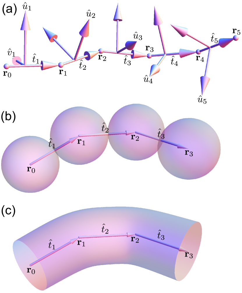
Figure 1: (Color online) WLC and SAWLC chains. A discrete chain is described by the locations of its joints $\mathbf{r}_{i}$, and a local coordinate system defined by three orthonormal vectors $\hat{u_{i}},\hat{v}_{i},\hat{t}_{i}$ at each link. The vector $\hat{t}_{i}$ points along the direction of the ith link. (a) A WLC chain with 5 links and link length $l=1$. (b) A SAWLC chain with 3 links and $l=w=1$. $\hat{u}_{i}$ and $\hat{v}_{i}$ are not shown. (c) Representation of an ideally modeled chain with finite width.

To account for the finite thickness of the DNA we introduce a second energy contribution. We engulf each joint by a “hard-wall” spherical shell of diameter $w$. This allows us to model the final contribution to the elastic energy as a set of hard-wall potentials. For the simple case in which the chain link length is larger than the link diameter ($l\geq w$), and therefore no two neighboring hard-wall spheres overlap, the hard-wall potential energy for the $i$th chain link can be defined as

$$E_{i}^{hw}\left(\left\{\theta_{i},\phi_{i}\right\}\right)=\begin{cases}\infty&\,\,\,\,\mbox{joint $i$ overlaps with one}\\ &\,\,\,\,\mbox{or more joints }0..\left(i-1\right)\\ 0&\,\,\,\,\mbox{otherwise}\end{cases}.$$ (3)

This allows us to write an expression for the total elastic energy associated with the chain of spheres as follows:

$$E\left(\left\{\theta_{N},\phi_{N}\right\}\right)=\sum_{i=1}^{N}E^{el}\left(\theta_{i},\phi_{i}\right)+\sum_{i=1}^{N}E_{i}^{hw}\left(\left\{\theta_{i},\phi_{i}\right\}\right).$$ (4)

We emphasize that this approach (Fig. 1(b)) is an approximation for the more realistic uniformly thick chain (Fig. 1(c)). We choose it for our model due to its simplicity and adequate approximation of the chain excluded volume. However, it may result in incorrect representation of chain excluded volume near the chain termini. In particular, if we compare Fig. 1(c) to Fig. 1(b), we note that the minimally possible end-to-end distance of the chain is $0$ in the former and $w$ in the latter representations, respectively.

The configurational partition function for the model DNA chain consisting of $N$ links is defined as

$$Z_{N} = \int\limits_{-1}^{1}\mbox{d}\cos\theta_{1}\int\limits_{0}^{2\pi}\mbox{d}\phi_{1}\cdots$$ (5)

$$\!\!\!\!\!\int\limits_{-1}^{1}\mbox{d}\cos\theta_{N}\int\limits_{0}^{2\pi}\mbox{d}\phi_{N}\exp\left[-\beta E\left(\left\{\theta_{N},\phi_{N}\right\}\right)\right],$$

where $\beta=\frac{1}{k_{b}T}$. Substituting $E_{i}^{hw}$ from Eq. (3) and opening the sums yields:

$$Z_{N}=\!\!\int\limits_{-1}^{1}\!\!\mbox{d}\cos\theta_{1}\!\int\limits_{0}^{2\pi}\!\!\mbox{d}\phi_{1}\exp\left[-\beta E_{1}^{el}\left(\theta_{1},\phi_{1}\right)\right]\Theta_{1}^{hw}\left(\left\{\theta_{1},\phi_{1}\right\}\right)\cdots\!\!\int\limits_{-1}^{1}\!\!\mbox{d}\cos\theta_{N}\!\int\limits_{0}^{2\pi}\!\!\mbox{d}\phi_{N}\exp\left[-\beta E_{1}^{el}\left(\theta_{N},\phi_{N}\right)\right]\Theta_{N}^{hw}\left(\left\{\theta_{N},\phi_{N}\right\}\right),$$ (6)

where

$$\Theta_{i}^{hw}\left(\left\{\theta_{i},\phi_{i}\right\}\right)=\begin{cases}0&\,\,\,\,\mbox{joint $i$ overlaps with one}\\ &\,\,\,\,\mbox{or more joints}\,0..\left(i-1\right)\\ 1&\,\,\,\,\mbox{otherwise}\end{cases}.$$ (7)

We term the model described by Eq. (4) the self-avoiding worm-like chain model (SAWLC).

II.2 Generalizing the J-factor for the SAWLC

The process of cyclization jacobson_intramolecular_1950 , defined as the joining of one end of the molecule upon itself, can be quantified by the equilibrium constant for the following process jacobson_intramolecular_1950 ; flory_macrocyclization_1966 ; flory_macrocyclization_1976 :

$$M_{2N}\rightleftharpoons M_{N}+cM_{N},$$ (8)

where $\mathit{M_{N},}\,M_{2N}$ and $\mathit{cM_{N}}$ correspond to the monomeric, dimeric (defined as the end-to-end joining of two separate molecules), and cyclized polymer with $N$ links, respectively. This process can be equivalently expressed as two intermediate processes:

$$M_{N}+M_{N} \rightleftharpoons M_{2N}\,,$$ (9a)

$$M_{N} \rightleftharpoons cM_{N}\,.$$ (9b)

The Jacobson-Stockmayer factor (or J-factor) is defined as the equilibrium constant for the entire process (8) jacobson_intramolecular_1950 ; flory_macrocyclization_1976 :

$$J\equiv\frac{\left[M_{N}\right]\left[cM_{N}\right]}{\left[M_{2N}\right]},$$ (10)

and the equilibrium constants for the intermediate processes are similarly defined as

$$K_{D} \equiv \frac{\left[M_{2N}\right]}{\left[M_{N}\right]^{2}},$$ (11)

and

$$K_{C}\equiv\frac{\left[cM_{N}\right]}{\left[M_{N}\right]},$$ (12)

which implies that

$$J\equiv\frac{K_{C}}{K_{D}}.$$ (13)

Eq. 23 is a useful expression for the J-factor from an experimental perspective, but less convenient for numerical simulation.

In order to derive a more insightful expression for $J$, we must first set a geometrical definition for bond formation between the two termini in a chain of finite thickness. We denote the locations of the bonding termini by $\mathbf{r}_{0}$ and $\mathbf{r}_{N}$ , and the directions of their bonds as $\hat{t}_{1}$ and $\hat{t}_{N}$ (Fig. 1), regardless of whether these termini are part of the same chain (i.e. cyclization) or different chains (i.e. dimerization). We define the minimal possible separation between the two termini as $d_{min}$. This leads to the following general bond formation conditions for the SAWLC model (Fig. 2):

• $\mathbf{r}_{N}$ is confined to a volume $\delta\mathbf{r}$ around $\mathbf{r}_{0}$, which is defined by a thin shell between $d_{min}$ and $d_{min}+\varepsilon$ and a solid angle $\delta\omega^{\prime}$ around $-\hat{t}_{1}$. (14)

• $\hat{t}_{N}$ is collinear with $\hat{t}_{1}$ within the range $\delta\omega$. (15)

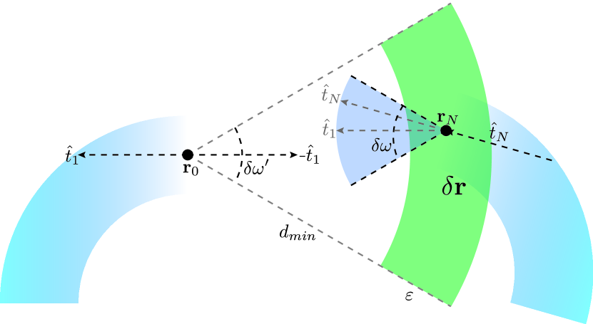
Figure 2: (Color online) Illustration of bond formation criteria. The termini and their bond directions are denoted by $\mathbf{r}_{0},\mathbf{r}_{N}$ and $\hat{t}_{1},\hat{t}_{N}$ respectively. The minimal possible separation between the termini is denoted by $d_{min}$. The cross-section of the volume $\delta\mathbf{r}$ in which $\mathbf{r}_{N}$ must reside is shown as a green (dark gray) wedge. The possible directions for $\hat{t}_{N}$ are shown as a blue (light gray) cone with its base at $\mathbf{r}_{N}$. The rest of the chain is shown schematically with blue (light gray) arcs.

This definition is an extension of the corresponding bond-formation condition defined by Flory flory_statistical_1969 for the WLC. Note that our definition reduces to the Flory criterion when we set $d_{min}=0\,\mbox{and}\,\delta\omega^{\prime}=4\pi$. The motivation for extending the Flory condition arises from our imperfect understanding of DNA bond formation. For example, if the transient bonds formed in (9a) and (9b) are identical to the bonds that comprise the bulk of the chain, then the correct representation of the chain would have to be the one presented in Fig. 1(c) with $d_{min}=0$. If, however, the termini have a repulsive interaction below some separation $d_{min}$, then $d_{min}>0$, as shown for the hard-wall interaction in Fig. 1(b).

Using our geometrical definition for bonding, we can now consider the process in (9a). Before dissociation occurs, $\mathbf{r}_{N}$ is confined to a volume $\delta\mathbf{r}$ around $\mathbf{r}_{0}$. In that volume the orientation of the bond direction $\hat{t}_{N}$ is further restricted by a solid angle of $\delta\omega$ around $\hat{t}_{1}$. After the dissociation, it can be anywhere in volume $v$, and its bond can assume any angle within $4\pi$. Denoting the symmetry number of a cyclic chain species $\sigma_{a}$, we obtain the following change in configurational entropy due to process (9a):

$$\Delta S_{\left(a\right)}=R\ln\left(\frac{4\pi v/\sigma_{a}}{\delta\mathbf{r}\delta\omega}\right)=R\ln\left(\frac{V}{N_{A}\sigma_{a}\delta\mathbf{r}\frac{\delta\omega}{4\pi}}\right),$$ (16)

where we denote the change in entropy as $\Delta S_{\left(a\right)}$, and the volume per mole as $V$ resulting in $v=\frac{V}{N_{A}}$ as the volume per one molecule, where $N_{A}$ is Avogadro’s number. If, for simplicity, we assume that the species are present in standard state concentration of one mole per unit volume ($V=1$), we obtain

$$\Delta S_{\left(a\right)}=R\ln\left(\frac{1}{N_{A}\sigma_{a}\delta\mathbf{r}\frac{\delta\omega}{4\pi}}\right).$$ (17)

The standard molar Gibbs free-energy change for the dimerization process (9a) can be written as

$$\Delta G_{\left(a\right)}^{\circ}=\Delta H_{\left(a\right)}^{\circ}-RT\ln\left(\frac{1}{N_{A}\sigma_{a}\delta\mathbf{r}\frac{\delta\omega}{4\pi}}\right),$$ (18)

where $\Delta H_{\left(a\right)}^{\circ}$ is the dissociation heat of the dimer.

In the cyclization process (9b) an intramolecular bond is formed which is equivalent to the one severed in the dimerization (9a). We assume here that $\Delta H_{\left(b\right)}^{\circ}=-\Delta H_{\left(a\right)}^{\circ}$ where $\Delta H_{\left(b\right)}^{\circ}$ is the dissociation heat of the ring. This assumption is valid unless the overall length of the chain is so small as to induce strainflory_statistical_1969 . For the computation of the change in configurational entropy due to process (9b), $\Delta S_{\left(b\right)}$, we note that the termini of chain $M_{N}$ must meet within the same ranges of $\delta\mathbf{r}$ and $\delta\omega$ as defined in Eqs. (• ‣ II.2)-(• ‣ II.2). This implies that the probability for the termini to meet is given by

$$\int\limits_{\delta\mathbf{r}}\int\limits_{\delta\omega}\mathbf{C}\left(\mathbf{r},\omega\right)\mbox{d}\mathbf{r}\mbox{d}\omega,$$ (19)

where $\mathbf{C}\left(\mathbf{r},\omega\right)$ is the function expressing the distribution of the end-to-end vector $\mathbf{r}\equiv\mathbf{r}_{N}-\mathbf{r}_{0}$ within a solid angle $\omega$ around $\hat{t}_{1}$ ($\frac{\omega}{2\pi}\equiv\hat{t}_{1}\cdot\hat{t}_{N}$), per unit range in $\mathbf{r}$ $\left(\int\limits_{v}\int\limits_{4\pi}\mathbf{C}\left(\mathbf{r},\omega\right)d\mathbf{r}d\omega=1\right)$. Thus, the change in configurational entropy in process (9b) is

$$\Delta S_{\left(b\right)}=R\ln\left(\int\limits_{\delta\mathbf{r}}\int\limits_{\delta\omega}\mathbf{C}\left(\mathbf{r},\omega\right)\mbox{d}\mathbf{r}\mbox{d}\omega\frac{\sigma_{a}}{\sigma_{R_{N}}}\right),$$ (20)

where $\sigma_{R_{N}}$ is the symmetry number of a ring of $N$ links. Hence

$$\Delta G_{\left(b\right)}^{\circ}=\Delta H_{\left(b\right)}^{\circ}-RT\ln\left(\int\limits_{\delta\mathbf{r}}\int\limits_{\delta\omega}\mathbf{C}\left(\mathbf{r},\omega\right)\mbox{d}\mathbf{r}\mbox{d}\omega\,\frac{\sigma_{a}}{\sigma_{R_{N}}}\right).$$ (21)

Adding the Gibbs free energy change for processes (9a) and (9b), we obtain the change in the Gibbs free energy for the entire process (8):

$$\Delta G = -T\left(\Delta S_{\left(a\right)}+\Delta S_{\left(b\right)}\right)$$ (22)

$$= -RT\ln\left(\frac{\int\limits_{\delta\mathbf{r}}\int\limits_{\delta\omega}\mathbf{C}\left(\mathbf{r},\omega\right)\mbox{d}\mathbf{r}\mbox{d}\omega}{N_{A}\sigma_{R_{N}}\delta\mathbf{r}\frac{\delta\omega}{4\pi}}\right).$$

This allows us to extract the J-factor:

$$J=\frac{4\pi\int\limits_{\delta\mathbf{r}}\int\limits_{\delta\omega}\mathbf{C}\left(\mathbf{r},\omega\right)\mbox{d}\mathbf{r}\mbox{d}\omega}{N_{A}\sigma_{R_{N}}\delta\mathbf{r}\delta\omega}.$$ (23)

Finally, when taking the infinitely thin or WLC limit for long chains ($L\gg b$), we can assume that around $\mathbf{r}=0$, $\mathbf{C}\left(\mathbf{r},\omega\right)\approx\frac{\mathbf{C}\left(0\right)}{4\pi}$ is approximately uniform and independent of $\omega$. Defining $\delta\mathbf{r}$ by $d_{min}=0$ and $\delta\omega^{\prime}=4\pi$, while taking $\delta\mathbf{r}\rightarrow 0$, the expression above reduces to

$$J=\frac{4\pi\int\limits_{\delta\mathbf{r}}\int\limits_{\delta\omega}C\left(\mathbf{r},\omega\right)\mbox{d}\mathbf{r}\mbox{d}\omega}{N_{A}\sigma_{R_{N}}\delta\mathbf{r}\delta\omega}\approx\frac{\mathbf{C}\left(0\right)\delta\mathbf{r}\delta\omega}{N_{A}\sigma_{R_{N}}\delta\mathbf{r}\delta\omega}=\frac{\mathbf{C}\left(0\right)}{N_{A}\sigma_{R_{N}}},$$ (24)

which is the original expression by Flory flory_statistical_1969 for the WLC J-factor. Note that for the case of DNA cyclization $\sigma_{R_{N}}=1$ semlyen_cyclic_2000 . We use the expression in Eq. (23) to compute the J-factor by numerical simulation.

III Numerical Implementation of SAWLC

III.1 Numerical implementation overview

In order to evaluate the SAWLC looping probabilities, we developed a Monte-Carlo algorithm that is capable of generating a large number of plausible self-avoiding DNA chains. The Monte-Carlo simulation was written in CUDA C++, and was executed on two NVIDIA GeForce GTX TITAN cards. The length of the generated chains ranged from $50$ to $5000$ links. Each chain in our ensemble was grown one link at a time by selecting the link’s orientation according to the distribution described in Sec. III.2, taking into account disallowed directions due to the excluded volume of previous links. In addition, each completed chain was assigned a Rosenbluth weight as described in Sec. III.3, resulting in a faithful representation of the full configurational space. Typical sizes of generated ensembles were $N_{c}\approx 10^{10}$ chains.

We computed the mean-square end-to-end distance $\left\langle R^{2}\right\rangle$ and the polymer end-to-end separation power-law exponent $\nu$ ($\sqrt{\left\langle R^{2}\right\rangle}\propto\mathit{N^{\nu}}$) in order to compare our simulation to previous results clisby_accurate_2010 ; chen_renormalization-group_1992 . For the computation of the J-factor, we computed the function $\mathbf{C}\left(\mathbf{r},\omega\right)$ describing the distribution of the end-to-end vector $\mathbf{r}$ with angle $\omega$ from $\hat{t}_{1}$ (see Eq. 23). The procedures used in the computation of these expressions are detailed in Sec. III.3.

In the following, we denote the number of links in the simulated chain by $N$, the length of the links by $l$, the length of the chain by $L\equiv Nl$, the diameter (or width) of the chain by $w$ and the Kuhn length of the corresponding WLC as $b$, where $b$ is given by tree_is_2013 :

$$\frac{b}{l}=\left(\frac{a-1+a\coth a}{a+1-a\coth a}\right),$$ (25)

and where $a$ is the bending constant of the chain.

III.2 Sampling of chain angles

Our goal was to sample angles $\theta_{i},\phi_{i}$ that satisfy the probability distribution

$$P_{i}^{\theta,\phi}\left(\cos\theta_{i}\epsilon\left[-1,1\right];\,\phi_{i}\epsilon[0,2\pi)\right)\propto\\ \exp\left[-\beta E^{el}\left(\theta_{i},\phi_{i}\right)\right]\Theta_{i}^{hw}\left(\left\{\theta_{i},\phi_{i}\right\}\right)=\\ \exp\left[a\left(1-\cos\theta_{i}\right)\right]\Theta_{i}^{hw}\left(\left\{\theta_{i},\phi_{i}\right\}\right)$$ (26)

Ṅote that we sampled $\cos\theta_{i}$ and not $\theta_{i}$ according to this distribution, since the quantity that is distributed uniformly over the unit sphere is $\cos\theta_{i}$ and not $\theta_{i}$.

We chose to sample the $i$th link’s orientation angles $\left(\cos\theta_{i},\phi_{i}\right)$ using inversion sampling devroye_non-uniform_1986 . Here the inversion sampling of a single random variable $X$ from a probability distribution function ($PDF\left(X\right)$) is carried out by, first, integrating the $PDF\left(X\right)$ over the entire range of $X$, resulting in a cumulative distribution function ($CDF\left(X\right)$). Then, a random number $y$ in the range $\left(0,1\right)$ is generated from a continuous uniform distribution. Finally, the desired variable value $x$ is extracted from the inverse function of the $CDF\left(X\right)$ at y, i.e. $x=CDF^{-1}\left(y\right)$. In the case discussed here, the two-dimensional variable space $\left(\cos\theta_{i},\phi_{i}\right)$ can be mapped to a one-dimensional space due to azimuthal symmetry considerations in the elastic energy. We computed the $CDF\left(X\right)$ numerically, using the adaptive Gaussian integration method, pieper_recursive_1999 and subsequently inverted it.

In order to show how the mapping from the two-dimensional variable space $\left(\cos\theta_{i},\phi_{i}\right)$ to a one-dimensional space is carried out, we first consider the case of the chain without the excluded volume constraint. Namely, we compute the inverse of the following function:

$$I\left(\cos\theta_{i}\right)=\frac{\int\limits_{-1}^{\cos\theta_{i}}\mbox{d}\cos\theta\int\limits_{0}^{2\pi}\mbox{d}\phi\,e^{-a\left(1-\cos\theta\right)}}{\int\limits_{-1}^{1}\mbox{d}\cos\theta\int\limits_{0}^{2\pi}\mbox{d}\phi\,e^{-a\left(1-\cos\theta\right)}},$$ (27)

which allows us to extract $\cos\theta_{i}$, provided that some random number $y$ corresponding to $I\left(\cos\theta_{i}\right)$ is generated in the range $\left(0,1\right)$. Finally, we generate $\phi_{i}$ from a uniform distribution over the entire range $\phi_{i}\epsilon[0,2\pi)$ to complete the two-angle set.

If we reintroduce the hard-wall potential, the above integral now changes to:

$$I\left(\cos\theta_{i}\right)=\frac{\int\limits_{-1}^{\cos\theta_{i}}\mbox{d}\cos\theta\int\limits_{allowed\,\phi\,for\,\theta}\mbox{d}\phi\,e^{-a\left(1-\cos\theta\right)}}{\int\limits_{-1}^{1}\mbox{d}\cos\theta\int\limits_{allowed\,\phi\,for\,\theta}\mbox{d}\phi\,e^{-a\left(1-\cos\theta\right)}}.$$ (28)

The integral over $\phi$ is no longer over the entire $[0,2\pi)$ range, as some directions in space cannot be assumed by the new link due to the excluded volume constraint. Thus, for each possible $\theta$ angle of the new link, there is a different range of $\phi$ values that are allowed. The situation is illustrated in Fig. 3. The red sphere is an object in close proximity to the endpoint of the $\left(i-1\right)$th link. The black cone maps the directions forbidden for $\hat{t}_{i}$, as that would cause an overlap between the $i$th link and the red sphere. These directions must be excluded from the integration in (28). As a result, we may proceed similarly to the non-constrained case, except that in this case the angle $\phi_{i}$ is no longer sampled from the full $[0,2\pi)$ range, but from a smaller range of possible values.

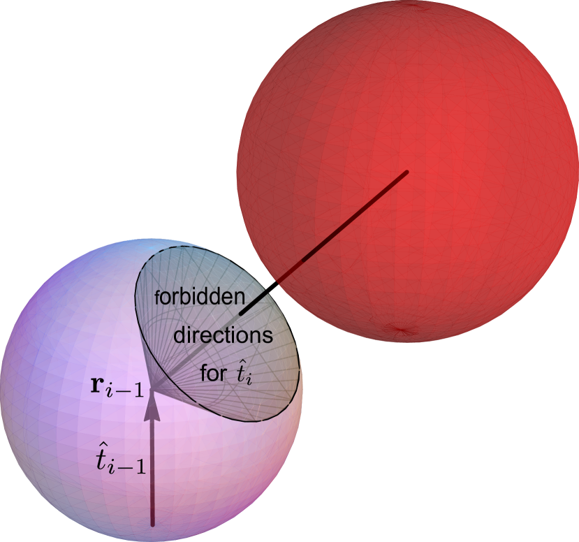
Figure 3: (Color online) Forbidden directions for $\hat{t}_{i}$. Purple (light gray) sphere is the excluded volume around $\mathbf{r}_{i-1}$ (the endpoint of the $(i-1)$th link). The red (dark gray) sphere is a potentially colliding object. If $\hat{t}_{i}$ assumes any direction inside the black (dark gray) cone this would result in a collision of the hard-wall sphere at $\mathbf{r}_{i}$ with the red sphere.

In order to compute the integral in (28) and to generate $\phi_{i}$, we first compute the set of values that are allowed for $\phi_{i}$ for each value of $\theta_{i}$. Since there can be more than one colliding object, the set of allowed values for $\phi_{i}$ need not be one continuous range. Rather, these values can be organized into $m\geq 1$ consecutive ranges $[r_{i,0}^{a},r_{i,0}^{b}],...,[r_{i,m-1}^{a},r_{i,m-1}^{b}]$, such that

$$\phi{}_{i}^{tot}=\sum_{j=0}^{m-1}\left(r_{i,j}^{b}-r_{i,j}^{a}\right)\leq 2\pi.$$ (29)

Thus, for each $\theta_{i}$ the $\phi_{i}$ angle can be sampled from a stepwise uniform distribution:

$$P_{i}^{\phi}\left(\theta_{i},\,\phi_{i}\epsilon(0,2\pi)\right)=\frac{\sum\limits_{j=0}^{m-1}\Theta\left(\phi_{i}-r_{i,j}^{a}\right)\Theta\left(r_{i,j}^{b}-\phi_{i}\right)}{\phi{}_{i}^{tot}}.$$ (30)

III.2.1 Mapping disallowed directions for the $i$th link

After generating $i-1$ links of the chain, the endpoint is located at $\mathbf{r}_{i-1}$ and the link direction is $\hat{t}_{i-1}$. We now have to map all the directions that $\hat{t}_{i}$ cannot assume (as shown in Fig. 3). In the following discussion we focus on one of the chain joints in the vicinity of $\mathbf{r}_{i-1}$ which limits the range of $\hat{t}_{i}$. We denote the location of this potentially colliding joint as $\mathbf{r}_{p}$ and the vector from the endpoint $\mathbf{r}_{i-1}$ to the center of the potentially colliding sphere as $\mathbf{r}$:

$$\mathbf{r}=\mathbf{r}_{p}-\mathbf{r}_{i-1}.$$ (31)

We denote by $\gamma$ the angle between the direction of the last link $\hat{t}_{i-1}$ and $\mathbf{r}$:

$$\cos\gamma=\frac{\mathbf{r}}{\left|\mathbf{r}\right|}\cdot\hat{t}_{i-1}.$$ (32)

We note that the forbidden directions for $\hat{t}_{i}$ form a cone around $\mathbf{r}$ (Fig. 3). We denote half of the opening angle of the cone by $\alpha$ which can then be calculated from simple geometrical considerations as:

$$\cos\alpha=\frac{\left|\mathbf{r}\right|^{2}-w^{2}+l^{2}}{2\left|\mathbf{r}\right|l}.$$ (33)

A certain $\left(\theta_{i},\phi_{i}\right)$ direction is disallowed for $\hat{t}_{i}$ if the vector $\mathbf{r}_{i}=\mathbf{r}_{i-1}+l\hat{t}_{i}$ is at a distance $\left|\mathbf{r}-\mathbf{r}_{i}\right|^{2}\leq w^{2}$ from $\mathbf{r}_{p}$. We proceed to work in the local coordinates of the $\left(i-1\right)$th link, assuming for now that $\mathbf{r}$ is in the XZ plane in these coordinates:

$$\mathbf{r} = \left|\mathbf{r}\right|\left(\sin\gamma,0,\cos\gamma\right),$$ (34)

$$\mathbf{r}_{i}=l\hat{t}_{i} = l(\sin\theta_{i}\cos\phi_{i},\sin\theta_{i}\sin\phi_{i},\cos\theta_{i}).$$ (35)

Disallowed values of $\left(\theta_{i},\phi_{i}\right)$ satisfy the following inequality:

$$\left|\mathbf{r}-\mathbf{r}_{i}\right|^{2}=(\left|\mathbf{r}\right|\sin\gamma-l\sin\theta_{i}\cos\phi_{i})^{2}+\\ (\left|\mathbf{r}\right|\cos\gamma-l\cos\theta_{i})^{2}+l^{2}\sin^{2}\theta_{i}\sin^{2}\phi_{i}\leq w^{2}.$$ (36)

We can thus map the disallowed range for $\hat{t}_{i}$ in two steps. We first determine the range of $\cos\theta_{i}$ for which a collision can occur at all. Then, for each $\theta_{i}$ in this range we determine the range of $\phi_{i}$ for which a collision does occur.

III.2.2 The $\theta_{i}$ range for which a collision occurs

The critical values $\cos\theta_{\pm}$ for which $\left|\mathbf{r}-\mathbf{r}_{i}\right|^{2}=w^{2}$ can be derived from Eq. (36):

$$\cos\theta_{\pm}=\cos\left(\gamma\mp\alpha\right)=\cos\gamma\cos\alpha\pm\sin\gamma\sin\alpha.$$ (37)

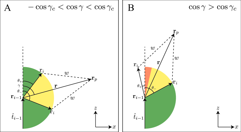
Figure 4: (Color online) $\theta_{i}$ ranges mapping. $\theta_{i}$ ranges that do not cause a collision for all values of $\phi_{i}$ are marked in green (dark gray). $\theta_{i}$ ranges that cause a collision for some values of $\phi_{i}$ are marked in yellow (light gray). $\theta_{i}$ ranges that cause a collision for all values of $\phi_{i}$ are marked in red (medium gray). (a) If $\theta_{i}\in[\theta_{+},\theta_{-}]$, a collision occurs for some values of $\phi_{i}$. (b) If $\theta_{i}\in[0,\theta_{+}]$, a collision occurs for all values of $\phi_{i}$.

Caution is needed when interpreting the results in (37). It is true that choosing $\cos\theta_{i}\in\left[\cos\theta_{-},\cos\theta_{+}\right]$ will result in collision for some values of $\phi_{i}$ (Fig. 4). However, this does not take into account additional $\theta_{i}$ ranges for which there is a collision for all values of $\phi_{i}$. Such a situation is shown in Fig. 4(b): for $\cos\theta_{i}\in\left[\cos\theta_{-},\cos\theta_{+}\right]$ obviously a collision occurs for some values of $\phi_{i}$, but for $\cos\theta_{i}\in\left[\cos\theta_{+},1\right]$ a collision occurs for all values of $\phi_{i}$.

If the colliding object is located at $\cos\gamma>\cos\alpha$ or at $\cos\gamma<-\cos\alpha$ there is a range of $\theta_{i}$ values for which a collision occurs for all values of $\phi_{i}$. To summarize:

• There are disallowed $\phi_{i}$ angles for $\cos\theta_{i}\in[\cos\theta_{-},\cos\theta_{+}]$.

• If $\cos\gamma>\cos\alpha$, for $\cos\theta_{i}\in[\cos\theta_{+},1]$ there is always a collision.

• If $\cos\gamma<-\cos\alpha$, for $\cos\theta_{i}\in[-1,\cos\theta_{-}]$ there is always a collision.

III.2.3 The $\phi_{i}$ range in which a collision occurs, for specific $\theta_{i}$

We begin with Eq. (36) and find the critical value of $\phi_{i}$ ($\phi_{ic}$) for a specific value of $\theta_{i}$:

$$\cos\phi_{ic}\left(\theta_{i}\right)=\frac{\cos\alpha-\cos\gamma\cos\theta_{i}}{\sin\gamma\sin\theta_{i}}.$$ (38)

A full collision (no possible values for $\phi_{ic}$) occurs when

$$\frac{\cos\alpha-\cos\gamma\cos\theta_{i}}{\sin\gamma\sin\theta_{i}} < -1.$$ (39)

No collision occurs when

$$\frac{\cos\alpha-\cos\gamma\cos\theta_{i}}{\sin\gamma\sin\theta_{i}} > 1.$$ (40)

The disallowed angles for a specific $\theta_{i}$ are:

$$-\phi_{ic}\left(\theta_{i}\right)\leq\phi_{disallowed}\left(\theta_{i}\right)\leq\phi_{ic}\left(\theta_{i}\right).$$ (41)

We can now generalize to the case when $\mathbf{r}$ is not in the XZ plane. If $\mathbf{r}=\left|\mathbf{r}\right|\left(\sin\gamma\cos\beta,\sin\gamma\sin\beta,\cos\gamma\right)$ then

$$\beta-\phi_{ic}\left(\theta_{i}\right)\leq\phi_{disallowed}\left(\theta_{i}\right)\leq\beta+\phi_{ic}\left(\theta_{i}\right).$$ (42)

III.3 Faithful ensemble sampling

For the simulation of the WLC model we used importance sampling (IS, see Appendix A.1). For the simulation of the SAWLC model (and the thick freely-jointed self-avoiding chain) we used weighted-biased sampling (WBS, see Appendix A.2) prigogine_monte_1998 , which is based on a method developed by Rosenbluth and Rosenbluth rosenbluth_monte_1955 . A variation of this method was recently used to sample dsDNA configurational space tree_is_2013 for much longer chains than the ones used in this work to examine the cyclization process.

The partition function for an ensemble of $N_{c}$ sampled chains of $N$ links in WBS is given by

$$Z_{N}=\sum_{j=1}^{N_{c}}W\left(\left\{\theta_{N},\phi_{N}\right\}_{j}\right),$$ (43)

where $W\left(\left\{\theta_{N},\phi_{N}\right\}_{j}\right)$ is the Rosenbluth factor of the $j$th chain in the ensemble:

$$W\left(\left\{\theta_{N},\phi_{N}\right\}\right)=\prod_{i=1}^{N}\int\limits_{-1}^{1}\mbox{d}\cos\theta_{i}\int\limits_{0}^{2\pi}\mbox{d}\phi_{i}\exp\left[-\beta E^{el}\left(\theta_{i},\phi_{i}\right)\right]\Theta_{i}^{hw}\left(\left\{\theta_{i},\phi_{i}\right\}\right)=\prod_{i=1}^{N}\!\!\!\!\!\!\!\!\!\!\!\!\!\!\!\!\!\!\int\limits_{non-colliding\,directions}\!\!\!\!\!\!\!\!\!\!\!\!\!\!\!\!\!\!\mbox{d}\theta_{i}\mbox{d}\phi_{i}\exp\left[-\beta E^{el}\left(\theta_{i},\phi_{i}\right)\right],$$ (44)

with $\Theta_{i}^{hw}$ defined in eq. (7).

The average value $\left\langle f\right\rangle$ of a physical property is calculated as:

$$\left\langle f\right\rangle=\frac{\sum\limits_{j=1}^{N_{c}}f\left(\left\{\theta_{N},\phi_{N}\right\}_{j}\right)W\left(\left\{\theta_{N},\phi_{N}\right\}_{j}\right)}{\sum\limits_{j=1}^{N_{c}}W\left(\left\{\theta_{N},\phi_{N}\right\}_{j}\right)}.$$ (45)

This allows the computation of $\left\langle R^{2}\right\rangle$. The power-law exponent $\nu$ was extracted from the computed $\left\langle R^{2}\right\rangle$ (see Appendix B.1).

To approximate $C\left(\mathbf{r},\omega\right)$, the configurational space for $\mathbf{r}=\left(r,\omega^{\prime}\right)$ and $\omega$ is partitioned into bins, with bin volume $\mbox{d}\mathbf{r}\times\mbox{d}\omega$. In each bin we compute the probability of the end-to-end vector $\mathbf{r}$ and relative bond orientation to be contained in the bin:

$$P_{bin}\left(r,\omega^{\prime},\omega\right)=\lim_{N_{c}\rightarrow\infty}\frac{\sum\limits_{j=1}^{N_{c}}f_{bin}\left(\mathbf{r},\omega,\left\{\theta_{N},\phi_{N}\right\}_{j}\right)W\left(\left\{\theta_{N},\phi_{N}\right\}_{j}\right)}{\sum\limits_{j=1}^{N_{c}}W\left(\left\{\theta_{N},\phi_{N}\right\}_{j}\right)}$$ (46)

where

$$f_{bin}\left(\mathbf{r},\omega,\left\{\theta_{N},\phi_{N}\right\}\right) = \begin{cases}1&\,\,\,\,\mbox{$\mathbf{r}_{N}$ and $\hat{t}_{N}$ relative to $\hat{t}_{1}$ are contained}\\ &\,\,\,\,\mbox{ in the bin defined by $\mathbf{r}$,$\omega$\ and $\mathbf{\mbox{d}r}$,d$\omega$}\\ 0&\,\,\,\,\mbox{otherwise}\end{cases}.$$ (47)

$C\left(\mathbf{r},\omega\right)$ is then computed by

$$C\left(\mathbf{r},\omega\right)=\frac{P_{bin}\left(r,\omega^{\prime},\omega\right)}{\mbox{d}\mathbf{r}\times\mbox{d}\omega}.$$ (48)

IV Results

IV.1 DNA end-to-end distance analysis and comparison to RG results

In order to verify that our algorithm generates a faithful swollen chain ensemble, we simulated chains of up to 5000 links and compared our simulation results to previously-published renormalization group (RG) calculations chen_renormalization-group_1992 and Monte-Carlo results tree_is_2013 . We simulated chains with the touching-beads model ($l=w$, see Fig. 1(b)) and dsDNA-like parameters of $b\approx 106\mbox{ nm}$ and $w\approx 4.6\mbox{ nm}$.

In Fig. 5 we plot the RG predictions and our simulation results for the polymer end-to-end separation power-law exponent $\nu$ as a function of the normalized chain length $\frac{L}{b}$. We display three cases: a “thick” polymer with dsDNA-like parameters $\frac{w}{b}\approx\frac{4.6}{106}\ll 1$ (SAWLC), a zero-thickness dsDNA (WLC) and a fully flexible “thick” polymer with $\frac{w}{b}=1$ (self-avoiding freely-jointed chain, SAFJC). The simulation shows that the SAWLC (dashed green curve and green squares) maintains a WLC-like behavior (dotted red curve and red diamonds) for lengths that are up to several times larger than the persistence length $l_{P}\equiv\frac{b}{2}$. At $\frac{L}{b}\approx 30$ the curve and simulation begin to bend up and approach the SAFJC prediction until convergence of the SAWLC and the SAFJC is predicted to occur by RG at $\frac{L}{b}\approx 10^{4}$. It is important to note that while our simulation does not capture the exact convergence to the predicted SAWLC behavior due to chain-length limitations of our algorithm, the trends are precisely tracked over the range of the RG predictions. Moreover, the length at which the divergence away from the WLC behavior occurs (the length where the dashed green and dotted red lines separate) is highly dependent on the width parameter $\left(\frac{w}{b}\right)$. This result is consistent with experimental observations nepal_structure_2013 and simulation tree_is_2013 .

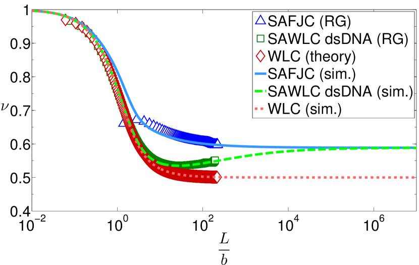
Figure 5: (Color online) Comparison of the simulation results to the RG calculations and WLC theory. Power-law exponent $\nu$ of the end-to-end distance $\sqrt{\langle R^{2}\rangle}$ is plotted as a function of chain length $L/b$. We compare three cases (top to bottom): a feely-jointed “thick” polymer (SAFJC) with $\frac{w}{b}=1$ and $l=w$ (solid blue line - RG and blue triangles - simulation), a “thick” polymer (SAWLC) with dsDNA-like parameters $\frac{w}{b}=\frac{4.6}{106}\ll 1$ and $l=w$ (dashed green line - RG and green squares - simulation), and a zero-thickness dsDNA (WLC) with $\frac{l}{b}=\frac{4.6}{106}$ (dotted red line - WLC and red diamonds - simulation). The excluded volume parameter in the RG calculations was rescaled to match the excluded volume in the simulations with $\overline{u}_{RG}=1.5u$ following Tree et. al. tree_is_2013 .

For the case of the SAFJC $\left(\frac{w}{b}=1\right)$, our simulation produces a decaying power law that converges to the Flory prediction of $\sqrt{\langle R^{2}\rangle}\propto N^{-0.5876}$ for long chain lengths. Note that our simulation for the semi-flexible chain deviates from the RG predictions only for very short chains ($N<5$). However, for the fully flexible chain our simulation converges on the RG predictions for values $N>20$. These deviations are a natural consequence of the discrete simulation process, as our simulation employs finite size links while the RG and WLC predictions are for continuous chain models, which correspond to the case $l\rightarrow 0$ and $N\rightarrow\infty$. The larger short-scale deviation from the RG predictions generated by our simulation for the SAFJC (deviation of the blue triangles from the solid blue line for $\frac{L}{b}<10^{2}$) can be explained by short-range excluded volume interactions, which are properly simulated by our algorithm and are for the most part neglected in the RG model chen_renormalization-group_1992 .

IV.2 The SAWLC J-factor in the entropic regime

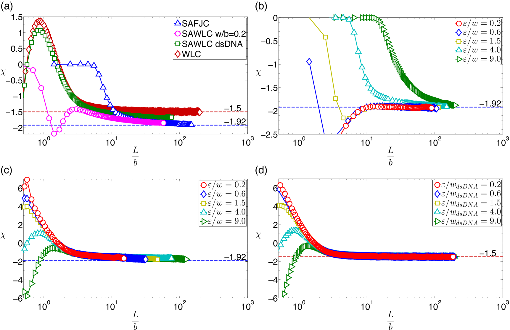
Figure 6: (Color online) The J-factor power law. (a) Comparison of J-factor power-law exponents $\chi$ for the WLC ($\frac{w}{b}=0$) (red diamonds), SAWLCs with $\frac{w}{b}=0.046$ (green squares) and $\frac{w}{b}=0.2$ (magenta circles), and the SAFJC ($\frac{w}{b}=1$) (blue triangles), using $d_{min}=w$ and $\frac{\varepsilon}{w}=4$. The blue(bottom) and red (top) dashed lines correspond to the SAFJC and WLC power laws of $-1.92$ and $-1.5$, respectively. (b)-(d) Effect of $\varepsilon$ on the J-factor power-law exponent. (b) J-factor power-law exponent for the SAFJC with various $\frac{\varepsilon}{w}$. (c) J-factor power-law exponent for the SAWLC with $\frac{\omega}{b}=\frac{4.6}{106}$ and with various $\frac{\varepsilon}{w}$. (d) J-factor power-law exponent for the WLC ($\frac{w}{b}=0$) with $b=106$ nm and with various $\frac{\varepsilon}{w_{dsDNA}}$, where $w_{dsDNA}$ is taken to be equal to that of dsDNA.

We next proceeded to model the looping or cyclization J-factor as defined in Eq. (23). We first examined the entropic regime, namely $\frac{L}{b}\gg 1$. For the sake of simplicity, for this regime we set $d_{min}=w$ and $\delta\omega^{\prime}=\delta\omega=4\pi$ in (• ‣ II.2) and (• ‣ II.2). In Fig. 6 we plot the J-factor power-law exponent $\chi$ as a function of the normalized chain length $\frac{L}{b}$. Previous theoretical studies have shown that in the entropic regime, the J-factor scales like $J\propto N^{\chi}=N^{-\frac{3}{2}}$ for the WLC model and $J\propto N^{-\left(3\nu+\gamma-1\right)}=N^{-1.9196}$ for a flexible swollen chain (see Appendix B.2), where $\nu$ is the end-to-end power-law exponent and $\gamma$ is the “universal” exponent gennes_scaling_1979 . In Fig. 6(a), we plot the J-factor power-law exponents for the WLC ($\frac{w}{b}=0$, red diamonds), SAWLCs with $\frac{w}{b}=\frac{4.6}{106}$ (green squares) and $\frac{w}{b}=0.2$ (magenta circles), and the SAFJC ($\frac{w}{b}=1$, blue triangles). The panel shows that the behavior of the power-law exponent dramatically changes as the value of $\frac{w}{b}$ increases from zero for the ideal WLC behavior to one for the fully swollen chain. Both the semi-flexible WLC and the fully-flexible SAWLC J-factors converge on their respective theoretical predictions. Moreover, our calculations indicate that the SAWLC J-factor converges to the asymptotic value of $-1.92$ in a manner which is highly dependent on the thickness of the respective chains.

To gain a better insight into the power-law behavior of the J-factor, we plot in Fig. 6(b)-(d) the J-factor power-law exponents for the SAFJC, the SAWLC with dsDNA aspect ratio $\frac{w}{b}=\frac{4.6}{106}$, and the WLC, for various values of $\frac{\varepsilon}{w}$, corresponding to the size of the sphere where bond formation between the two chain termini occurs (see Eq. • ‣ II.2) divided by the chain diameter. We notice that in all three figures the power-law behavior in the far entropic regime converges to the scaling theory’s predicted limit. Instead, the effects of $\frac{\varepsilon}{w}$ seem to be localized to the shorter range elastic regime and the intermediate (elastic-entropic) transition region. However, the effects of varying $\frac{\varepsilon}{w}$ on the J-factor power-law exponent for the SAFJC are striking as compared with the other cases. Here (Fig. 6(b)) we observe a sharp dependence in the elastic regime. Moreover, the value of $\frac{L}{b}$ at which the transition to the entropic regime and the convergence to the scaling-theory power-law exponent occur, is a strong function of $\frac{\varepsilon}{w}$. Consequently, we conclude that this parameter plays an important role in the physical properties of polymers the closer the value of $\mathit{\frac{w}{b}}$ is to one.

IV.3 The SAWLC J-factor in the elastic regime

In order to complete our description of the effects of the excluded volume on the J-factor, we generated ensembles of short chains up to $\frac{L}{b}\approx 3$. It was previously predicted gennes_scaling_1979 that for short chains the excluded volume effect should be negligible, as the elastic energy is expected to be the dominant contribution to the probability of looping. Fig. 7 shows cross-sections of $\mathbf{C}\left(\mathbf{r}\right)\equiv\int\mathbf{C}\left(\mathbf{r},\omega\right)\mbox{d}\omega$ in the $\mathrm{xz}$ plane for both the WLC and the SAWLC with $\frac{L}{b}\approx\frac{55.2~{}\mathrm{nm}}{106~{}\mathrm{nm}}\approx 0.52$ and $d_{min}=0$ and $\delta\omega^{\prime}=\delta\omega=4\pi$ in the SAWLC case, with $\mathbf{r}_{0}$ at the origin and $\hat{t}_{1}=\hat{z}$. Fig. 7(a)-(b) show that the spatial distributions for the end-to-end separations are highly anisotropic functions in the z-direction for both the SAWLC and the WLC. This implies that the probability of looping itself must be highly anisotropic. In addition, both distributions look similar, where the only significant deviation observed for the self-avoiding from the non-self-avoiding distribution emerges from the space occupied by the chain around the origin (white circle in Fig. 7(b). In order to quantify this observation, we divided the two distributions, as shown in Fig. 7(c). It is evident from this panel that while both the self-avoiding and non-self-avoiding $\mathbf{C}\left(\mathbf{r}\right)$ functions are similar, they differ around the origin in the positive $\mathrm{z}$ direction, where the SAWLC has reduced probability (Fig. 7(d)). This is expected, since $\mathbf{r}_{1}=l\hat{z}$, rendering the volume around the origin inaccessible for $\mathbf{r}_{N}$.

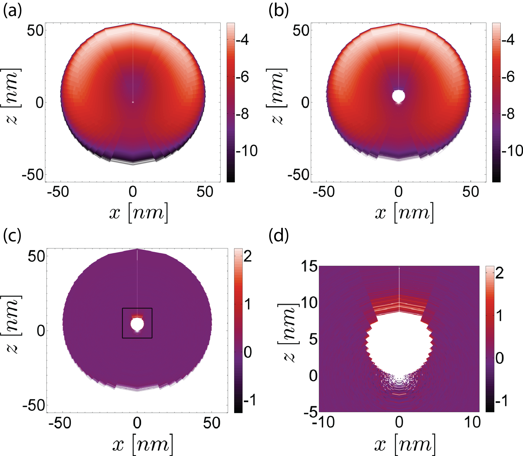
Figure 7: (Color online) WLC and SAWLC ($d_{min}=0$) comparison in the elastic regime. The insets show a cross section of the data in the xz plane. $\mathbf{r}_{0}$ is in the origin and $\hat{t}_{1}=\hat{z}$. (a) $\log_{10}\left(\mathbf{C}_{\mathrm{WLC}}\mathbf{\left(\mathbf{r}\right)}/N_{A}\right)$ in the xz plane for WLC with $L=162$ bp. (b) $\log_{10}\left(\mathbf{C}_{\mathrm{SAWLC-0}}\mathbf{\left(\mathbf{r}\right)}/N_{A}\right)$ in the xz plane for SAWLC with $L=162$ bp, $\frac{w}{b}=\frac{4.6}{106}$ and $d_{min}=0$. (c) $\log_{10}\left(\frac{\mathbf{C}_{\mathrm{WLC}}\mathbf{\left(\mathbf{r}\right)}}{\mathbf{C}_{\mathrm{SAWLC-0}}\mathbf{\left(\mathbf{r}\right)}}\right)$. (d) A blowup of the rectangular section marked in (c). Note, shorter chains were also examined, however, the accumulated statistical data around the origin in those chains was insufficient, and precluded a comprehensive analysis. Qualitatively, however, the shorter chains exhibited the same behavior as shown below in the data ranges that contained significant statistical data.

We next examined the case in which $d_{min}\neq 0$ (and $\delta\omega^{\prime}=\delta\omega=4\pi$), implying that looping is now defined for some finite volume around the origin for the WLC. In the SAWLC model, this condition translates to a larger volume around the origin for which the distribution vanishes (see Fig. 8(a)). However, the actual deviation from the non-self-avoiding WLC distribution function is for the most part negligible, as can be seen from Fig. 8(b), and is similar in its scope to the minimal effect described for $d_{min}=0$ above. Consequently, any deviation of the SAWLC J-factor from the WLC prediction in the elastic regime is not due to some global modification of the underlying distribution, but rather arises from a local redefinition of $\delta\mathbf{r}$ in Eq. (23), which is imperative due to the presence of the excluded volume around the origin.

Figure 8: (Color online) WLC and SAWLC ($d_{min}=w$) comparison in the elastic regime. The insets show a cross section of the data in the xz plane. $\mathbf{r}_{0}$ is at the origin and $\hat{t}_{1}=\hat{z}$. (a) $\log_{10}\left(\mathbf{C}_{\mathrm{SAWLC-w}}\mathbf{\left(\mathbf{r}\right)}/N_{A}\right)$ in the xz plane for SAWLC with $L=162$ bp, $\frac{w}{b}=\frac{4.6}{106}$ and $d_{min}=w$. (b) $\log_{10}\left(\frac{\mathbf{C}_{\mathrm{WLC}}\mathbf{\left(\mathbf{r}\right)}}{\mathbf{C}_{\mathrm{SAWLC-w}}\mathbf{\left(\mathbf{r}\right)}}\right)$.

Computation of $\mathbf{C}_{\mathrm{SAWLC}}(\mathbf{r})$ is extremely time-consuming for chain lengths shorter than $\approx 160$ bp. We therefore utilized the apparent identity of $\mathbf{C}_{\mathrm{SAWLC}}(\mathbf{r})$ and $\mathbf{C}_{\mathrm{WLC}}(\mathbf{r})$ far enough away from the origin to approximate $\mathbf{C}_{\mathrm{SAWLC}}(\mathbf{r})$ for shorter chain lengths. We modeled the effect of the excluded volume on the SAWLC J-factor by computing $\mathbf{C}_{\mathrm{WLC}}\left(\mathbf{r}\right)$ and excluded volumes inaccessible to the SAWLC due to both $w>0$ and $d_{min}>0$ in the integration in Eq. (23). The removed volumes were approximated by a cylinder with diameter $2w$ oriented along $\hat{z}$ with the center of the lower base at the origin, and a sphere with radius $d_{min}$ centered at the origin. Fig. 9(a) shows a schematic for the volume inaccessible to the SAWLC superimposed on $\mathbf{C}_{\mathrm{WLC}}{\left(\mathbf{r}\right)}$.

Using this approximation for $\mathbf{C}_{\mathrm{SAWLC}}(\mathbf{r})$, we were able to study the SAWLC J-factor for short chain lengths. In Fig. 9(b), we study the case in which looping is defined for some constant bond-center to bond-center separation ($d_{min}+\varepsilon=4.6$ nm) for varying values of shell thickness $\varepsilon$. The figure shows that at some shell thickness values (dotted blue line), the SAWLC J-factor is larger by about half an order of magnitude as compared to the WLC J-factor (solid aqua line) for loop lengths $L\sim 100$ bp. In Fig. 9(c), we compare the J-factor for several SAWLCs to their WLC counterparts, keeping $\varepsilon$ constant. The figure shows that as the looping criterion for bond-center to bond-center separation ($d_{min}+\varepsilon$) increases, the deviation from the WLC J-factor prediction increases as well (compare red and red-dashed to blue and blue-dashed lines). This result indicates that the deviation of the SAWLC J-factor from the WLC J-factor can be made to approach an order of magnitude or more if the bond-center to bond-center looping criterion is increased sufficiently.

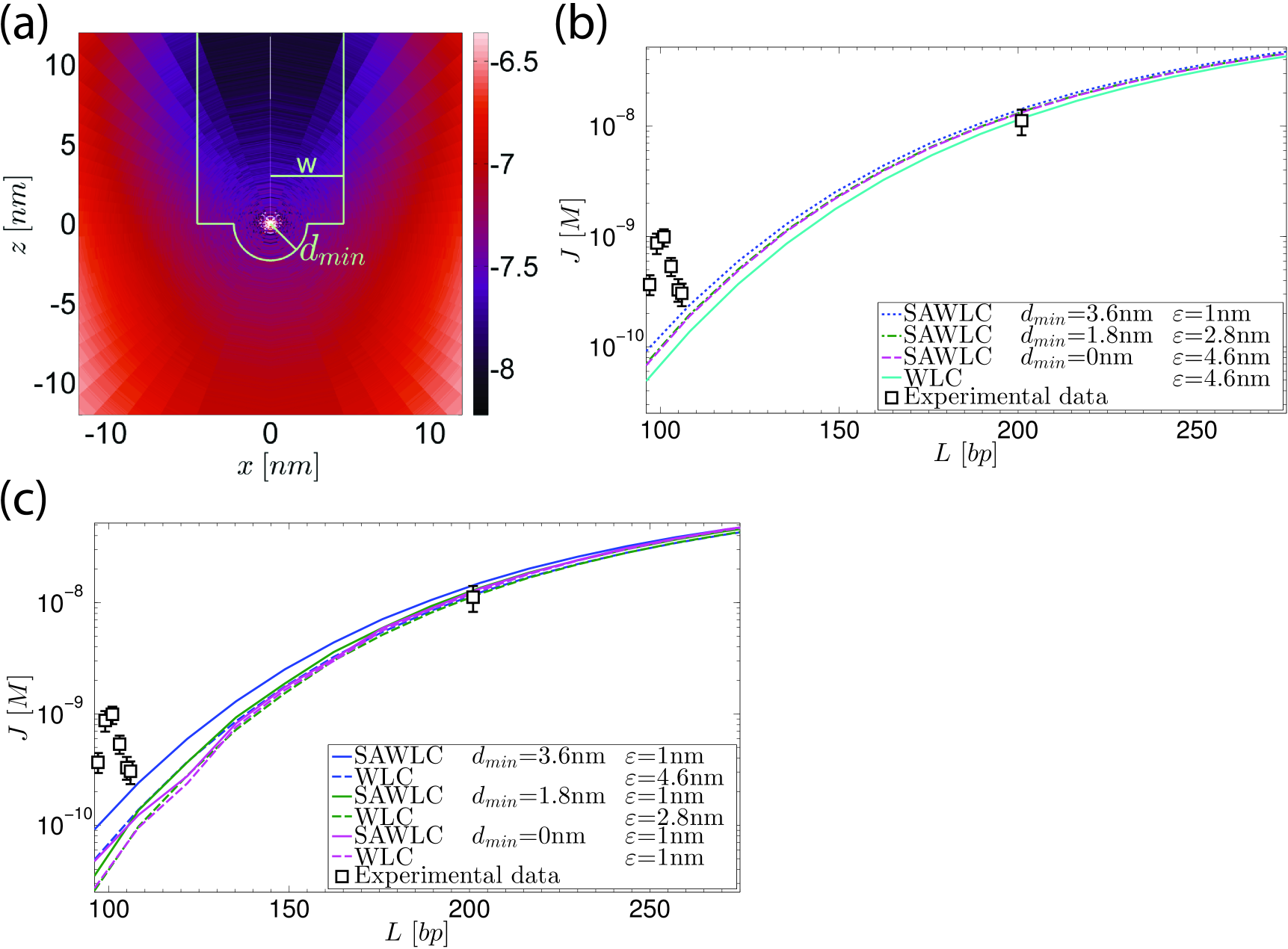
Figure 9: (Color online) Effect of $d_{min}$ on the J-factor in the elastic regime. (a) The volume enclosed in the light-green outline is inaccessible to a SAWLC chain. (b) J-factor for the WLC and SAWLC, varying $d_{min}$, constant $d_{min}+\varepsilon=4.6$ nm. Recent experimental data vafabakhsh_extreme_2012 is shown with black squares. (c) J-factor for the WLC and SAWLC, varying $d_{min}$, constant $\varepsilon=1$ nm. Recent experimental data vafabakhsh_extreme_2012 is shown with black squares. Note, the particular choice of $\mathit{d_{min}+\varepsilon}$ is based on accepted physical values for the effective chain thickness in standard saline conditions. Even though the effects are slightly different in both cases, the magnitude of the effects is less than half an order of magnitude for these values.

V Discussion

We carried out a simulation study of the looping or cyclization J-factor for a self-avoiding worm-like chain (SAWLC) model, taking excluded volume effects into consideration for the first time. The distribution of DNA configurations generated by our numerical algorithm was carefully tested by comparing to scaling theory gennes_scaling_1979 and renormalization group chen_renormalization-group_1992 results for the entropic regime, and indeed faithfully represented the swollen chain partition function. In particular, our algorithm was able to extract the universal exponent $\gamma$ gennes_scaling_1979 , and to reproduce the predicted $N^{-1.92}$ gennes_scaling_1979 ; sinclair_cyclization_1985 J-factor power law for the entropic regime (i.e., where $L\gg l_{p}$). This stronger power-law drop-off is a direct consequence of the self-avoiding assumption, under which the end-to-end separation grows like $\approx N^{0.5876}$ as compared with the ideal chain scaling of $\approx N^{0.5}$. We further showed that the rate of convergence of the SAWLC J-factor power-law exponent to the asymptotic value of $-1.92$ is highly dependent on the semi-flexible chain aspect ratio. This result implies that a highly precise experimental determination of dsDNA aspect ratio can be made by simply measuring this power-law exponent for various looping lengths. Our model and its numerical implementation thus enabled the study of the swollen-chain J-factor in the elastic regime, where swollen-chain analysis to our knowledge has not been carried out previously.

While the statistics in the elastic regime are dominated by elastic energy considerations, our results indicate that the SAWLC model generates a small but detectible effect on the propensity of the chain to loop. Our computations show that in this regime, the angle-independent probability density function of the end-to-end vector $\mathbf{C}\left(\mathbf{r}\right)$ is almost identical for the WLC and SAWLC at points which are accessible to both types of chains. However, there is a range of end-to-end vector $\mathbf{r}$ which is inaccessible to the SAWLC (Fig. 9(a)). The excluded volume of the SAWLC model leads to a redistribution of $\mathbf{C}_{SAWLC}(\mathbf{r})$, as shown in Fig. 9, with the combined weight of the $\mathbf{C}_{WLC}(\mathbf{r})$ within the excluded volume being shifted outside of the SAWLC excluded volume. This could result in an increase in $\int\limits_{\delta\mathbf{r}\,\mathrm{accessible}}\!\!\!\!\!\!\!\!\!\!\!\!\mathbf{C}_{SAWLC}(\mathbf{r})\mbox{d}\mathbf{r}$. Comparison of our numerical calculations of $\mathbf{C}(\mathbf{r})$ for both models (Fig. 9) shows that this redistribution of weight is roughly uniform over the entire range of $\mathbf{r}$. This uniformity is not surprising, since we could have generated the ensemble of short chains using importance sampling (IS, see Appendix  A.1) and then discarded all self-crossing chains, thereby increasing the weight of all allowed chains uniformly. Moreover, if we assume that $\int\limits_{\delta\mathbf{r}\,\mathrm{inaccessible}}\!\!\!\!\!\!\!\!\!\!\!\!\!\!\mathbf{C}_{WLC}(\mathbf{r})\mbox{d}\mathbf{r}$ is redistributed uniformly over the $\mathbf{r}$ range, we obtain a relative increase in the J-factor on the order of $\Delta J/J\approx 10^{-5}$. This is clearly not the main increase in the SAWLC J-factor observed in Fig. 9(b). Instead, the increase that we observe is likely due to the anisotropic nature of $\mathbf{C}(\mathbf{r})$. Namely, the excluded volume for the SAWLC model overlaps the region for which the probability density $\mathbf{C}_{WLC}(\mathbf{r})$ is particularly low (the region enclosed in the light-green outline in Fig. 9(a), in the positive $\hat{z}$ direction). Thus $\mathbf{C}_{WLC}(\mathbf{r})$ averaged over the part of $\delta\mathbf{r}$ accessible to the SAWLC model increases, which in turn leads to an increase in the J-factor (see Eq. 23). Interestingly, the particular choice of the boundary conditions for looping (e.g. minimal bond-to-bond separation) determines the extent of the increase. Consequently, the semi-flexible chain SAWLC J-factor generates the following picture as compared with the WLC J-factor: in the elastic regime, there is a slightly increased probability for looping, while in the entropic regime this trend switches and the SAWLC J-factor falls off with a power law greater than the $-1.5$ value predicted for the WLC.

Previous analysis have shown that the value of the J-factor at the elastic regime can be made very sensitive to boundary conditions and local deformations on the DNA yan_statistics_2005 ; wiggins_exact_2005 ; vafabakhsh_extreme_2012 . Our result adds another possible contribution that, together with the previous explanations, could generate a cumulative effect that might explain the seemingly anomalous bendability effect observed in cyclization experiments cloutier_dna_2005 ; wiggins_high_2006 ; vafabakhsh_extreme_2012 .

Using this insight, what are the experimental implications for looping or cyclization experiments? First, experiments that aim to test looping in the elastic regime will be strongly dependent on boundary conditions. This implies that any observed deviation from a consensus model should first be considered in the context of better models that simulate the effects of the particular boundary conditions. Second, cyclization experiments that are carried out at larger polymer lengths should be considered as the effects of the boundary conditions become negligible for longer polymer contour lengths. In this regime, cyclization measurements can yield accurate estimates for the persistence length of the polymer and effective width or thickness based on measuring the looping probability and comparing to the theoretical predictions shown in Fig. 6. Finally, our model represents a realistic depiction of DNA molecules at length-scales that are relevant to biological regulation. We believe that it can form the basis for a more elaborate model that incorporates protein-DNA interactions.

Appendix A Faithful sampling

A.1 Importance sampling

For the simple (non-self-avoiding) 3D freely-jointed chain (FJC) model, phillips_physical_2009 faithful ensembles of polymer chains can be generated computationally by random step-by-step sampling of the angles of each successive link. In this method, a complete $N$-mer chain is constructed in sequence, where the ith step samples the $\theta_{i},\phi_{i}$ angles to construct an i-mer chain. After sampling a sufficient number of chains, the partition function can be evaluated from the $N_{c}$ sampled chains as follows:

$$Z_{N}=\sum_{j=1}^{N_{c}}e^{-\beta E_{j}}=N_{c},$$ (49)

where $E_{j}=0$ in the FJC case. Any physical property $\left\langle f\right\rangle$ can be likewise computed:

$$\left\langle f\right\rangle=\frac{\sum\limits_{j=1}^{N_{c}}f\left(\left\{\theta_{N},\phi_{N}\right\}_{j}\right)e^{-\beta E_{j}}}{\sum\limits_{j=1}^{N_{c}}e^{-\beta E_{j}}}=\frac{\sum\limits_{j=1}^{N_{c}}f\left(\left\{\theta_{N},\phi_{N}\right\}_{j}\right)}{N_{c}}.$$ (50)

When trying to collect an ensemble of plausible polymer configurations for the WLC model, the simple sampling algorithm described above is insufficient. Unlike the FJC model, in the WLC model link orientations depend strongly on the elastic energy of bending (see Eq. 2). Namely, sharp bends are highly improbable as compared to small perturbations away from the non-bending minima. As a result, a uniform sampling procedure of the relative link orientations will yield a disproportionate number of improbable chains that are characterized by very large bending energies, which will increase by orders of magnitude the computation time necessary to obtain a statistically significant and representative ensemble.

In order to alleviate this problem, and generate a faithful sampling algorithm for the WLC model (i.e. $E^{hw}=0$), we employ a sampling method termed importance sampling (IS) grassberger_pruned-enriched_1997 . In IS we assign the following Boltzmann weight to the $i$th link:

$$\exp\left[-\beta E^{el}\left(\theta_{i},\phi_{i}\right)\right].$$ (51)

We then sample the chain links according to the following probability distribution:

$$p^{el}\left(\theta_{i},\phi_{i}\right)=\frac{\exp\left[-\beta E^{el}\left(\theta_{i},\phi_{i}\right)\right]}{\int\limits_{-1}^{1}\mbox{d}\cos\theta_{i}\int\limits_{0}^{2\pi}\mbox{d}\phi_{i}\exp\left[-\beta E^{el}\left(\theta_{i},\phi_{i}\right)\right]}.$$ (52)

As a result, the orientation angles that are more likely to occur due to low bending energies will be chosen more frequently, thus reflecting faithfully the underlying distribution. Furthermore, since each sampled link appears in a chain of $N$ sampled links, the cumulative probability to obtain each chain is a product of the individual link probabilities sampled at every stage of the chain construction, as follows:

$$P_{tot}^{el}\left(\left\{\theta_{N},\phi_{N}\right\}\right) \equiv \prod_{i=2}^{N}p^{el}\left(\theta_{i},\phi_{i}\right)=\prod_{i=2}^{N}\frac{\exp\left[-\beta E^{el}\left(\theta_{i},\phi_{i}\right)\right]}{\int\limits_{-1}^{1}\mbox{d}\cos\theta_{i}\int\limits_{0}^{2\pi}\mbox{d}\phi_{i}\exp\left[-\beta E^{el}\left(\theta_{i},\phi_{i}\right)\right]}$$

$$= \frac{\exp\left[-\beta\sum\limits_{i=2}^{N}E^{el}\left(\theta_{i},\phi_{i}\right)\right]}{\int\limits_{-1}^{1}\mbox{d}\cos\theta_{1}\int\limits_{0}^{2\pi}\mbox{d}\phi_{1}\cdots\int\limits_{-1}^{1}\mbox{d}\cos\theta_{N}\int\limits_{0}^{2\pi}\mbox{d}\phi_{N}\exp\left[-\underset{i}{\sum}\beta E^{el}\left(\theta_{i},\phi_{i}\right)\right]}=\frac{\exp\left[-\beta E_{chain}\right]}{\int\limits_{all~{}configurations}\exp\left[-\beta E_{chain}\right]}.$$

Thus, this method generates complete WLC chains according to their statistical probabilities in the ensemble.
According to statistics theory,fristedt_modern_1996 if $X\,:\,\Omega\rightarrow\mathbb{R}$ is a random variable in some probability space $\left(\Omega,\mathcal{F},P\right)$ and one wishes to estimate the expected value of $X$ under $P$, provided that one has random samples $x_{1},...,\,x_{n}$ generated according to $P$, then an empirical estimate of $\mbox{E}[X;P]$ is

$$\hat{\mbox{E}}_{n}[X;P]=\frac{1}{n}\sum_{i=1}^{n}x_{i}.$$ (54)

This simplifies the computation of any physical observable$\left\langle f\right\rangle$ for the IS to:

$$\left\langle f\right\rangle=\frac{1}{N_{c}}\sum\limits_{j=1}^{N_{c}}f\left(\left\{\theta_{N},\phi_{N}\right\}_{j}\right).$$ (55)

A.2 Weighted-biased sampling

The IS method can be used to generate chains for the SAWLC model by following (52) and then discarding chains with overlapping links. However, this method is extremely inefficient and leads to extreme sampling attrition sadanobu_continuous_1997 .

Naively one could replace Eq. (52) with

$$p_{i}\left(\left\{\theta_{i},\phi_{i}\right\}\right)=\\ \frac{\exp\left[-\beta E^{el}\left(\theta_{i},\phi_{i}\right)\right]\Theta_{i}^{hw}\left(\left\{\theta_{i},\phi_{i}\right\}\right)}{\int\limits_{-1}^{1}\mbox{d}\cos\theta_{i}\int\limits_{0}^{2\pi}\mbox{d}\phi_{i}\exp\left[-\beta E^{el}\left(\theta_{i},\phi_{i}\right)\right]\Theta_{i}^{hw}\left(\left\{\theta_{i},\phi_{i}\right\}\right)},$$ (56)

where $\Theta_{i}^{hw}\left(\left\{\theta_{i},\phi_{i}\right\}\right)$ was defined previously in Eq. (7), and follow the same (IS) procedure. However, since the hard-wall potential eliminates a certain percentage of the possible configurations, a misrepresentation of the sampled chains in the ensemble results, as discussed in rosenbluth_monte_1955 . Therefore, in order to produce a faithful representation of the partition function, each generated chain has to be assigned with a weight for the excluded volume case.

In order to gain insight into the calculation of these weights and their necessity, we consider the general case of self-avoiding chains. We denote the probability of a chain $j$ with $N$ links to appear in a statistical ensemble as $P_{j}^{S}$:

$$P_{j}^{S}=\frac{e^{-\beta E_{j}}}{Z_{N}^{S}},$$ (57)

where $Z_{N}^{S}$ is the partition function of the statistical ensemble. We denote the probability of a chain $j$ with $N$ links to be generated with IS as $P_{j}^{IS}$. Due to the way the chain links are sampled:

$$P_{j}^{IS}=\prod_{i=2}^{N}p_{i}\left(\left\{\theta_{i},\phi_{i}\right\}_{j}\right) = \prod_{i=2}^{N}\left(\frac{\exp\left[-\beta E^{el}\left(\theta_{i},\phi_{i}\right)\right]\Theta_{i}^{hw}\left(\left\{\theta_{i},\phi_{i}\right\}_{j}\right)}{\int\limits_{-1}^{1}\mbox{d}\cos\theta_{i}\int\limits_{0}^{2\pi}\mbox{d}\phi_{i}\exp\left[-\beta E^{el}\left(\theta_{i},\phi_{i}\right)\right]\Theta_{i}^{hw}\left(\left\{\theta_{i},\phi_{i}\right\}_{j}\right)}\right)$$ (58)

$$= \frac{e^{-\beta E_{j}}}{\prod_{i=2}^{N}\left(\int\limits_{-1}^{1}\mbox{d}\cos\theta_{i}\int\limits_{0}^{2\pi}\mbox{d}\phi_{i}\exp\left[-\beta E^{el}\left(\theta_{i},\phi_{i}\right)\right]\Theta_{i}^{hw}\left(\left\{\theta_{i},\phi_{i}\right\}_{j}\right)\right)}\,.$$

While the numerators in (58) and (57) agree, the denominators differ. Furthermore, the denominator in (58) is different for each chain configuration, unlike the denominator in (57). Thus, to remove the bias for chain $j$, it is sufficient to take the denominator of (58) as the counter-weight $W\left(\left\{\theta_{N},\phi_{N}\right\}\right)$:

$$W\left(\left\{\theta_{N},\phi_{N}\right\}\right)=\\ \prod_{i=2}^{N}\int\limits_{-1}^{1}\!\!\mbox{d}\cos\theta_{i}\int\limits_{0}^{2\pi}\!\!\mbox{d}\phi_{i}\exp\left[-\beta E^{el}\left(\theta_{i},\phi_{i}\right)\right]\Theta_{i}^{hw}\left(\left\{\theta_{i},\phi_{i}\right\}\right),$$ (59)

which allows to define the link-by-link counter-weight as

$$\omega_{i}\left(\left\{\theta_{i},\phi_{i}\right\}\right)=\\ \int\limits_{-1}^{1}\mbox{d}\cos\theta_{i}\int\limits_{0}^{2\pi}\mbox{d}\phi_{i}\exp\left[-\beta E^{el}\left(\theta_{i},\phi_{i}\right)\right]\Theta_{i}^{hw}\left(\left\{\theta_{i},\phi_{i}\right\}\right)=\\ \int\limits_{non-colliding\,directions}\mbox{d}\theta_{i}\mbox{d}\phi_{i}\exp\left[-\beta E^{el}\left(\theta_{i},\phi_{i}\right)\right],$$ (60)

and the Rosenbluth factor as

$$W\left(\left\{\theta_{N},\phi_{N}\right\}\right)=\prod_{i=1}^{N}\omega_{i}\left(\left\{\theta_{i},\phi_{i}\right\}\right).$$ (61)

The partition function takes on the following form in the WBS case:

$$Z_{N}=\sum_{j=1}^{N_{c}}W\left(\left\{\theta_{N},\phi_{N}\right\}_{j}\right),$$ (62)

and the average value $\left\langle f\right\rangle$ of a physical property is calculated as:

$$\left\langle f\right\rangle=\frac{\sum\limits_{j=1}^{N_{c}}f\left(\left\{\theta_{N},\phi_{N}\right\}_{j}\right)W\left(\left\{\theta_{N},\phi_{N}\right\}_{j}\right)}{\sum\limits_{j=1}^{N_{c}}W\left(\left\{\theta_{N},\phi_{N}\right\}_{j}\right)}.$$ (63)

Appendix B Additional computations

B.1 Computation of power-law exponents

To compute the power-law exponents $\nu$ of $\sqrt{\left\langle R^{2}\right\rangle}$ and $\chi$ of the J-factor in Sections IV.1 and IV.2, respectively, we started off by taking a logarithm of both the data and $L/b$. The power-law exponent could then theoretically be read from the slope of the logarithm of the data as a function of $\mbox{log}\left(L/b\right)$. The data, however, are very sensitive to noise in the sampled data. Thus, we employed a smoothing algorithm to deduce the slope of the data at each point: We used a sliding window along the values of $L/b$. The range of the plot covered by the sliding window was fitted to a linear function, and the slope of the linear function was taken as the slope of the plot at the center of the sliding window. The size of the sliding window was increased as $L/b$ increased in order to account for increased noise at greater values of $L/b$.

B.2 A scaling theory derivation for the asymptotic power law for looping in the swollen coil regime

The WLC model predicts that the J-factor will scale like $\mathit{N^{-\frac{3}{2}}}$ in the entropic regime, when the length of the polymer is much longer than the persistence length ($\mathit{N\gg l_{p}}$) phillips_physical_2009 . Likewise, the swollen chain also exhibits some power-law dependency in the entropic regime. The asymptotic behavior of the SAWLC model in the entropic regime can be inferred from the existing theory for a freely-jointed chain on a 3D lattice. In the following derivation we rely on the arguments given in des_cloizeaux_lagrangian_1974 ; gennes_scaling_1979 . We first assume that in the entropic regime, the probability of looping scales as:

$$p_{loop}\left(N\right)\propto N^{-\alpha}.$$ (64)

Since the probability for looping is defined as ratio of the number of looped polymer configurations to the total number of polymer configurations, we begin with the asymptotic expression for the total number of available configurations for a self-avoiding chain of $N$ links mckenzie_polymers_1976 :

$$Z=\widetilde{z}^{N}N^{\gamma-1},$$ (65)

where $\widetilde{z}$ is a number corresponding to the effective lattice space that the chain is defined on (i.e. $\widetilde{z}=6$ for an ideal chain defined on a cubic lattice). Next, the mean square end-to-end distance for a swollen chain follows a scaling law, originally derived by Flory flory_statistical_1969 :

$$R_{f}\propto N^{\nu}.$$ (66)

Combining these two results, it is possible to derive an expression for the total number of looped states for a self-avoiding random-walk chain. This result is derived for a grid with pixels of size $a$, such that a loop is formed when the two ends are separated by a distance $a$. Thus, on a grid, a self-avoiding random-walk chain will form a closed polygon of $N+1$ edges, which implies gennes_scaling_1979

$$Z_{loop}\propto\widetilde{z}^{N}\left(\frac{a}{R_{f}}\right)^{3},$$ (67)

with a normalizing term which takes into account that the loop can be closed anywhere within a sphere of radius which is roughly equal to the Flory radius . Given this expression, we can now write the expression for the probability for looping in the asymptotic regime gennes_scaling_1979 :

$$p_{loop}\left(N\right)\equiv\frac{1}{a^{3}}\frac{Z_{loop}}{Z}\propto\frac{1}{R_{f}^{3}\,N^{\gamma-1}}\propto N^{-\left(3\nu+\gamma-1\right)},$$ (68)

which is the desired power law. Finally, using the RG derived values for $\nu=0.5876$ and $\gamma=1.1568\simeq 7/6,$ caracciolo_high-precision_1998 ; clisby_self-avoiding_2007 ; clisby_accurate_2010 we obtain

$$\chi=3\nu+\gamma-1=1.9196\,.$$ (69)

The universal nature of exponent $\gamma$ implies that the J-factor power law for semi-flexible swollen chains ($\frac{w}{b}<1$) can be predicted simply from the end-to-end exponent $\nu$.

References

- [1] Homer Jacobson and Walter H. Stockmayer. Intramolecular reaction in polycondensations. i. the theory of linear systems. The Journal of Chemical Physics, 18(12):1600–1606, 1950.
- [2] Paul J. Flory. Statistical mechanics of chain molecules. Interscience Publishers, 1969.
- [3] Donald M. Crothers, Jacqueline Drak, Jason D. Kahn, and Stephen D. Levene. DNA bending, flexibility, and helical repeat by cyclization kinetics. In James E. Dahlberg David M.J. Lilley, editor, Methods in Enzymology, volume Volume 212 of DNA Structures Part B: Chemical and Electrophoretic Analysis of DNA, pages 3–29. Academic Press, 1992.
- [4] T. E. Cloutier and J. Widom. DNA twisting flexibility and the formation of sharply looped protein-DNA complexes. Proceedings of the National Academy of Sciences, 102(10):3645–3650, February 2005.
- [5] John F. Marko and Eric D. Siggia. Stretching DNA. Macromolecules, 28(26):8759–8770, December 1995.
- [6] Paul A. Wiggins, Thijn van der Heijden, Fernando Moreno-Herrero, Andrew Spakowitz, Rob Phillips, Jonathan Widom, Cees Dekker, and Philip C. Nelson. High flexibility of DNA on short length scales probed by atomic force microscopy. Nature Nanotechnology, 1(2):137–141, November 2006.
- [7] Reza Vafabakhsh and Taekjip Ha. Extreme bendability of DNA less than 100 base pairs long revealed by single-molecule cyclization. Science, 337(6098):1097–1101, August 2012.
- [8] Pierre-Gilles Gennes. Scaling Concepts in Polymer Physics. Cornell University Press, Ithaca, NY, November 1979.
- [9] Zheng Yu Chen and Jaan Noolandi. Renormalization-group scaling theory for flexible and wormlike polymer chains. The Journal of Chemical Physics, 96(2):1540–1548, January 1992.
- [10] Manish Nepal, Alon Yaniv, Eyal Shafran, and Oleg Krichevsky. Structure of DNA coils in dilute and semidilute solutions. Physical Review Letters, 110(5):058102, January 2013.
- [11] V. V. Rybenkov, N. R. Cozzarelli, and A. V. Vologodskii. Probability of DNA knotting and the effective diameter of the DNA double helix. Proceedings of the National Academy of Sciences, 90(11):5307–5311, June 1993.
- [12] Douglas R. Tree, Abhiram Muralidhar, Patrick S. Doyle, and Kevin D. Dorfman. Is DNA a good model polymer? Macromolecules, 46(20):8369–8382, October 2013.
- [13] P. J. Flory and J. A. Semlyen. Macrocyclization equilibrium constants and the statistical configuration of poly(dimethylsiloxane) chains. Journal of the American Chemical Society, 88(14):3209–3212, July 1966.
- [14] Hiromi Yamakawa. Modern Theory of Polymer Solutions. 1971.
- [15] Roee Amit, Hernan G. Garcia, Rob Phillips, and Scott E. Fraser. Building enhancers from the ground up: A synthetic biology approach. Cell, 146(1):105–118, July 2011.
- [16] Jie Yan, Ryo Kawamura, and John F. Marko. Statistics of loop formation along double helix DNAs. Physical Review E, 71(6):061905, June 2005.
- [17] Paul A. Wiggins, Rob Phillips, and Philip C. Nelson. Exact theory of kinkable elastic polymers. Physical Review E, 71(2):021909, February 2005.
- [18] Paul A Wiggins and Philip C Nelson. Generalized theory of semiflexible polymers. Physical review. E, Statistical, nonlinear, and soft matter physics, 73(3 Pt 1):031906, March 2006.
- [19] Andrew M. Sinclair, Mitchell A. Winnik, and Gerard Beinert. Cyclization dynamics of polymers. 18. capture radius effects in the end-to-end cyclization rate of polymers. Journal of the American Chemical Society, 107(20):5798–5800, October 1985.
- [20] O. Kratky, G. Porod. Röntgenuntersuchung gelöster fadenmoleküle. Rec. Trav. Chim. Pays-Bas., 68:1106–1123, 1949.
- [21] P. J. Flory, U. W. Suter, and M. Mutter. Macrocyclization equilibriums. 1. theory. Journal of the American Chemical Society, 98(19):5733–5739, September 1976.
- [22] E. R. Semlyen. Cyclic Polymers. Springer, Dordrecht ; Boston, 2nd ed. 2000 edition edition, August 2000.
- [23] Nathan Clisby. Accurate estimate of the critical exponent for self-avoiding walks via a fast implementation of the pivot algorithm. Physical Review Letters, 104(5):055702, February 2010.
- [24] Luc Devroye. Non-uniform random variate generation. Springer-Verlag, New York, 1986.
- [25] Wilhelm M. Pieper. Recursive gauss integration. Communications in Numerical Methods in Engineering, 15(2):77–90, 1999.
- [26] Juan J. De Pablo and Fernando A. Escobedo. Monte Carlo methods for polymeric systems. In I. Prigogine and Stuart A. Rice, editors, Advances in Chemical Physics, volume 105, pages 337–367. John Wiley & Sons, Inc., Hoboken, NJ, USA, 1998.
- [27] Marshall N. Rosenbluth and Arianna W. Rosenbluth. Monte Carlo calculation of the average extension of molecular chains. The Journal of Chemical Physics, 23(2):356–359, February 1955.
- [28] Rob Phillips, Jané Kondev, and Julie Theriot. Physical Biology of the Cell. New York: Garland Science, 2009.
- [29] Peter Grassberger. Pruned-enriched rosenbluth method: Simulations of polymers of chain length up to 1 000 000. Physical Review E, 56(3):3682–3693, September 1997.
- [30] Bert E. Fristedt and Lawrence F. Gray. A Modern Approach to Probability Theory. Birkhauser, 1996 edition edition, December 1996.
- [31] Jiro Sadanobu and William A. Goddard III. The continuous configurational boltzmann biased direct Monte Carlo method for free energy properties of polymer chains. The Journal of Chemical Physics, 106(16):6722–6729, April 1997.
- [32] J. des Cloizeaux. Lagrangian theory for a self-avoiding random chain. Physical Review A, 10(5):1665–1669, November 1974.
- [33] D. S. McKenzie. Polymers and scaling. Physics Reports, 27(2):35–88, September 1976.
- [34] Sergio Caracciolo, Maria Serena Causo, and Andrea Pelissetto. High-precision determination of the critical exponent for self-avoiding walks. Physical Review E, 57(2):R1215–R1218, February 1998.
- [35] Nathan Clisby, Richard Liang, and Gordon Slade. Self-avoiding walk enumeration via the lace expansion. Journal of Physics A: Mathematical and Theoretical, 40(36):10973–11017, 2007.