High-order Compact Difference Schemes for the Modified Anomalous Subdiffusion Equation.

Abstract

In this paper, two kinds of high-order compact finite difference schemes for second-order derivative are developed. Then a second-order numerical scheme for a Riemann-Liouvile derivative is established based on a fractional centered difference operator. We apply these methods to a fractional anomalous subdiffusion equation to construct two kinds of novel numerical schemes. The solvability, stability and convergence analysis of these difference schemes are studied by using Fourier method. The convergence orders of these numerical schemes are $\mathcal{O}(\tau^{2}+h^{6})$ and $\mathcal{O}(\tau^{2}+h^{8})$, respectively. Finally, numerical experiments are displayed which are in line with the theoretical analysis.

Key words: Modified anomalous subdiffusion equation; High-order compact difference schemes; Fourier method; Riemann-Liouville derivative; Grünwald-Letnikov derivative

1 Introduction

The phenomenological diffusion equation can be derived by the following Fick’s first law [1] (which describes steady-state diffusion),

$$\begin{array}[]{lll}\displaystyle\mathcal{J}=-\kappa\nabla u.\end{array}$$

Combing the following conservation law of energy

$$\begin{array}[]{lll}\displaystyle\frac{\partial u}{\partial t}=-\nabla\cdot\mathcal{J},\end{array}$$

one can obtain the diffusion equation below (also known as Fick’s second law or the heat equation)

$$\begin{array}[]{lll}\displaystyle\frac{\partial u}{\partial t}=\nabla\cdot(\kappa\nabla u).\end{array}$$

This equation well characterizes the classic diffusion phenomenon [2].

However, if the diffusion is abnormal, that is to say, it follows non-Gaussian statistics or can be interpreted as the Lévy stable densities, then the above equation can not well describe such anomalous diffusion. Generally speaking, the fractional differential equations can well describe and model these anomalous diffusion phenomena [3]. The corresponding fractional Fick’s law has been proposed [4].

$$\begin{array}[]{lll}\displaystyle\mathcal{J}_{\mathcal{A}}=-\mathcal{A}\cdot\,_{RL}D_{0,t}^{1-\alpha}\nabla u,\;\alpha\in(0,1).\end{array}$$

Combination of this equation with equation (2) gives

$$\begin{array}[]{lll}\displaystyle\frac{\partial u}{\partial t}=\mathcal{A}\cdot\,_{RL}D_{0,t}^{1-\alpha}\frac{\partial^{2}u}{\partial x^{2}},\end{array}$$

where $0<\alpha<1$, and $\mathcal{A}>0$ is the anomalous diffusion coefficient. If $\alpha=1$, it is just the normal diffusion equation. Here $\,{}_{RL}D_{0,t}^{1-\alpha}$ is the Riemann-Liouville operator, which is defined as follows:

$$\begin{array}[]{ll}\,{}_{RL}D_{0,t}^{1-\alpha}u(x,t)=\frac{1}{\Gamma(\alpha)}\frac{\partial}{\partial t}\int_{0}^{t}\frac{u(x,s)}{(t-s)^{1-\alpha}}ds,\end{array}$$

where $\Gamma(\cdot)$ is the Gamma function.

Recently, a modified fractional Fick’s law has been used to describe processes that become less anomalous as time progresses by the inclusion of a secondary fractional time derivative acting on a diffusion operator [5],

$$\begin{array}[]{lll}\displaystyle\mathcal{J}_{\mathcal{A,B}}=-\left(\mathcal{A}\cdot\,_{RL}D_{0,t}^{1-\alpha}+\mathcal{B}\cdot\,_{RL}D_{0,t}^{1-\beta}\right)\nabla u,\end{array}$$

where $0<\alpha<1,0<\beta<1$, and $\mathcal{A}>0,\mathcal{B}>0$ are the anomalous diffusion coefficients. Thus, the modified fractional anomalous diffusion equation is obtained [6],

$$\begin{array}[]{lll}\displaystyle\frac{\partial{{}u(x,t)}}{\partial{t}}=\left(\mathcal{A}\cdot\,_{RL}D_{0,t}^{1-\alpha}+\mathcal{B}\cdot\,_{RL}D_{0,t}^{1-\beta}\right)\left[\frac{\partial^{2}u(x,t)}{\partial{x^{2}}}\right].\end{array}$$

Till now, various kinds of anomalous diffusion equations have been studied numerically, see [7, 8, 9, 10, 11, 12, 13, 14, 15, 16, 17] and many the references cited therein. However, it seems that only a few numerical studies are available for the two-term subdiffusions of the above form.

In the present paper, we aim to study the following modified anomalous diffusion equation with a source term

$$\begin{array}[]{lll}\displaystyle\frac{\partial{{}u(x,t)}}{\partial{t}}=\left(\mathcal{A}\cdot\,_{RL}D_{0,t}^{1-\alpha}+\mathcal{B}\cdot\,_{RL}D_{0,t}^{1-\beta}\right)\left[\frac{\partial^{2}u(x,t)}{\partial{x^{2}}}\right]+f(x,t),\;\;\;0<x<L,\;\;\;0<t\leq T$$,\end{array}$$

subject to the initial and Dirichlet boundary value conditions

$$\begin{array}[]{ll}u(x,0)=\phi(x),\;\;0<x<L,\end{array}$$

$$\begin{array}[]{ll}u(0,t)=\varphi_{{}_{1}}(t),\;\;0\leq t\leq T,\end{array}$$

$$\begin{array}[]{ll}u(L,t)=\varphi_{{}_{2}}(t),\;\;0\leq t\leq T,\end{array}$$

where $f(x,t)$, $\phi(x)$, $\varphi_{{}_{1}}(t)$ and $\varphi_{{}_{2}}(t)$ are suitably smooth.

Jiang and Chen proposed a collocation method based on reproducing kernels to solve a modified anomalous subdiffusion equation (3) with a linear source term on a finite domain [18]. In [19], Liu et al., constructed a conditionally stable difference scheme for equation (3) with a nonlinear source term, and they proved that the convergence order is $\mathcal{O}(\tau+h^{2})$ by the energy method. In [20], Mohebbi et al. considered an unconditionally stable difference scheme of order $\mathcal{O}(\tau+h^{4})$. Wang and Vong [21] presented a compact method for the numerical simulation of the modified anomalous subdiffusion equation (3), and they achieved the convergence order $\mathcal{O}(\tau^{2}+h^{4})$. The aim of this paper is to propose much higher order numerical methods for equation (3). We construct two kinds of high-order compact difference schemes and provide a detailed study of the stability and convergence of the proposed methods by using the Fourier method. We demonstrate that the convergence orders are $\mathcal{O}(\tau^{2}+h^{6})$ and $\mathcal{O}(\tau^{2}+h^{8})$, respectively. One of advantages of compact difference schemes are that they can produce highly accurate numerical solutions but involves the less number of grid points. Thus, compact schemes result in matrices that have smaller band-width compared with non-compact schemes. For example, a sixth-order finite difference scheme involves seven grid points, while sixth-order compact difference scheme only needs five grid points. Another additional advantage of the compact high order methods is that the methods described here leads to diagonal linear systems, thus allowing the use of fast diagonal solvers. Different from the typical differential equations, even if we use the lower order methods for solving the fractional differential equations, we still need more calculations and strong spaces. If we use the higher order methods for fractional differential equations, the calculations and memory capacities can not remarkably increase. In this sense, the higher order numerical methods for fractional calculus and fractional differential equations attract more and more interest.

The rest of this article is organized as follows. In Section 2, we firstly develop a sixth-order and an eight-order difference scheme for second-order derivative, next a second-order numerical scheme for the Riemann-Liouville derivative is proposed. Applications of these methods to equation (3) give two effective finite difference schemes. The solvability, stability and convergence of the numerical methods are discussed in Sections 3, 4 and 5, respectively. The numerical experiments are performed for equation (3) with the methods developed in this paper are given in Section 6, which support the theoretical analysis. Finally, concluding remarks are drawn in the last section.

2 Numerical Schemes

Let $t_{k}=k\tau~{}(k=0,1,\cdots,N)$ and $x_{j}=jh~{}(j=0,1,\cdots,M),$ where the grid sizes in time and space are defined by $\tau=T/N$ and $h=L/M$, respectively.

Define the following centered difference operator as

$$\begin{array}[]{lll}\displaystyle\delta_{x}u(x_{j},t_{k})=u(x_{j+\frac{1}{2}},t_{k})-u(x_{j-\frac{1}{2}},t_{k}),\end{array}$$

then we have

$$\begin{array}[]{lll}\displaystyle\delta_{x}^{2}u(x_{j},t_{k})=u(x_{j+1},t_{k})-2u(x_{j},t_{k})+u(x_{j-1},t_{k}).\end{array}$$

It is well known that a second-order approximation for the derivative $\frac{\partial^{2}u(x_{j},t_{k})}{\partial{x^{2}}}$ is given by the following second-order centered difference scheme

$$\begin{array}[]{rrr}\displaystyle\frac{\partial^{2}u(x_{j},t_{k})}{\partial{x^{2}}}=\frac{\delta_{x}^{2}u(x_{j},t_{k})}{h^{2}}+\mathcal{O}(h^{2}).\end{array}$$

A fourth-order compact difference scheme has also been constructed [22],

$$\begin{array}[]{rrr}\displaystyle\frac{\partial^{2}u(x_{j},t_{k})}{\partial{x^{2}}}=\frac{1}{h^{2}}\left(1+\frac{1}{12}\delta_{x}^{2}\right)^{-1}\par\par\delta_{x}^{2}u(x_{j},t_{k})+\mathcal{O}(h^{4}).\end{array}$$

Next, we develop two high-order compact difference schemes for the second-order spatial derivative by the following lemma.

Lemma 1. Define the following two operators:

$$\begin{array}[]{lll}\displaystyle\mathscr{L}_{1}=:\frac{1}{h^{2}}\left(1-\frac{1}{90}\delta_{x}^{4}\right)^{-1}\delta_{x}^{2}\left(1-\frac{1}{12}\delta_{x}^{2}\right),\end{array}$$

and

$$\begin{array}[]{lll}\displaystyle\mathscr{L}_{2}=:\frac{1}{h^{2}}\left(1+\frac{1}{560}\delta_{x}^{6}\right)^{-1}\delta_{x}^{2}\left(1-\frac{1}{12}\delta_{x}^{2}+\frac{1}{90}\delta_{x}^{4}\right),\end{array}$$

then

$$\begin{array}[]{lll}\displaystyle\frac{\partial^{2}u(x_{j},t_{k})}{\partial{x^{2}}}=\mathscr{L}_{1}u(x_{j},t_{k})+\mathcal{O}(h^{6})\end{array}$$

and

$$\begin{array}[]{lll}\displaystyle\frac{\partial^{2}u(x_{j},t_{k})}{\partial{x^{2}}}=\mathscr{L}_{2}u(x_{j},t_{k})+\mathcal{O}(h^{8})\end{array}$$

hold.

Proof. In view of the following approximation scheme [23]

$$\begin{array}[]{lll}\displaystyle\frac{\partial^{2}u(x_{j},t_{k})}{\partial{x^{2}}}&=&\displaystyle\left[\frac{2}{h}\sinh^{-1}\left(\frac{\delta_{x}}{2}\right)\right]^{2}u(x_{j},t_{k})\vspace{0.2 cm}\\ &=&\displaystyle\frac{1}{h^{2}}\left[\delta_{x}-\frac{1}{24}\delta_{x}^{3}+\frac{3}{640}\delta_{x}^{5}-\frac{5}{7168}\delta_{x}^{7}+\cdots\right]^{2}u(x_{j},t_{k})\vspace{0.2 cm}\\ &=&\displaystyle\frac{1}{h^{2}}\left[\delta_{x}^{2}-\frac{1}{12}\delta_{x}^{4}+\frac{1}{90}\delta_{x}^{6}-\frac{1}{560}\delta_{x}^{8}+\frac{1}{3150}\delta_{x}^{10}-\frac{1}{16632}\delta_{x}^{12}+\cdots\right]u(x_{j},t_{k}),\end{array}$$

then one obtains

$$\begin{array}[]{lll}&\displaystyle\frac{1}{h^{2}}\left(1-\frac{1}{90}\delta_{x}^{4}\right)^{-1}\delta_{x}^{2}\left(1-\frac{1}{12}\delta_{x}^{2}\right)u(x_{j},t_{k})\vspace{0.3 cm}\\ &=\displaystyle\frac{1}{h^{2}}\left[\delta_{x}^{2}-\frac{1}{12}\delta_{x}^{4}+\frac{1}{90}\delta_{x}^{6}-\frac{1}{1080}\delta_{x}^{8}+\cdots\right]u(x_{j},t_{k})\vspace{0.2 cm}\\ &=\displaystyle\frac{\partial^{2}u(x_{j},t_{k})}{\partial{x^{2}}}+\frac{13}{15120h^{2}}\delta_{x}^{8}u(x_{j},t_{k})+\mathcal{O}(h^{8})\vspace{0.2 cm}\\ &=\displaystyle\frac{\partial^{2}u(x_{j},t_{k})}{\partial{x^{2}}}+\frac{13h^{6}}{15120}\frac{\partial^{8}u(x_{j},t_{k})}{\partial{x^{8}}}+\mathcal{O}(h^{8})\end{array}$$

and

$$\begin{array}[]{lll}\displaystyle&\displaystyle\frac{1}{h^{2}}\left(1+\frac{1}{560}\delta_{x}^{6}\right)^{-1}\delta_{x}^{2}\left(1-\frac{1}{12}\delta_{x}^{2}+\frac{1}{90}\delta_{x}^{4}\right)u(x_{j},t_{k})\vspace{0.3cm}\\ &=\displaystyle\frac{1}{h^{2}}\left[\delta_{x}^{2}-\frac{1}{12}\delta_{x}^{4}+\frac{1}{90}\delta_{x}^{6}-\frac{1}{560}\delta_{x}^{8}+\frac{1}{6720}\delta_{x}^{10}+\cdots\right]u(x_{j},t_{k})\vspace{0.2 cm}\\ &=\displaystyle\frac{\partial^{2}u(x_{j},t_{k})}{\partial{x^{2}}}+\frac{197}{28672000h^{2}}\delta_{x}^{10}u(x_{j},t_{k})+\mathcal{O}(h^{10})\vspace{0.2 cm}\\ &=\displaystyle\frac{\partial^{2}u(x_{j},t_{k})}{\partial{x^{2}}}+\frac{197h^{8}}{28672000}\frac{\partial^{10}u(x_{j},t_{k})}{\partial{x^{10}}}+\mathcal{O}(h^{10}).\end{array}$$

That is,

$$\begin{array}[]{lll}\displaystyle\frac{\partial^{2}u(x_{j},t_{k})}{\partial{x^{2}}}=\frac{1}{h^{2}}\left(1-\frac{1}{90}\delta_{x}^{4}\right)^{-1}\delta_{x}^{2}\left(1-\frac{1}{12}\delta_{x}^{2}\right)u(x_{j},t_{k})+\mathcal{O}(h^{6}),\end{array}$$

and

$$\begin{array}[]{lll}\displaystyle\frac{\partial^{2}u(x_{j},t_{k})}{\partial{x^{2}}}=\frac{1}{h^{2}}\left(1+\frac{1}{560}\delta_{x}^{6}\right)^{-1}\delta_{x}^{2}\left(1-\frac{1}{12}\delta_{x}^{2}+\frac{1}{90}\delta_{x}^{4}\right)u(x_{j},t_{k})+\mathcal{O}(h^{8}).\end{array}$$

This completes the proof.   

Lemma 2 [24] For the suitably smooth function $u(x,t)$ with respect to $x$, arbitrary different numbers $p$, $q$ and $s$, one has

$$u(x,t_{s})=\frac{(t_{s}-t_{q})u(x,t_{p})+(t_{p}-t_{s})u(x,t_{q})}{t_{p}-t_{q}}+\mathcal{O}\left(\left|(t_{p}-t_{s})(t_{q}-t_{s})\right|\right).$$

Next, we develop a second order numerical scheme for the Riemann-Liouvile derivative at nongrid points $\left(x_{j},t_{k+\frac{1}{2}}\right)$.

In [25], Tuan and Gorenflo introduced the following fractional central difference operator

$$\begin{array}[]{lll}\displaystyle\Delta_{c,\tau}^{\gamma}u(x,t)=\sum\limits_{\ell=0}^{\infty}\varpi_{\ell}^{(\gamma)}u\left(x,t-\left(\ell-\frac{\gamma}{2}\right)\tau\right),\end{array}$$

and proved that

$$\begin{array}[]{lll}\,{}_{RL}D_{0,t}^{\gamma}u\left(x,t\right)=\frac{1}{\tau^{\gamma}}\sum\limits_{\ell=0}^{\infty}\varpi_{\ell}^{(\gamma)}u\left(x,t-\left(\ell-\frac{\gamma}{2}\right)\tau\right)+\mathcal{O}(\tau^{2}),\end{array}$$

where $\varpi_{\ell}^{(\gamma)}=(-1)^{\ell}\left(\gamma\atop\ell\right)$.

Accordingly, we obtain the following form at point $\left(x_{j},t_{k+\frac{1}{2}}\right)$ in view of equation (6),

$$\begin{array}[]{lll}\,{}_{RL}D_{0,t}^{\gamma}u\left(x_{j},t_{k+\frac{1}{2}}\right)=\frac{1}{\tau^{\gamma}}\sum\limits_{\ell=0}^{\infty}\varpi_{\ell}^{(\gamma)}u\left(x_{j},t_{k}-\left(\ell-\frac{\gamma+1}{2}\right)\tau\right)+\mathcal{O}(\tau^{2}).\end{array}$$

Letting $t_{s}=t_{k}-\left(\ell-\frac{\gamma+1}{2}\right)\tau$, $t_{p}=t_{k}-\left(\ell-1\right)\tau$ and $t_{q}=t_{k}-\ell\tau$ gives the following second-order numerical formula by using equation (7) and Lemma 2,

$$\begin{array}[]{lll}\,{}_{RL}D_{0,t}^{\gamma}u\left(x_{j},t_{k+\frac{1}{2}}\right)=&\displaystyle\frac{1}{2\tau^{\gamma}}\sum\limits_{\ell=0}^{\infty}\varpi_{\ell}^{(\gamma)}\left((1+\gamma)u\left(x_{j},t_{k}-\left(\ell-1\right)\tau\right)\right.\vspace{0.2 cm}\\ &\displaystyle\left.+(1-\gamma)u\left(x_{j},t_{k}-\ell\tau\right)\right)+\mathcal{O}(\tau^{2}).\end{array}$$

Now set

$$\tilde{u}(x,t)=\left\{\begin{array}[]{cc}\vspace{0.3 cm}u(x,t),\;\;\;t\in[0,T],\\ \displaystyle 0,\;\;\;t\notin[0,T],\end{array}\right.$$

then the numerical formula (8) becomes

$$\begin{array}[]{lll}\,{}_{RL}D_{0,t}^{\gamma}u\left(x_{j},t_{k+\frac{1}{2}}\right)&=&\displaystyle\frac{1+\gamma}{2\tau^{\gamma}}\sum\limits_{\ell=0}^{k+1}\varpi_{\ell}^{(\gamma)}u\left(x_{j},t_{k}-\left(\ell-1\right)\tau\right)\vspace{0.2 cm}\\ &&\displaystyle+\frac{1-\gamma}{2\tau^{\gamma}}\sum\limits_{\ell=0}^{k}\varpi_{\ell}^{(\gamma)}u\left(x_{j},t_{k}-\ell\tau\right)+\mathcal{O}(\tau^{2})\vspace{0.2 cm}\\ &=&\displaystyle\frac{1}{\tau^{\gamma}}\sum\limits_{\ell=0}^{k+1}g_{\ell}^{(\gamma)}u\left(x_{j},t_{k}-\left(\ell-1\right)\tau\right)+\mathcal{O}(\tau^{2}),\end{array}$$

where

$$\begin{array}[]{lll}\displaystyle g_{0}^{(\gamma)}=\frac{1+\gamma}{2}\varpi_{0}^{(\gamma)},\;\;\;g_{\ell}^{(\gamma)}=\frac{1+\gamma}{2}\varpi_{\ell}^{(\gamma)}+\frac{1-\gamma}{2}\varpi_{\ell-1}^{(\gamma)},\;\;\ell\geq 1.\end{array}$$

Applying the Crank-Nicolson method to equation (3) yields

$$\begin{array}[]{lll}\displaystyle\frac{u(x_{j},t_{k+1})-u(x_{j},t_{k})}{\tau}=&\displaystyle\left(\mathcal{A}\cdot\,_{RL}D_{0,t}^{1-\alpha}+\mathcal{B}\cdot\,_{RL}D_{0,t}^{1-\beta}\right)\left[\frac{\partial^{2}u\left(x_{j},t_{k+\frac{1}{2}}\right)}{\partial{x^{2}}}\right]\vspace{0.2 cm}\\ \displaystyle&+f\left(x_{j},t_{k+\frac{1}{2}}\right)+\mathcal{O}(\tau^{2}).\end{array}$$

Setting

$$\begin{array}[]{lll}\displaystyle w\left(x_{j},t_{k+\frac{1}{2}}\right)=\frac{\partial^{2}u\left(x_{j},t_{k+\frac{1}{2}}\right)}{\partial{x^{2}}}\end{array}$$

and substituting (9) into (10) leads to

$$\begin{array}[]{lll}\displaystyle\frac{u(x_{j},t_{k+1})-u(x_{j},t_{k})}{\tau}=\frac{\mathcal{A}}{\tau^{1-\alpha}}\sum\limits_{\ell=0}^{k+1}g_{\ell}^{(1-\alpha)}w(x_{j},t_{k+1-\ell})\\ \displaystyle+\frac{\mathcal{B}}{\tau^{1-\beta}}\sum\limits_{\ell=0}^{k+1}g_{\ell}^{(1-\beta)}w(x_{j},t_{k+1-\ell})+f\left(x_{j},t_{k+\frac{1}{2}}\right)+\mathcal{O}(\tau^{2}).\end{array}$$

Let $u_{j}^{k}$ be the approximation solution of $u(x_{j},t_{k})$. Noting equation (11) and substituting (4) and (5) into (12) give the following two finite difference schemes for equation (3):

$$\begin{array}[]{lll}\displaystyle\frac{u_{j}^{k+1}-u_{j}^{k}}{\tau}=\frac{\mathcal{A}}{\tau^{1-\alpha}}\mathscr{L}_{1}\sum\limits_{\ell=0}^{k+1}g_{\ell}^{(1-\alpha)}u_{j}^{k+1-\ell}+\frac{\mathcal{B}}{\tau^{1-\beta}}\mathscr{L}_{1}\sum\limits_{\ell=0}^{k+1}g_{\ell}^{(1-\beta)}u_{j}^{k+1-\ell}+f_{j}^{k+\frac{1}{2}},\vspace{0.2 cm}\\ \hskip 190.63338pt\displaystyle\;\;\;0\leq k\leq N-1,\;1\leq j\leq M-1,\vspace{0.2 cm}\\ \displaystyle u_{j}^{0}=\phi(x_{j}),\;\;0\leq j\leq M,\vspace{0.2 cm}\\ \displaystyle u_{0}^{k}=\varphi_{1}(t_{k}),\;\;u_{M}^{k}=\varphi_{2}(t_{k}),\;\;0\leq k\leq N;\end{array}$$

and

$$\begin{array}[]{lll}\displaystyle\frac{u_{j}^{k+1}-u_{j}^{k}}{\tau}=\frac{\mathcal{A}}{\tau^{1-\alpha}}\mathscr{L}_{2}\sum\limits_{\ell=0}^{k+1}g_{\ell}^{(1-\alpha)}u_{j}^{k+1-\ell}+\frac{\mathcal{B}}{\tau^{1-\beta}}\mathscr{L}_{2}\sum\limits_{\ell=0}^{k+1}g_{\ell}^{(1-\beta)}u_{j}^{k+1-\ell}+f_{j}^{k+\frac{1}{2}},\vspace{0.2 cm}\\ \hskip 190.63338pt\displaystyle\;\;\;0\leq k\leq N-1,\;1\leq j\leq M-1,\vspace{0.2 cm}\\ \displaystyle u_{j}^{0}=\phi(x_{j}),\;\;0\leq j\leq M,\vspace{0.2 cm}\\ \displaystyle u_{0}^{k}=\varphi_{1}(t_{k}),\;\;u_{M}^{k}=\varphi_{2}(t_{k}),\;\;0\leq k\leq N.\end{array}$$

It is obvious that the local truncation errors of difference schemes (13) and (14) are $R_{j}^{k}=\mathcal{O}(\tau^{2}+h^{6})$ and $\widetilde{R}_{j}^{k}=\mathcal{O}(\tau^{2}+h^{8})$, respectively.

3 Solvability Analysis

Denote

$$\begin{array}[]{lll}\displaystyle{\textbf{U}}^{0}=\left(\phi(x_{1}),\phi(x_{2}),\cdots,\phi(x_{M-1})\right)^{T},{\textbf{U}}^{k}=\left(u_{1}^{k},u_{2}^{k},\cdots,u_{M-1}^{k}\right)^{T},\;k=1,2,\cdots,N,\end{array}$$

and

$$\begin{array}[]{lll}\displaystyle{\textbf{F}}^{k}=\left(f_{1}^{k+\frac{1}{2}},f_{2}^{k+\frac{1}{2}},\cdots,f_{M-1}^{k+\frac{1}{2}}\right)^{T},\;k=0,1,\cdots,N.\end{array}$$

Then we obtain the matrix form of difference scheme (13)

$$\begin{array}[]{lll}\displaystyle\left(A-g_{0}^{(\alpha,\beta)}B\right){\textbf{U}}^{k+1}=\left(A+g_{1}^{(\alpha,\beta)}B\right){\textbf{U}}^{k}+\sum\limits_{\ell=2}^{k+1}g_{\ell}^{(\alpha,\beta)}B{\textbf{U}}^{k+1-\ell}+\tau A{\textbf{F}}^{k}+C_{k},\vspace{0.2 cm}\\ \hskip 142.26378ptj=1,2,\ldots,M-1,\;\;k=0,1,\cdots,N-1,\end{array}$$

where $\displaystyle\mu_{\alpha}=\frac{\tau^{\alpha}}{h^{2}}\mathcal{A},\;\;\mu_{\beta}=\frac{\tau^{\beta}}{h^{2}}\mathcal{B}$, $g_{\ell}^{(\alpha,\beta)}=\mu_{\alpha}g_{\ell}^{(1-\alpha)}+\mu_{\beta}g_{\ell}^{(1-\beta)}\;(\ell=0,1,\ldots,k+1)$, matrices $A,B,C_{k}$ are given in the Appendix I.

Similarly, the matrix form of the difference scheme (14) is given by

$$\begin{array}[]{lll}\displaystyle\left(\widetilde{A}-g_{0}^{(\alpha,\beta)}\widetilde{B}\right){\textbf{U}}^{k+1}=\left(\widetilde{A}+g_{1}^{(\alpha,\beta)}\widetilde{B}\right){\textbf{U}}^{k}+\sum\limits_{\ell=2}^{k+1}g_{\ell}^{(\alpha,\beta)}\widetilde{B}{\textbf{U}}^{k+1-\ell}+\tau A{\textbf{F}}^{k}+\widetilde{C}_{k},\vspace{0.2 cm}\\ \hskip 142.26378ptj=1,2,\ldots,M-1,\;\;k=0,1,\cdots,N-1,\end{array}$$

where matrices $\widetilde{A},\widetilde{B},\widetilde{C_{k}}$ are also given in the Appendix I.

Remark 1. In difference schemes (13) and (14), there are some points $u_{-2}^{k}$, $u_{-1}^{k}$, $u_{M+1}^{k}$ and $u_{M+2}^{k}$ outside of the interval $[0,L]$, denoted as ghost-points, that are generally approximated using extrapolation formulas, see Appendix II for more details.

Lemma 3 [26]. A circulant matrix $S$ is a Toeplitz matrix in the form

$$S=\left(\begin{array}[]{cccccc}s_{1}&s_{2}&s_{3}&&\cdots&s_{M-1}\vspace{0.2 cm}\\ s_{M-1}&s_{1}&s_{2}&s_{3}&&\vdots\vspace{0.2 cm}\\ &s_{M-1}&s_{1}&s_{2}&\ddots&\vspace{0.2 cm}\hfil\\ \vdots&\ddots&\ddots&\ddots&\ddots&s_{3}\vspace{0.4 cm}\\ &&&&&s_{2}\vspace{0.2 cm}\\ s_{2}&\ldots&&&s_{M-1}&s_{1}\vspace{0.2 cm}\\ \end{array}\right),$$

where each row is a cyclic shift of the preceding row, then matrix $S$ has eigenvector

$$y^{(j)}=\frac{1}{\sqrt{M-1}}\left(\exp\left(-\frac{2\pi ji}{M-1}\right),\;\cdots,\;\exp\left(-\frac{2\pi j(M-2)i}{M-1}\right),1\right)^{T},$$

and the corresponding eigenvalue

$$\lambda_{j}(S)=\sum\limits_{\ell=1}^{M-1}s_{\ell}\exp\left(-\frac{2\pi j\ell i}{M-1}\right),\;\;i=\sqrt{-1},\;\;j=1,\ldots,M-1.$$

Theorem 1. The difference equations (15) and (16) are both uniquely solvable.

Proof. From Lemma 3, we know that the eigenvalues of the matrices $\left(A-g_{0}^{(\alpha,\beta)}B\right)$ and $\left(\widetilde{A}-g_{0}^{(\alpha,\beta)}\widetilde{B}\right)$ are

$$\begin{array}[]{lll}\displaystyle\lambda_{j}=\displaystyle\left[1-\frac{8}{45}\sin^{4}\left(\frac{\pi j}{M-1}\right)\right]+4g_{0}^{(\alpha,\beta)}\sin^{2}\left(\frac{\pi j}{M-1}\right)\left[1+\frac{1}{3}\sin^{2}\left(\frac{\pi j}{M-1}\right)\right],\;\;\;j=1,\cdots,M-1,\end{array}$$

and

$$\begin{array}[]{lll}\displaystyle\widetilde{\lambda}_{j}=&\displaystyle\left[1-\frac{4}{35}\sin^{6}\left(\frac{\pi j}{M-1}\right)\right]+4g_{0}^{(\alpha,\beta)}\sin^{2}\left(\frac{\pi j}{M-1}\right)\vspace{0.3 cm}\\ &\displaystyle\times\left[1+\frac{1}{3}\sin^{2}\left(\frac{\pi j}{M-1}\right)+\frac{8}{45}\sin^{4}\left(\frac{\pi j}{M-1}\right)\right],\;\;\;j=1,\cdots,M-1,\end{array}$$

respectively.

Note that $\displaystyle\mu_{\alpha},\;\mu_{\beta}>0$ and $g_{0}^{(1-\alpha)},\;g_{0}^{(1-\beta)}>0$, $\displaystyle{\lambda}_{j},\;\widetilde{\lambda}_{j}>0$. Thus

$$\det\left(A-g_{0}^{(\alpha,\beta)}B\right)=\mathop{\prod}_{j=1}^{M-1}{\lambda}_{j}>0$$

and

$$\det\left(\widetilde{A}-g_{0}^{(\alpha,\beta)}\widetilde{B}\right)=\mathop{\prod}_{j=1}^{M-1}{\widetilde{\lambda}}_{j}>0.$$

Therefore, the above two matrices are both nonsingular. The difference equations (13) and (14) are uniquely solvable. The proof is complete.   

4 Stability Analysis

In this section, we analyze the stability of the difference schemes (13) and (14) by using the Fourier method.

4.1 Stability Analysis of Numerical Scheme (13)

Lemma 4 ([8, 27]). The coefficients $\displaystyle\varpi_{\ell}^{(1-\gamma)}$ $\displaystyle(\ell=0,1,\cdots)$ satisfy

$$\begin{array}[]{lll}\displaystyle(i)\;\;\displaystyle\varpi_{0}^{(1-\gamma)}=1,\;\;\varpi_{1}^{(1-\gamma)}=\gamma-1,\;\;\varpi_{\ell}^{(1-\gamma)}<0,\;\;\ell\geq 1;\vspace{0.2 cm}\\ (ii)\;\;\displaystyle\sum\limits_{\ell=0}^{\infty}\varpi_{\ell}^{(1-\gamma)}=0;\;\forall\;k\in\mathbb{N}^{+},-\sum\limits_{\ell=1}^{k}\varpi_{\ell}^{(1-\gamma)}<1.\end{array}$$

Lemma 5. The coefficients $g_{\ell}^{(1-\gamma)}$ $\displaystyle(\ell=0,1,\cdots)$ satisfy

$$\begin{array}[]{lll}\displaystyle(i)\;\;\displaystyle g_{0}^{(1-\gamma)}=\frac{2-\gamma}{2},\;\;g_{1}^{(1-\gamma)}=\frac{-\gamma^{2}+4\gamma-2}{2},\;\;g_{\ell}^{(1-\gamma)}<0,\;\;\ell\geq 2;\vspace{0.2 cm}\\ (ii)\;\;\displaystyle\sum\limits_{\ell=0}^{\infty}g_{\ell}^{(1-\gamma)}=0;\;\forall\;k\in\mathbb{N}^{+},-\sum\limits_{\ell=1}^{k}g_{\ell}^{(1-\gamma)}<\frac{2-\gamma}{2}.\end{array}$$

Proof. (i) From the above analysis, we easily obtain the expressions of $g_{0}^{(1-\gamma)}$, $g_{1}^{(1-\gamma)}$, and

$$\begin{array}[]{lll}\displaystyle g_{\ell}^{(1-\gamma)}&=&\displaystyle\frac{2-\gamma}{2}\varpi_{\ell}^{(1-\gamma)}+\frac{\gamma}{2}\varpi_{\ell-1}^{(1-\gamma)}\vspace{0.2 cm}\\ &=&\displaystyle\frac{2-\gamma}{2}\varpi_{\ell}^{(1-\gamma)}+\frac{\gamma\ell}{2(\ell+\gamma-2)}\varpi_{\ell}^{(1-\gamma)}\vspace{0.2 cm}\\ &=&\displaystyle\frac{2\ell-(2-\gamma)^{2}}{2(\ell+\gamma-2)}\varpi_{\ell}^{(1-\gamma)}.\end{array}$$

One has $g_{\ell}^{(1-\gamma)}\leq 0$ for $\ell\geq 2$ if $0<\gamma<1$.

(ii) In view of Lemma 4, it is not difficult to obtain these relations by direct computations.   

Let $U_{j}^{k}$ be the approximate solution of (13) and define

$$\begin{array}[]{lll}\displaystyle\rho_{j}^{k}=u_{j}^{k}-U_{j}^{k},\;\;j=1,2,\cdots,M-1,\;\;k=0,1,\cdots,N,\end{array}$$

and

$$\begin{array}[]{lll}\displaystyle\rho^{k}=\left(\rho_{1}^{k},\rho_{2}^{k},\cdots,\rho_{M-1}^{k}\right)^{T},\;\;k=0,1,\cdots,N,\end{array}$$

respectively.

So, we can easily get the following roundoff error equation

$$\begin{array}[]{lll}\displaystyle\left[-\frac{1}{90}+\frac{1}{12}g_{0}^{(\alpha,\beta)}\right]\rho_{j-2}^{k+1}+\left[\frac{2}{45}-\frac{4}{3}g_{0}^{(\alpha,\beta)}\right]\rho_{j-1}^{k+1}+\left[\frac{14}{15}+\frac{5}{2}g_{0}^{(\alpha,\beta)}\right]\rho_{j}^{k+1}\vspace{0.2 cm}\\ \displaystyle+\left[\frac{2}{45}-\frac{4}{3}g_{0}^{(\alpha,\beta)}\right]\rho_{j+1}^{k+1}\displaystyle+\left[-\frac{1}{90}+\frac{1}{12}g_{0}^{(\alpha,\beta)}\right]\rho_{j+2}^{k+1}=\left[-\frac{1}{90}-\frac{1}{12}g_{1}^{(\alpha,\beta)}\right]\rho_{j-2}^{k}\vspace{0.2 cm}\\ \displaystyle\ +\left[\frac{2}{45}+\frac{4}{3}g_{1}^{(\alpha,\beta)}\right]\rho_{j-1}^{k}+\left[\frac{14}{15}-\frac{5}{2}g_{1}^{(\alpha,\beta)}\right]\rho_{j}^{k}+\left[\frac{2}{45}+\frac{4}{3}g_{1}^{(\alpha,\beta)}\right]\rho_{j+1}^{k}\vspace{0.2 cm}\\ \displaystyle+\left[-\frac{1}{90}-\frac{1}{12}g_{1}^{(\alpha,\beta)}\right]\rho_{j+2}^{k}\displaystyle-\frac{1}{12}\sum\limits_{\ell=2}^{k+1}g_{\ell}^{(\alpha,\beta)}\rho_{j-2}^{k+1-\ell}+\frac{4}{3}\sum\limits_{\ell=2}^{k+1}g_{\ell}^{(\alpha,\beta)}\rho_{j-1}^{k+1-\ell}\vspace{0.2 cm}\\ \displaystyle-\frac{5}{2}\sum\limits_{\ell=2}^{k+1}g_{\ell}^{(\alpha,\beta)}\rho_{j}^{k+1-\ell}+\frac{4}{3}\sum\limits_{\ell=2}^{k+1}g_{\ell}^{(\alpha,\beta)}\rho_{j+1}^{k+1-\ell}-\frac{1}{12}\sum\limits_{\ell=2}^{k+1}g_{\ell}^{(\alpha,\beta)}\rho_{j+2}^{k+1-\ell},\vspace{0.2 cm}\\ \displaystyle\hskip 128.0374ptj=1,2,\cdots,M-1,\;k=0,1,\cdots,\,N-1.\end{array}$$

$$\begin{array}[]{lll}\displaystyle\rho_{0}^{k}=\rho_{M}^{k}=0,\;k=0,1,\cdots,\,N.\end{array}$$

Now, we define the grid functions

$$\rho^{k}(x)=\left\{\begin{array}[]{lll}\displaystyle{\rho_{j}^{k},\;\;\textrm{when}\;\;\;x_{j}-\frac{h}{2}<x\leq x_{j}+\frac{h}{2},\;\;\;j=1,2,\cdots,M-1,\vspace{0.3 cm}}\\ 0,\;\;\;\;\displaystyle\textrm{when}\;\;-h\leq x\leq\frac{h}{2}\;\;\textrm{or}\;\;L-\frac{h}{2}<x\leq L+h,\end{array}\right.$$

then $\displaystyle\rho^{k}\left(x\right)$ can be expanded in a Fourier series

$$\begin{array}[]{lll}\displaystyle\rho^{k}\left(x\right)=\sum\limits_{l=-\infty}^{\infty}\xi_{k}\left(l\right)\exp\left(\frac{2\pi lx}{L}i\right),\end{array}$$

where

$$\begin{array}[]{lll}\displaystyle\xi_{k}\left(l\right)=\frac{1}{L}\int_{0}^{L}\rho^{k}\left(x\right)\exp\left(-\frac{2\pi lx}{L}i\right)dx.\end{array}$$

Let

$$\begin{array}[]{lll}\displaystyle\left\|\rho^{k}\right\|_{2}=\left(\sum\limits_{j=1}^{M-1}h\left|\rho_{j}^{k}\right|^{2}\right)^{\frac{1}{2}}=\left[\int_{0}^{L}\left|\rho^{k}(x)\right|^{2}dx\right]^{\frac{1}{2}}.\end{array}$$

By the Parseval equality

$$\begin{array}[]{lll}\displaystyle\int_{0}^{L}\left|\rho^{k}(x)\right|^{2}dx=\sum\limits_{l=-\infty}^{\infty}\left|\xi_{k}(l)\right|^{2},\end{array}$$

one has

$$\begin{array}[]{lll}\displaystyle\left\|\rho^{k}\right\|_{2}^{2}=\sum\limits_{l=-\infty}^{\infty}\left|\xi_{k}(l)\right|^{2}.\end{array}$$

Now we suppose that the solution of equation (22) has the following form

$$\begin{array}[]{lll}\displaystyle\rho_{j}^{k}=\xi_{k}\exp\left(i\beta jh\right),\end{array}$$

where $\displaystyle\beta={2\pi l}/{L}$.
Substituting the above expression into (22) gives

$$\begin{array}[]{lll}\displaystyle\mathcal{Q}\xi_{k+1}=\displaystyle\mathcal{P}\xi_{k}-4\sin^{2}\left(\frac{\beta h}{2}\right)\left[1+\frac{1}{3}\sin^{2}\left(\frac{\beta h}{2}\right)\right]\sum\limits_{\ell=2}^{k+1}g_{\ell}^{(\alpha,\beta)}\xi_{k+1-\ell},\;\;k=0,1,\ldots,N-1.\end{array}$$

where

$$\begin{array}[]{lll}\displaystyle\mathcal{Q}=\left[1-\frac{8}{45}\sin^{4}\left(\frac{\beta h}{2}\right)\right]+4g_{0}^{(\alpha,\beta)}\sin^{2}\left(\frac{\beta h}{2}\right)\left[1+\frac{1}{3}\sin^{2}\left(\frac{\beta h}{2}\right)\right],\end{array}$$

$$\begin{array}[]{lll}\displaystyle\mathcal{P}=\left[1-\frac{8}{45}\sin^{4}\left(\frac{\beta h}{2}\right)\right]-4g_{1}^{(\alpha,\beta)}\sin^{2}\left(\frac{\beta h}{2}\right)\left[1+\frac{1}{3}\sin^{2}\left(\frac{\beta h}{2}\right)\right].\end{array}$$

Lemma 5. If $\mathcal{Q}$ and $\mathcal{P}$ are defined as above, then

$$\begin{array}[]{lll}\displaystyle\left|\frac{\mathcal{P}}{\mathcal{Q}}\right|\leq 1,\end{array}$$

Proof. One can show that

$$\begin{array}[]{lll}\displaystyle(\mathcal{P}+\mathcal{Q})(\mathcal{P}-\mathcal{Q})&=&\displaystyle-16\left[\mu_{\alpha}\left(g_{0}^{(1-\alpha)}-g_{1}^{(1-\alpha)}\right)+\mu_{\beta}\left(g_{0}^{(1-\beta)}-g_{1}^{(1-\beta)}\right)\right]\vspace{0.2cm}\\ &&\displaystyle\times\left[\mu_{\alpha}\left(g_{0}^{(1-\alpha)}+g_{1}^{(1-\alpha)}\right)+\mu_{\beta}\left(g_{0}^{(1-\beta)}+g_{1}^{(1-\beta)}\right)\right]\vspace{0.2cm}\\ &&\displaystyle\times\sin^{4}\left(\frac{\beta h}{2}\right)\left[1+\frac{1}{3}\sin^{2}\left(\frac{\beta h}{2}\right)\right]^{2}\vspace{0.2cm}\\ &=&\displaystyle-16\left[\frac{(1-\alpha)(4-\alpha)}{2}\mu_{\alpha}+\frac{(1-\beta)(4-\beta)}{2}\mu_{\beta}\right]\vspace{0.2cm}\\ &&\displaystyle\times\left[\frac{\alpha(3-\alpha)}{2}\mu_{\alpha}+\frac{\beta(3-\beta)}{2}\mu_{\beta}\right]\sin^{4}\left(\frac{\beta h}{2}\right)\left[1+\frac{1}{3}\sin^{2}\left(\frac{\beta h}{2}\right)\right]^{2}\end{array}$$

Note that $\displaystyle\mu_{\alpha},\;\mu_{\beta}>0,$ and $\displaystyle 0<\alpha,\;\beta<1$, therefore we obtain that $\displaystyle(\mathcal{P}+\mathcal{Q})(\mathcal{P}-\mathcal{Q})\leq 0$, i.e.,

$$\begin{array}[]{lll}\displaystyle\left|\frac{\mathcal{P}}{\mathcal{Q}}\right|\leq 1.\end{array}$$

This ends the proof.   

Lemma 6. If time and space steps $\tau$ and $h$ satisfy

$$\begin{array}[]{lll}\displaystyle\frac{\tau^{\alpha}\left(-\alpha^{2}+4\alpha-2\right)\mathcal{A}+\tau^{\beta}\left(-\beta^{2}+4\beta-2\right)\mathcal{B}}{h^{2}}\leq\frac{37}{120},\end{array}$$

then one has

$$\begin{array}[]{lll}\displaystyle\mathcal{P}\geq 0.\end{array}$$

Proof. If $\tau$ and $h$ satisfy

$$\begin{array}[]{lll}\displaystyle\frac{\tau^{\alpha}\left(-\alpha^{2}+4\alpha-2\right)\mathcal{A}+\tau^{\beta}\left(-\beta^{2}+4\beta-2\right)\mathcal{B}}{h^{2}}\leq 0,\end{array}$$

we easily obtain $\mathcal{P}\geq 0$.

In effect,

$$\begin{array}[]{lll}&\displaystyle 0\leq\frac{\tau^{\alpha}\left(-\alpha^{2}+4\alpha-2\right)\mathcal{A}+\tau^{\beta}\left(-\beta^{2}+4\beta-2\right)\mathcal{B}}{h^{2}}\leq\frac{37}{120}\vspace{0.2 cm}\\ \Rightarrow&\displaystyle 0\leq\frac{16}{3}g_{1}^{(\alpha,\beta)}\leq 1-\frac{8}{45}\sin^{4}\left(\frac{\beta h}{2}\right)\vspace{0.2 cm}\\ \Rightarrow&\displaystyle 0\leq 4g_{1}^{(\alpha,\beta)}\sin^{2}\left(\frac{\beta h}{2}\right)\left[1+\frac{1}{3}\sin^{2}\left(\frac{\beta h}{2}\right)\right]\leq 1-\frac{8}{45}\sin^{4}\left(\frac{\beta h}{2}\right).\end{array}$$

It immediately follows that

$$\begin{array}[]{lll}\displaystyle\mathcal{P}\geq 0.\end{array}$$

The proof is complete.   

Lemma 7. Suppose that $\xi_{k+1}$ $(k=0,1,\cdots,N-1)$ is the solution of equation (23). Under the condition of (24), it follows that

$$\begin{array}[]{lll}\displaystyle\left|\xi_{k+1}\right|\leq\left|\xi_{0}\right|,\;\;\;k=0,1,\cdots,N-1.\end{array}$$

Proof. For $k=0$, from equation (23), we have

$$\begin{array}[]{lll}\displaystyle|\xi_{1}|=\left|\frac{\mathcal{P}}{\mathcal{Q}}\right||\xi_{0}|.\end{array}$$

According to Lemma 5 it is clear that

$$\begin{array}[]{lll}\displaystyle|\xi_{1}|\leq|\xi_{0}|.\end{array}$$

Now, we suppose that

$$\begin{array}[]{lll}\displaystyle|\xi_{\ell}|\leq|\xi_{0}|,\;\;\;(\ell=1,2,\cdots,k).\end{array}$$

For $k>0$, from equation (23), Lemmas 4 and 5,and the condition of Lemma 6, i.e., $\mathcal{P}\geq 0$, we have

$$\begin{array}[]{lll}\displaystyle\mathcal{Q}|\xi_{k+1}|&=&\displaystyle\left|\mathcal{P}\xi_{k}-4\sin^{2}\left(\frac{\beta h}{2}\right)\left[1+\frac{1}{3}\sin^{2}\left(\frac{\beta h}{2}\right)\right]\sum\limits_{\ell=2}^{k+1}g_{\ell}^{(\alpha,\beta)}\xi_{k+1-\ell}\right|\vspace{0.2 cm}\\ &\leq&\displaystyle\left|\mathcal{P}\right|\left|\xi_{k}\right|+4\sin^{2}\left(\frac{\beta h}{2}\right)\left[1+\frac{1}{3}\sin^{2}\left(\frac{\beta h}{2}\right)\right]\sum\limits_{\ell=2}^{k+1}\left|g_{\ell}^{(\alpha,\beta)}\right|\left|\xi_{k+1-\ell}\right|\vspace{0.2 cm}\\ &\leq&\displaystyle\left\{\left|\mathcal{P}\right|+4\sin^{2}\left(\frac{\beta h}{2}\right)\left[1+\frac{1}{3}\sin^{2}\left(\frac{\beta h}{2}\right)\right]\sum\limits_{\ell=2}^{k+1}\left|g_{\ell}^{(\alpha,\beta)}\right|\right\}\left|\xi_{0}\right|\vspace{0.2 cm}\\ &\leq&\displaystyle\left\{\mathcal{P}-4\sin^{2}\left(\frac{\beta h}{2}\right)\left[1+\frac{1}{3}\sin^{2}\left(\frac{\beta h}{2}\right)\right]\left[g_{0}^{(\alpha,\beta)}+g_{1}^{(\alpha,\beta)}\right]\right\}\left|\xi_{0}\right|\vspace{0.2 cm}\\ &=&\mathcal{Q}\left|\xi_{0}\right|,\end{array}$$

that is,

$$\begin{array}[]{lll}\displaystyle\left|\xi_{k+1}\right|\leq\left|\xi_{0}\right|.\end{array}$$

The proof is thus completed.   

Theorem 3. Under condition (24), the difference scheme (13) is stable.

Proof. According to Lemma 7, we obtain

$$\begin{array}[]{lll}\displaystyle\|\rho^{k+1}\|_{2}&=&\displaystyle\left(\sum\limits_{j=1}^{M-1}h\left|\rho_{j}^{k+1}\right|^{2}\right)^{\frac{1}{2}}=\left(\sum\limits_{j=1}^{M-1}h\left|\xi_{k+1}\exp\left(i\beta jh\right)\right|^{2}\right)^{\frac{1}{2}}=\left(\sum\limits_{j=1}^{M-1}h\left|\xi_{k+1}\right|^{2}\right)^{\frac{1}{2}}\vspace{0.2 cm}\\ &\leq&\displaystyle\left(\sum\limits_{j=1}^{M-1}h\left|\xi_{0}\right|^{2}\right)^{\frac{1}{2}}=\left(\sum\limits_{j=1}^{M-1}h\left|\xi_{0}\exp\left(i\beta jh\right)\right|^{2}\right)^{\frac{1}{2}}=\left(\sum\limits_{j=1}^{M-1}h\left|\rho_{j}^{0}\right|^{2}\right)^{\frac{1}{2}}\vspace{0.3 cm}\\ &=&\displaystyle\|\rho^{0}\|_{2},\;\;k=0,1,\cdots,N-1,\end{array}$$

which means that the difference scheme (13) is stable. The proof is complete.   

4.2 Stability Analysis of Numerical Scheme (14)

Similarly, let $\widetilde{U}_{j}^{k}$ be the approximate solution of (14) and define

$$\begin{array}[]{lll}\displaystyle\widetilde{\rho}_{j}^{k}=u_{j}^{k}-\widetilde{U}_{j}^{k},\;\;j=1,2,\cdots,M-1,\;\;k=0,1,\cdots,N,\end{array}$$

then we can get truncation error equation of (14) which is

$$\begin{array}[]{lll}\displaystyle\left[\frac{1}{560}-\frac{1}{90}g_{0}^{(\alpha,\beta)}\right]\widetilde{\rho}_{j-3}^{k+1}+\left[-\frac{3}{280}+\frac{3}{20}g_{0}^{(\alpha,\beta)}\right]\widetilde{\rho}_{j-2}^{k+1}+\left[\frac{3}{112}-\frac{3}{2}g_{0}^{(\alpha,\beta)}\right]\widetilde{\rho}_{j-1}^{k+1}\vspace{0.2 cm}\\ \displaystyle\ +\left[\frac{27}{28}+\frac{49}{18}g_{0}^{(\alpha,\beta)}\right]\widetilde{\rho}_{j}^{k+1}+\left[\frac{3}{112}-\frac{3}{2}g_{0}^{(\alpha,\beta)}\right]\widetilde{\rho}_{j+1}^{k+1}\displaystyle+\left[-\frac{3}{280}+\frac{3}{20}g_{0}^{(\alpha,\beta)}\right]\widetilde{\rho}_{j+2}^{k+1}\vspace{0.2 cm}\\ \displaystyle+\left[\frac{1}{560}-\frac{1}{90}g_{0}^{(\alpha,\beta)}\right]\widetilde{\rho}_{j+3}^{k+1}=\left[\frac{1}{560}+\frac{1}{90}g_{1}^{(\alpha,\beta)}\right]\widetilde{\rho}_{j-3}^{k}-\left[\frac{3}{280}+\frac{3}{20}g_{1}^{(\alpha,\beta)}\right]\widetilde{\rho}_{j-2}^{k}\vspace{0.2 cm}\\ \displaystyle\ +\left[\frac{3}{112}+\frac{3}{2}g_{1}^{(\alpha,\beta)}\right]\widetilde{\rho}_{j-1}^{k}+\left[\frac{27}{28}-\frac{49}{18}g_{1}^{(\alpha,\beta)}\right]\widetilde{\rho}_{j}^{k}+\left[\frac{3}{112}+\frac{3}{2}g_{1}^{(\alpha,\beta)}\right]\widetilde{\rho}_{j+1}^{k}\vspace{0.2 cm}\\ \displaystyle-\left[\frac{3}{280}+\frac{3}{20}g_{1}^{(\alpha,\beta)}\right]\widetilde{\rho}_{j+2}^{k}+\left[\frac{1}{560}+\frac{1}{90}g_{1}^{(\alpha,\beta)}\right]\widetilde{\rho}_{j+3}^{k}+\frac{1}{90}\sum\limits_{\ell=2}^{k+1}g_{\ell}^{(\alpha,\beta)}\widetilde{\rho}_{j-3}^{k+1-\ell}\vspace{0.2 cm}\\ \displaystyle-\frac{3}{20}\sum\limits_{\ell=2}^{k+1}g_{\ell}^{(\alpha,\beta)}\widetilde{\rho}_{j-2}^{k+1-\ell}+\frac{3}{2}\sum\limits_{\ell=2}^{k+1}g_{\ell}^{(\alpha,\beta)}\widetilde{\rho}_{j-1}^{k+1-\ell}-\frac{49}{18}\sum\limits_{\ell=2}^{k+1}g_{\ell}^{(\alpha,\beta)}\widetilde{\rho}_{j}^{k+1-\ell}\vspace{0.2 cm}\\ \displaystyle+\frac{3}{2}\sum\limits_{\ell=2}^{k+1}g_{\ell}^{(\alpha,\beta)}\widetilde{\rho}_{j+1}^{k+1-\ell}-\frac{3}{20}\sum\limits_{\ell=2}^{k+1}g_{\ell}^{(\alpha,\beta)}\widetilde{\rho}_{j+2}^{k+1-\ell}+\frac{1}{90}\sum\limits_{\ell=2}^{k+1}g_{\ell}^{(\alpha,\beta)}\widetilde{\rho}_{j+3}^{k+1-\ell},\vspace{0.2 cm}\\ \displaystyle\hskip 128.0374ptj=1,2,\cdots,M-1,\;k=0,1,\cdots,N-1.\end{array}$$

$$\begin{array}[]{lll}\displaystyle\widetilde{\rho}_{0}^{k}=\widetilde{\rho}_{M}^{k}=0,\;k=0,1,\cdots,N.\end{array}$$

Define the grid functions as

$$\widetilde{\rho}^{k}(x)=\left\{\begin{array}[]{lll}\displaystyle{\widetilde{\rho}_{j}^{k},\;\;\textrm{when}\;\;\;x_{j}-\frac{h}{2}<x\leq x_{j}+\frac{h}{2},\;\;j=1,2,\cdots,M-1,\vspace{0.3 cm}}\\ 0,\;\;\;\;\displaystyle\textrm{when}\;\;-2h\leq x\leq\frac{h}{2}\;\;\textrm{or}\;\;L-\frac{h}{2}<x\leq L+2h.\end{array}\right.$$

The function $\displaystyle\widetilde{\rho}^{k}\left(x\right)$ can be expanded in a Fourier series

$$\begin{array}[]{lll}\displaystyle\widetilde{\rho}^{k}\left(x\right)=\sum\limits_{l=-\infty}^{\infty}\widetilde{\xi}_{k}\left(l\right)\exp\left(\frac{2\pi lx}{L}i\right),\end{array}$$

where

$$\begin{array}[]{lll}\displaystyle\widetilde{\xi}_{k}\left(l\right)=\frac{1}{L}\int_{0}^{L}\widetilde{\rho}^{k}\left(x\right)\exp\left(-\frac{2\pi lx}{L}i\right)dx,\;i^{2}=-1.\end{array}$$

Letting

$$\begin{array}[]{lll}\displaystyle\widetilde{\rho}_{j}^{k}=\widetilde{\xi}_{k}\exp\left(i\beta jh\right),\end{array}$$

and substituting it into (25) yield

$$\begin{array}[]{lll}\displaystyle\mathcal{\widetilde{Q}}\xi_{k+1}=&\displaystyle\mathcal{\widetilde{P}}\widetilde{\xi}_{k}-4\sin^{2}\left(\frac{\beta h}{2}\right)\left[1+\frac{1}{3}\sin^{2}\left(\frac{\beta h}{2}\right)+\frac{8}{45}\sin^{4}\left(\frac{\beta h}{2}\right)\right]\vspace{0.2 cm}\\ &\displaystyle\times\sum\limits_{\ell=2}^{k+1}g_{\ell}^{(\alpha,\beta)}\widetilde{\xi}_{k+1-\ell},\;\;k=0,1,\ldots,N-1,\end{array}$$

where

$$\begin{array}[]{lll}\displaystyle\mathcal{\widetilde{Q}}=&\displaystyle\left[1-\frac{4}{35}\sin^{6}\left(\frac{\beta h}{2}\right)\right]+4g_{0}^{(\alpha,\beta)}\sin^{2}\left(\frac{\beta h}{2}\right)\left[1+\frac{1}{3}\sin^{2}\left(\frac{\beta h}{2}\right)+\frac{8}{45}\sin^{4}\left(\frac{\beta h}{2}\right)\right],\end{array}$$

$$\begin{array}[]{lll}\displaystyle\mathcal{\widetilde{P}}=&\displaystyle\left[1-\frac{4}{35}\sin^{6}\left(\frac{\beta h}{2}\right)\right]-4g_{1}^{(\alpha,\beta)}\sin^{2}\left(\frac{\beta h}{2}\right)\left[1+\frac{1}{3}\sin^{2}\left(\frac{\beta h}{2}\right)+\frac{8}{45}\sin^{4}\left(\frac{\beta h}{2}\right)\right].\end{array}$$

The following lemmas and theorem can be similarly proved.

Lemma 8. If $\mathcal{\widetilde{Q}}$ and $\mathcal{\widetilde{P}}$ are defined as above, then

$$\begin{array}[]{lll}\displaystyle\left|\frac{\mathcal{\widetilde{P}}}{\mathcal{\widetilde{Q}}}\right|\leq 1,\end{array}$$

Lemma 9. If time and space steps $\tau$ and $h$ satisfy

$$\begin{array}[]{lll}\displaystyle\frac{\tau^{\alpha}\left(-\alpha^{2}+4\alpha-2\right)\mathcal{A}+\tau^{\beta}\left(-\beta^{2}+4\beta-2\right)\mathcal{B}}{h^{2}}\leq\frac{279}{952},\end{array}$$

then

$$\begin{array}[]{lll}\displaystyle\mathcal{\widetilde{P}}\geq 0.\end{array}$$

Lemma 10. Supposing that $\widetilde{\xi}_{k+1}$ $(k=0,1,\cdots,N-1)$ is the solution of equation (26), under condition (27), then it follows that

$$\begin{array}[]{lll}\displaystyle\left|\widetilde{\xi}_{k+1}\right|\leq\left|\widetilde{\xi}_{0}\right|,\;\;\;k=0,1,\cdots,N-1.\end{array}$$

Theorem 4. Under condition (27), the difference scheme (14) is stable.

5 Convergence Analysis

In this section, we study the convergence of schemes (13) and (14).

5.1 Convergence Analysis of Numerical Scheme (13)

For equation (13), suppose that

$${E}_{j}^{k}=u(x_{j},t_{k})-u_{j}^{k},\;\;j=1,\cdots,M-1,k=1,\cdots,N,$$

and denote

$$E^{k}=\left(E_{1}^{k},E_{2}^{k},\cdots,E_{M-1}^{k}\right)^{T},\;\;{R}^{k}=\left(R_{1}^{k},R_{2}^{k},\cdots,R_{M-1}^{k}\right)^{T},\;\;k=1,\cdots,N.$$

Then we obtain

$$\begin{array}[]{lll}\displaystyle\frac{E_{j}^{k+1}-E_{j}^{k}}{\tau}=\frac{\mathcal{A}}{\tau^{1-\alpha}}\mathscr{L}_{1}\sum\limits_{\ell=0}^{k+1}g_{\ell}^{(1-\alpha)}E_{j}^{k+1-\ell}+\frac{\mathcal{B}}{\tau^{1-\beta}}\mathscr{L}_{1}\sum\limits_{\ell=0}^{k+1}g_{\ell}^{(1-\beta)}E_{j}^{k+1-\ell}\vspace{0.2 cm}\\ \displaystyle+f_{j}^{k+\frac{1}{2}}+R_{j}^{k+1},\;\;\;0\leq k\leq N-1,\;1\leq j\leq M-1.\end{array}$$

Similar to the stability analysis above, we define the grid functions

$$E^{k}(x)=\left\{\begin{array}[]{lll}\displaystyle{E_{j}^{k},\;\;\textrm{when}\;\;\;x_{j}-\frac{h}{2}<x\leq x_{j}+\frac{h}{2},\;\;j=1,2,\cdots,M-1,\vspace{0.3 cm}}\\ 0,\;\displaystyle\textrm{when}\;\;\;-h\leq x\leq\frac{h}{2}\;\;\textrm{or}\;\;L-\frac{h}{2}<x\leq L+h,\end{array}\right.$$

and

$${R}^{k}(x)=\left\{\begin{array}[]{lll}\displaystyle{R_{j}^{k},\;\;\textrm{when}\;\;\;x_{j}-\frac{h}{2}<x\leq x_{j}+\frac{h}{2},\;\;j=1,2,\cdots,M-1,\vspace{0.3 cm}}\\ 0,\;\displaystyle\textrm{when}\;\;\;-h\leq x\leq\frac{h}{2}\;\;\textrm{or}\;\;L-\frac{h}{2}<x\leq L+h.\end{array}\right.$$

Functions $\displaystyle E^{k}(x)$ and $\displaystyle{R}^{k}(x)$ can be expanded into the following Fourier series, respectively,

$$\begin{array}[]{lll}\displaystyle E^{k}\left(x\right)=\sum\limits_{l=-\infty}^{\infty}\zeta_{k}\left(l\right)\exp\left(\frac{2\pi lx}{L}i\right),\end{array}$$

and

$$\begin{array}[]{lll}\displaystyle{R}^{k}\left(x\right)=\sum\limits_{l=-\infty}^{\infty}\eta_{k}\left(l\right)\exp\left(\frac{2\pi lx}{L}i\right),\end{array}$$

where

$$\begin{array}[]{lll}\displaystyle\zeta_{k}\left(l\right)=\frac{1}{L}\int_{0}^{L}E^{k}\left(x\right)\exp\left(-\frac{2\pi lx}{L}i\right)dx,\end{array}$$

and

$$\begin{array}[]{lll}\displaystyle\eta_{k}\left(l\right)=\frac{1}{L}\int_{0}^{L}{R}^{k}\left(x\right)\exp\left(-\frac{2\pi lx}{L}i\right)dx.\end{array}$$

The 2-norms are given below

$$\begin{array}[]{lll}\displaystyle\|E^{k}\|_{2}&=&\displaystyle\left(\sum\limits_{i=1}^{M-1}h\left|E_{i}^{k}\right|^{2}\right)^{\frac{1}{2}}=\left(\sum\limits_{l=-\infty}^{\infty}\left|\zeta_{k}(l)\right|^{2}\right)^{\frac{1}{2}},\end{array}$$

and

$$\begin{array}[]{lll}\displaystyle\|{R}^{k}\|_{2}&=&\displaystyle\left(\sum\limits_{i=1}^{M-1}h\left|R_{i}^{k}\right|^{2}\right)^{\frac{1}{2}}=\left(\sum\limits_{l=-\infty}^{\infty}\left|\eta_{k}(l)\right|^{2}\right)^{\frac{1}{2}}.\end{array}$$

Assume that $E_{i}^{k}$ and $R_{i}^{k}$ have the following forms

$$\begin{array}[]{lll}\displaystyle E_{j}^{k}=\zeta_{k}\exp\left(i\beta jh\right),\end{array}$$

and

$$\begin{array}[]{lll}\displaystyle R_{j}^{k}=\eta_{k}\exp\left(i\beta jh\right),\end{array}$$

respectively. Substituting the above two expressions into (28) yields

$$\begin{array}[]{lll}\displaystyle\mathcal{Q}\zeta_{k+1}=&\displaystyle\mathcal{P}\zeta_{k}-4\sin^{2}\left(\frac{\beta h}{2}\right)\left[1+\frac{1}{3}\sin^{2}\left(\frac{\beta h}{2}\right)\right]\vspace{0.2 cm}\\ &\displaystyle\times\sum\limits_{\ell=2}^{k+1}g_{\ell}^{(\alpha,\beta)}\zeta_{k+1-\ell}+\tau\left[1-\frac{8}{45}\sin^{4}\left(\frac{\beta h}{2}\right)\right]\eta_{k+1}.\end{array}$$

Lemma 11. Let $\zeta_{k+1}$ $(k=0,1,\cdots,N-1)$ be the solution of equation (31), under condition (24), then there exists a positive constant $C_{2}$ such that

$$\begin{array}[]{lll}\displaystyle\left|\zeta_{k+1}\right|\leq C_{2}(k+1)\tau\left|\eta_{1}\right|,\;\;\;k=0,1,\cdots,N-1.\end{array}$$

Proof. From $E^{0}=0$, we have

$$\zeta_{0}=\zeta_{0}(l)=0.$$

In addition, we know that there exists a positive constant $C_{1}$ such that

$$\begin{array}[]{lll}\displaystyle\left|R_{j}^{k+1}\right|\leq C_{1}(\tau^{2}+h^{6}),\end{array}$$

and

$$\begin{array}[]{lll}\displaystyle\|R_{j}^{k+1}\|\leq C_{1}\sqrt{(M-1)h}\left(\tau^{2}+h^{6}\right)\leq C_{1}\sqrt{L}\left(\tau^{2}+h^{6}\right).\end{array}$$

In view of the convergence of series (30), there exists a positive constant $C_{2}$ such that

$$\begin{array}[]{lll}\displaystyle\left|\eta_{k+1}\right|=\left|\eta_{k+1}(l)\right|\leq C_{2}\left|\eta_{1}\right|=C_{2}\left|\eta_{1}(l)\right|.\\ \end{array}$$

For $k=0$, from (31) we have

$$\begin{array}[]{lll}\displaystyle\zeta_{1}=\frac{\tau}{\mathcal{Q}}\left[1-\frac{8}{45}\sin^{4}\left(\frac{\beta h}{2}\right)\right]\eta_{k+1}.\end{array}$$

Note from equation (32) that one has

$$\begin{array}[]{lll}\displaystyle\left|\zeta_{1}\right|\leq\tau\left|\eta_{1}\right|\leq C_{2}\tau\left|\eta_{1}\right|.\end{array}$$

Now, we suppose that

$$\begin{array}[]{lll}\displaystyle\left|\zeta_{\ell}\right|\leq C_{2}\ell\tau\left|\eta_{1}\right|,\;\;\ell=1,\cdots,N-1.\end{array}$$

For $k>0$ and (24), one gets

$$\begin{array}[]{lll}\displaystyle\mathcal{Q}|\zeta_{k+1}|&=&\displaystyle\left|\mathcal{P}\zeta_{k}-4\sin^{2}\left(\frac{\beta h}{2}\right)\left[1+\frac{1}{3}\sin^{2}\left(\frac{\beta h}{2}\right)\right]\right.\vspace{0.2 cm}\\ &&\displaystyle\left.\times\sum\limits_{\ell=2}^{k+1}g_{\ell}^{(\alpha,\beta)}\zeta_{k+1-\ell}+\tau\left[1-\frac{8}{45}\sin^{4}\left(\frac{\beta h}{2}\right)\right]\eta_{k+1}\right|\vspace{0.2 cm}\\ &\leq&\displaystyle\mathcal{P}\left|\zeta_{k}\right|+4\sin^{2}\left(\frac{\beta h}{2}\right)\left[1+\frac{1}{3}\sin^{2}\left(\frac{\beta h}{2}\right)\right]\vspace{0.2 cm}\\ &&\displaystyle\times\sum\limits_{\ell=2}^{k+1}\left|g_{\ell}^{(\alpha,\beta)}\right|\left|\zeta_{k+1-\ell}\right|+\tau\left[1-\frac{8}{45}\sin^{4}\left(\frac{\beta h}{2}\right)\right]\left|\eta_{k+1}\right|\vspace{0.2 cm}\\ &\leq&\displaystyle\left\{\mathcal{P}k-4\sin^{2}\left(\frac{\beta h}{2}\right)\left[1+\frac{1}{3}\sin^{2}\left(\frac{\beta h}{2}\right)\right]\right.\vspace{0.2 cm}\\ &&\displaystyle\left.\times\sum\limits_{\ell=2}^{k+1}g_{\ell}^{(\alpha,\beta)}(k+1-\ell)+\left[1-\frac{8}{45}\sin^{4}\left(\frac{\beta h}{2}\right)\right]\right\}C_{2}\tau\left|\eta_{1}\right|\vspace{0.2 cm}\\ &\leq&\displaystyle\left\{\mathcal{P}k-4\sin^{2}\left(\frac{\beta h}{2}\right)\left[1+\frac{1}{3}\sin^{2}\left(\frac{\beta h}{2}\right)\right]\right.\vspace{0.2 cm}\\ &&\displaystyle\left.\times\sum\limits_{\ell=2}^{\infty}g_{\ell}^{(\alpha,\beta)}k+\left[1-\frac{8}{45}\sin^{4}\left(\frac{\beta h}{2}\right)\right]\right\}C_{2}\tau\left|\eta_{1}\right|\vspace{0.2 cm}\\ &\leq&\displaystyle\mathcal{Q}C_{2}(k+1)\tau\left|\eta_{1}\right|.\end{array}$$

Hence,

$$\begin{array}[]{lll}\displaystyle\left|\zeta_{k+1}\right|\leq C_{2}(k+1)\tau\left|\eta_{1}\right|.\end{array}$$

The proof is completed.   

Theorem 5. Under condition (24), the difference scheme (13) is convergent with order $O(\tau^{2}+h^{6})$.

Proof. Using (29), (30), Lemma 6, and condition (24), one has

$$\begin{array}[]{lll}\displaystyle\left\|E^{k+1}\right\|_{2}\leq C_{2}(k+1)\tau\left\|R^{1}\right\|_{2}\leq C_{1}C_{2}\sqrt{L}(k+1)\tau\left(\tau^{2}+h^{6}\right).\end{array}$$

Due to $k\leq N-1$, then

$$(k+1)\tau\leq T,$$

thus,

$$\begin{array}[]{lll}\displaystyle\left\|E^{k+1}\right\|_{2}\leq C\left(\tau^{2}+h^{6}\right),\end{array}$$

where $C=C_{1}C_{2}T\sqrt{L}.$ This ends the proof.   

5.2 Convergence Analysis of Numerical Scheme (14)

Define

$${\widetilde{E}}_{i}^{k}=u(x_{i},t_{k})-u_{i}^{k},\;\;i=1,\cdots,M-1,k=1,\cdots,N,$$

and denote

$$\widetilde{E}^{k}=\left(\widetilde{E}_{1}^{k},\widetilde{E}_{2}^{k},\cdots,\widetilde{E}_{M-1}^{k}\right)^{T},\;\;{\widetilde{R}}^{k}=\left(\widetilde{R}_{1}^{k},\widetilde{R}_{2}^{k},\cdots,\widetilde{R}_{M-1}^{k}\right)^{T},\;\;k=1,\cdots,N.$$

From equation (14), one has

$$\begin{array}[]{lll}\displaystyle\frac{\widetilde{E}_{j}^{k+1}-\widetilde{E}_{j}^{k}}{\tau}=\frac{\mathcal{A}}{\tau^{1-\alpha}}\mathscr{L}_{2}\sum\limits_{\ell=0}^{k+1}g_{\ell}^{(1-\alpha)}\widetilde{E}_{j}^{k+1-\ell}+\frac{\mathcal{B}}{\tau^{1-\beta}}\mathscr{L}_{2}\sum\limits_{\ell=0}^{k+1}g_{\ell}^{(1-\beta)}\widetilde{E}_{j}^{k+1-\ell}\vspace{0.2 cm}\\ \displaystyle+f_{j}^{k+\frac{1}{2}}+\widetilde{R}_{j}^{k+1},\;\;\;0\leq k\leq N-1,\;1\leq j\leq M-1.\end{array}$$

We now define the grid functions

$$\widetilde{E}^{k}(x)=\left\{\begin{array}[]{lll}\displaystyle{\widetilde{E}_{j}^{k},\;\;\textrm{when}\;\;\;x_{j}-\frac{h}{2}<x\leq x_{j}+\frac{h}{2},\;\;j=1,2,\cdots,M-1,\vspace{0.3 cm}}\\ 0,\;\displaystyle\textrm{when}\;\;\;-2h\leq x\leq\frac{h}{2}\;\;\textrm{or}\;\;L-\frac{h}{2}<x\leq L+2h,\end{array}\right.$$

and

$${\widetilde{R}}^{k}(x)=\left\{\begin{array}[]{lll}\displaystyle{\widetilde{R}_{j}^{k},\;\;\textrm{when}\;\;\;x_{j}-\frac{h}{2}<x\leq x_{j}+\frac{h}{2},\;\;j=1,2,\cdots,M-1,\vspace{0.3 cm}}\\ 0,\;\displaystyle\textrm{when}\;\;\;-2h\leq x\leq\frac{h}{2}\;\;\textrm{or}\;\;L-\frac{h}{2}<x\leq L+2h.\end{array}\right.$$

The functions $\displaystyle\widetilde{E}^{k}(x)$ and $\displaystyle{\widetilde{R}}^{k}(x)$ can be expanded into the following Fourier series,

$$\begin{array}[]{lll}\displaystyle\widetilde{E}^{k}\left(x\right)=\sum\limits_{l=-\infty}^{\infty}\widetilde{\zeta}_{k}\left(l\right)\exp\left(\frac{2\pi lx}{L}i\right),\end{array}$$

and

$$\begin{array}[]{lll}\displaystyle{\widetilde{R}}^{k}\left(x\right)=\sum\limits_{l=-\infty}^{\infty}\widetilde{\eta}_{k}\left(l\right)\exp\left(\frac{2\pi lx}{L}i\right),\end{array}$$

where

$$\begin{array}[]{lll}\displaystyle\widetilde{\zeta}_{k}\left(l\right)=\frac{1}{L}\int_{0}^{L}\widetilde{E}^{k}\left(x\right)\exp\left(-\frac{2\pi lx}{L}i\right)dx,\end{array}$$

and

$$\begin{array}[]{lll}\displaystyle\widetilde{\eta}_{k}\left(l\right)=\frac{1}{L}\int_{0}^{L}{\widetilde{R}}^{k}\left(x\right)\exp\left(-\frac{2\pi lx}{L}i\right)dx.\end{array}$$

Similar to the above analysis, we assume that $\widetilde{E}_{i}^{k}$ and $\widetilde{R}_{i}^{k}$ have the following expressions

$$\begin{array}[]{lll}\displaystyle\widetilde{E}_{j}^{k}=\widetilde{\zeta}_{k}\exp\left(i\beta jh\right),\;\;\displaystyle\widetilde{R}_{j}^{k}=\widetilde{\eta}_{k}\exp\left(i\beta jh\right),\end{array}$$

respectively. Substituting the above two expressions into (33) yields

$$\begin{array}[]{lll}\displaystyle\mathcal{\widetilde{Q}}\widetilde{\zeta}_{k+1}=&\displaystyle\mathcal{\widetilde{P}}\widetilde{\zeta}_{k}-4\sin^{2}\left(\frac{\beta h}{2}\right)\left[1+\frac{1}{3}\sin^{2}\left(\frac{\beta h}{2}\right)+\frac{8}{45}\sin^{4}\left(\frac{\beta h}{2}\right)\right]\vspace{0.2 cm}\\ &\displaystyle\times\sum\limits_{\ell=2}^{k+1}g_{\ell}^{(\alpha,\beta)}\widetilde{\zeta}_{k+1-\ell}+\tau\left[1-\frac{4}{35}\sin^{6}\left(\frac{\beta h}{2}\right)\right]\eta_{k+1}.\end{array}$$

Lemma 12. Let $\widetilde{\zeta}_{k+1}$ $(k=0,1,\cdots,N-1)$ be the solution of equation (34), under condition (27), then there exists a positive constant $\widetilde{C}_{2}$ such that

$$\begin{array}[]{lll}\displaystyle\left|\widetilde{\zeta}_{k+1}\right|\leq\widetilde{C}_{2}(k+1)\tau\left|\widetilde{\eta}_{1}\right|,\;\;\;k=0,1,\cdots,N-1.\end{array}$$

Proof. The proof is almost the same as that of Lemma 11, so is omitted here.   

Theorem 6. Under condition (27), the difference scheme (14) is convergent with order $O(\tau^{2}+h^{8})$.

Proof. The proof is the same as that of Theorem 5, so is left out here.   

Remark 2: In view of conditions (24) and (27), we find that if $\alpha\in(0,2-\sqrt{2}]$ and $\beta\in(0,2-\sqrt{2}]$, then difference schemes (13) and (14) are both unconditionally stable. If $\alpha\in(2-\sqrt{2},1)$ or $\beta\in(2-\sqrt{2},1)$, the difference schemes (13) and (14) are both conditionally stable provided that the stability conditions are (24) and (27) are still satisfied.

6 Numerical example

In this section we list the numerical results of the finite difference schemes in the paper and in [20] on one test problem. We show the convergence orders and stability of the methods developed in this paper by performing the mentioned schemes for different values of $\alpha,\beta$, $\tau$ and $h$. All our tests were done in MATLAB. The maximum norm error between the exact solution and the numerical solution is defined as follows:

$$\begin{array}[]{lll}\displaystyle e_{\infty}(\tau,h)=\max_{1\leq j\leq M-1,\;0\leq k\leq N}\left|u_{j}^{k}-u(x_{j},t_{k})\right|.\end{array}$$

Define the convergence orders in the temporal direction by

$$\begin{array}[]{lll}\displaystyle\textmd{T-order}=\log_{2}\left(\frac{e_{\infty}(2\tau,h)}{e_{\infty}(\tau,h)}\right),\end{array}$$

and in the spatial direction by

$$\begin{array}[]{lll}\displaystyle\textmd{S-order}=\log_{\frac{1}{1-2h}}\left(\frac{e_{\infty}(\tau,\frac{1}{1-2h}h)}{e_{\infty}(\tau,h)}\right),\end{array}$$

respectively.

Example: Consider the following modified anomalous subdiffusion equation

$$\begin{array}[]{lll}\displaystyle\frac{\partial{{}u(x,t)}}{\partial{t}}=\left(\,{}_{RL}D_{0,t}^{1-\alpha}+\,_{RL}D_{0,t}^{1-\beta}\right)\left[\frac{\partial^{2}u(x,t)}{\partial{x^{2}}}\right]+f(x,t),\;\;\;0<x<1,\;\;\;0<t\leq 1$$,\end{array}$$

where

$$\begin{array}[]{lll}\displaystyle f(x,t)&=&\displaystyle(\alpha+\beta+2)t^{\alpha+\beta+1}x^{12}(1-x)^{12}\sin(\pi x)+x^{10}(1-x)^{10}\vspace{0.2cm}\\ &&\displaystyle\times\left[\sin(\pi x)(\pi^{2}x^{2}(1-x)^{2}-552x^{2}+552x-132)\right.\vspace{0.2cm}\\ &&\displaystyle\left.-24\pi x\cos(\pi x)(2x^{2}-3x+1)\right]\vspace{0.2cm}\\ &&\displaystyle\times\left[\frac{\Gamma(\alpha+\beta+3)}{\Gamma(2\alpha+\beta+2)}t^{2\alpha+\beta+1}+\frac{\Gamma(\alpha+\beta+3)}{\Gamma(2\beta+\alpha+2)}t^{2\beta+\alpha+1}\right].\end{array}$$

Its exact solution is $u(x,t)=t^{\alpha+\beta+2}x^{12}(1-x)^{12}\sin(\pi x)$, which satisfies the initial and boundary value conditions. This equation for describing processes that become less anomalous as time progresses by the inclusion of a second fractional time derivative acting on the diffusion term. The subdiffusive motion is characterized by an asymptotic longtime behavior of the mean square displacement of the form [6]

$$\begin{array}[]{lll}\displaystyle\langle x^{2}(t)\rangle\;\sim\;\frac{2}{\Gamma(1+\alpha)}t^{\alpha}+\frac{2}{\Gamma(1+\beta)}t^{\beta},\;t\longrightarrow\infty.\end{array}$$

A possible application of this equation is in econophysics. In particular the crossover between more and less anomalous behavior has been observed in the volatility of some share prices [28].

Here, we compare the numerical results of the finite difference schemes (13), (14) with those of the numerical scheme in [20]. The maximum-norm error, temporal and spatial convergence orders, and CPU time for these finite difference schemes are listed in Tables 1–4 for different $\alpha$, $\beta$. From these tables, it is clear to see that the finite difference schemes (13) and (14) provide much more accuracy and do not lead to additional computational requirements than those in [20] for the same grid sizes. Furthermore, one can seen that the computational convergence orders are close to theoretical convergence orders, i.e., the convergence orders of the finite difference schemes (13) and (14) in temporal direction are both second-orders, in spatial direction are sixth-order and eight-order, respectively.

Next, we display the numerical solutions profiles for difference cases by Figs 6.1–6.4. From these Figs, it is clear that the equation in the paper exhibits anomalous diffusion behaviours and the fractional differential equations are characterised by a heavy tail (see Figs 6.3 and 6.4). For the probability density function associated with such diffusion process is no longer Gaussian but is replaced by a more general Lévy distribution. A distribution which can exhibit heavy tails with a power law decay as opposed to the thin exponentially decaying tails of a Gaussian distribution [29] and resulting in long-range dependence. In addition, We found an interesting phenomenon is that these numerical solutions for different pairs $(\alpha,\beta)$ show almost the same behaviors as long as meet the condition $\alpha+\beta=1$ (see Figs 6.2 and 6.4).

Table 1: The comparison of the difference scheme (13) with difference scheme in [20] for $h=1/1000$.

$(\alpha,\beta)$	$\tau$	Finite difference scheme (13)				Finite difference scheme in [20]
		$e_{\infty}(\tau,h)$	T-order	CPU time (s)		$e_{\infty}(\tau,h)$	T-order	CPU time (s)
(0.25,0.15)	$\frac{1}{4}$	9.1447e-010	—	2.270		1.9599e-008	—	3.885
	$\frac{1}{8}$	2.3336e-010	1.9704	2.849		1.0226e-008	0.9385	8.054
	$\frac{1}{16}$	5.9079e-011	1.9818	10.851		5.2218e-009	0.9696	18.776
	$\frac{1}{32}$	1.4886e-011	1.9887	10.278		2.6386e-009	0.9848	47.736
(0.25,0.35)	$\frac{1}{4}$	1.3779e-009	—	2.092		2.2275e-008	—	3.762
	$\frac{1}{8}$	3.4896e-010	1.9813	2.814		1.1805e-008	0.9160	8.083
	$\frac{1}{16}$	8.7830e-011	1.9903	4.673		6.0722e-009	0.9591	18.489
	$\frac{1}{32}$	2.2034e-011	1.9950	10.323		3.0790e-009	0.9798	46.969
(0.25,0.55)	$\frac{1}{4}$	1.8262e-009	—	2.102		2.4748e-008	—	3.742
	$\frac{1}{8}$	4.6262e-010	1.9809	2.804		1.3307e-008	0.8951	8.130
	$\frac{1}{16}$	1.1644e-010	1.9902	4.667		6.8935e-009	0.9489	18.731
	$\frac{1}{32}$	2.9210e-011	1.9951	10.214		3.5075e-009	0.9748	48.639

Table 2: The comparison of the difference scheme (13) with difference scheme in [20] for $\tau=1/200$.

$(\alpha,\beta)$	$h$	Finite difference scheme (13)				Finite difference scheme in [20]
		$e_{\infty}(\tau,h)$	S-order	CPU time (s)		$e_{\infty}(\tau,h)$	S-order	CPU time (s)
(0.4,0.1)	$\frac{1}{12}$	1.8047e-010	—	3.398		3.7736e-010	—	3.802
	$\frac{1}{14}$	7.5031e-011	5.6935	3.352		3.2936e-010	0.8826	4.059
	$\frac{1}{16}$	3.4678e-011	5.7799	3.529		3.3801e-010	not convergent	4.364
	$\frac{1}{18}$	1.7276e-011	5.9159	3.584		3.7944e-010	not convergent	4.643
(0.4,0.3)	$\frac{1}{12}$	1.8011e-010	—	3.293		4.3226e-010	—	3.825
	$\frac{1}{14}$	7.4697e-011	5.7095	3.381		3.9031e-010	0.6622	4.102
	$\frac{1}{16}$	3.4353e-011	5.8170	3.432		4.1165e-010	not convergent	4.354
	$\frac{1}{18}$	1.6955e-011	5.9951	3.555		4.6002e-010	not convergent	4.738
(0.4,0.5)	$\frac{1}{12}$	1.7987e-010	—	3.392		4.8705e-010	—	3.872
	$\frac{1}{14}$	7.4486e-011	5.7192	3.368		4.5116e-010	0.4966	4.090
	$\frac{1}{16}$	3.4153e-011	5.8395	3.458		4.9230e-010	not convergent	4.327
	$\frac{1}{18}$	1.6760e-011	6.0438	3.543		5.4059e-010	not convergent	4.660

Table 3: The comparison of the difference scheme (14) with difference scheme in [20] for $h=1/500$.

$(\alpha,\beta)$	$\tau$	Finite difference scheme (14)				Finite difference scheme in [20]
		$e_{\infty}(\tau,h)$	T-order	CPU time (s)		$e_{\infty}(\tau,h)$	T-order	CPU time (s)
(0.45,0.15)	$\frac{1}{4}$	1.3338e-009	—	0.508		2.2051e-008	—	0.654
	$\frac{1}{8}$	3.3783e-010	1.9812	0.747		1.1676e-008	0.9173	1.486
	$\frac{1}{16}$	8.5051e-011	1.9899	1.397		6.0042e-009	0.9595	3.484
	$\frac{1}{32}$	2.1342e-011	1.9946	3.093		3.0440e-009	0.9800	9.355
(0.45,0.35)	$\frac{1}{4}$	1.8801e-009	—	0.468		2.5000e-008	—	0.661
	$\frac{1}{8}$	4.7658e-010	1.9800	0.729		1.3456e-008	0.8937	1.430
	$\frac{1}{16}$	1.2000e-010	1.9897	1.389		6.9737e-009	0.9483	3.427
	$\frac{1}{32}$	3.0108e-011	1.9948	3.132		3.5491e-009	0.9745	9.412
(0.45,0.55)	$\frac{1}{4}$	2.4266e-009	—	0.464		2.7710e-008	—	0.649
	$\frac{1}{8}$	6.1660e-010	1.9765	0.743		1.5161e-008	0.8700	1.419
	$\frac{1}{16}$	1.5543e-010	1.9881	1.399		7.9204e-009	0.9367	3.511
	$\frac{1}{32}$	3.9020e-011	1.9940	3.121		4.0469e-009	0.9688	9.789

Table 4: The comparison of the difference scheme (14) with difference scheme in [20] for $\tau=1/160$.

$(\alpha,\beta)$	$h$	Finite difference scheme (14)				Finite difference scheme in [20]
		$e_{\infty}(\tau,h)$	S-order	CPU time (s)		$e_{\infty}(\tau,h)$	S-order	CPU time (s)
(0.2,0.1)	$\frac{1}{14}$	3.1090e-011	—	5.160		3.5451e-010	—	2.700
	$\frac{1}{16}$	1.1703e-011	7.3169	2.295		3.6480e-010	not convergent	2.850
	$\frac{1}{18}$	4.6941e-012	7.7561	2.368		4.1230e-010	not convergent	3.009
	$\frac{1}{20}$	2.0284e-012	7.9637	2.433		4.3941e-010	not convergent	3.293
(0.2,0.3)	$\frac{1}{14}$	3.0823e-011	—	2.187		4.2057e-010	—	2.639
	$\frac{1}{16}$	1.1437e-011	7.4245	2.245		4.5120e-010	not convergent	2.781
	$\frac{1}{18}$	4.6804e-012	7.5857	2.311		4.9954e-010	not convergent	3.049
	$\frac{1}{20}$	2.1812e-012	7.2466	2.360		5.2660e-010	not convergent	3.220
(0.2,0.5)	$\frac{1}{14}$	3.0548e-011	—	2.171		4.8574e-010	—	2.646
	$\frac{1}{16}$	1.1164e-011	7.5383	2.241		5.3745e-010	not convergent	2.805
	$\frac{1}{18}$	4.8168e-012	7.1367	2.305		5.8571e-010	not convergent	3.014
	$\frac{1}{20}$	2.3377e-012	6.8616	2.366		6.1272e-010	not convergent	3.271

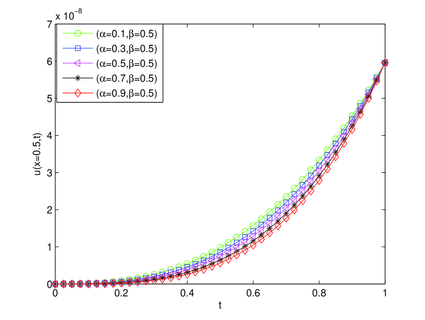
Figure 6.1: The numerical solution behaviours at $x=0.5$ by difference scheme (13) for different $\alpha$ and fixed $\beta=0.5$ with $\tau=\frac{1}{40}$ and $h=\frac{1}{100}$.

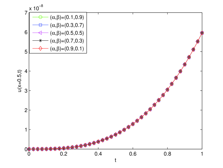
Figure 6.2: The numerical solution behaviours at $x=0.5$ by difference scheme (13) for different pairs $(\alpha,\beta)$ (which satisfy $\alpha+\beta=1$) with $\tau=\frac{1}{40}$ and $h=\frac{1}{100}$.

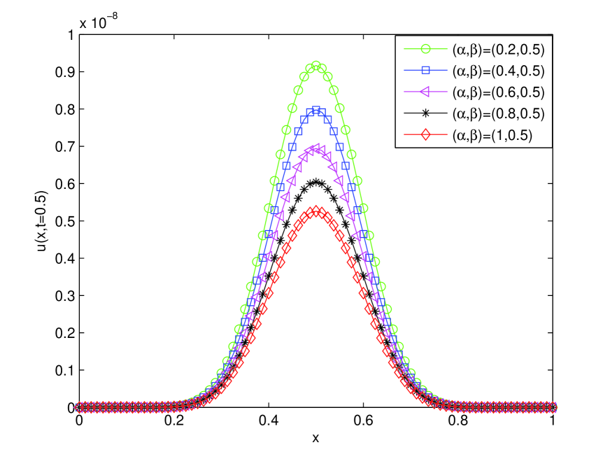
Figure 6.3: The numerical solution behaviours at $t=0.5$ by difference scheme (13) for different $\alpha$ and fixed $\beta=0.5$ with $\tau=\frac{1}{50}$ and $h=\frac{1}{80}$.

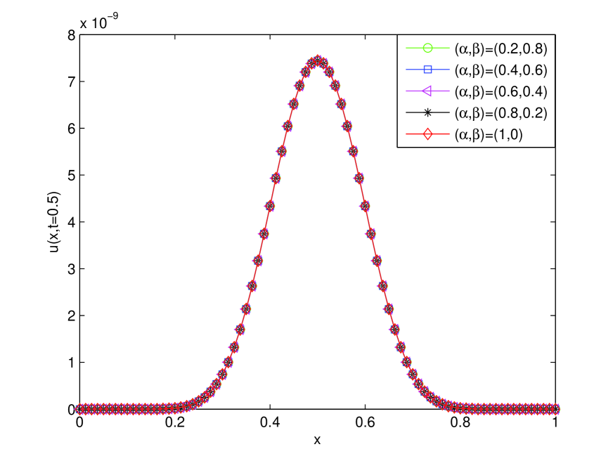
Figure 6.4: The numerical solution behaviours at $t=0.5$ by difference scheme (13) for different pairs $(\alpha,\beta)$ (which satisfy $\alpha+\beta=1$) with $\tau=\frac{1}{40}$ and $h=\frac{1}{100}$.

7 Conclusion

In this paper, we establish two high-order compact finite difference schemes for the modified anomalous subdiffusion equation. The stability and convergence conditions of the difference schemes are given by using the Fourier method. Finally, numerical experiments have been carried out to support the theoretical claims. These methods and techniques can be extended in a straightforward way to two or three spatial dimensional cases.

Appendix I:

The forms of the matrices $A,B,$ $\widetilde{A},\widetilde{B}$, $C_{k}$ and $\widetilde{C_{k}}$ are list as follows:

$$A=\left(\begin{array}[]{ccccccccc}\frac{14}{15}&\frac{2}{45}&-\frac{1}{90}&0&\cdots&0&0&0&0\vspace{0.2 cm}\\ \frac{2}{45}&\frac{14}{15}&\frac{2}{45}&-\frac{1}{90}&0&\cdots&0&0&0\vspace{0.2 cm}\\ -\frac{1}{90}&\frac{2}{45}&\frac{14}{15}&\frac{2}{45}&-\frac{1}{90}&0&\cdots&0&0\vspace{0.2 cm}\\ 0&-\frac{1}{90}&\frac{2}{45}&\frac{14}{15}&\frac{2}{45}&-\frac{1}{90}&0&\cdots&0\vspace{0.4 cm}\\ \vdots&\ddots&\ddots&\ddots&\ddots&\ddots&\ddots&\ddots&\vdots\vspace{0.4 cm}\\ 0&\cdots&0&-\frac{1}{90}&\frac{2}{45}&\frac{14}{15}&\frac{2}{45}&-\frac{1}{90}&0\vspace{0.2 cm}\\ 0&0&\cdots&0&-\frac{1}{90}&\frac{2}{45}&\frac{14}{15}&\frac{2}{45}&-\frac{1}{90}\vspace{0.2 cm}\\ 0&0&0&\cdots&0&-\frac{1}{90}&\frac{2}{45}&\frac{14}{15}&\frac{2}{45}\vspace{0.2 cm}\\ 0&0&0&0&\cdots&0&-\frac{1}{90}&\frac{2}{45}&\frac{14}{15}\vspace{0.2 cm}\\ \end{array}\right),$$

$$B=\left(\begin{array}[]{ccccccccc}-\frac{5}{2}&\frac{4}{3}&-\frac{1}{12}&0&\cdots&0&0&0&0\vspace{0.2 cm}\\ \frac{4}{3}&-\frac{5}{2}&\frac{4}{3}&-\frac{1}{12}&0&\cdots&0&0&0\vspace{0.2 cm}\\ -\frac{1}{12}&\frac{4}{3}&-\frac{5}{2}&\frac{4}{3}&-\frac{1}{12}&0&\cdots&0&0\vspace{0.2 cm}\\ 0&-\frac{1}{12}&\frac{4}{3}&-\frac{5}{2}&\frac{4}{3}&-\frac{1}{12}&0&\cdots&0\vspace{0.4 cm}\\ \vdots&\ddots&\ddots&\ddots&\ddots&\ddots&\ddots&\ddots&\vdots\vspace{0.4 cm}\\ 0&\cdots&0&-\frac{1}{12}&\frac{4}{3}&-\frac{5}{2}&\frac{4}{3}&-\frac{1}{12}&0\vspace{0.2 cm}\\ 0&0&\cdots&0&-\frac{1}{12}&\frac{4}{3}&-\frac{5}{2}&\frac{4}{3}&-\frac{1}{12}\vspace{0.2 cm}\\ 0&0&0&\cdots&0&-\frac{1}{12}&\frac{4}{3}&-\frac{5}{2}&\frac{4}{3}\vspace{0.2 cm}\\ 0&0&0&0&\cdots&0&-\frac{1}{12}&\frac{4}{3}&-\frac{5}{2}\vspace{0.2 cm}\\ \end{array}\right),$$

$$\widetilde{A}=\left(\begin{array}[]{ccccccccccc}\frac{27}{28}&\frac{3}{112}&-\frac{3}{280}&\frac{1}{560}&0&\cdots&0&0&0&0&0\vspace{0.2 cm}\\ \frac{3}{112}&\frac{27}{28}&\frac{3}{112}&-\frac{3}{280}&\frac{1}{560}&0&\cdots&0&0&0&0\vspace{0.2 cm}\\ -\frac{3}{280}&\frac{3}{112}&\frac{27}{28}&\frac{3}{112}&-\frac{3}{280}&\frac{1}{560}&0&\cdots&0&0&0\vspace{0.2 cm}\\ \frac{1}{560}&-\frac{3}{280}&\frac{3}{112}&\frac{27}{28}&\frac{3}{112}&-\frac{3}{280}&\frac{1}{560}&0&\cdots&0&0\vspace{0.2 cm}\\ 0&\frac{1}{560}&-\frac{3}{280}&\frac{3}{112}&\frac{27}{28}&\frac{3}{112}&-\frac{3}{280}&\frac{1}{560}&0&0&0\vspace{0.4 cm}\\ \vdots&\ddots&\ddots&\ddots&\ddots&\ddots&\ddots&\ddots&\ddots&\ddots&\vdots\vspace{0.4 cm}\\ 0&\cdots&0&\frac{1}{560}&-\frac{3}{280}&\frac{3}{112}&\frac{27}{28}&\frac{3}{112}&-\frac{3}{280}&\frac{1}{560}&0\vspace{0.2 cm}\\ 0&0&\cdots&0&\frac{1}{560}&-\frac{3}{280}&\frac{3}{112}&\frac{27}{28}&\frac{3}{112}&-\frac{3}{280}&\frac{1}{560}\vspace{0.2 cm}\\ 0&0&0&\cdots&0&\frac{1}{560}&-\frac{3}{280}&\frac{3}{112}&\frac{27}{28}&\frac{3}{112}&-\frac{3}{280}\vspace{0.2 cm}\\ 0&0&0&0&\cdots&0&\frac{1}{560}&-\frac{3}{280}&\frac{3}{112}&\frac{27}{28}&\frac{3}{112}\vspace{0.2 cm}\\ 0&0&0&0&0&\cdots&0&\frac{1}{560}&-\frac{3}{280}&\frac{3}{112}&\frac{27}{28}\vspace{0.2 cm}\\ \end{array}\right),$$

$$\widetilde{B}=\left(\begin{array}[]{ccccccccccc}-\frac{49}{18}&\frac{3}{2}&-\frac{3}{20}&\frac{1}{90}&0&\cdots&0&0&0&0&0\vspace{0.2 cm}\\ \frac{3}{2}&-\frac{49}{18}&\frac{3}{2}&-\frac{3}{20}&\frac{1}{90}&0&\cdots&0&0&0&0\vspace{0.2 cm}\\ -\frac{3}{20}&\frac{3}{2}&-\frac{49}{18}&\frac{3}{2}&-\frac{3}{20}&\frac{1}{90}&0&\cdots&0&0&0\vspace{0.2 cm}\\ \frac{1}{90}&-\frac{3}{20}&\frac{3}{2}&-\frac{49}{18}&\frac{3}{2}&-\frac{3}{20}&\frac{1}{90}&0&\cdots&0&0\vspace{0.2 cm}\\ 0&\frac{1}{90}&-\frac{3}{20}&\frac{3}{2}&-\frac{49}{18}&\frac{3}{2}&-\frac{3}{20}&\frac{1}{90}&0&\cdots&0\vspace{0.2 cm}\\ \vdots&\ddots&\ddots&\ddots&\ddots&\ddots&\ddots&\ddots&\ddots&\ddots&\vdots\vspace{0.4 cm}\\ 0&\cdots&0&\frac{1}{90}&-\frac{3}{20}&\frac{3}{2}&-\frac{49}{18}&\frac{3}{2}&-\frac{3}{20}&\frac{1}{90}&0\vspace{0.2 cm}\\ 0&0&\cdots&0&\frac{1}{90}&-\frac{3}{20}&\frac{3}{2}&-\frac{49}{18}&\frac{3}{2}&-\frac{3}{20}&\frac{1}{90}\vspace{0.2 cm}\\ 0&0&0&\cdots&0&\frac{1}{90}&-\frac{3}{20}&\frac{3}{2}&-\frac{49}{18}&\frac{3}{2}&-\frac{3}{20}\vspace{0.2 cm}\\ 0&0&0&0&\cdots&0&\frac{1}{90}&-\frac{3}{20}&\frac{3}{2}&-\frac{49}{18}&\frac{3}{2}\vspace{0.2 cm}\\ 0&0&0&0&0&\cdots&0&\frac{1}{90}&-\frac{3}{20}&\frac{3}{2}&-\frac{49}{18}\vspace{0.2 cm}\\ \end{array}\right),$$

$$\begin{array}[]{l}\displaystyle C_{k}=\left(\begin{array}[]{c}\left(\frac{1}{90}-\frac{1}{12}g_{0}^{(\alpha,\beta)}\right)u_{-1}^{k+1}-\left(\frac{1}{90}+\frac{1}{12}g_{1}^{(\alpha,\beta)}\right)u_{-1}^{k}-\frac{1}{12}\sum\limits_{\ell=2}^{k+1}g_{\ell}^{(\alpha,\beta)}u_{-1}^{k+1-\ell}\vspace{0.2 cm}\\ -\left(\frac{2}{45}-\frac{4}{3}g_{0}^{(\alpha,\beta)}\right)u_{0}^{k+1}+\left(\frac{2}{45}+\frac{4}{3}g_{1}^{(\alpha,\beta)}\right)u_{0}^{k}+\frac{4}{3}\sum\limits_{\ell=2}^{k+1}g_{\ell}^{(\alpha,\beta)}u_{0}^{k+1-\ell}\vspace{0.2 cm}\\ -\frac{1}{90}\tau f_{-1}^{k+\frac{1}{2}}+\frac{2}{45}\tau f_{0}^{k+\frac{1}{2}},\vspace{0.4 cm}\\ \left(\frac{1}{90}-\frac{1}{12}g_{0}^{(\alpha,\beta)}\right)u_{0}^{k+1}-\left(\frac{1}{90}+\frac{1}{12}g_{1}^{(\alpha,\beta)}\right)u_{0}^{k}-\frac{1}{12}\sum\limits_{\ell=2}^{k+1}g_{\ell}^{(\alpha,\beta)}u_{0}^{k+1-\ell}-\frac{1}{90}\tau f_{0}^{k+\frac{1}{2}},\vspace{0.4 cm}\\ 0\vspace{0.4 cm}\\ \vdots\vspace{0.4 cm}\\ 0\vspace{0.4 cm}\\ \left(\frac{1}{90}-\frac{1}{12}g_{0}^{(\alpha,\beta)}\right)u_{M}^{k+1}-\left(\frac{1}{90}+\frac{1}{12}g_{1}^{(\alpha,\beta)}\right)u_{M}^{k}-\frac{1}{12}\sum\limits_{\ell=2}^{k+1}g_{\ell}^{(\alpha,\beta)}u_{M}^{k+1-\ell}-\frac{1}{90}\tau f_{M}^{k+\frac{1}{2}},\vspace{0.4 cm}\\ \left(\frac{1}{90}-\frac{1}{12}g_{0}^{(\alpha,\beta)}\right)u_{M+1}^{k+1}-\left(\frac{1}{90}+\frac{1}{12}g_{1}^{(\alpha,\beta)}\right)u_{M+1}^{k}-\frac{1}{12}\sum\limits_{\ell=2}^{k+1}g_{\ell}^{(\alpha,\beta)}u_{M+1}^{k+1-\ell}\vspace{0.2 cm}\\ -\left(\frac{2}{45}-\frac{4}{3}g_{0}^{(\alpha,\beta)}\right)u_{M}^{k+1}+\left(\frac{2}{45}+\frac{4}{3}g_{1}^{(\alpha,\beta)}\right)u_{M}^{k}+\frac{4}{3}\sum\limits_{\ell=2}^{k+1}g_{\ell}^{(\alpha,\beta)}u_{M}^{k+1-\ell}\vspace{0.2 cm}\\ -\frac{1}{90}\tau f_{M+1}^{k+\frac{1}{2}}+\frac{2}{45}\tau f_{M}^{k+\frac{1}{2}}\end{array}\right),\end{array}$$

$$\begin{array}[]{l}\displaystyle\widetilde{C}_{k}=\left(\begin{array}[]{c}-\left(\frac{1}{560}-\frac{1}{90}g_{0}^{(\alpha,\beta)}\right)u_{-2}^{k+1}+\left(\frac{1}{560}+\frac{1}{90}g_{1}^{(\alpha,\beta)}\right)u_{-2}^{k}+\frac{1}{90}\sum\limits_{\ell=2}^{k+1}g_{\ell}^{(\alpha,\beta)}u_{-2}^{k+1-\ell}\\ +\left(\frac{3}{280}-\frac{3}{20}g_{0}^{(\alpha,\beta)}\right)u_{-1}^{k+1}-\left(\frac{3}{280}+\frac{3}{20}g_{1}^{(\alpha,\beta)}\right)u_{-1}^{k}-\frac{3}{20}\sum\limits_{\ell=2}^{k+1}g_{\ell}^{(\alpha,\beta)}u_{-1}^{k+1-\ell}\\ -\left(\frac{1}{112}-\frac{3}{2}g_{0}^{(\alpha,\beta)}\right)u_{0}^{k+1}+\left(\frac{1}{112}+\frac{3}{2}g_{1}^{(\alpha,\beta)}\right)u_{0}^{k}+\frac{3}{2}\sum\limits_{\ell=2}^{k+1}g_{\ell}^{(\alpha,\beta)}u_{0}^{k+1-\ell}\\ +\frac{1}{560}\tau f_{-2}^{k+\frac{1}{2}}-\frac{3}{280}\tau f_{-1}^{k+\frac{1}{2}}+\frac{1}{112}\tau f_{0}^{k+\frac{1}{2}},\vspace{0.1 cm}\\ -\left(\frac{1}{560}-\frac{1}{90}g_{0}^{(\alpha,\beta)}\right)u_{-1}^{k+1}+\left(\frac{1}{560}+\frac{1}{90}g_{1}^{(\alpha,\beta)}\right)u_{-1}^{k}+\frac{1}{90}\sum\limits_{\ell=2}^{k+1}g_{\ell}^{(\alpha,\beta)}u_{-1}^{k+1-\ell}\\ +\left(\frac{3}{280}-\frac{3}{20}g_{0}^{(\alpha,\beta)}\right)u_{0}^{k+1}-\left(\frac{3}{280}+\frac{3}{20}g_{1}^{(\alpha,\beta)}\right)u_{0}^{k}-\frac{3}{20}\sum\limits_{\ell=2}^{k+1}g_{\ell}^{(\alpha,\beta)}u_{0}^{k+1-\ell}\\ +\frac{1}{560}\tau f_{-1}^{k+\frac{1}{2}}-\frac{3}{280}\tau f_{0}^{k+\frac{1}{2}},\vspace{0.1 cm}\\ -\left(\frac{1}{560}-\frac{1}{90}g_{0}^{(\alpha,\beta)}\right)u_{0}^{k+1}+\left(\frac{1}{560}+\frac{1}{90}g_{1}^{(\alpha,\beta)}\right)u_{0}^{k}+\frac{1}{90}\sum\limits_{\ell=2}^{k+1}g_{\ell}^{(\alpha,\beta)}u_{0}^{k+1-\ell}+\frac{1}{560}\tau f_{0}^{k+\frac{1}{2}},\vspace{0.2 cm}\\ 0\vspace{0.2 cm}\\ \vdots\vspace{0.2 cm}\\ 0\vspace{0.1 cm}\\ -\left(\frac{1}{560}-\frac{1}{90}g_{0}^{(\alpha,\beta)}\right)u_{M}^{k+1}+\left(\frac{1}{560}+\frac{1}{90}g_{1}^{(\alpha,\beta)}\right)u_{M}^{k}+\frac{1}{90}\sum\limits_{\ell=2}^{k+1}g_{\ell}^{(\alpha,\beta)}u_{M}^{k+1-\ell}+\frac{1}{560}\tau f_{M}^{k+\frac{1}{2}},\vspace{0.1 cm}\\ -\left(\frac{1}{560}-\frac{1}{90}g_{0}^{(\alpha,\beta)}\right)u_{M+1}^{k+1}+\left(\frac{1}{560}+\frac{1}{90}g_{1}^{(\alpha,\beta)}\right)u_{M+1}^{k}+\frac{1}{90}\sum\limits_{\ell=2}^{k+1}g_{\ell}^{(\alpha,\beta)}u_{M+1}^{k+1-\ell}\\ +\left(\frac{3}{280}-\frac{3}{20}g_{0}^{(\alpha,\beta)}\right)u_{M}^{k+1}-\left(\frac{3}{280}+\frac{3}{20}g_{1}^{(\alpha,\beta)}\right)u_{M}^{k}-\frac{3}{20}\sum\limits_{\ell=2}^{k+1}g_{\ell}^{(\alpha,\beta)}u_{M}^{k+1-\ell}\\ +\frac{1}{560}\tau f_{M+1}^{k+\frac{1}{2}}-\frac{3}{280}\tau f_{M}^{k+\frac{1}{2}},\vspace{0.1 cm}\\ -\left(\frac{1}{560}-\frac{1}{90}g_{0}^{(\alpha,\beta)}\right)u_{M+2}^{k+1}+\left(\frac{1}{560}+\frac{1}{90}g_{1}^{(\alpha,\beta)}\right)u_{M+2}^{k}+\frac{1}{90}\sum\limits_{\ell=2}^{k+1}g_{\ell}^{(\alpha,\beta)}u_{M+2}^{k+1-\ell}\\ +\left(\frac{3}{280}-\frac{3}{20}g_{0}^{(\alpha,\beta)}\right)u_{M+1}^{k+1}-\left(\frac{3}{280}+\frac{3}{20}g_{1}^{(\alpha,\beta)}\right)u_{M+1}^{k}-\frac{3}{20}\sum\limits_{\ell=2}^{k+1}g_{\ell}^{(\alpha,\beta)}u_{M+1}^{k+1-\ell}\\ -\left(\frac{1}{112}-\frac{3}{2}g_{0}^{(\alpha,\beta)}\right)u_{M}^{k+1}+\left(\frac{1}{112}+\frac{3}{2}g_{1}^{(\alpha,\beta)}\right)u_{M}^{k}+\frac{3}{2}\sum\limits_{\ell=2}^{k+1}g_{\ell}^{(\alpha,\beta)}u_{M}^{k+1-\ell}\\ +\frac{1}{560}\tau f_{M+2}^{k+\frac{1}{2}}-\frac{3}{280}\tau f_{M+1}^{k+\frac{1}{2}}+\frac{1}{112}\tau f_{M}^{k+\frac{1}{2}}\end{array}\right).\end{array}$$

Appendix II:

(i) In the finite difference scheme (13), we use the following sixth-order extrapolation formulas for the ghost-point values:

$$\begin{array}[]{lll}\displaystyle u_{-1}^{k}=6u_{0}^{k}-15u_{1}^{k}+20u_{2}^{k}-15u_{3}^{k}+6u_{4}^{k}-u_{5}^{k}+\mathcal{O}(h^{6}),\end{array}$$

and

$$\begin{array}[]{lll}\displaystyle u_{M+1}^{k}=6u_{M}^{k}-15u_{M-1}^{k}+20u_{M-2}^{k}-15u_{M-3}^{k}+6u_{M-4}^{k}-u_{M-5}^{k}+\mathcal{O}(h^{6}).\end{array}$$

(ii) In the finite difference scheme (14), we use the following eighth-order extrapolation formulas for the ghost-point values:

$$\begin{array}[]{lll}\displaystyle u_{-1}^{k}=8u_{0}^{k}-28u_{1}^{k}+56u_{2}^{k}-70u_{3}^{k}+56u_{4}^{k}-28u_{5}^{k}+8u_{6}^{k}-u_{7}^{k}+\mathcal{O}(h^{8}),\end{array}$$

$$\begin{array}[]{lll}\displaystyle u_{-2}^{k}=36u_{0}^{k}-168u_{1}^{k}+378u_{2}^{k}-504u_{3}^{k}+420u_{4}^{k}-216u_{5}^{k}+63u_{6}^{k}-8u_{7}^{k}+\mathcal{O}(h^{8}),\end{array}$$

$$\begin{array}[]{lll}\displaystyle u_{M+1}^{k}=8u_{M}^{k}-28u_{M-1}^{k}+56u_{M-2}^{k}-70u_{M-3}^{k}+56u_{M-4}^{k}-28u_{M-5}^{k}+8u_{M-6}^{k}-u_{M-7}^{k}+\mathcal{O}(h^{8}),\end{array}$$

and

$$\begin{array}[]{lll}\displaystyle u_{M+2}^{k}=&\displaystyle 36u_{M}^{k}-168u_{M-1}^{k}+378u_{M-2}^{k}-504u_{M-3}^{k}+420u_{M-4}^{k}-216u_{M-5}^{k}+63u_{M-6}^{k}\vspace{0.2 cm}\\ &\displaystyle-8u_{M-7}^{k}+\mathcal{O}(h^{8}).\end{array}$$

References

- [1] A. Compte, R. Metzler, The generalized cattaneo equation for the description of anomalous transport processes, J. Phys. A: Math. Gen., 30 (1997) 7277–7289.
- [2] J. Crank, The mathematics of diffusion, Oxford University Press, Clarendon, 1975.
- [3] I. M. Sokolov, A. V. Chechkin, J. Klafter, Fractional diffusion equation for a power-law-truncated Lévy process, Physica A, 336 (2004) 245–251.
- [4] I. Sokolov, J. Klafter, From diffusion to anomalous diffusion: A century after Einstein’s Brownian motion, Chaos, 15 (2005) 026103.
- [5] A. V. Chechkin, R. Gorenflo, I. M. Sokolov, V. Y. Gonchar, Distributed order time fractional diffusion equation, Fract. Calc. Appl. Anal., 6 (2003) 259–279.
- [6] T. A. M. Langlands, Solution of a modified fractional diffusion equation, Physica A., 367 (2006) 136–144.
- [7] H. Wang, K. X. Wang, T. Sircar, A direct finite difference method for fractional diffusion equations, J. Comput. Phys., 229 (2010) 8095–8104.
- [8] C. M. Chen, F. Liu, I. Turner, V. Anh, A Fourier method for the fractional diffusion equation describing sub-diffusion, J. Comput. Phys., 227 (2007) 886–897.
- [9] F. H. Zeng, C. P. Li, F. W. Liu, I. Turner, The use of finite difference/element approaches for solving the time-fractional subdiffusion equation, SIAM J. Sci. Comput. 35 (2013) A2976–A3000.
- [10] F. H. Zeng, C. P. Li, F. W. Liu, I. Turner, Numerical algorithms for time-fractional subdiffusion equation with second-order accuracy, SIAM J. Sci. Comput. 37 (2015) A55–A78.
- [11] S. B. Yuste, L. Acedo, An explicit finite difference method and a new von Neumann-tape stability analysis for fractional diffusion equations, SIAM J. Numer. Anal., 42 (2005) 1862–1874.
- [12] H. Zhou, W. Tian, W. Deng, Quasi-compact finite difference schemes for space fractional diffusion equations, J. Sci. Comput., 56 (2013) 45–66.
- [13] M. Meerschaert, C. Tadjeran, Finite difference approximations for fractional advectiondispersion flow equations, J. Comput. Appl. Math., 172 (2004) 65–77.
- [14] J. Huang, Y. Tang, L. Vazquez, J. Yang, Two finite difference schemes for time fractional diffusion-wave equation, Numer. Algor., 64 (2013) 707–720.
- [15] S. Chen, X. Jiang, F. Liu, I. Turner, High order unconditionally stable difference schemes for the Riesz space-fractional telegraph equation, J. Comput. Appl. Math., 278 (2015) 119–129.
- [16] H. Wang, X. Zhang, A high-accuracy preserving spectral Galerkin method for the Dirichlet boundary-value problem of variable-coefficient conservative fractional diffusion equations, J. Comput. Phys., 281 (2015) 67–81.
- [17] A. A. Alikhanov, A new difference scheme for the time fractional diffusion equation, J. Comput. Phys., 280 (2015) 424–438.
- [18] W. Jiang, Z. Chen, A collocation method based on reproducing kernel for a modified anomalous subdiffusion equation, Numer. Meth. Part. D. E., 27 (2011) 1599–1609.
- [19] F. Liu, C. Yang, K. Burrage, Numerical method and analytical technique of the modified anomalous subdiffusion equation with a nonlinear source term, J. Comput. Appl. Math., 231 (2009) 160–176.
- [20] A. Mohebbi, M. Abbaszade, M. Dehghan, A high-order and unconditionally stable scheme for the modified anomalous fractional sub-diffusion equation with a nonlinear source term, J. Comput. Phys., 240 (2013) 36–48.
- [21] Z. Wang, S. Vong, Compact difference schemes for the modified anomalous fractional sub-diffusion equation and the fractional diffusion-wave equation, arXiv:1310.5298v2.
- [22] M. R. Cui, Compact finite difference method for the fractional diffusion equation, J. Comput. Phys., 228 (2009) 7792–7804.
- [23] W. F. Ames, Numerical Methods for Partial Differential Equations, Academic Press, New York, 1977.
- [24] A. Quarteroni, R. Sacco, F. Saleri, Numerical Mathematics, Springer, New York, 2007.
- [25] V. K. Tuan, R. Gorenflo, Extrapolation to the Limit for Numerical Fractional Differentiation, Z. angew. Math. Mech., 75 (1995) 646–648.
- [26] U. Grenander, G. Szegö, Toeplitz Forms and Their Applications, University of Calif. Press, Berkeley and Los Angeles, 1958.
- [27] C. P. Li, H. F. Ding, Higher order finite difference method for the reaction and anomalous-diffusion equation, Appl. Math. Model., 38 (2014) 3802–3821.
- [28] J. Masoliver, M. Montero, J. Perello, G.H. Weiss, The continuous time random walk formalism in financial markets, J. Econ. Behav. Org., 61 (2006) 577–591.
- [29] R. Metzler, J. Klafter, The random walk s guide to anomalous diffusion: a fractional dynamics approach, Phys. Rep., 339 (2000) 1–77.