Time-irreversibility of the statistics of a single particle in a compressible turbulence

Abstract

We investigate time-irreversibility from the point of view of a single particle in Burgers turbulence. Inspired by the recent work for incompressible flows [Xu et al., PNAS 111.21 (2014) 7558], we analyze the evolution of the kinetic energy for fluid markers and use the fluctuations of the instantaneous power as a measure of time-irreversibility. For short times, starting from a uniform distribution of markers, we find the scaling $\left<[E(t)-E(0)]^{n}\right>\propto t$ and $\left<p^{n}\right>\propto\mathrm{Re}^{n-1}$ for the power as a function of the Reynolds number. Both observations can be explained using the “flight-crash” model, suggested by Xu et al. Furthermore, we use a simple model for shocks which reproduces the moments of the energy difference including the pre-factor for $\left<E(t)-E(0)\right>$. To complete the single particle picture for Burgers we compute the moments of the Lagrangian velocity difference and show that they are bi-fractal. This arises in a similar manner to the bi-fractality of Eulerian velocity differences. In the above setting, time-irreversibility is directly manifest as particles eventually end up in shocks. We additionally investigate time-irreversibility in the long-time limit when all particles are located inside shocks and the Lagrangian velocity statistics are stationary. We find the same scalings for the power and energy differences as at short times and argue that this is also a consequence of rare “flight-crash” events related to shock collisions.

I Introduction

One may think that since viscous friction is responsible for flow irreversibility, the latter must disappear in the inviscid limit. On the contrary, there exists a dimensionless measure of irreversibility that actually grows unbounded as the viscosity goes to zero, as was recently found for incompressible turbulence xu-pumir-etal:2014 and as we show here for a compressible one. The reason is that when the magnitude and scale of the flow excitation is fixed while the viscosity is getting smaller the fluid is driven away from equilibrium. This is a consequence of the persistence of energy dissipation at smaller and smaller scales as viscosity tends to zero (i.e $\mathrm{Re}\to\infty$). At equilibrium, time reversibility of the statistics is manifest through detailed balance: It is equally probable for energy to transfer between two scales of the flow in either direction onsager:1931 . On the contrary, in a steady state of a turbulent flow, the separation between the scale at which energy is introduced and that at which it is dissipated is of the order of the Reynolds number and an energy flux is formed between the two frisch:1995 .

In other words, at equilibrium detailed balance means that excitation and dissipation are balanced at every scale and every timescale. In turbulence, by increasing the ratio of excitation and dissipation scales we naturally drive the system further from equilibrium. In light of this discussion it is clear that a measure of time-irreversibility should be at the same time a measure of the deviation from equilibrium. The question now is how to recover such a measure not by looking at the spatial structure of forcing and dissipation in the whole system (as done e.g. in bauer-bernard:1999 ; eyink-drivas:2014 ), but by studying the temporal evolution of the smallest part of the flow, a single fluid element. It requires some work to devise a measure of time-irreversibility that can be measured using single particle statistics: the velocity statistics are stationary implying that velocity structure functions are invariant under $t\rightarrow-t$ falkovich-etal:2012 . Xu et al. xu-pumir-etal:2014 suggested to study the statistics of the energy evolution of a fluid particle, $W(t)=\frac{1}{2}(u(t)^{2}-u(0)^{2})$, and showed that here irreversibility is embodied as follows: a particle gains energy slowly and loses it fast, a process they termed “flight-crash” events. A measure of time-irreversibility, Ir, was then constructed by looking at the short time limit of $W(t)$, the power $p=\bf{a}\cdot\bf{v}$ where $a$ is the Lagrangian acceleration, and it was found that $\textit{Ir}\equiv-\left<p^{3}\right>/\epsilon^{3}\propto\mathrm{Re}^{2}$, where $\epsilon$ is the dissipation rate of kinetic energy. This scaling and the skewness of the statistics of single particle energy changes was hypothesized to originate from the “flight-crash” events.

In this paper, we want to apply similar techniques to measure time-irreversibility in a compressible flow in two setups. “Flight-crash” events are expected to be present in compressible turbulence from a general point of view: for strongly compressible high-$\mathrm{Re}$ flows particles travel mostly unaffected until colliding with other particles inside shocks beetz-etal:2008 , a process during which they rapidly lose energy. The Burgers equation driven by a large-scale force describes a set of distant shocks bec-khanin:2007 and is therefore a good test bed for ideas about “flight-crash” events as a source of irreversibility. It can also serve as a simple model to explore irreversibility in strongly compressible turbulent flows.

First we sample markers initially homogeneously distributed in the flow. For the energy increments we find similarly skewed statistics to those found in xu-pumir-etal:2014 , $\langle W^{3}\rangle<0$ and the scaling $\langle W^{n}\rangle\propto t$ which can be explained by dominance of “flight-crash” events as well as, in more detail, by modeling the fall of particles into shocks. We furthermore analyze the power $p$ of particles and its moments, which also depend on $\mathrm{Re}$ in this case. Its scaling with $\mathrm{Re}$ agrees with estimates of the relation between the shock width and viscosity as well as the prediction from a “flight-crash” model. Note that this type of sampling results in non-stationary Lagrangian velocity statistics due to compressibility, making time-irreversibility more evident. In particular the connection between $W(t)$ and $W(-t)$ is not simply a sign flip.

In the second setting, we examine the long time limit, in which all particles are located inside shocks. In this limit the velocity statistics are stationary and time-irreversibility is less transparent. We show that again moments of $W(t)$ and of the power can be used to measure irreversibility and display the same qualitative features as their short time counterparts. These results can also be interpreted to arise from a “flight-crash” model where the crashes leading to a sudden energy change are shock collisions.

The paper is organized as follows: In Sec. II we introduce a setting and establish a qualitative model of particle trajectories in a turbulent flow, the so called “flight-crash”-model. We show that this model has a direct interpretation in compressible turbulence, as particles crashing into shocks rapidly lose energy. To estimate particle energy increments we invoke a steady state shock model in Sec. III. The predictions from this model are then compared to numerical simulations of 1d compressible turbulence, both for energy increments, in Sec. III and IV, and moments of power in Sec. V. We then investigate Lagrangian velocity increments, in Sec. VI, comparing results from numerical simulations to predictions based on the competition between forcing induced propagation and events related to shocks. In the last part, Sec. VII, we try to eliminate the effect of compressibility which induces non stationary statistics of velocities by looking at the long time statistics for a single particle. Our main result is a numerical verification of these estimates in both setups.

II “Flight-Crash” events in compressible turbulence

In the following we consider the Burgers equation burgers:1974 ,

$$v_{t}+vv_{x}-\nu v_{xx}=f\,,$$ (1)

as a simple model for a compressible flow in 1d, where $f$ is the forcing term. Particles at position $x(t)$ are advected with the velocity $v(x(t),t)$, obeying the equation

$$\frac{\mathrm{d}x(t)}{\mathrm{d}t}=v(x(t),t),\qquad x(0)=x_{0}\,.$$ (2)

We furthermore denote the particle velocity with $v(x(t),t)=u(t)$. The quantities that are of interest to us are the moments of kinetic energy differences along trajectories of fluid elements, $\langle W(t)^{n}\rangle$, as well as moments of the instantaneous power for fluid elements distributed homogeneously, $\left<(a(0)v(0))^{n}\right>$.

All numerical simulations carried out for this work integrate equation (1) in time, using a second order stochastic Runge-Kutta algorithm honeycutt:1992 in time and fast Fourier transforms for all space derivatives. The tracer particles are integrated with the same time-marching algorithm and a second-order field interpolation. For stochastic forcing we employ both Brownian noise with $\delta(t)$ correlation in time and finitely correlated noise with correlation time $T_{f}$ implemented as an Ornstein-Uhlenbeck process in Fourier space eswaran-pope:1988 , depending on the physical requirements. The Reynolds number is varied in the range $10^{1}<\mathrm{Re}<10^{4}$. Different $\mathrm{Re}$ are achieved by modifying $\nu$ while retaining the shape of the forcing. The implementation uses graphics processing units (GPU) and the CUDA framework cuda:2014 for speedup and allows us to reach $10^{8}$–$10^{10}$ computational steps, which amounts to approximately $10^{4}$–$10^{5}$ integral times per simulation.

In Burgers turbulence bec-khanin:2007 , a finite number of shock structures, i.e. subsets with a large $\partial_{x}v$, emerge with a density $\rho=1/L$, where $L$ is the forcing correlation length. These structures capture surrounding particles. Regions between shocks are comparably smooth, and the relative motion between particles in those regions and the neighboring shocks is approximately ballistic. If particles are injected with a uniform distribution at $t=0$, almost all of them are initially located in the smooth regions between the shocks. Each particle then undergoes a ballistic motion with respect to the nearest shock until crashing into it. In terms of the energy difference at time $t$, there are therefore two types of events that one expects to contribute: The most common events are those where the particle gains energy slowly due to the forcing far away from any shock; the rare events occur when the particle enters a shock during the time $t$, losing a large amount of energy. The latter events are naturally interpreted as “flight-crash”-events and give the largest contribution to the energy difference.

Following the derivation of this model in the incompressible case, let us evaluate the contribution of the rare events in which energy is lost giving $W<0$. First we use the decomposition $\langle W(t)^{n}\rangle\approx\langle\left(v_{\text{rms}}(u(t)-u(0))\right)^{n}\rangle$ and apply the estimate $(u(t)-u(0))\approx(v(r)-v(0))$ with $r=v_{\text{rms}}t$ the initial distance between the particle and the shock it enters for sufficiently short times. Then the Eulerian scaling $\langle(v(r)-v(0))^{n}\rangle\propto r$ implies the scaling $\langle W^{n}\rangle\propto t$ for $n>1$. As the Eulerian moments are not self similar the energy difference is not self similar either. Note that although we also get that $\langle W^{3}\rangle\propto t$, as in the prediction in the incompressible case, this is not a general feature of a “flight-crash”-type of argument but rather depends on the scaling of the third order Eulerian structure function.

Our estimate for $W$ also allows us to obtain predictions for the scaling of the power with the $\mathrm{Re}$. The scaling we derived above is expected to hold for times $t\geq\tau_{\eta}$, $\tau_{\eta}$ being the viscous time scale after which the internal structure of the shock does not matter. At times $t\leq\tau_{\eta}$ a Taylor expansion in time implies $\left<W^{n}\right>\propto\left<p^{n}\right>t^{n}$. At $t=\tau_{\eta}$ these two scalings should match, giving $\left<p^{n}\right>\propto\tau_{\eta}^{1-n}\propto\mathrm{Re}^{n-1}$. Note in passing that there is also an upper bound for our prediction for $W(t)$, $t<T_{L}$, with $T_{L}$ the typical time related to the forcing scale $L$. Up to this time the spatial variation of the forcing is not yet felt by the particle. For forcing with a finite time correlation there is an additional time scale, which we take to be of the order of $T_{L}$.

To summarize, according to the “flight-crash” model we expect to find $\left<p^{n}\right>\propto\mathrm{Re}^{n-1}$ for the power moments and $\left<W^{n}\right>\propto t$ for the energy difference. We will substantiate these estimates in the following sections.

III Moments of energy differences along fluid trajectories

Figure 1: Prototypical shock solution of the Burgers equation. The shock height is $2w$ and the shock velocity is $\bar{u}$. Particles on the brink of the shock enter the shock and lose energy. The amount of particles that enter the shock in time $t$ from the left or right side is $wt$.

Let us study the energy differences in more detail. From $u^{2}=u_{0}^{2}+2\int uf\,dt+2\nu\int uu_{xx}\,dt$ we can write $W(t)=\int uf\,dt+\nu\int uu_{xx}\,dt=F(t)+D(t)$ with $D(t)=\nu\int uu_{xx}\,dt$ being the amount of energy dissipated at the particle position and $F(t)$ the contribution to the energy from the forcing. The forcing term can be estimated as follows: initially, due to the balance between forcing and dissipation $\left<uf\right>=\epsilon$, meaning that its average is $\left<F\right>=\int\left<uf\right>\,dt=\epsilon t+O(t^{2})$ and for the higher moments we can use $\left<F^{n}\right>=O(t^{n})$. To evaluate the dissipation term we cannot use the latter argument, relying on a Taylor expansion, for times $t>\tau_{\eta}$ frishman-falkovich:2014 . Instead, anticipating that the main contribution to $D$ comes from shocks, we will use the simplest model of a shock to get estimates on $D$. Within this model we will compute the energy loss along particle trajectories for a given shock and then average over the shock parameters frishman-falkovich:2014 .

Consider a prototypical shock solution of the Burgers equation, as depicted in figure 1. Let the shock height be $2w$ and the shock velocity be $\bar{u}$. Then, particles entering from left and right lose different amounts of energy:

$$D_{1} =-\frac{1}{2}w^{2}-w\bar{u}$$

$$D_{2} =-\frac{1}{2}w^{2}+w\bar{u}.$$

The probability of a particle to enter a shock during time t, from either side of it, is $wt\rho$ where the shock density is related to the forcing scale $\rho=1/L$. Thus $\langle D\rangle=-\langle w^{2}\frac{wt}{L}\rangle=\frac{3}{2}\epsilon t$ falkovich2011fluid . Finally, adding the contribution from the forcing one obtains

$$\left<W\right>=-\frac{1}{2}\epsilon t.$$ (3)

for $\tau_{\eta}<t<T_{L}$. This estimated scaling in $\epsilon$ and $t$, as well as the pre-factor, agree well with numerical simulations using a white in time correlated forcing, as shown in figure 2. Corroborating this result for a finite correlated forcing requires a significant increase of the statistics as well as of the correlation time $T_{f}\approx T_{L}$ compared to those we used. While we did not attempt to do so, the partial results we obtained did not seem to contradict (3). Equation (3) demonstrates the main difference between Burgers and incompressible turbulence — the Lagrangian energy is not stationary; for short times, fluid elements lose energy linearly in time, on average, as opposed to $\langle W(t)\rangle=0$ in the incompressible case.

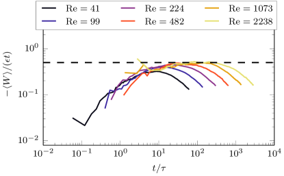
Figure 2: (Color online) $-\langle W(t)\rangle$ versus $t/\tau$, compensated by $\epsilon$ and $t$, for stationary Burgers turbulence, considering particles that start at a random position at $t=0$. Particles on average lose energy linearly in time, in accordance to the analytical estimate in equation (3).

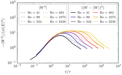
Figure 3: (Color online) In the inertial range, the centered moment (solid) $\langle(W-\langle W\rangle)^{3}\rangle$ scales similar to to $\langle W^{3}\rangle$ (dotted), which is in accordance with the analytical estimate in equation (4).

Turning to $\langle W^{3}\rangle$, it is dominated by $\langle D^{3}\rangle$ in the inertial range since the terms involving the forcing are sub-dominant by at least one factor of $t/T_{L}$. Thus one obtains

$$\left<W^{3}\right>\approx\left<D^{3}\right>=\left<\frac{wt}{L}\left(D_{1}^{3}+D_{2}^{3}\right)\right>=-\frac{t}{4L}\left<12\bar{u}^{2}w^{5}+w^{7}\right>.$$

For white in time forcing this equation can be re-expressed in terms of Eulerian velocity moments using

$$\left<v^{4}\right>=\frac{70\left<\bar{u}^{4}w^{3}\right>+84\left<\bar{u}^{2}w^{5}\right>+6\left<w^{7}\right>}{105L\epsilon}$$

from e-vandeneijnden:2000 to substitute for $\left<w^{7}\right>$ and thus obtain the bound

$$-\left<W^{3}\right><\frac{35}{2}\epsilon t\frac{\left<v^{4}\right>}{4}\,.$$ (4)

We present $\left<W^{3}\right>$ for white in time correlated forcing in figure 3 (dotted). The expected scaling with $t$ and $\epsilon$ is supported by the numerical results, the plateau increasing in length for growing Reynolds numbers. Furthermore it is evident that the bound in Eq. (4) is satisfied. We reproduce the same qualitative behavior with finite-time correlated forcing. This result is much easier to obtain than the one for $\left<W\right>$ as the forcing enters only sub-dominant terms in $\left<W^{3}\right>$ in the inertial interval.

Similarly, for a general moment $\langle W^{n}\rangle$ we expect

$$\left<W^{n}\right>\approx t$$

regardless of $n$, the dissipative term giving the dominating contribution for all $n>1$, $\langle W^{n}\rangle\approx\langle D^{n}\rangle$.

IV Centered moments of energy differences

For a compressible flow there is an obvious source of irreversibility for an initially homogeneous distribution of particles in space, since the particle density changes in time. This is why, unlike for the incompressible flow, already the first moment of $W$ shows irreversibility: $\langle W\rangle<0$. One might wonder whether by subtracting this average, i.e looking at centered moments $\langle(W-\langle W\rangle)^{n}\rangle$, it is possible to eliminate the footprints of irreversibility. In other words, subtracting the mean brings the situation closer to the incompressible case, with a random variable whose mean vanishes and its third centered moment being non-zero demonstrates irreversibility. This is indeed the case but the irreversibility in time is still dominated by the (linearly in time) increasing probability for a particle to crash into a shock.

In fact, we expect that the leading contribution would come from $\langle W^{3}\rangle\propto t$ rather than from $\langle W\rangle^{3}\approx O((t/T_{L})^{2})\langle W^{3}\rangle$ and $\langle W^{2}\rangle\langle W\rangle\approx O((t/T_{L}))\langle W^{3}\rangle$.

We can also use the above model to estimate the difference between $\langle(W-\langle W\rangle)^{3}\rangle$ and $\langle W^{3}\rangle$:

$$\left<(W-\left<W\right>)^{3}\right>=\left<W^{3}\right>-3\left<W^{2}\right>\left<W\right>+2\left<W\right>^{3}$$ (5)

Then, subtracting this from $\langle W^{3}\rangle$ to leading order in $t/T_{L}$ we have

$$-\left<W^{3}\right>+\left<(W-\left<W\right>)^{3}\right>\approx\frac{3}{2}\left<D^{2}\right>\epsilon t$$ (6)

after using $-3\left<W^{2}\right>\left<W\right>\approx-3\left<D^{2}\right>\left<W\right>=3/2\left<D^{2}\right>\epsilon t$. We therefore expect for times $t\approx T_{L}$, when this sub-leading term becomes visible, that the negative of the centered moment would lie lower than $-\left<W^{3}\right>$ . As shown in figure 3 (solid lines), this is consistent with what is observed in the numerical simulation.

V Moments of power

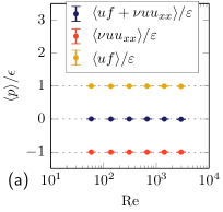
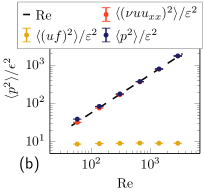
Figure 4: (Color online) (a) The first moment of power, $\langle p\rangle$, is equal to zero. Note how forcing and dissipation exactly cancel each other. (b) The second moment of power, $\langle p^{2}\rangle$, scales like $\mathrm{Re}$. The dissipative term dominates the forcing term.

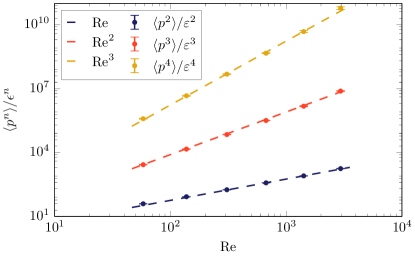
Figure 5: (Color online) Higher moments of power, $\langle p^{n}\rangle$, scale like $\mathrm{Re}^{n-1}$.

In this section we explore a measure of irreversibility that is a direct consequence of the existence of an energy cascade. We consider $\langle p^{3}\rangle=\langle\left(\frac{dE}{dt}\right)^{3}\rangle$ which for a time-reversible system would be equal to zero. Note that the first moment, $\langle p\rangle=0$, due to the balance between dissipation and forcing. For white in time forcing such quantities are ill defined as they correspond to time derivatives at $t=0$. We therefore use forcing with a finite correlation time in the numerical simulations presented here.

To obtain a prediction for the scaling of $\langle p^{n}\rangle$ with the $\mathrm{Re}$ we will use a dimensional reasoning of sorts. First, in general, we can use the Burgers equation to write

$$\left<p^{n}\right>=\left<\left(v\frac{dv}{dt}\right)^{n}\right>=\left<\left[v\left(f+\nu v_{xx}\right)\right]^{n}\right>.$$ (7)

Now, any average including $\nu vv_{xx}$ is concentrated on the shock locations (or places with very large gradients for finite viscosity). These are small regions of thickness of $\nu/v_{rms}$ where the velocity spatial gradient is proportional to $v_{rms}^{2}/\nu$. Thus, for $n\geq 2$ terms including the forcing are sub-dominant to $\langle\left(\nu vv_{xx}\right)^{n}\rangle$ by at least one factor of Reynolds number, $\mathrm{Re}=v_{rms}L/\nu\propto\epsilon^{1/3}L^{4/3}/\nu$. In particular

$$\left<p^{n}\right>\approx\left<\left(\nu vv_{xx}\right)^{n}\right>\propto\frac{1}{L}\nu^{n}\left(\frac{v_{rms}^{4}}{\nu^{2}}\right)^{n}\frac{\nu}{v_{rms}}\propto\epsilon^{n}\mathrm{Re}^{n-1}.$$ (8)

These dimensional estimates, coinciding with the predictions of the “flight-crash” model, are supported by numerical experiments. For the first moment, as shown in figure 4 (left), the forcing and dissipation terms cancel each other. Figure 4 (right) depicts the scaling of the second moment of power, $\langle p^{2}\rangle$ proportional to $\mathrm{Re}$. Note also that the dissipative term, $\langle\left(\nu vv_{xx}\right)^{2}\rangle$ dominates the forcing term $\langle\left(vf\right)^{2}\rangle$, the latter being unaffected by changes in $\mathrm{Re}$. This is a very different situation from that in 2d and 3d incompressible turbulence, where the leading $\mathrm{Re}$ dependence of the power comes from pressure terms. As shown in figure 5, the second to fourth moment of power scale like $\mathrm{Re}^{n-1}$, in accordance with the dimensional estimate of (8).

VI Lagrangian velocity increments

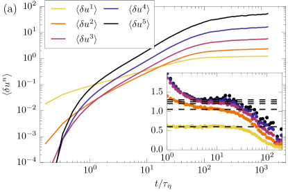
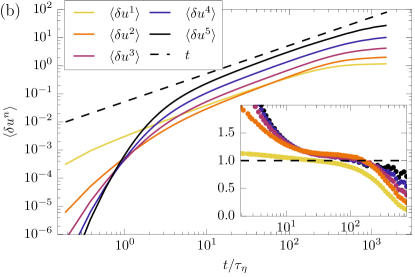
Figure 6: (Color online) Lagrangian velocity increments for white in time forcing (a) and finite forcing correlation time (b), the corresponding local slopes are presented in the respective insets. For the white in time forcing the exponents from Table 1 are marked by dashed lines

As the velocity statistics are non-stationary one may expect to be able to determine the direction of time from the sign of odd moments of velocity differences. In fact, this is not possible since such odd moments are zero: using the invariance of the system under space reflection $\left<(u(t;x_{0})-u(0;x_{0}))^{n}\right>=(-1)^{n}\left<(u(t;-x_{0})-u(0;-x_{0}))^{n}\right>$, and the independence of the average on $x_{0}$, the initial particles position, completes the proof. Of course, non-stationary statistics imply that already the even moments behave differently for positive and negative times ($t=0$ corresponding to a homogeneous particle distribution). In particular backward in times velocity differences are determined solely by the forcing, as particles do not encounter shocks. On the other hand, as we will show, shocks provide a significant contribution forward in time.

The dependence on time of $\left<\left|u(t)-u(0)\right|^{n}\right>=\left<\delta u^{n}\right>$ can be deduced similarly to that of Eulerian velocity differences in this system. There are two competing time scalings which imply bi-fractality. Events where particles do not fall into shocks, which occur with probability $O(1)$, change their velocity diffusively or ballistically depending on whether the forcing is short or finite correlated in time. This gives $\delta u^{n}\propto t^{n}$ for finitely correlated and $\delta u^{n}\propto t^{n/2}$ for delta correlated forcing. On the other hand there are the events where particles fall into shocks, the probability for which scales linearly with time and where the velocity difference is $\delta u^{n}\propto O(1)$. This implies that for times $\tau_{\eta}\ll t\ll T_{L}$, for white in time forcing we expect

$$\left<\delta u^{n}\right>\propto\left\{\begin{array}[]{ll}t^{n/2}&,n<2\\ t&,n\geq 2\end{array}\right.$$

while for forcing with a finite correlation time

$$\left<\delta u^{n}\right>\propto\left\{\begin{array}[]{ll}t^{n}&,n<1\\ t&,n\geq 1.\end{array}\right.$$

Figure 6 shows the results from numerical simulations, for the forcing correlated both short and long in time, largely agreeing with the prediction above. The measured local slopes $d\ln\langle\delta u^{n}\rangle/d\ln t$ are presented in the inset. As a guidance for the eye, we have marked the approximate scaling exponents in the inset of Figure 6 for the white in time forcing. Their values are summarised in Table 1. For the long correlated forcing, although the local slopes are close to $1$, there are no clear plateaus, possibly due to a longer influence of the dynamics at $t\approx\tau_{\eta}$ on the inertial range.

The deviations of the measured local slopes from our prediction apparent in Table 1 and Figure 6 are probably a finite $Re$ effect as well – in the inertial range both competing time scalings are present for all $n$, a single scaling becoming dominant only in the limit $Re\to\infty$. Indeed, the best agreement is observed for $n$ where the two terms are of the same order: $n=1$ for long correlated forcing and $n=2$ for white in time forcing. This would also explain why the white in time local slopes are further from the prediction than the long correlated ones, the two competing terms being closer to each other for the former.

It is worth noting that $\zeta_{2}=1$ is also the prediction for incompressible turbulence in 2d and 3d obtained by dimensional arguments or the multi-fractal phenomenology Biferale2004 ; BoffetaMazzino2008 . Such a relation, however, was never clearly observed either numerically or experimentally falkovich-etal:2012 ; BoffetaMazzino2008 . For the Burgers equation it can also be derived on dimensional grounds, as well as by using the Lagrangian multi-fractal phenomenology. The latter relates the Eulerian scaling to the Lagrangian one by assuming that the time elapsed can be related to the distance travelled via $t\propto r/\delta_{r}u$ and that $\delta u(t)\propto\delta_{r}u$ where $\delta_{r}u=v(r,t)-v(0,t)$ is the Eulerian velocity difference. Then it is predicted that $\zeta_{n}=\min\limits_{h}\left[\frac{nh-D(h)+d}{1-h}\right]$ with $D(h)$ the Eulerian fractal dimension.

For the Burgers equation on shocks $h=0$, $D(0)=0$ and everywhere else $h=1$, $D(1)=1$, which gives the correct prediction for $n\geq 2$. Indeed, the above assumptions are satisfied for the Burgers equation for $n\geq 2$ as shock events control the statistics: due to the presence of the shock $\delta u(t)\propto\delta_{r}u\propto O(1)$ and since the particle moves ballistically relative to the shock $t\propto r$. For $n<2$ while $\delta u(t)\propto\delta_{r}u$ the Eulerian velocity difference tells nothing about the distance travelled $r$, as demonstrated by the dependence of $\zeta_{1}$ on the temporal correlation of the forcing.

For incompressible turbulence, while the Lagrangian multi-fractal phenomenology leads to a good fit in 3d Arneodo2008 ; toschi2009 ; bec-bitane2013 , the assumption $t\propto r/\delta_{r}u$ cannot be universally exact KampsFriedrich2009 . In particular, thinking of averages as a weighted sum over events, different events may dominate the average depending on the quantity one considers, and while the relation $t\propto r/\delta_{r}u$ may work well for some events it can fail for others. Indeed, to obtain the scaling of the energy difference, dominated by flight crash events, $t\propto r$ and $\delta u(t)\propto\delta_{r}u$ were used in xu-pumir-etal:2014 . An elegant way to amplify these same events was recently introduced in LevequeNaso2014 where new longitudinal Lagrangian velocity increments were defined and measured instead of energy differences, revealing that the projection on the direction is the main ingredient. Then, assuming $t\propto r$ and $\delta u(t)_{L}\propto\delta_{r}u$ implies that the Eulerian and longitudinal Lagrangian velocity moments should have the same scaling exponents. This was verified for the third and second order velocity moments in LevequeNaso2014 . It is however unclear why the assumption $t\propto r$ should hold. In this context our observations for the Burgers turbulence may provide some insight: if the change in the particles velocity is due to transition at time $t$ into a region with a different velocity scaling then the distance travelled should be determined by the relative velocity between the two regions, i.e $t\propto r/\delta_{r}u$. On the other hand, the distance travelled by a particle within a region with a single scaling is detached from $\delta_{r}u$.

$p$	1	2	3	4	5
$\zeta_{p}^{\text{white}}$	0.6	1.05	1.2	1.25	1.3

Table 1: Scaling exponents of Lagrangian velocity increments for white in time forcing.

VII Long time statistics

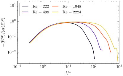
Figure 7: (Color online) Single particle statistics for long times. Again, $-\langle W^{3}\rangle\propto\epsilon t$.

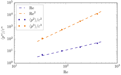
Figure 8: (Color online) The moments of power, $\langle p^{n}\rangle$, for single particle statistics for long times. We recover the scaling $\langle p^{n}\rangle\sim\textrm{Re}^{n-1}$.

As long as the Lagrangian velocity statistics, starting from a homogeneous distribution of particles initially, do not reach a steady state, the irreversibility of the system cannot be attributed solely to the existence of an energy cascade. It is this somewhat trivial component of the irreversible dynamics which we wish to eliminate when considering long time statistics. For long times, all particles accumulate inside shocks, and since any two shocks eventually merge, for very long times, all particles reach the same position in the same shock. Therefore, observing long time statistics is equivalent to considering only a single particle in the entire flow. As new shocks are created with time and, in the spirit of our considerations in the previous sections, we expect the main contribution to come from shock collisions, particle statistics in this regime can also be seen as shock-interaction statistics. We we will perform similar measurements for particles as above, this time arbitrarily defining some $t=0$ when stationary particle statistics are reached, instead of starting with a homogeneous particle density. In contrast to the short-time case it is much harder to obtain good statistics, since the flow is only sampled at a single particle position. We therefore resort to the more robust method of estimating the moments of power $\langle p^{n}\rangle$ by finding the plateau of $\langle W^{n}(t)\rangle/t^{n}$ for short times, instead of evaluating $\langle dE/dt\rangle$ directly. We furthermore restrict the range of $\mathrm{Re}$ to lower values for the power statistics, as obtaining converging results for higher $\mathrm{Re}$ becomes prohibitive. Reaching stationary statistics implies in particular $\langle W\rangle=0$, which we indeed observe. We obtain that $\langle W^{3}\rangle<0$, depicted in figure 7. It turns out that the scaling is very similar to that at short times, with $\langle W^{n}\rangle\propto t$ and $\langle p^{n}\rangle\propto\mathrm{Re}^{n-1}$. The corresponding results from numerical simulations are shown in figure 8 for the second and third moment of power.

We believe that a qualitative explanation for this behavior can be given in terms of shock collisions. Shock collisions are rare events, where the velocity of a given shock is changed by an order one factor. Between such events the shock slowly changes its velocity due to the forcing. In this sense we recover again a “flight-crash” picture: The linear scaling with $t$ of $\langle W^{n}\rangle$ is due to the probability for a shock collision. It is proportional to the probability to encounter a shock during time $t$, which scales like $t$. The scaling of the power moments can then again be derived by matching the scaling of $\left<W^{n}\right>$ for times $t\leq\tau_{\eta}$ and $t\geq\tau_{\eta}$ at $t=\tau_{\eta}$. We note that not every shock collision results in an energy loss. Energy must be lost on average though in order to balance the energy gain from forcing and obtain the stationary state $\left<W\right>=0$.

VIII Conclusion

We have studied time-irreversibility as deduced from the statistics of a single element, a fluid marker, in a compressible turbulent flow. Transferring the ideas of Xu et al. xu-pumir-etal:2014 to Burgers turbulence, we measured Lagrangian energy differences and instantaneous power statistics, and demonstrated the ability of the “flight-crash” model, suggested therein, to explain our results. From the point of view of particles, compressibility itself introduces an additional element of time-irreversibility in the form of shock structures. Therefore, we consider two different regimes: First we consider the trajectory of a particle starting at a random position. Here, we estimate the scaling $\langle W(t)^{n}\rangle\propto t$ and $\langle p^{n}\rangle\propto\textrm{Re}^{n-1}$ by invoking a steady-state shock model. Our numerical simulations confirm these predictions for the form and the pre-factor of $\langle W(t)\rangle$ as well as the general scaling of $\langle W(t)^{n}\rangle$ and $\langle p^{n}\rangle$. Secondly, we examine long-time statistics, where all particles have accumulated in shocks. This regime can be interpreted as shock-interaction statistics. The “flight-crash” picture then applies to the motion of shocks themselves, as they gain energy slowly until hitting another shock, leading to a rapid loss of energy on average. These considerations are again backed by numerical simulations, consistent with $\langle W^{n}(t)\rangle\propto t$ and $\langle p^{n}\rangle\propto\textrm{Re}^{n-1}$.

References

- (1) H. Xu, A. Pumir, G. Falkovich, E. Bodenschatz, M. Shats, H. Xia, N. Francois, and G. Boffetta. Flight–crash events in turbulence. Proceedings of the National Academy of Sciences, 111(21):7558–7563, 2014.
- (2) L. Onsager. Reciprocal relations in irreversible processes. I. Physical Review, 37(4):405–426, February 1931.
- (3) U. Frisch. Turbulence. Cambridge University Press, Cambridge, 1995.
- (4) M. Bauer and D. Bernard. Sailing the deep blue sea of decaying burgers turbulence. Journal of Physics A: Mathematical and General, 32(28):5179, July 1999.
- (5) G. L. Eyink and T. D. Drivas. Spontaneous stochasticity and anomalous dissipation for burgers equation. arXiv:1401.5541 [math-ph, physics:physics], January 2014. arXiv: 1401.5541.
- (6) G. Falkovich, H. Xu, A. Pumir, E. Bodenschatz, L. Biferale, G. Boffetta, A. S. Lanotte, and F. Toschi. On Lagrangian single-particle statistics. Physics of Fluids (1994-present), 24(5):055102, May 2012.
- (7) C. Beetz, C. Schwarz, J. Dreher, and R. Grauer. Density-PDFs and Lagrangian statistics of highly compressible turbulence. Physics Letters A, 372(17):3037–3041, April 2008.
- (8) J. Bec and K. Khanin. Burgers turbulence. Physics Reports, 447(1):1–66, 2007.
- (9) J. M. Burgers. The Nonlinear Diffusion Equation. Asymptotic Solutions and Statistical Problems. Reidel, Dordrecht, 1974.
- (10) R. L. Honeycutt. Stochastic Runge-Kutta algorithms. I. White noise. Physical Review A, 45(2):600–603, January 1992.
- (11) V. Eswaran and S. B. Pope. An examination of forcing in direct numerical simulations of turbulence. Computers & Fluids, 16(3):257–278, 1988.
- (12) CUDA toolkit documentation, 2014. http://docs.nvidia.com/cuda/index.html.
- (13) A. Frishman and G. Falkovich. New type of anomaly in turbulence. Phys. Rev. Lett., 113:024501, Jul 2014.
- (14) G. Falkovich. Fluid mechanics: A short course for physicists. Cambridge University Press, 2011.
- (15) W. E and E. Vanden-Eijnden. Statistical theory for the stochastic Burgers equation in the inviscid limit. Communications on Pure and Applied Mathematics, 53(7):852–901, 2000.
- (16) L. Biferale, G. Boffetta, A. Celani, B. J. Devenish, A. Lanotte, and F. Toschi. Multifractal statistics of lagrangian velocity and acceleration in turbulence. Phys. Rev. Lett., 93:064502, Aug 2004.
- (17) G. Boffetta, A. Mazzino, and A. Vulpiani. Twenty-five years of multifractals in fully developed turbulence: a tribute to giovanni paladin. Journal of Physics A: Mathematical and Theoretical, 41(36):363001, 2008.
- (18) A. Arnèodo, R. Benzi, J. Berg, L. Biferale, E. Bodenschatz, A. Busse, E. Calzavarini, B. Castaing, M. Cencini, L. Chevillard, T. Fisher, R. R. Grauer, H. Homann, D. Lamb, A. S. Lanotte, E. Lévèque, B. Lüthi, J. Mann, N. Mordant, W.-C. Müller, S. Ott, N. T. Ouellette, J.-F. Pinton, S. B. Pope, S. G. Roux, F. Toschi, H. Xu, and P. K. Yeung. Universal intermittent properties of particle trajectories in highly turbulent flows. Phys. Rev. Lett., 100:254504, Jun 2008.
- (19) F. Toschi and E. Bodenschatz. Lagrangian properties of particles in turbulence. Annual Review of Fluid Mechanics, 41(1):375–404, 2009.
- (20) R. Bitane, H. Homann, and J. Bec. Geometry and violent events in turbulent pair dispersion. Journal of Turbulence, 14(2):23–45, 2013.
- (21) O. Kamps, R. Friedrich, and R. Grauer. Exact relation between eulerian and lagrangian velocity increment statistics. Phys. Rev. E, 79:066301, Jun 2009.
- (22) E. Leveque and A. Naso. Introduction of longitudinal and transverse lagrangian velocity increments in homogeneous and isotropic turbulence. EPL (Europhysics Letters), 108(5):54004, 2014.