Exact solutions of three dimensional black holes:
Einstein gravity vs $F(R)$ gravity

Abstract

In this paper, we consider Einstein gravity in the presence of a class of nonlinear electrodynamics, called power Maxwell invariant (PMI). We take into account $(2+1)$-dimensional spacetime in Einstein-PMI gravity and obtain its black hole solutions. Then, we regard pure $F(R)$ gravity as well as $F(R)$-conformally invariant Maxwell theory to obtain exact solutions of the field equations with black hole interpretation. Finally, we investigate the conserved and thermodynamic quantities and discuss about the first law of thermodynamics for the mentioned gravitational models.

I introduction

In recent years, the luminosity distance of Supernovae type Ia Perlmutter , wide surveys on galaxies Gal and the anisotropy of cosmic microwave background radiation CMBR confirm that the expansion of our Universe is currently undergoing a period of acceleration. Large scale structure formation LSS , baryon oscillations BO and weak lensing WL also suggest such an accelerated expansion of the Universe. Identifying the cause of this late time acceleration is one of the most challenging problems of modern cosmology. Theoretical physicists desire to interpret this accelerated expansion in a suitable gravitational background and they proposed some candidates. A positive cosmological constant can lead to accelerated expansion of the universe but it is plagued by the fine tuning problem Copeland . The cosmological constant may be interpreted either geometrically as modifying the left hand side of Einstein’s equation or as a kinematic term on the right hand side with the equation of state parameter $w=-1$. Another approach can further be generalized by considering a source term with an equation of state parameter $w<-1/3$. Such kinds of source terms have collectively come to be known as Dark Energy. Various scalar field models of dark energy have been considered in literature Armendariz . All the dark energy based theories assume that the observed acceleration is the outcome of the action of a still unknown ingredient added to the cosmic pie. In terms of the Einstein equations, such models are simply modifying the right hand side including in the stress–energy tensor with something more than the usual matter and radiation components.

On the other hand, one can also try to leave unchanged the source side, but rather than modifying the left hand side of Einstein field equations. In a sense, one is therefore interpreting cosmic acceleration as a first signal of the breakdown of the laws of physics as described by the standard General Relativity (GR). There are different branches of modified gravity with various motivations. Lovelock gravity Lovelock , brane world cosmology Gergely , scalar-tensor theories Jordan and also the so-called $F(R)$ gravity FR ; HendiGRG ; HendiPRD are some of modified gravity theories.

Modifying GR, not simply given its positive results, opens the way to a large class of alternative theories of gravity ranging from extra dimensions Dvali to non-minimally coupled scalar fields Caresia . In particular, we will be interested here in fourth order theories Capozziello based on replacing the scalar curvature R in the Hilbert–Einstein action with a generic analytic function F(R) which should be reconstructed starting from data and physically motivated issues.

In this paper we are interested in $F(R)$ gravity. But as we know the field equations of $F(R)$ gravity are complicated fourth-order differential equations, and it is not easy to find exact analytical solutions. In addition, adding stress-tensor of a matter field to $F(R)$ gravity, increase its difficulties. Recently, it has been shown that one can extract exact analytical solutions of $F(R)$ theory coupled to a traceless energy momentum tensor with constant curvature scalar Moon . For example, taking into account the conformally invariant Maxwell (CIM) field as a matter source, which is traceless in arbitrary dimensions, some black objects of $F(R)$ gravity were obtained in higher dimensions Sheykhi .

On the other hand, one of the interesting subjects for recent study is the investigation of three dimensional black holes Hodgkinson . Taking into account three dimensional solutions helps us to find a profound insight in the black hole physics, quantum view of gravity and also its relations to string theory Carlip ; Witten . Moreover, three dimensional spacetimes perform an essential role to improve our understanding of gravitational interaction in low dimensional manifolds Witten2007 . Due to these facts, some of physicists have an interest in the $(2+1)$-dimensional manifolds and their attractive properties BTZ ; Nojiri1998 . Although three dimensional black holes in $F(R)$ gravity have been studied before ThreeF(R) ; HendiIJPT , till now, exact solution of three dimensional $F(R)$ gravity coupled to a matter field have not been constructed. In this paper, one of our goals is obtaining an exact three dimensional black hole solutions of $F(R)$ theory coupled to a CIM source.

The coupling of nonlinear sources and general relativity attract the significant attentions because of their specific properties. Interesting properties of various nonlinear electrodynamics have been studied before NLED . One of the special class of the nonlinear electrodynamics sources is PMI, which its Lagrangian is an arbitrary power of Maxwell Lagrangian Hassaine2008 . This Model is considerably richer than Maxwell theory and in the special case (unit power), it reduces to linear Maxwell field. Another attractive feature of the PMI theory is its conformal invariance when the power of Maxwell invariant is a quarter of spacetime dimensions. In other words, for the special choice $power=dimensions/4$, one obtains traceless energy-momentum tensor which leads to conformal invariance. It is notable that the idea is to take advantage of the conformal symmetry to construct the analogues of the four dimensional Reissner-Nordström solutions with an inverse square electric field in arbitrary dimensions Hassaine2007 .

Recently it has been shown that one can, simultaneously, extract electric charge and cosmological constant from pure $F(R)$ gravity (without matter field: $T_{\mu\nu}=0$) HendiGRG . Another goal of this paper is obtaining three dimensional charged black hole solutions from pure $F(R)$ gravity as well as $F(R)$-CIM gravity and compare them.

The outline of our paper is as follows. In Sec. II, we review three dimensional black hole solutions in Einstein-Maxwell gravity. Then we investigate the black hole solutions of Einstein-PMI and Einstein-CIM theories. Sec. III is devoted to obtain black hole solutions of pure $F(R)$ gravity as well as $F(R)$-CIM theory and compare these solutions. In Sec. IV, we discuss about the conserved and thermodynamic quantities of the solutions and check the first law of thermodynamics. We terminate our paper by some conclusions.

II Three dimensional solutions in Einstein gravity

II.1 Brief review of Einstein-Maxwell solutions

The charged BTZ black hole is the solution of the $(2+1)$-dimensional Einstein-Maxwell gravity with a negative cosmological constant $\Lambda=-\frac{1}{l^{2}}$ BTZ2000 . The line element can be written as

$$ds^{2}=-g(r)dt^{2}+\frac{dr^{2}}{g(r)}+r^{2}d\varphi^{2},$$ (1)

where the metric function is

$$g(r)=\frac{r^{2}}{l^{2}}-m-2q^{2}\ln(\frac{r}{l}),$$ (2)

where $m$ and $q$ are the mass and the electric charge of the black hole, respectively.

Here, we want to review the geometrical structure of this solution, briefly. We first look for the essential singularity(ies). The Ricci scalar and the Kretschmann scalar can be written in the following form

$$R = \frac{2\left(q^{2}l^{2}-3r^{2}\right)}{r^{2}l^{2}},$$ (3)

$$R_{\alpha\beta\mu\nu}R^{\alpha\beta\mu\nu} = \frac{4\left(3r^{4}-2r^{2}q^{2}l^{2}+3q^{4}l^{4}\right)}{r^{4}l^{4}},$$ (4)

which indicate that

$$\lim_{r\longrightarrow 0}R \longrightarrow \infty$$

$$\lim_{r\longrightarrow 0}R_{\alpha\beta\gamma\delta}R^{\alpha\beta\gamma\delta} \longrightarrow \infty,$$ (5)

and so confirm that there is a curvature singularity at $r=0$. Also The Ricci and Kretschmann scalars are $\frac{-6}{l^{2}}$ and $\frac{12}{l^{4}}$ at $r\longrightarrow\infty$, and one concludes  that the asymptotic behavior of the charged BTZ black hole is adS. Also we plot $g(r)$ versus $r$ in Fig. 1, to show that the solution (2) may be interpreted as naked singularity or black hole with two horizons or extreme black hole.

Figure 1: $g(r)$ (Eq. (2)) versus $r$ for $l=1$, $q=1$, and $m=0.2$ (dashed line), $m_{ext}=0.98$ (bold line) and $m=2.5$ (continuous line).

II.2 Einstein-PMI and Einstein-CIM solutions

Now, we take into account the Einstein gravity in the presence of a matter source in the form $\left(F_{\mu\nu}F^{\mu\nu}\right)^{s}$, so called Einstein-PMI gravity Hassaine2008 . Black hole solutions in $(n+1)$-dimension of Einstein-PMI gravity have been studied before HendiEPJC2011 for spacial value of $s$. Here, we want to focus on the $(2+1)$-dimension of Einstein-PMI gravity for arbitrary $s$ and discuss about the properties of the solutions. The $(2+1)$-dimensional action in which gravity is coupled to nonlinear electrodynamics in the presence of negative cosmological constant may be written as HendiEPJC2011

$$I~{}\left(g_{\mu\nu},~{}A_{\mu}\right)=\frac{1}{16\pi}\int_{\partial M}d^{3}x\sqrt{-g}\left[R-2\Lambda+\left(\kappa F\right)^{s}\right],$$ (6)

where $R$ is the scalar curvature, $F$ is the Maxwell invariant which is equal to $F_{\mu\nu}F^{\mu\nu}$ (where $F_{\mu\nu}=\partial_{\mu}A_{\nu}-\partial_{\nu}A_{\mu}$ is the electromagnetic tensor field and $A_{\mu}$ is the gauge potential), and $s$ is an arbitrary positive nonlinearity parameter ($s\neq\frac{1}{2}$). Varying the action (6) with respect to the metric tensor $g_{\mu\nu}$ and the electromagnetic field $A_{\mu}$, the equations of gravitational and electromagnetic fields may be obtained as

$$G_{\mu\nu}-\Lambda g_{\mu\nu}=T_{\mu\nu},$$ (7)

$$\partial_{\mu}\left(\sqrt{-g}F^{\mu\nu}\left(\kappa F\right)^{s-1}\right)=0,$$ (8)

in which the energy-momentum tensor of Eq. (7) is

$$T_{\mu\nu}=2\left[s\kappa F_{\mu\rho}F_{\nu}^{\rho}\left(\kappa F\right)^{s-1}-\frac{1}{4}g_{\mu\nu}\left(\kappa F\right)^{s}\right],$$ (9)

where $\kappa$ is a constant. It is easy to show that when $s$ and $\kappa$ go to $-1$, Eqs. (6-9), reduce to the field equations of black hole in Einstein-Maxwell gravity. Since the Maxwell invariant is negative, hereafter we set $\kappa=-1$, without loss of generality.

We look for black hole solutions with a radial electric field, so the gauge potential is given by

$$A_{\mu}=h(r)\delta_{\mu}^{0},$$ (10)

where the electromagnetic field equation (8), leads to

$$h(r)=\left\{\begin{array}[]{c}q\ln(\frac{r}{l})\text{ \ \ \ \ \ \ \ }s=1\\ -qr^{\left(\frac{2(s-1)}{2s-1}\right)}\text{ \ \ \ \ \ \ \ }otherwise\end{array}\right.,$$ (11)

where $q$ is an integration constant related to electric charge. It is easy to show that the only nonzero electromagnetic field tensor is

$$F_{tr}=\left\{\begin{array}[]{c}\frac{q}{r}\text{ \ \ \ \ \ \ \ \ \ \ \ \ }s=1\\ \frac{-2q\left(s-1\right)}{(2s-1)}r^{\frac{-1}{2s-1}}\text{ \ \ }otherwise\end{array}\right..$$ (12)

In order to have asymptotically well-defined electric field, we should restrict the nonlinearity parameter to $s>\frac{1}{2}$.

To find the function $g(r)$, one may use the components of Eq. (7). The simplest equation is the $rr$ (or $tt$) component of this equation which can be written as

$$\left\{\begin{array}[]{c}g^{\prime}(r)+2\Lambda r-\frac{2q^{2}}{r}=0\text{ \ \ \ \ \ \ \ \ \ \ \ \ \ \ \ \ \ \ \ \ \ \ \ \ \ \ \ \ \ \ \ \ \ \ \ \ \ }s=1\\ g^{\prime}(r)+2\Lambda r+r\left(1-2s\right)\left(\frac{8q^{2}r^{\left(\frac{-2}{2s-1}\right)}\left(s-1\right)^{2}}{\left(2s-1\right)^{2}}\right)^{s}=0\text{ \ \ }otherwise\end{array},\right.$$ (13)

with the following solutions

$$g(r)=\frac{r^{2}}{l^{2}}-m+\left\{\begin{array}[]{c}2q^{2}\ln(\frac{r}{l})\text{ \ \ \ \ \ \ \ \ \ \ \ }s=1\\ \frac{\left(2s-1\right)^{2}\left(\frac{8q^{2}\left(s-1\right)^{2}}{\left(2s-1\right)^{2}}\right)^{s}}{2\left(s-1\right)}r^{\left(\frac{2\left(s-1\right)}{2s-1}\right)}\text{ \ }otherwise\end{array},\right.$$ (14)

where $m$ is an integration constant related to mass. We should note that Eq. (14) satisfy all field equations. We should note that since $s>\frac{1}{2}$, the first term of Eq. (14) is dominant term for $r\rightarrow\infty$ and therefore the asymptotic behavior of the solutions is adS. In other word, the nonlinearity does not affect on the asymptotic behavior of the solutions.

Now, we want to investigate the special case $s=\frac{3}{4}$, the so-called conformally invariant Maxwell field. It has been shown that for $s=\frac{d}{4}$ ($d$=spacetime dimension), the energy-momentum tensor will be traceless and the corresponding electric field will be proportional to $r^{-2}$ as it take place for Maxwell field in four dimension. Here, we consider $s=\frac{3}{4}$ (see for more details Hassaine2007 ) into Eqs. (12) and (14) to obtain

$$F_{tr}=\frac{q}{r^{2}},$$ (15)

$$g(r)=\frac{r^{2}}{l^{2}}-m-\frac{\left(2q^{2}\right)^{\frac{3}{4}}}{2r}.$$ (16)

We should note that for $PMI$ solution, the metric function $g(r)$ has one real root (such as uncharged solutions). This behavior take place for the metric function (14), when we choose $s\neq 1$ (see Fig. 2).

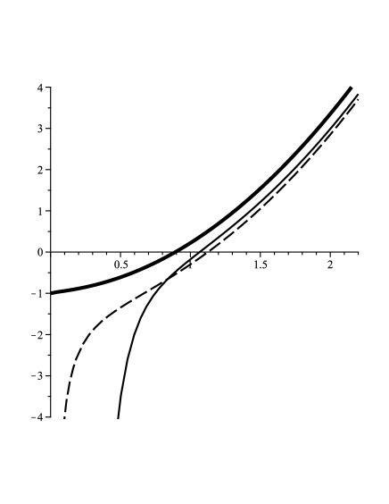
Figure 2: $g(r)$ (Eq. (14)) versus $r$ for $\l=1$, $q=0.5$, $m=1$ and $s=3/4$ (dashed line), $s=2$ (bold line) and $s=3/5$ (continuous line).

III Three dimension solutions in F(R) gravity

III.1 F(R)-CIM solution

In this section, we consider $F(R)$ gravity in the presence the conformally invariant Maxwell field as a source, which leads to traceless energy-momentum tensor.

The equations of motion of $F(R)-CIM$ theory can be written as

$$R_{\mu\nu}\left(1+f_{R}\right)-\frac{1}{2}g_{\mu\nu}F(R)+\left(g_{\mu\nu}\nabla^{2}-\nabla_{\mu}\nabla_{\nu}\right)f_{R}=8\pi\mathrm{T}_{\mu\nu},$$ (17)

$$\partial_{\mu}\left(\sqrt{-g}\frac{F^{\mu\nu}}{\left(-F\right)^{\frac{1}{4}}}\right)=0,$$ (18)

where $f_{R}=\frac{df(R)}{dR}$. It is notable that the assumption of a traceless energy-momentum tensor is essential for deriving exact black hole solutions in $f(R)$ gravity coupled to the matter field in metric formalism.

Now, we want to obtain the solutions for the constant scalar curvature is $R=R_{0}$= const. Using Eq. (10) with (18), we can obtain

$$h(r)=\frac{-\mathcal{Q}}{r},$$ (19)

$$F_{tr}=\frac{\mathcal{Q}}{r^{2}},$$ (20)

The trace of Eq. (17) yields

$$R_{0}\left(1+f_{R}\right)-\frac{3}{2}\left(R_{0}+f(R_{0})\right)=0,$$ (21)

and solving the above equation for $R_{0}$ gives

$$R_{0}=\frac{3f(R_{0})}{2f_{R}-1}\equiv 6\Lambda.$$ (22)

Substituting the above relation into Eq. (17), we obtain the following equation

$$R_{\mu\nu}\left(1+f_{R}\right)-\frac{1}{3}g_{\mu\nu}R_{0}\left(1+f_{R}\right)=8\pi\mathrm{T}_{\mu\nu}.$$ (23)

Considering metric (1) and field equation (23), one can write the following field equations

$$\left[r^{2}\left(2\mathcal{Q}^{2}\right)^{\frac{1}{4}}\left(rg^{\prime\prime}(r)+g^{\prime}(r)+\frac{2}{3}rR_{0}\right)\right]\left(1+f_{R}\right)=-\mathcal{Q}^{2},$$ (24)

$$\left[3g^{\prime}(r)+rR_{0}\right]\left(1+f_{R}\right)=\frac{3}{2r^{2}}\left(2\mathcal{Q}^{2}\right)^{\frac{3}{4}},$$ (25)

corresponding to $tt\$(or $rr$) and $\varphi\varphi$ components, respectively. After some calculations, one can obtain the following metric function

$$g(r)=-m-\frac{\left(2\mathcal{Q}^{2}\right)^{\frac{3}{4}}}{2\left(1+f_{R}\right)r}-\frac{r^{2}R_{0}}{6},$$ (26)

where we restrict ourselves to $f^{\prime}(R_{0})\neq-1$. We want to study the general structure of the solutions. One can find that the Kretschmann scalar is

$$R_{\alpha\beta\gamma\delta}R^{\alpha\beta\gamma\delta}=\frac{2r^{6}R_{0}^{2}\left(1+f_{R}\right)^{2}+9(2\mathcal{Q}^{2})^{\frac{3}{2}}}{6r^{6}\left(1+f_{R}\right)^{2}},$$ (27)

where confirms that the Kretschmann scalar diverges at $r=0$, is finite for $r\neq 0$, and is proportional to $\frac{R_{0}^{2}}{3}$ as $r\longrightarrow\infty$. Therefore, there is a curvature singularity located at $r=0$ and the spacetime is asymptotically adS provided we define $R_{0}=-\frac{6}{l^{2}}$. In order to have physical solutions we should restrict ourselves to $f_{R}\neq-1$. For $f_{R}>-1$, one can substitute $R_{0}$ and $\mathcal{Q}$ with $-\frac{6}{l^{2}}$ and $q[1+f_{R}]^{\frac{2}{3}}$, respectively to obtain the metric function of Einstein-$CIM$ gravity (16) with one non-extreme root (such as Schwarzschild black hole).

III.2 Pure $F(R)$ gravity solutions

Here, we are looking for charged solutions of pure $F(R)$ gravity. We consider $F(R)=R+f(R)$ gravity without matter field ($\mathrm{T}_{\mu\nu}^{matt}=0$) in $(2+1)$-dimension.

Considering metric (1) and field equation (17), one can obtain the following independent sourceless equations HendiIJPT

$$2rg(r)F_{R}^{\prime\prime}+\left[rg^{\prime}(r)+2g(r)\right]F_{R}^{\prime}-\left[rg^{\prime\prime}(r)+g^{\prime}(r)\right]F_{R}=rF(R),$$ (28)

$$\left[rg^{\prime}(r)+2g(r)\right]F_{R}^{\prime}-\left[rg^{\prime\prime}(r)+g^{\prime}(r)\right]F_{R}=rF(R),$$ (29)

$$2rg(r)F_{R}^{\prime\prime}+2g^{\prime}(r)\left[rF_{R}^{\prime}-F_{R}\right]=rF(R),$$ (30)

corresponding to $tt$, $rr$ and $\varphi\varphi$ components, respectively. In these equation $F_{R}=\frac{dF(R)}{dR}$ and prime denotes derivative with respect to $r$. In this paper, we study black hole solutions with constant Ricci scalar (so $F_{R}^{\prime\prime}=F_{R}^{\prime}=0$) , therefore it is easy to show that the field Eqs. (28)-(30) reduce to

$$\left[rg^{\prime\prime}(r)+g^{\prime}(r)\right]F_{R} = -rF(R),$$ (31)

$$2g^{\prime}(r)F_{R} = -rF(R).$$ (32)

Hereafter, we should choose a model of $f(R)$ to obtain exact solution. To find the function $g(r)$, we use the components of Eqs . (31) and (32) with well-known $F(R)=R-\lambda\exp(-\xi R)+\eta R^{n}$ model. Using of Eqs. (31) and (32) with metric (1), one can obtain a general solution in the following form

$$g(r)=\frac{r^{2}}{l^{2}}-m+\frac{K}{r},$$ (33)

where $K$ is integration constants. In order to satisfy all components of the field equation, we should set the parameters of the $F(R)$ model such that satisfy the following equations

$$R\left(\eta(2n-3)R^{n-1}-1\right)e^{\xi R}+\lambda\left(3+2\xi R\right)=0,$$ (34)

$$\eta nR\left(R^{n-1}-1\right)e^{\xi R}-6\lambda\xi=0.$$ (35)

Solving Eqs. (34) and (35) for $\lambda$ and $\eta$ with arbitrary $\xi$ lead to the following solutions

$$\eta=\frac{-\left(1+\xi R\right)}{R^{n-1}\left(n+\xi R\right)},$$ (36)

$$\lambda=\frac{6e^{\xi R}\left(n-1\right)}{n+\xi R}.$$ (37)

The solution (33) known as uncharged BTZ black hole solution, when $K=0$ BTZ . Calculations show that the Kretschmann scalar is in the following form

$$R_{\alpha\beta\mu\nu}R^{\alpha\beta\mu\nu}=\frac{6\left(2r^{6}+K^{2}l^{4}\right)}{r^{6}l^{4}}$$ (38)

which confirms that

$$\lim_{r\longrightarrow 0}R_{\alpha\beta\gamma\delta}R^{\alpha\beta\gamma\delta}\longrightarrow\infty,$$ (39)

and so there is a singularity at $r=0$. Also, the Kretschmann scalar is $\frac{12}{l^{4}}$ for $r\longrightarrow\infty$ and so asymptotic behavior of the mentioned spacetime is similar to charged adS BTZ black holes. On the other hand, comparing the solution (33) with the solution (26) that shows that these solutions are the same provided $K=$ $-\frac{\left(2\mathcal{Q}^{2}\right)^{\frac{3}{4}}}{2\left(1+f^{\prime}(R_{0})\right)}$ and $l^{2}=\frac{-6}{R_{0}^{2}}$. In other words, one can extract charged solution of pure gravity provided the parameter of the solution (33) is chosen suitably. Also we plot $g(r)$ versus $r$ in Fig. 3, and find that the presented solutions may be interpreted as black hole solutions with two horizons, extreme black hole or naked singularity.

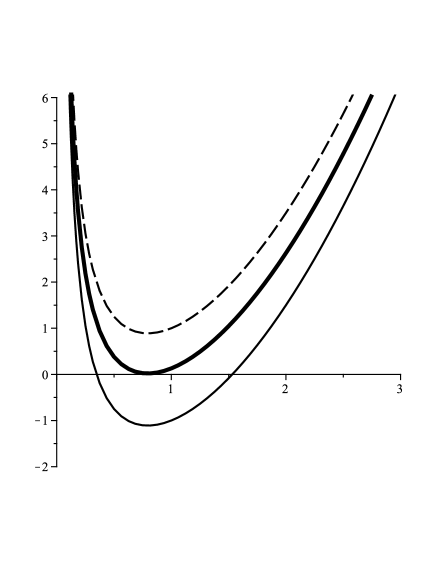
Figure 3: $g(r)$ (Eq. (33)) versus $r$ for $\l=1$, $K=1$, and $m=1$ (dashed line), $m=1.87$ (bold line) and $m=3$ (continuous line).

Choosing an $F(R)$ model, we should discuss about its stability. It was showed that there is no stable ground state for $F(R)$ models if $F(R)\neq 0$ and $F_{R}=0$ Schmidt . For the obtained solutions, we find that $F(R)=F_{R}=0$. Furthermore, it has been shown that $F_{RR}=d^{2}F/dR^{2}$ is related to the the effective mass of the dynamical field of the Ricci scalar Dolgov . Therefore, the positive effective mass, a requirement usually referred to as the Dolgov-Kawasaki stability criterion, leads to the stable dynamical field Faraoni . In order to check the Dolgov-Kawasaki stability criterion, we should calculate the second derivative of the $F(R)$ function with respect to the Ricci scalar for this specific model

$$F_{RR}=-\frac{R(n-1)\left(\xi^{2}+nR^{-2}(1+\xi R)\right)}{n+\xi R},$$ (40)

The positivity of $F_{RR}$ depends on the model parameters. The sign of Eq. (40) is not clear for arbitrary values of parameter. Therefore we plot $F_{RR}$ in Fig. 4 to analyze the sign of $F_{RR}$. This figure shows that one may obtain stable solution for special values of $\xi$ for negative cosmological constant. In other words, we can set free parameters to obtain stable model.

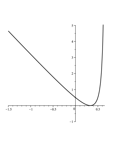
Figure 4: $FRR$ versus $\xi$ for $l=1$, and $n=4$.

IV Thermodynamics

In this section, we calculate the conserved and thermodynamics quantities of the black hole solutions in $(2+1)$-dimension for checking the first law of thermodynamics.

IV.1 Einstein-PMI and Einstein-CIM gravities

The Hawking temperature of the black hole on the outer horizon $r_{+}$, may be obtained through the use of the definition of surface gravity,

$$T_{+}=\frac{1}{2\pi}\sqrt{-\frac{1}{2}\left(\nabla_{\mu}\chi_{\nu}\right)\left(\nabla^{\mu}\chi^{\nu}\right)},$$ (41)

where $\chi=\partial/\partial t$ is the Killing vector. We calculate the Hawking temperature for the PMI black hole solutions, with the following form

$$T_{+}=\left\{\begin{array}[]{c}\frac{1}{2\pi l^{2}}\left(r_{+}-\frac{q^{2}l^{2}}{r_{+}}\right)\text{ \ \ \ \ \ \ \ }s=1\\ \frac{1}{4\pi l^{2}}\left(2r_{+}+\frac{l^{2}\left(2s-1\right)\left(\frac{8q^{2}\left(s-1\right)^{2}}{\left(2s-1\right)^{2}}\right)^{s}}{r_{+}^{\frac{1}{1-2s}}}\right)\text{ \ }otherwise\end{array}\right..$$ (42)

Moreover, we known that the electric potential $U$, measured at infinity with respect to the horizon, is defined by Cvetic

$$U=A_{\mu}\chi^{\mu}\left|{}_{r\rightarrow\infty}\right.-A_{\mu}\chi^{\mu}\left|{}_{r=r_{+}}\right.=\left\{\begin{array}[]{c}-q\ln(\frac{r_{+}}{l})\text{ \ \ \ \ \ \ \ \ \ \ \ }s=1\\ qr_{+}^{\left(\frac{2\left(s-1\right)}{2s-1}\right)}\text{ \ \ \ \ \ \ \ \ }otherwise\end{array}\right..$$ (43)

Usually entropy of the black holes satisfies the so-called area law of entropy which states that the black hole entropy equals to one-quarter of horizon area Beckenstein . Since the area law of the entropy is universal, and applies to all kinds of black holes in Einstein gravity Beckenstein , therefore the entropy of the black holes in $(2+1)$-dimension is equal to one-quarter of the area of the horizon, i.e.,

$$S=\frac{\pi r_{+}}{2}.$$ (44)

In order to calculate the electric charge of the black holes, $Q$, one can obtain the flux of the electromagnetic field at infinity, yielding

$$Q=2^{s-2}\left(\frac{2q\left(s-1\right)}{\left(2s-1\right)}\right)^{2s-1}.$$ (45)

The present spacetime (1), have boundaries with timelike $\left(\xi=\partial/\partial t\right)$ Killing vector field. It is straightforward to show that for the quasi local mass we have

$$M=\frac{m}{8}.$$ (46)

Having conserved and thermodynamic quantities at hand, we are in a position to check the first law of thermodynamics for our solutions. We obtain the mass as a function of the extensive quantities $S$ and $Q$. One may then regard the parameters $S$, and $Q$ as a complete set of extensive parameters for the mass $M(S,Q)$

$$M(S,Q)=\frac{2^{\frac{2-3s}{2s-1}}\left(2s-1\right)^{2}\left(\frac{S}{\pi}\right)^{\frac{2\left(s-1\right)}{2s-1}}Q^{\frac{2s}{2s-1}}+\frac{\left(s-1\right)}{2l^{2}}\left(\frac{S}{\pi}\right)^{2}}{\left(s-1\right)},$$ (47)

we define the intensive parameters conjugate to $S$ and $Q$. These quantities are the temperature and the electric potential

$$T=\left(\frac{\partial M}{\partial S}\right)_{Q}\ \ \ \ ,\ \ \ \ U=\left(\frac{\partial M}{\partial Q}\right)_{S}.$$ (48)

Equations (48) are coincide with Eqs. (42) and (45) and therefore we find that these thermodynamics quantities satisfy the first law of black hole thermodynamics

$$dM=TdS+UdQ.$$ (49)

IV.2 F(R)-CIM gravity

Here, we calculate the Hawking temperature for the black hole solutions of $F(R)$-$CIM$ gravity. Such as previous method, we use the definition of surface gravity to calculate the Hawking temperature. So using Eq. (41) and Eq. (26), we have

$$T_{+}=\frac{r_{+}}{8\pi(1+f_{R})}\left(\frac{\left(2\mathcal{Q}^{2}\right)^{\frac{3}{4}}}{r_{+}^{3}}-\frac{2}{3}R_{0}\left(1+f_{R}\right)\right).$$ (50)

The electric charge of the conformally invariant $F(R)$ black hole can be obtained as

$$Q=\frac{3\mathcal{Q}^{\frac{1}{2}}}{2^{\frac{13}{4}}}.$$ (51)

The electric potential $U$ is Cvetic

$$U=A_{\mu}\chi^{\mu}\left|{}_{r\rightarrow\infty}\right.-A_{\mu}\chi^{\mu}\left|{}_{r=r_{+}}\right.=\frac{\mathcal{Q}}{r_{+}}.$$ (52)

By using the Noether charge method for evaluating the entropy associated with black-hole solutions in $F(R)=R+f(R)$ theory, it was shown that the area law does not hold, and one obtains a modification of the area law Cognola2005

$$S=\frac{A}{4}F_{R},$$ (53)

where $A$ is the horizon area. Hence, we can write

$$S=\frac{\pi r_{+}}{2}\left(1+f_{R}\right),$$ (54)

which shows that the area law does not hold for the black hole solutions in $R+f(R)$ gravity.

Using the same approach, we find that the finite mass can be given by

$$M=\frac{m}{8}\left(1+f_{R}\right).$$ (55)

Having the conserved and thermodynamic quantities of the system at hand, we can check the validity of the first law of black-hole thermodynamics. It is a matter of straightforward calculation to show that the conserved and thermodynamics quantities satisfy the first law of thermodynamics

$$dM=TdS+UdQ.$$ (56)

IV.3 Pure gravity

At first, we investigate the Hawking temperature of the pure black hole on the outer horizon $r_{+}$. It is a matter of calculation to show that

$$T_{+}=\frac{1}{4\pi l^{2}}\left(2r_{+}-\frac{Kl^{2}}{r_{+}^{2}}\right),$$ (57)

which shows that the temperature of the solution is positive definite provided $K>2r_{+}^{3}/l^{2}$.

For the obtained solutions of pure gravity, $F(R)=F_{R}=0$ and therefore using the method of Ref. Cognola2005 , one may encounter with zero entropy. In order to obtain correct nonzero entropy, one may consider the first law as a fundamental principle, i.e.

$$dS=\frac{1}{T}dM.$$ (58)

Using the $\partial/\partial t$ as a Killing vector, one can obtain the following relation for the finite mass

$$M=\frac{m}{8}=\frac{1}{8}\left[\frac{r_{+}^{2}}{l^{2}}+\frac{K}{r_{+}}\right].$$ (59)

Hence, we can write

$$dM=\frac{1}{8}\left[\frac{2r_{+}}{l^{2}}-\frac{K}{r_{+}^{2}}\right]dr_{+},$$ (60)

to calculate the entropy as follows

$$S=\int\frac{1}{T}dM=\int\frac{1}{\frac{-1}{4\pi}\left(\frac{K}{r_{+}^{2}}-\frac{2r_{+}}{l^{2}}\right)}\frac{\frac{2r_{+}}{l^{2}}-\frac{K}{r_{+}^{2}}}{8}dr_{+},$$ (61)

$$S=\frac{\pi}{2}\int dr_{+}=\frac{\pi r_{+}}{2},$$ (62)

which is nothing but the are a law for the entropy. In other words, considering the $F(R)$ gravity with $F_{R}=0$, one may use the the so-called area law instead of modified area law Cognola2005 .

V Conclusions

In this paper, we regarded some various gravitational theories in $(2+1)$ dimensions. At first, we reviewed the Einstein-Maxwell gravity and then we considered Einstein-PMI and Einstein-CIM theories. We obtained the black hole solutions of these theories and studied their properties. We showed that the black holes of the mentioned nonlinear electrodynamics covered with one horizon such as uncharged (Schwarzschild) black holes.

After that, we took into account the pure $F(R)$ gravity as well as $F(R)$-CIM theory to obtain the black hole solutions. We showed that for the pure gravity, one can extract the electrical charge and cosmological constant, simultaneously. In addition, we showed that the asymptotic behavior of obtained solutions is adS.

Finally, we computed the conserved and thermodynamics quantities of the black hole solutions in $(2+1)$-dimension for various theories and found that they satisfy the first law of thermodynamics. In other words, regarding the pure $F(R)$ gravity, we considered the first law as a fundamental principle and proposed that despite the modified area law of entropy ($S=\frac{A}{4}F_{R}$) being true for $F_{R}\neq 0$ model, but we should regard the area law for $F_{R}=0$ cases.

In this paper, we only considered static three dimensional spacetime. Therefore it is worthwhile to think about the cosmological scenario by regarding time dependent spacetime with exact solutions of equations of motion depending on time. One more subject of interest for further study is finding the corresponding scalar-tensor gravity solutions and these subjects are under examination.

- (1) A. G. Riess et al., Astron. J. 116, 1009 (1998); S. Perlmutter et al., Astrophys. J. 517, 565 (1999); A. G. Riess et al., Astrophys. J. 607, 665 (2004).
- (2) S. Cole et al., Mon. Not. Roy. Astron. Soc. 362, 505 (2005).
- (3) D. N. Spergel et al., [WMAP collaboration], Astrophys. J. Suppl. 170, 377 (2007).
- (4) U. Seljak et al., [SDSS collboration], Phys. Rev. D 71, 103515 (2005).
- (5) D. J. Eisenstein et al., [SDSS collboration], Astrophys. J. 633, 560 (2005).
- (6) B. Jain and A. Taylor, Phys. Rev. Lett. 91, 141302 (2003).
- (7) V. Sahni and A. A. Starobinsky, Int. J. Mod. Phys. D 9, 373 (2000); T. Padmanabhan, Phys. Rep. 380, 235 (2003); E. J. Copeland, M. Sami and S. Tsujikawa, Int. J. Mod. Phys. D 15, 1753 (2006); E. V. Linder, Gen. Relativ. Gravit. 40, 329 (2008); J. Frieman, M. Turner and D. Huterer, Ann. Rev. Astron. Astrophys. 46, 385 (2008); R. Caldwell and M. Kamionkowski, Ann. Rev. Nucl. Part. Sci. 59, 397 (2009); A. Silvestri and M. Trodden, Rept. Prog. Phys. 72, 096901 (2009) M. Sami, Curr. Sci. 97, 887 (2009); M. Li, X. D. Li, S. Wang and Y. Wang, Commun. Theor. Phys. 56, 525 (2011)
- (8) C. Armendariz-Picon, T. Damour and V. Mukhanov, Phys. Lett. B 458, 209 (1999); J. Garriga and V. F. Mukhanov, Phys. Lett. B 458, 219 (1999); T. Chiba, T. Okabe and M. Yamaguchi, Phys. Rev. D 62, 023511 (2000); C. Armendariz-Picon, V. Mukhnov, and P. J. Steinhardt, Phys. Rev. Lett 85, 4438 (2000); C. Armendariz-Picon, V. Mukhnov, and P. J. Steinhardt, Phys. Rev. D 63, 103510 (2001); T. Chiba, Phys. Rev. D 66, 063514 (2002);N. Bilic, G. B. Tupper and R. D. Viollier, Phys. Lett. B 535, 17 (2002); M. C. Bento, O. Bertolami and A. A. Sen, Phys. Rev. D 66, 043507 (2002); A. Dev, J. S. Alcaniz,and D. Jain, Phys. Rev. D 67, 023515 (2003); V. Gorini, A. Kamenshchik and U. Moschella, Phys. Rev. D 67, 063509 (2003); R. Bean and O. Dore, Phys. Rev. D 68, 23515 (2003); T. Multamaki, M. Manera and E. Gaztanaga, Phys. Rev. D 69, 023004 (2004); L. P. Chimento and A. Feinstein, Mod. Phys. Lett. A 19, 761 (2004); L. P. Chimento, Phys. Rev. D 69, 123517 (2004); R. J. Scherrer, Phys. Rev. Lett. 93, 011301 (2004); A. A. Sen and R. J. Scherrer, Phys. Rev. D 72, 063511 (2005) A. Y. Kamenshchik, U. Moschella, and V. Pasquier, Phys. Lett. B 511, 265 (2001).
- (9) D. Lovelock, J. Math. Phys. 12, 498 (1971); D. Lovelock, J. Math. Phys. 13, 874 (1972); S. H. Hendi and M. H. Dehghani, Phys. Lett. B 666, 116 (2008); M. H. Dehghani and R. Pourhasan, Phys. Rev. D 79, 064015 (2009); S. H. Hendi, S. Panahiyan and H. Mohammadpour, Eur. Phys. J. C 72, 2184 (2012); A. Sheykhi, H. Moradpour and N. Riazi, Gen. Relativ. Gravit. 45, 1033 (2013).
- (10) P. Brax and C. van de Bruck, Class. Quantum Gravit. 20, R201 (2003) L. A. Gergely, Phys. Rev. D 74, 024002 (2006); M. Demetrian, Gen. Relativ. Gravit. 38, 953 (2006).
- (11) P. Jordan, Schwerkraft und Weltall (Friedrich Vieweg und Sohn, Brunschweig, 1955); C. Brans and R. H. Dicke, Phys. Rev. 124, 925 (1961); Y. Fujii and K. Maeda. The Scalar-Tensor Theory of Gravitation. Cambridge (GB): University Press (2003); T. P. Sotiriou, Class. Quantum Gravit. 23, 5117 (2006); K. Maeda and Y. Fujii, [arXiv:0902.1221].
- (12) A. A. Starobinsky, Phys. Lett. B 91, 99 (1980); M. Akbar and R. G. Cai, Phys. Lett. B 648, 243 (2007); K. Bamba and S. D. Odintsov, JCAP 0804, 024 (2008); R. Saffari and S. Rahvar, Phys. Rev. D 77, 104028 (2008); G. Cognola, E. Elizalde, S. Nojiri, S. D. Odintsov, L. Sebastiani and S. Zerbini, Phys. Rev. D 77, 046009 (2008); K. Bamba, S. Nojiri and S. D. Odintsov, JCAP 0810, 045 (2008); S. Nojiri and S. D. Odintsov, Phys. Rev. D 78, 046006 (2008); N. Straumann, [arXiv:0809.5148]; V. Faraoni, [arXiv:0810.2602]; C. Corda, Europhys. Lett. 86, 20004 (2009); C. Corda, Int. J. Mod. Phys. D 18, 2275 (2009); S. Capozziello, F. Darabi and D. Vernieri, Mod. Phys Lett A 25, 3279 (2010); S. Asgari and R. Saffari, Appl. Phys. Res, 2, 99 (2010); A. De Felice and S. Tsujikawa, Living Rev. Rel. 13, 3 (2010); S. H. Hendi, Phys. Lett. B 690, 220 (2010); T. P. Sotiriou and V. Faraoni, Rev. Mod. Phys. 82, 451 (2010); S. H. Hendi and D. Momeni, Eur. Phys. J. C 71, 1823 (2011); C. Corda, Astropart. Phys. 34, 412 (2011); R. Hashemi and R. Saffari, Planet. Space Sci, 59, 338 (2011); S. Asgari and R. Saffari, Gen. Relativ. Gravit. 44, 737 (2012); S. G. Ghosh and S. D. Maharaj, Phys. Rev. D 85, 124064 (2012); S. H. Mazharimousavi, M. Halilsoy and T. Tahamtan, Eur. Phys. J. C 72, 1958 (2012); S. G. Ghosh, S. D. Maharaj and U. Papnoi, Eur. Phys. J. C 73, 2473 (2013); S. H. Mazharimousavi, M. Kerachian, and M. Halilsoy, Eur. Phys. J. C 74, 3 (2014); D. Momeni, M. Reza and R. Myzakulov, Eur. Phys. J. Plus 129, 30 (2014);.
- (13) S. H. Hendi, B. Eslam Panah and S. M. Mousavi, Gen. Relativ. Gravit. 44, 835 (2012).
- (14) S. H. Hendi, R. B. Mann, N. Riazi and B. Eslam Panah, Phys. Rev. D 86, 104034 (2012); S. H. Hendi, B. Eslam Panah and C. Corda, Can. Journ. Phys. 91, 76 (2014).
- (15) G. R. Dvali, G. Gabadadze and M. Porrati, Phys. Lett. B, 485, 208 (2000); G. R. Dvali, G. Gabadadze, M. Kolanovic and F. Nitti, Phys. Rev. D 64, 084004 (2001); G. R. Dvali, G. Gabadadze, M. Kolanovic and F. Nitti, Phys. Rev. D 64, 024031 (2002); A. Lue, R. Scoccimarro and G. Starkman, Phys. Rev. D 69, 044005 (2004); A. Lue, R. Scoccimarro and G. Starkman, Phys. Rev. D 69, 124015 (2004).
- (16) P. Caresia, S. Matarrese and L. Moscardini, Astrophys. J., 605, 21 (2004); V. Pettorino, C. Baccigalupi and G. Mangano, JCAP, 0501, 014 (2005); M. Demianski, E. Piedipalumbo, C. Rubano and C. Tortora, Astron. Astrophys., 454, 55 (2006); S. Thakur, A. A. Sen and T. R. Seshadri, Phys. Lett. B 696, 309 (2011).
- (17) S. Capozziello, Int. J. Mod. Phys. D 11, 483 (2002); H. Kleinert and H. J. Schmidt, Gen. Relativ. Gravit. 34, 1295 (2002); S. Nojiri and S. D. Odintsov, Phys. Lett. B, 576, 5 (2003); S. Nojiri and S. D. Odintsov, Mod. Phys. Lett. A 19, 627 (2003); S. Nojiri and S. D. Odintsov, Phys. Rev. D 68, 12352 (2003); S. Capozziello, V. F. Cardone, S. Carloni and A. Troisi, Int. J. Mod. Phys. D 12, 1969 (2003); S. M. Carroll, V. Duvvuri, M. Trodden and M. Turner, Phys. Rev. D 70, 043528 (2004); G. Allemandi, A. Borowiec and M. Francaviglia, Phys. Rev. D 70, 103503 (2004); S. Capozziello, V. F. Cardone and A. Trosi, Phys. Rev. D 71, 043503 (2005); S. Carloni, P. K. S. Dunsby, S. Capozziello and A. Troisi, Class. Quantum Gravit. 22, 4839 (2005); S. Nojiri and S. D. Odintsov, Int. J. Geom. Meth. Mod. Phys. 4, 115 (2007); S. Capozziello, M. Francaviglia, Gen. Relativ. Gravit. 40, 357 (2008); V. Faraoni, Rev. Mod. Phys. 82, 451 (2010).
- (18) T. Moon, Y. S. Myung, and E. J. Son, Gen. Relativ. Gravit. 43, 3079 (2011).
- (19) A. Sheykhi, Phys. Rev. D 86, 024013 (2012); A. Sheykhi and S. H. Hendi, Phys. Rev. D 87, 084015 (2013); A. Sheykhi, Gen. Relativ. Gravit. 44, 2271 (2012).
- (20) L. Hodgkinson and J. Louko, Phys. Rev. D 86, 064031 (2012); T. Moon and Y. S. Myung, Phys. Rev. D 86, 124042 (2012); S. H. Hendi, JHEP 03, 065 (2012); F. Darabi, K. Atazadeh and A. Rezaei-Aghdam, Eur. Phys. J. C 73, 2657 (2013); E. Frodden, M. Geiller, K. Noui and A. Perez, JHEP 05, 139 (2013).
- (21) S. Carlip, Class. Quantum Gravit. 12, 2853 (1995); A. Ashtekar, J. Wisniewski and O. Dreyer, Adv. Theor. Math. Phys. 6, 507 (2002); T. Sarkar, G. Sengupta and B. N. Tiwari, JHEP 11, 015 (2006).
- (22) E. Witten, Adv. Theor. Math. Phys. 2, 505 (1998); S. Carlip, Class. Quantum Gravit. 22, R85 (2005).
- (23) E. Witten, [arXiv:0706.3359].
- (24) M. Banados, C. Teitelboim and J. Zanelli, Phys. Rev. Lett. 69, 1849 (1992); M. Banados, M. Henneaux, C. Teitelboim and J. Zanelli, Phys. Rev. D 48, 1506 (1993).
- (25) S. Nojiri and S. D. Odintsov, Mod. Phys. Lett. A 13, 2695 (1998); R. Emparan, G. T. Horowitz and R. C. Myers, JHEP 01, 021 (2000); S. Hemming, E. K. Vakkuri and P. Kraus, JHEP 10, 006 (2002); M. R. Setare, Class. Quantum Gravit. 21, 1453 (2004); B. Sahoo and A. Sen, JHEP 07, 008 (2006); M. Cadoni and M. R. Setare, JHEP 07, 131 (2008); J. Parsons and S. F. Ross, JHEP 04, 134 (2009).
- (26) M. Eingorn and A. Zhuk, Phys. Rev. D 84, 024023 (2011); P. A. Gonzalez, E. N. Saridakis and Y. Vasquez [arXiv:1110.4024] M. Eingorn and A. Zhuk, Phys. Rev. D 85, 064030 (2012).
- (27) S. H. Hendi, Int. J. Theor. Phys, to be published.
- (28) H. H. Soleng, Phys. Rev. D 52, 6178 (1995); H. Yajima and T. Tamaki, Phys. Rev. D 63, 064007 (2001); D. H. Delphenich, Nonlinear electrodynamics and QED, [arXiv: hep-th/0309108]; D. H. Delphenich, Nonlinear optical analogies in quantum electrodynamics, [arXiv: hep-th/0610088]; W. Heisenberg and H. Euler, Z. Phys. 98, 714 (1936). Translation by: W. Korolevski and H. Kleinert, Consequences of Dirac’s Theory of the Positron, [physics/0605038]; I. Zh. Stefanov, S. S. Yazadjiev and M. D. Todorov, Mod. Phys. Lett. A 22, 1217 (2007); L. Hollenstein and F. S. N. Lobo, Phys. Rev. D 78, 124007 (2008); H. A. Gonzalez, M. Hassaine and C. Martinez, [arXiv:0909.1365 ]; O. Miskovic and R. Olea, Phys. Rev. D 83, 064017 (2011); S. H. Hendi, JHEP 03, 065 (2012); J. Diaz-Alonso and D. Rubiera-Garcia, Gen. Relativ. Gravit. 45, 1901 (2013); S. H. Hendi and A. Sheykhi, Phys. Rev. D 88, 044044 (2013); S. H. Hendi, Ann. Phys. 333, 282 (2013); S. H. Mazharimousavi, M. Halilsoy and O. Gurtug, Eur. Phys. J. C 74, 2735 (2014); S. H. Hendi, Ann. Phys. 346, 42 (2014); S. H. Hendi, Adv. High Energy Phys. 697863 (2014); S. H. Hendi, Adv. High Energy Phys. 697914 (2014); S. H. Hendi and M. Allahverdizadeh, Adv. High Energy Phys. 390101 (2014).
- (29) M. Hassaine and C. Martinez, Class. Quantum Gravit. 25, 195023 (2008); H. Maeda, M. Hassaine and C. Martinez, Phys. Rev. D 79, 044012 (2009); S. H. Hendi, Phys. Lett. B 678, 438 (2009); S. H. Hendi, Class. Quantum Gravit. 26, 225014 (2009); S. H. Hendi and B. Eslam Panah, Phys. Lett. B 684, 77 (2010).
- (30) M. Hassaine and C. Martinez, Phys. Rev. D 75, 027502 (2007); S. H. Hendi and H. R. Rastegar-Sedehi, Gen. Relativ. Gravit. 41, 1355 (2009); S. H. Hendi, Phys. Lett. B 677, 123 (2009).
- (31) C. Martinez, C. Teitelboim and J. Zanelli, Phys. Rev. D 61, 104013 (2000).
- (32) S. H. Hendi, Eur. Phys. J. C 71, 1551 (2011).
- (33) H. J. Schmidt, Astron. Nachr. 308, 183 (1987).
- (34) A. D. Dolgov and M. Kawasaki, Phys. Lett. B 573, 1 (2003); S. Nojiri and S. D. Odintsov, Phys. Rev. D 68, 123512 (2003); I. Sawicki and W. Hu, Phys. Rev. D 75, 127502 (2007).
- (35) V. Faraoni, Phys. Rev. D 74, 104017 (2006); O. Bertolami and M. C. Sequeira, Phys. Rev. D 79, 104010 (2009).
- (36) M. Cvetic and S. S. Gubser, JHEP 04, 024 (1999); M. M. Caldarelli, G. Cognola and D. Klemm, Class. Quantum Gravit. 17, 399 (2000).
- (37) J. D. Beckenstein, Phys. Rev. D 7, 2333 (1973); S. W. Hawking and C. J. Hunter, Phys. Rev. D 59, 044025 (1999); C. J. Hunter, Phys. Rev. D 59, 024009 (1999); S. W. Hawking, C. J. Hunter and D. N. Page, Phys. Rev. D 59, 044033 (1999); R. B. Mann, Phys. Rev. D 60, 104047 (1999); R. B. Mann, Phys. Rev. D 61, 084013 (2000).
- (38) G. Cognola, E. Elizalde, S. Nojiri, S. D. Odintsov, and S. Zerbini, J. Cosmol. Astropart. Phys. 02, 010 (2005).