Abstract

In this paper, we extend the inexact Uzawa algorithm in [Q. Hu, J. Zou, SIAM J. Matrix Anal., 23(2001), pp. 317-338] to the nonsymmetric generalized saddle point problem. The techniques used here are similar to those in [Bramble et al, Math. Comput. 69(1999), pp. 667-689], where the convergence of Uzawa type algorithm for solving nonsymmetric case depends on the spectrum of the preconditioners involved. The main contributions of this paper focus on a new linear Uzawa type algorithm for nonsymmetric generalized saddle point problems and its convergence. This new algorithm can always converge without any prior estimate on the spectrum of two preconditioned subsystems involved, which may not be easy to achieve in applications. Numerical results of the algorithm on the Navier-Stokes problem are also presented.

1 Introduction

Let $H_{1}$ and $H_{2}$ be finite dimensional Hilbert spaces with inner products denoted by $\langle\cdot,\cdot\rangle$ (cf.[5]). We consider to solve the following system

$$\begin{bmatrix}A&B\\ B^{T}&-D\end{bmatrix}\begin{bmatrix}x\\ y\end{bmatrix}=\begin{bmatrix}f\\ g\end{bmatrix},$$ (1.1)

where $A$ is an $n\times n$ nonsymmetric matrix, $B$ is an ${n\times m}$ matrix with ${m\leq n}$, and $D$ is a symmetric semi-positive matrix. We shall assume that the Schur complement matrix

$$S=B^{T}A^{-1}B+D$$

is nonsingular.

The system (1.1) arises from many areas of computational sciences and engineerings, for example, in certain finite element and finite difference discretization of Navier-Stokes equations, Oseen equations, and mixed finite element discretization of second order convection-diffusion problems (cf. [3, 8, 13, 14, 16, 18, 19]). For the saddle point problem, there exist many algorithms, for example, the Krylov iteration methods with block diagonal, triangular block or constraint preconditioners (see [3] and the references therein). The Uzawa type algorithms applied to nonsymmetric saddle point problems are of great interest because they are simple, efficient, and have minimal computer memory requirements. They can be applied to the solution of difficult practical problems such as the Navier-Stokes equation. Many algorithms are applied to the system (1.1) when $A$ is a symmetric positive definite matrix (see [1, 2, 4, 6, 9, 10, 11, 15, 17] and the references therein). Bramble, Pasciak and Vassilev [5] investigated the convergence of Uzawa method on nonsymmetric saddle point problem. Cao [7] considered generalized saddle point problems with $D\neq 0$ and the acceleration of the convergence of the inexact Uzawa algorithms, together with a new nonlinear Uzawa type algorithm. But nearly all existing preconditioned Uzawa algorithms for nonsymmetric case do not adopt self-updating relaxation parameters, and converge only under some proper scalings of the preconditioners $A_{s}$ and $B^{T}A_{s}^{-1}B+D$, where $A_{s}$ is the symmetric part of $A$. Hu and Zou [9] suggested Uzawa type algorithm for symmetric saddle point problems with variable relaxation parameters. But few studies on the convergence analysis of preconditioned Uzawa method can be found for nonsymmetric saddle point problems with relaxation parameters. In this paper, we combine the techniques in [5] and [9]. We extend the Uzawa algorithm with variable parameter for symmetric saddle point problem in [9] to the nonsymmetric case, and also modified the Uzawa algorithm for nonsymmetric saddle point problem in [5] with variable parameter.

Throughout this paper we assume that $A$ has a positive definite symmetric part. The symmetric part $A_{s}$ of the operator $A$ is defined by

$$A_{s}=\frac{1}{2}(A+A^{T}).\\$$ (1.2)

We assume that $A_{s}$ is positive definite and satisfies

$$\langle Ax,y\rangle\leq\alpha\langle A_{s}x,x\rangle^{1/2}\langle A_{s}y,y\rangle^{1/2},$$ (1.3)

for all $x,y\in H_{1}$. Under this assumption, the system (1.1) is solvable if and only if LBB condition is assumed to hold for the pair of spaces $H_{1}$ and $H_{2}$, i.e.,

$$\sup_{u\in{H_{1}}}\frac{\langle v,Bu\rangle^{2}}{\langle A_{s}u,u\rangle}\geq c_{0}\|v\|^{2},~{}\forall\ v\in{H_{2}},$$ (1.4)

for some positive number $c_{0}$. Here $\|.\|$ denote the norm in the space $H_{2}$ (or $H_{1}$) corresponding to the inner product $\langle\cdot,\cdot\rangle$. See Theorem 2.1 in [5].

Our algorithms are motivated by Uzawa iteration with variable relaxation parameters for symmetric saddle point problems with $D=0$ in [9], which can be defined as follows.
Algorithm 1.1 (Hu-Zou [9]). Given $x_{0}\in{H_{1}}$ and $y_{0}\in{H_{2}}$, the sequence$\{(x_{i},y_{i})\}$ is defined, for ${i=0,1,2,...,}$ by

$$x_{i+1} = x_{i}+\omega_{i}\widehat{A}^{-1}(f-(Ax_{i}+By_{i})),$$

$$y_{i+1} = y_{i}+\theta\tau_{i}\widehat{C}^{-1}(B^{T}x_{i+1}-g),$$

where $A$ is symmetric positive definite. The relaxation parameter $\tau_{i}$ is determined such that the norm

$$\|\tau_{i}\widehat{C}^{-1}g_{i}-C^{-1}g_{i}\|_{C}^{2}$$

is minimized, where $g_{i}=B^{T}x_{i+1}-g,C=B^{T}A^{-1}B$, and $\widehat{C}$ is the preconditioner for $C$. Then we choose

$$\tau_{i}=\left\{\begin{array}[]{cc}\frac{\langle g_{i},\widehat{C}^{-1}g_{i}\rangle}{\langle B^{T}A^{-1}B\widehat{C}^{-1}g_{i},\widehat{C}^{-1}g_{i}\rangle},&g_{i}\neq 0,\\ 1,&g_{i}=0.\\ \end{array}\right.$$

The relaxation parameter $\omega_{i}$ is determined such that the norm

$$\|A^{-1}f_{i}-\omega_{i}\widehat{A}^{-1}f_{i}\|_{A}^{2}$$

is minimized, where $f_{i}=f-Ax_{i}-By_{i}$, $r_{i}=\widehat{A}^{-1}f_{i},$ $\widehat{A}$ is the preconditioner for $A$, and we set

$$\omega_{i}=\left\{\begin{array}[]{cc}\frac{\langle f_{i},r_{i}\rangle}{\langle Ar_{i},r_{i}\rangle},&f_{i}\neq 0,\\ 1,&f_{i}=0.\\ \end{array}\right.$$

We are concerned about whether this algorithm can be applied to nonsymmetric case, which will be discussed later. For the nonsymmetric matrix $A$ and $D=0$, Bramble, Pasciak and Vassilev presented the linear inexact Uzawa algorithm in [5] as follows.
Algorithm 1.2 (Bramble-Pasciak-Vassilev [5]). Given $x_{0}\in{H_{1}}$ and $y_{0}\in{H_{2}}$, the sequence$\{(x_{i},y_{i})\}$ is defined, for ${i=0,1,2,...,}$ by

$$x_{i+1} = x_{i}+\delta A_{0}^{-1}(f-(Ax_{i}+By_{i})),$$

$$y_{i+1} = y_{i}+\tau Q_{B}^{-1}(B^{T}x_{i+1}-g).$$

Here $\tau$ and $\delta$ are positive constant parameters, $A_{0}$ and $Q_{B}$ are the preconditioners for $A_{s}$ and $B^{T}A_{s}^{-1}B$, respectively, and satisfying

$$\langle A_{0}v,v\rangle\leq\langle A_{s}v,v\rangle\leq\kappa_{0}\langle A_{0}v,v\rangle,$$ (1.5)

for all $v\in{H_{1}}$, and

$$\gamma\langle Q_{B}w,w\rangle\leq\langle B^{T}A_{s}^{-1}Bw,w\rangle\leq\langle Q_{B}w,w\rangle,$$ (1.6)

for all $w\in{H_{2}}$, where $\gamma\in[0,1]$.

The inequalities (1.5) and (1.6) respectively imply scaling of $A_{0}$ and $Q_{B}$. That is to say, this algorithm is convergent only under the proper scaling of the preconditioners, which is not be easy to achieve in applications. Therefore, we suggest an algorithm in this paper to overcome the limitations above. Moreover, our algorithm is applied to generalized saddle point problem (1.1) for $D\neq 0$.

The paper is organized as follows. In section 2 we analyze an exact Uzawa algorithm for solving (1.1). In section 3 we define and analyze a linear one-step Uzawa type algorithm. Section 4 provides the results of numerical experiments.

For the sake of clarity, we list the main notations used later.
$S=B^{T}A^{-1}B+D$, the exact Schur complement of (1.1) $A_{s},S_{s}$ are spd parts of $A$ and $S$, respectively $H=B^{T}A_{s}^{-1}B+D$ $\widehat{S},A_{0}$ are the spd preconditioners of the matrices $H$ and $A_{s}$, respectively $\kappa_{1}=cond(\widehat{S}^{-1}H),\beta 1=\frac{\kappa_{1}-1}{\kappa_{1}+1}$ $\kappa_{2}=cond(\widehat{S}^{-1}S_{s}),\beta 2=\frac{\kappa_{2}-1}{\kappa_{2}+1}$ $\kappa_{3}=cond(\widehat{S}^{-1}M),\beta 3=\frac{\kappa_{3}-1}{\kappa_{3}+1}$, where $M=B^{T}A_{0}^{-1}B+D$

2 Analysis of the preconditioned exact Uzawa algorithm with relaxation parameter

In this section, we first give an exact Uzawa algorithm for (1.1) with the nonsymmetric matrix $A$, then analyze the convergence of this algorithm. The preconditioned variant of the exact Uzawa algorithm with relaxation parameter is defined as follows.
Algorithm 2.1 Given $x_{0}\in{H_{1}}$ and $y_{0}\in{H_{2}}$, the sequence$\{(x_{i},y_{i})\}$ is defined, for ${i=0,1,2,...}$, by

$$x_{i+1} = x_{i}+A^{-1}(f-(Ax_{i}+By_{i})),$$

$$y_{i+1} = y_{i}+\theta\tau_{i}\widehat{S}^{-1}(B^{T}x_{i+1}-Dy_{i}-g).$$

And the relaxation parameter $\tau_{i}$ is determined such that the norm

$$\|\tau_{i}\widehat{S}^{-1}g_{i}-H^{-1}g_{i}\|_{H}^{2}.$$ (2.1)

is minimized, where $g_{i}=B^{T}x_{i+1}-Dy_{i}-g,H=B^{T}A_{s}^{-1}B+D,$ then

$$\tau_{i}=\left\{\begin{array}[]{cc}\frac{\langle g_{i},\widehat{S}^{-1}g_{i}\rangle}{\langle(B^{T}A_{s}^{-1}B+D)\widehat{S}^{-1}g_{i},\widehat{S}^{-1}g_{i}\rangle},&g_{i}\neq 0,\\ 1,&g_{i}=0.\\ \end{array}\right.$$ (2.2)

The relaxation parameter above can be computed effectively, similar to the evaluation of the iteration parameter in the conjugate gradient method. In this paper, we follow [9] to evaluate the parameter $\tau_{i}$, but here $A$ in Algorithm 2.1 is nonsymmetric. So we make some small modification in the choose of $\tau_{i}$. It will be shown that our algorithm always converges for general preconditioner $\widehat{S}$, while the convergence of most existing Uzawa-type algorithms for solving nonsymmetric saddle point is guaranteed only under certain conditions on the extreme eigenvalues of the preconditioned matrix $\widehat{S}^{-1}H$.

Define the iteration errors of the above method by

$$e_{i}^{x} = x-x_{i},$$

$$e_{i}^{y} = y-y_{i}.$$

We can derive

$$e_{i+1}^{y}=(I-\theta\tau_{i}\widehat{S}^{-1}(B^{T}A^{-1}B+D))e_{i}^{y}=(I-\theta\tau_{i}\widehat{S}^{-1}S)e_{i}^{y}.$$

Therefore, the convergence of Algorithm 2.1 is governed by the properties of the operator $(I-\theta\tau_{i}\widehat{S}^{-1}S)$.

In order to prove the convergence of Algorithm 2.1, we need the following lemma.
Lemma 2.1 Suppose that $A$ is an invertible linear operator with positive definite symmetric part $A_{s}$ and satisfies (1.3). Then $(A^{-1})_{s}$ is positive definite and satisfies

$$\langle(A^{-1})_{s}w,w\rangle\leq\langle A_{s}^{-1}w,w\rangle\leq\alpha^{2}\langle(A^{-1})_{s}w,w\rangle,~{}\forall\ w\in H_{1}.$$ (2.3)

See Lemma 2.1 in [5].

Lemma 2.2 For any natural number $i$, there is a symmetric and positive definite ${m\times m}$ matrix ${G_{i}}$ such that
(i) $G_{i}^{-1}g_{i}=\theta\tau_{i}\widehat{S}^{-1}g_{i}$ with $g_{i}=B^{T}x_{i+1}-Dy_{i}-g$ as defined in Algorithm 2.1;
(ii) All eigenvalues of the matrix $G_{i}^{-1}H$ lie in the interval $[\theta(1-\beta_{1}),\theta(1+\beta_{1})]$.
Proof: By the definition of the parameter $\tau_{i}$ we have

$$\begin{split}&||\tau_{i}\widehat{S}^{-1}g_{i}-H^{-1}g_{i}||_{H}^{2}\\ =&||H^{-1}g_{i}||_{H}^{2}-2\tau_{i}\langle g_{i},\widehat{S}^{-1}g_{i}\rangle+\tau_{i}\frac{\langle g_{i},\widehat{S}^{-1}g_{i}\rangle}{\langle(B^{T}A_{s}^{-1}B+D)\widehat{S}^{-1}g_{i},\widehat{S}^{-1}g_{i}\rangle}\|\widehat{S}^{-1}g_{i}\|_{H}^{2}\\ =&||H^{-1}g_{i}||_{H}^{2}-2\tau_{i}\langle g_{i},\widehat{S}^{-1}g_{i}\rangle+\tau_{i}\langle g_{i},\widehat{S}^{-1}g_{i}\rangle\\ =&(1-\tau_{i}\frac{\langle g_{i},\widehat{S}^{-1}g_{i}\rangle}{\langle g_{i},H^{-1}g_{i}\rangle})||H^{-1}g_{i}||_{H}^{2}.\end{split}$$

It follows from the well-known Kantororich inequality that

$$\frac{\langle v,v\rangle\langle v,v\rangle}{\langle Gv,v\rangle\langle G^{-1}v,v\rangle}\geq\frac{4\lambda_{1}\lambda_{2}}{(\lambda_{1}+\lambda_{2})^{2}},~{}\forall\ v\in\mathbb{R}^{l},$$ (2.4)

where $\lambda_{1}$ and $\lambda_{2}$ are the smallest and largest eigenvalues of the $l\times l$ symmetric positive matrix $G$.
Then from the definition of $\tau_{i}$ in (2.2) and the well-known inequality above, we obtain

$$\begin{split}&\tau_{i}\frac{\langle g_{i},\widehat{S}^{-1}g_{i}\rangle}{\langle g_{i},H^{-1}g_{i}\rangle}\\ =&\frac{\langle\widehat{S}^{-1/2}g_{i},\widehat{S}^{-1/2}g_{i}\rangle^{2}}{\langle\widehat{S}^{-1/2}H\widehat{S}^{-1/2}(\widehat{S}^{-1/2}g_{i}),\widehat{S}^{-1/2}g_{i}\rangle\langle\widehat{S}^{1/2}H^{-1}\widehat{S}^{1/2}(\widehat{S}^{-1/2}g_{i}),\widehat{S}^{-1/2}g_{i}\rangle}\\ \geq&\frac{4\lambda_{1}^{{}^{\prime}}\lambda_{2}^{{}^{\prime}}}{(\lambda_{1}^{{}^{\prime}}+\lambda_{2}^{{}^{\prime}})^{2}}=\frac{4\kappa_{1}}{(1+\kappa_{1})^{2}},\end{split}$$

where $\lambda_{1}^{{}^{\prime}}$ and $\lambda_{2}^{{}^{\prime}}$ are the minimal and maximal eigenvalues of the matrix $\widehat{S}^{-1/2}H\widehat{S}^{-1/2}$,
respectively. Hence we obtain

$$||\tau_{i}\widehat{S}^{-1}g_{i}-H^{-1}g_{i}||_{H}\leq(1-\frac{4\kappa_{1}}{(1+\kappa_{1})^{2}})||H^{-1}g_{i}||_{H}=\beta_{1}||H^{-1}g_{i}||_{H}.$$

It is clear that $\beta_{1}<1$. This implies the existence of a symmetric positive definite ${m\times m}$ matrix $\widehat{G}_{i}$ such that

$$\widehat{G}_{i}^{-1}g_{i}=\tau_{i}\widehat{S}^{-1}g_{i},$$

and

$$||I-H^{1/2}\widehat{G}_{i}^{-1}H^{1/2}||\leq\beta_{1}.$$

See Lemma 9 in [2], then the existence of such a matrix $\widehat{G}_{i}$ is proved.

Now set $G_{i}^{-1}=\theta\widehat{G}_{i}^{-1}$, and then we have

$$G_{i}^{-1}g_{i}=\theta\tau_{i}\widehat{S}^{-1}g_{i}.$$

And we also know that all eigenvector of the matrix $H^{1/2}G_{i}^{-1}H^{1/2}$ lie in the interval $[\theta(1-\beta_{1}),\theta(1+\beta_{1})]$, which yields the desired eigenvalue bounds.                                                                          $\sharp$

Theorem 2.1 Suppose that $A$ is invertible with positive definite symmetric part $A_{s}$ which satisfies (1.3). Suppose also that $A_{s}$ satisfies LBB condition. Then we have

$$||(I-\theta\tau_{i}\widehat{S}^{-1}(B^{T}A^{-1}B+D))u||^{2}_{G_{i}}\leq(1-\frac{\theta(1-\beta_{1})}{\alpha^{2}})||u||^{2}_{G_{i}},~{}\forall\ u\in{H_{2}},$$

when $0<\theta<\frac{1-\beta_{1}}{\alpha^{2}(1+\beta_{1})^{2}}$.
Proof: We set $\Gamma=B^{T}A^{-1}B$, then according to Lemma 2.2,

$$\begin{split}&||(I-\theta\tau_{i}\widehat{S}^{-1}(B^{T}A^{-1}B+D))u||^{2}_{G_{i}}\\ =&||(I-G_{i}^{-1}(B^{T}A^{-1}B+D))u||^{2}_{G_{i}}\\ =&||u||^{2}_{G_{i}}-2\langle(\Gamma+D)u,u\rangle+\langle(\Gamma+D)u,G_{i}^{-1}(\Gamma+D)u\rangle.\end{split}$$ (2.5)

In addition, according to Cauchy-Schwarz inequality and Lemma 2.1, we have

$$\begin{split}\langle A^{-1}v,w\rangle&=\langle A_{s}^{1/2}A^{-1}v,A_{s}^{-1/2}w\rangle\\ &\leq\langle A_{s}^{1/2}A^{-1}v,A_{s}^{1/2}A^{-1}v\rangle^{1/2}\langle A_{s}^{-1/2}w,A_{s}^{-1/2}w\rangle^{1/2}\\ &=\langle A^{-1}v,A_{s}A^{-1}v\rangle^{1/2}\langle A_{s}^{-1}w,w\rangle^{1/2}\\ &=\langle A^{-1}v,v\rangle^{1/2}\langle A_{s}^{-1}w,w\rangle^{1/2}\\ &=\langle(A^{-1})_{s}v,v\rangle^{1/2}\langle A_{s}^{-1}w,w\rangle^{1/2}\\ &\leq\langle A_{s}^{-1}v,v\rangle^{1/2}\langle A_{s}^{-1}w,w\rangle^{1/2}.\\ \end{split}$$ (2.6)

Then

$$\langle\Gamma v,w\rangle=\langle A^{-1}Bv,Bw\rangle\leq\langle A_{s}^{-1}Bv,Bv\rangle^{1/2}\langle A_{s}^{-1}Bw,Bw\rangle^{1/2}.$$ (2.7)

By Cauchy-Schwarz inequality, we have

$$\langle Dv,w\rangle\leq\langle Dv,v\rangle^{1/2}\langle Dw,w\rangle^{1/2}.$$ (2.8)

Combining (2.7) and (2.8) and using Cauchy-Schwarz inequality again we get

$$\begin{split}\langle(\Gamma+D)v,w\rangle&\leq\langle(B^{T}A_{s}^{-1}B+D)v,v\rangle^{1/2}\langle(B^{T}A_{s}^{-1}B+D)w,w\rangle^{1/2}\\ &=\|v\|_{H}\|w\|_{H}.\end{split}$$ (2.9)

According to Lemma 2.2, we obtain

$$\frac{\langle Hv,v\rangle}{\langle G_{i}v,v\rangle}=\frac{\langle G^{-1}_{i}Hv,v\rangle}{\langle v,v\rangle}\leq\theta(1+\beta_{1}),$$

i.e.,

$$\langle Hv,v\rangle\leq\theta(1+\beta_{1})\langle G_{i}v,v\rangle,$$

or equivalently

$$\|v\|_{H}^{2}\leq\theta(1+\beta_{1})\|v\|_{G_{i}}^{2}.$$ (2.10)

Combining (2.9) and (2.10), we get

$$\langle(\Gamma+D)v,w\rangle\leq\theta(1+\beta_{1})\|v\|_{G_{i}}\|w\|_{G_{i}}.$$ (2.11)

Let $w=G_{i}^{-1}(\Gamma+D)v$ and substitute $w$ into (2.11), we obtain

$$\langle(\Gamma+D)v,{G^{-1}_{i}}(\Gamma+D)v)\rangle\leq(\theta(1+\beta_{1}))^{2}\|v\|_{G_{i}}^{2}.$$ (2.12)

On the other hand, according to Lemma 2.1, Lemma 2.2 and $\alpha\geq 1$ gives

$$\langle(\Gamma+D)u,u\rangle\geq\frac{1}{\alpha^{2}}(\langle A_{s}^{-1}Bu,Bu\rangle+\langle Du,u\rangle)\geq\frac{\theta(1-\beta_{1})}{\alpha^{2}}\|u\|_{G_{i}}^{2}.$$ (2.13)

According to (2.5), (2.12) and (2.13), we have

$$||(I-\theta\tau_{i}\widehat{S}^{-1}(B^{T}A^{-1}B+D))u||^{2}_{G_{i}}\leq(1-\frac{2\theta(1-\beta_{1})}{\alpha^{2}}+\theta^{2}(1+\beta_{1})^{2})||u||^{2}_{G_{i}}.\\$$

If we choose

$$0<\theta<\frac{1-\beta_{1}}{\alpha^{2}(1+\beta_{1})^{2}},$$

then by simple manipulations we have

$$||(I-\theta\tau_{i}\widehat{S}^{-1}(B^{T}A^{-1}B+D))u||^{2}_{G_{i}}\leq(1-\frac{\theta(1-\beta_{1})}{\alpha^{2}})||u||^{2}_{G_{i}}.$$

This concludes the proof of the theorem.                                                                                            $\sharp$
Remark: Some remarks about the choice of $\tau_{i}$.
1. If we substitute $H$ in (2.1) by $S_{s}$, we can suggest another strategy to choose variable parameter $\tau_{i}$. That is, the relaxation parameter $\tau_{i}$ can be determined such that the norm

$$\|\tau_{i}\widehat{S}^{-1}g_{i}-S_{s}^{-1}g_{i}\|_{S_{s}}^{2}$$ (2.14)

is minimized, where $g_{i}=B^{T}x_{i+1}-Dy_{i}-g$, and $S_{s}$ is the spd part of $S$, then

$$\tau_{i}=\left\{\begin{array}[]{cc}\frac{\langle g_{i},\widehat{S}^{-1}g_{i}\rangle}{\langle(B^{T}(A^{-1})_{s}B+D)\widehat{S}^{-1}g_{i},\widehat{S}^{-1}g_{i}\rangle},&g_{i}\neq 0,\\ 1,&g_{i}=0.\\ \end{array}\right.$$ (2.15)

2. Similar to Lemma 2.2, we can derive the following conclusion.

For any natural number $i$, there is a symmetric and positive definite ${m\times m}$ matrix ${G_{i}}$ such that
(i) $G_{i}^{-1}g_{i}=\theta\tau_{i}\widehat{S}^{-1}g_{i}$ with $g_{i}=B^{T}x_{i+1}-Dy_{i}-g$ as defined in Algorithm 2.1;
(ii) All eigenvalues of the matrix $G_{i}^{-1}S_{s}$ lie in the interval $[\theta(1-\beta_{2}),\theta(1+\beta_{2})]$, where $\beta_{2}=\frac{\kappa_{2}-1}{\kappa_{2}+1},\kappa_{2}=cond(\widehat{S}^{-1}S_{s}),S_{s}=B^{T}(A^{-1})_{s}B+D$.
3. With the statements above, we can derive the similar convergence result for the parameter choice strategy (2.15). We just need to apply Lemma 2.1 again on (2.6), that is to say, we can obtain

$$\langle A^{-1}v,w\rangle\leq\langle A_{s}^{-1}v,v\rangle^{1/2}\langle A_{s}^{-1}w,w\rangle^{1/2}\leq\alpha^{2}\langle(A^{-1})_{s}v,v\rangle^{1/2}\langle(A^{-1})_{s}w,w\rangle^{1/2}.$$

Then using the same strategy as the proof of Theorem 2.1, we can obtain that, when we choose $0<\theta<\frac{1-\beta_{2}}{\alpha^{4}(1+\beta_{2})^{2}}$, we have

$$||(I-\theta\tau_{i}\widehat{S}^{-1}(B^{T}A^{-1}B+D))u||^{2}_{G_{i}}\leq(1-\theta(1-\beta_{2}))||u||^{2}_{G_{i}},~{}\forall\ u\in{H_{2}}.$$

3 Analysis of linear inexact Uzawa algorithm with relaxation parameter

In this section we define and analyze a linear one-step Uzawa type algorithm with relaxation parameter for (1.1). Under the minimal assumption needed to guarantee solvability, we suggest an efficient and simple method for solving (1.1) . The exact inverse of $A$ is replaced by a preconditioner $A_{0}$ for the symmetric part of $A$. Let $A_{0}$ be a linear, symmetric positive definite operator and satisfy (1.5).

Algorithm 3.1 Given $x_{0}\in{H_{1}}$ and $y_{0}\in{H_{2}}$, the sequence$\{(x_{i},y_{i})\}$ is defined, for ${i=0,1,2,...,}$ by

$$x_{i+1} = x_{i}+\omega A_{0}^{-1}(f-(Ax_{i}+By_{i})),$$

$$y_{i+1} = y_{i}+\delta\tau_{i}\widehat{S}^{-1}(B^{T}x_{i+1}-Dy_{i}-g),$$

where

$$\tau_{i}=\left\{\begin{array}[]{cc}\frac{\langle g_{i},\widehat{S}^{-1}g_{i}\rangle}{\langle(B^{T}A_{0}^{-1}B+D)\widehat{S}^{-1}g_{i},\widehat{S}^{-1}g_{i}\rangle},&g_{i}\neq 0,\\ 1,&g_{i}=0.\\ \end{array}\right.$$ (3.1)

Here $\omega$ and $\delta$ are positive constant parameters determined to guarantee the convergence, $\tau_{i}$ above can be computed effectively as the method in [9], while we work on the nonsymmetric matrix $A$ and $D\neq 0$. We will assume that $\omega<1/\kappa_{0}$. It then follows from (1.5) that $A_{0}-\omega A_{s}$ is positive definite.

Theorem 3.1 Suppose that $A$ has a positive definite symmetric part $A_{s}$, satisfying (1.3). Suppose also that $A_{0}$ is symmetric positive definite operator satisfying (1.5). Then Algorithm 3.1 is convergent if $\delta<1/2$, $0<\omega<min(\frac{1}{3\alpha^{2}\kappa_{0}^{2}},\frac{1+\kappa_{0}(1-\delta(1+\beta_{3}))}{(\alpha^{2}\kappa_{0}+1)\kappa_{0}})$. Moreover, when $\delta<\frac{1}{4\alpha^{2}\kappa_{0}^{2}}$, the iteration errors $e_{i}^{x}$ and $e_{i}^{y}$ satisfying

$$\left(\omega^{-1}\|e_{i}^{x}\|_{A_{0}-\omega A_{s}}^{2}+\|e_{i}^{y}\|_{G_{i}}^{2}\right)^{1/2}\leq\bar{\rho}^{i}\left(\omega^{-1}\|e_{0}^{x}\|_{A_{0}-\omega A_{s}}^{2}+\|e_{0}^{y}\|_{G_{0}}^{2}\right)^{1/2},$$ (3.2)

for any $i\geq 1$. Here

$$\bar{\rho}=\frac{\omega/2-\omega\Delta+\sqrt{(\omega/2-\omega\Delta)^{2}+4(1-\omega/2)}}{2},$$ (3.3)

where $\Delta=\frac{\delta(1-\beta_{3})}{\kappa_{0}}$.

Lemma 3.1 With the assumption of (1.5), for any natural number $i$, there is a symmetric and positive definite ${m\times m}$ matrix ${G_{i}}$ such that
(i) $G_{i}^{-1}g_{i}=\delta\tau_{i}\widehat{S}^{-1}g_{i}$ with $g_{i}=B^{T}x_{i+1}-Dy_{i}-g$ as defined in Algorithm 3.1;
(ii) All eigenvalues of the matrix $G_{i}^{-1}H$ lie in the interval $[\frac{\delta(1-\beta_{3})}{\kappa_{0}},\delta(1+\beta_{3})]$, where $\beta_{3}=\frac{\kappa_{3}-1}{\kappa_{3}+1},\kappa_{3}=cond(\widehat{S}^{-1}M),M=B^{T}A_{0}^{-1}B+D$.
The proof of this lemma is similar to Lemma 3.2 in [9].

In order to analyze Algorithm 3.1 we formulated it in terms of the iteration errors. It is easy to see that $e_{i}^{x}$ and $e_{i}^{y}$ satisfy the following equations.

$$\begin{split}e_{i+1}^{x}&=e_{i}^{x}-\omega A_{0}^{-1}(Ae_{i}^{x}+Be_{i}^{y}),\\ e_{i+1}^{y}&=(I-\omega\delta\tau_{i}\widehat{S}^{-1}(B^{T}A_{0}^{-1}B+D))e_{i}^{y}+\delta\tau_{i}\widehat{S}^{-1}B^{T}(I-\omega A_{0}^{-1}A)e_{i}^{x}.\end{split}$$

From Lemma 3.1, we have

$$\begin{split}e_{i+1}^{x}&=e_{i}^{x}-\omega A_{0}^{-1}(Ae_{i}^{x}+Be_{i}^{y}),\\ e_{i+1}^{y}&=(I-\omega G_{i}^{-1}(B^{T}A_{0}^{-1}B+D))e_{i}^{y}+G_{i}^{-1}B^{T}(I-\omega A_{0}^{-1}A)e_{i}^{x}.\end{split}$$

For convenience, these equations can be written in the matrix form as

$$\begin{pmatrix}e_{i+1}^{x}\\ e_{i+1}^{y}\end{pmatrix}=\begin{pmatrix}I-\omega A_{0}^{-1}A&-\omega A_{0}^{-1}B\\ G_{i}^{-1}B^{T}(I-\omega A_{0}^{-1}A)&I-\omega G_{i}^{-1}(B^{T}A_{0}^{-1}B+D)\end{pmatrix}\begin{pmatrix}e_{i}^{x}\\ e_{i}^{y}\end{pmatrix}.$$

Then straightforward manipulation yields

$$\mathcal{N}e_{i+1}=\mathcal{M}e_{i},$$

where

$$e_{i}=\begin{bmatrix}e_{i}^{x}\\ e_{i}^{y}\end{bmatrix},$$

$$\mathcal{N}=\begin{bmatrix}\omega^{-1}(A_{0}-\omega A^{T})&0\\ 0&{G_{i}}\end{bmatrix},$$

$$\mathcal{M}=\begin{bmatrix}\omega^{-1}(A_{0}-\omega A^{T})A_{0}^{-1}(A_{0}-\omega A)&-(A_{0}-\omega A^{T})A_{0}^{-1}B\\ B^{T}A_{0}^{-1}(A_{0}-\omega A)&{G_{i}}-\omega(B^{T}A_{0}^{-1}B+D)\end{bmatrix}.$$

It is clear that we can study the convergence of Algorithm 3.1 by investigating the properties of the linear operator $\mathcal{M}$ and $\mathcal{N}$. We shall reduce this problem to estimate of the spectral radius of related symmetric operators.
Let $\mathcal{M}_{1}$ be the symmetric matrix defined by

$$\mathcal{M}_{1}=\mathcal{J}\mathcal{M},$$

where

$$\mathcal{J}=\left(\begin{array}[]{cc}-I&0\\ 0&I\end{array}\right).$$

Let $\mathcal{N}_{s}$ be the symmetric part of $\mathcal{N}$. Since $\omega<1/\beta$, $\mathcal{N}_{s}$ is symmetric positive definite. The proof of the convergence needs the estimation of the eigenvalues of the following generalized eigenvalue problem

$$\lambda\mathcal{N}_{s}\psi=\mathcal{M}_{1}\psi.$$ (3.4)

Let $\{(\lambda_{i},\psi_{i})\}$ be the eigenpairs for (3.4) and $\langle\mathcal{N}_{s}\psi_{i},\psi_{j}\rangle=\delta_{ij}$. Any vectors $v$ and $w$ in $H_{1}\times H_{2}$ can be represented as $v=\Sigma_{i}v_{i}\psi_{i}$ and $w=\Sigma_{j}w_{j}\psi_{j}$, and hence [5],

$$\langle\mathcal{M}_{1}v,w\rangle=\Sigma_{ij}v_{i}w_{j}\langle\mathcal{M}_{1}\psi_{i},\psi_{j}\rangle=\Sigma_{j}v_{j}w_{j}\lambda_{j}$$

$$\leq\bar{\rho}\sqrt{\Sigma_{j}v_{j}^{2}}\sqrt{\Sigma_{j}w_{j}^{2}}=\bar{\rho}||v||_{\mathcal{N}_{s}}||w||_{\mathcal{N}_{s}}.$$

It is easy to verify that [5]

$$\langle\mathcal{N}_{s}e_{i+1},e_{i+1}\rangle = \langle\mathcal{M}e_{i},e_{i+1}\rangle=\langle\mathcal{J}\mathcal{M}_{1}e_{i},e_{i+1}\rangle=\langle\mathcal{M}_{1}e_{i},\mathcal{J}e_{i+1}\rangle$$

$$\leq \bar{\rho}||e_{i}||_{\mathcal{N}_{s}}||\mathcal{J}e_{i+1}||_{\mathcal{N}_{s}}=\bar{\rho}||e_{i}||_{\mathcal{N}_{s}}||e_{i+1}||_{\mathcal{N}_{s}}.$$

In order to prove Theorem 3.1, we need the following two lemma.

Lemma 3.2 The iteration error $e_{i}$ satisfies

$$\langle\mathcal{N}_{s}e_{i+1},e_{i+1}\rangle^{1/2}\leq\bar{\rho}\langle\mathcal{N}_{s}e_{i},e_{i}\rangle^{1/2}.$$ (3.5)

where $\bar{\rho}=\max|\lambda_{i}|$, with{$\lambda_{i}\}$ the eigenvalues of (3.4). See Lemma 3.1 in [5].

Lemma 3.3 Let $A_{0}$ satisfy (1.5) and $\omega$ be a positive number with $\omega<\frac{1}{\kappa_{0}}$ , then

$$\|(I-\omega A_{0}^{-1}A)v\|_{A_{0}}^{2}\leq\bar{\omega}\langle(A_{0}-\omega A_{s})v,v\rangle,\\$$

where

$$\bar{\omega}=1-\omega+\frac{\omega^{2}\alpha^{2}\kappa_{0}^{2}}{1-\omega\kappa_{0}}.$$

For the proof of this lemma please see Lemma 3.2 in [5].

Next we prove the convergence of Algorithm 3.1. The proof is analogous to that of Theorem 3.1 in [5]. Because of Lemma 3.2, it suffices to bound the eigenvalue of (3.4). We begin with the negative eigenvalues. Let $(\chi,\xi)$ be an eigenvector with eigenvalue $\lambda<0$ . Then multiplying the first equation of (3.4) by $A_{0}(A_{0}-\omega A^{T})^{-1}$ gives

$$\lambda\omega^{-1}A_{0}(A_{0}-\omega A^{T})^{-1}(A_{0}-\omega A_{s})\chi=-\omega^{-1}(A_{0}-\omega A)\chi+B\xi.$$ (3.6)

The second equation of (3.4) is

$$\lambda G_{i}\xi=B^{T}A_{0}^{-1}(A_{0}-\omega A)\chi+({G_{i}}-\omega(B^{T}A_{0}^{-1}B+D))\xi.$$ (3.7)

Applying $\omega B^{T}A_{0}^{-1}$ to (3.6) and adding it to (3.7), we obtain

$$((1-\lambda){G_{i}}-\omega D)\xi=\lambda B^{T}(A_{0}-\omega A^{T})^{-1}(A_{0}-\omega A_{s})\chi.$$ (3.8)

We note that $\lambda<0$, then

$$\langle((1-\lambda){G_{i}}-\omega D)v,v\rangle\geq\langle((1-\lambda){G_{i}}-D)v,v\rangle\geq(1-\lambda)\langle({G_{i}}-D)v,v\rangle.$$ (3.9)

From lemma 3.1,

$$\langle(B^{T}A_{s}^{-1}B+D)v,v\rangle\leq\delta(1+\beta_{3})\langle{G_{i}}v,v\rangle\leq\langle{G_{i}}v,v\rangle.$$ (3.10)

Thus

$$\langle({G_{i}}-D)v,v\rangle\geq\langle B^{T}A_{s}^{-1}Bv,v\rangle>0.$$

That is to say, (3.9) implies $(1-\lambda){G_{i}}-\omega D$ is positive. Then we can eliminate $\xi$ among (3.6) and (3.8), we find that

$$\begin{split}-\frac{1}{\lambda}(A_{0}-\omega A)\chi+&\omega B((1-\lambda){G_{i}}-\omega D)^{-1}B^{T}(A_{0}-\omega A^{T})^{-1}(A_{0}-\omega A_{s})\chi\\ &=A_{0}(A_{0}-\omega A^{T})^{-1}(A_{0}-\omega A_{s})\chi.\end{split}$$

Taking the inner product with $(A_{0}-\omega A^{T})^{-1}(A_{0}-\omega A_{s})\chi$ yields

$$\begin{split}-\frac{1}{\lambda}((A_{0}-\omega A_{s})\chi,\chi)+&\omega\|B^{T}(A_{0}-\omega A^{T})^{-1}(A_{0}-\omega A_{s})\chi\|_{((1-\lambda){G_{i}}-\omega D)^{-1}}^{2}\\ =&\|(A_{0}-\omega A^{T})^{-1}(A_{0}-\omega A_{s})\chi\|_{A_{0}}^{2}.\end{split}$$ (3.11)

For convenience, the above equation can be abbreviated as

$$\Gamma_{1}+\Gamma_{2}=\Gamma_{3}.$$

In order to bound $\Gamma_{2}$ we note that for any $\phi\in{H_{1}}$,

$$\begin{split}\langle((1-\lambda){G_{i}}-\omega D)^{-1}B^{T}\phi,B^{T}\phi\rangle=&\sup_{\zeta\in H_{2}}\frac{\langle\phi,B\zeta\rangle^{2}}{\langle((1-\lambda){G_{i}}-\omega D)\zeta,\zeta\rangle}\\ =&\sup_{\zeta\in H_{2}}\frac{\langle(A_{s})^{1/2}\phi,(A_{s})^{-1/2}B\zeta\rangle^{2}}{\langle((1-\lambda){G_{i}}-\omega D)\zeta,\zeta\rangle}\\ \leq&\sup_{\zeta\in H_{2}}\frac{\langle A_{s}\phi,\phi\rangle\langle B^{T}A_{s}^{-1}B\zeta,\zeta\rangle}{\langle((1-\lambda){G_{i}}-\omega D)\zeta,\zeta\rangle}\\ \leq&\frac{1}{1-\lambda}\frac{\langle A_{s}\phi,\phi\rangle\langle B^{T}A_{s}^{-1}B\zeta,\zeta\rangle}{\langle({G_{i}}-D)\zeta,\zeta\rangle}\\ \leq&\frac{1}{1-\lambda}\delta(1+\beta_{3})\langle A_{s}\phi,\phi\rangle.\\ \leq&\frac{\delta(1+\beta_{3})\kappa_{0}}{1-\lambda}\langle A_{0}\phi,\phi\rangle.\end{split}$$

Therefore,

$$\Gamma_{2}\leq\omega\frac{\delta(1+\beta_{3})\kappa_{0}}{1-\lambda}\Gamma_{3}=\frac{\omega\delta(1+\beta_{3})\kappa_{0}}{(1-\lambda)}\Gamma_{3}.$$

By Lemma 3.3, we have

$$\begin{split}((A_{0}-\omega A^{T})A_{0}^{-1}(A_{0}-\omega A)\phi,\phi)&=\|(I-\omega A_{0}^{-1}A)\phi\|_{A_{0}}^{2}\\ &\leq\bar{\omega}\langle(A_{0}-\omega A_{s})\phi,\phi\rangle,\end{split}$$

which is equivalent to

$$\langle(A_{0}-\omega A_{s})^{-1}\phi,\phi\rangle\leq\bar{\omega}\langle(A_{0}-\omega A)^{-1}A_{0}(A_{0}-\omega A^{T})^{-1}\phi,\phi\rangle.$$

Taking $\phi=\langle(A_{0}-\omega A_{s})\chi,\chi\rangle$ in the formula above, we obtain

$$\Gamma_{3}\geq\frac{1}{\bar{\omega}}\langle(A_{0}-\omega A_{s})\chi,\chi\rangle.$$

Then using the fact that $\lambda\leq 0$, we have

$$\begin{split}-\frac{1}{\lambda}\langle(A_{0}-\omega A_{s})\chi,\chi\rangle&\geq\frac{1}{\bar{\omega}}(1-\frac{\omega\delta(1+\beta_{3})\kappa_{0}}{1-\lambda})\langle(A_{0}-\omega A_{s})\chi,\chi\rangle\\ &\geq\frac{1-\omega\delta(1+\beta_{3})\kappa_{0}}{\bar{\omega}}\langle(A_{0}-\omega A_{s})\chi,\chi\rangle.\end{split}$$ (3.12)

Thus

$$-\lambda\leq\frac{\bar{\omega}}{1-\omega\delta(1+\beta_{3})\kappa_{0}}.$$ (3.13)

Indeed, by simple manipulations, when

$$\omega<\frac{1+\kappa_{0}(1-\delta(1+\beta_{3}))}{(\alpha^{2}\kappa_{0}+1)\kappa_{0}},$$ (3.14)

we have

$$-\lambda<1.$$

In addition, when

$$0<\omega<\frac{1}{3\alpha^{2}\kappa_{0}^{2}},$$

we get

$$\bar{\omega}=1-\omega+\frac{\alpha^{2}\kappa_{0}^{2}\omega^{2}}{1-\omega\kappa_{0}}\leq 1-\omega(1-\frac{1/3}{1-1/3})=1-\omega/2.$$ (3.15)

When $\delta<\frac{1}{4(1+\beta_{3})}$, then

$$1-\omega\delta(1+\beta_{3})\geq 1-\omega/4,$$

thus

$$-\lambda\leq\frac{1-\omega/2}{1-\omega/4}<1-\omega/4,$$

which provides a bound for the negative part of the spectrum.

Next we obtain a bound for the positive eigenvalues. We set $S_{0}=B^{T}A_{0}^{-1}B+D$ , to this end we factor $\mathcal{M}_{1}$ as

$$\mathcal{M}_{1}=\mathcal{P}^{T}\mathcal{M}_{2}\mathcal{P},$$

where

$$\mathcal{P}=\left(\begin{array}[]{cc}\theta^{-1/2}A_{0}^{-1/2}(A_{0}-\omega A)&0\\ 0&I\end{array}\right),$$

$$\mathcal{M}_{2}=\left(\begin{array}[]{cc}-\omega^{-1}\theta I&\theta^{1/2}A_{0}^{-1/2}B\\ \theta^{1/2}B^{T}A_{0}^{-1/2}&G_{i}-\omega S_{0}\end{array}\right),$$

and $\theta>0$. The largest eigenvalue is given by

$$\Lambda=\sup_{w\in{H_{1}\times H_{2}}}\frac{\langle\mathcal{M}_{1}w,w\rangle}{\langle\mathcal{N}_{s}w,w\rangle}=\sup_{w\in{H_{1}\times H_{2}}}\frac{\langle\mathcal{M}_{2}\mathcal{P}w,\mathcal{P}w\rangle}{\langle\mathcal{N}_{s}w,w\rangle}.$$

In order to obtain an upper bound for $\Lambda$, from Lemma 3.3 we note that

$$\begin{split}\|(I-\omega A_{0}^{-1}A)\chi\|_{A_{0}}^{2}=\|A_{0}^{-1/2}(A_{0}-\omega A)\chi\|^{2}&\leq\bar{\omega}\langle(A_{0}-\omega A_{s})\chi,\chi\rangle.\end{split}$$

We especially choose $\theta=1-\omega/2$ and use (3.15), then we have

$$\|(I-\omega A_{0}^{-1}A)\chi\|_{A_{0}}^{2}\leq\theta\langle(A_{0}-\omega A_{s})\chi,\chi\rangle.$$

That is,

$$\theta^{-1}\|A_{0}^{-1/2}(A_{0}-\omega A)\chi\|^{2}\leq\langle(A_{0}-\omega A_{s})\chi,\chi\rangle.$$

And thus

$$\langle\begin{bmatrix}\omega^{-1}I&0\\ 0&G_{i}\end{bmatrix}\mathcal{P}\begin{bmatrix}\chi\\ \xi\end{bmatrix},\mathcal{P}\begin{bmatrix}\chi\\ \xi\end{bmatrix}\rangle=\theta^{-1}\omega^{-1}\|A_{0}^{-1/2}(A_{0}-\omega A)\chi\|^{2}+\|\xi\|_{G_{i}}^{2}\leq\langle\mathcal{N}_{s}\begin{bmatrix}\chi\\ \xi\end{bmatrix},\begin{bmatrix}\chi\\ \xi\end{bmatrix}\rangle.$$

Thus, it suffices to show that for any vector $(\phi,\zeta)\in{H_{1}\times H_{2}}$,

$$\begin{split}\langle\mathcal{M}_{2}\mathcal{P}\begin{bmatrix}\phi\\ \zeta\end{bmatrix},\mathcal{P}\begin{bmatrix}\phi\\ \zeta\end{bmatrix}\rangle&\leq\bar{\rho}\ \langle\begin{bmatrix}\omega^{-1}I&0\\ 0&G_{i}\end{bmatrix}\mathcal{P}\begin{bmatrix}\phi\\ \zeta\end{bmatrix},\mathcal{P}\begin{bmatrix}\phi\\ \zeta\end{bmatrix}\rangle.\end{split}$$

Then $\bar{\rho}$ will be an upper bound for $\Lambda$. To this end let $L=A_{0}^{-1/2}B$. Now $\mathcal{M}_{2}$ can be written as

$$\mathcal{M}_{2}=\left(\begin{array}[]{cc}-\omega^{-1}\theta I&\theta^{1/2}L\\ \theta^{1/2}L^{T}&G_{i}-\omega(L^{T}L+D)\par\end{array}\right).$$

Then we reduced the problem to estimate the largest eigenvalue $\lambda$, with eigenvector $(\chi,\xi)$ satisfying

$$\lambda\begin{bmatrix}\omega^{-1}I&0\\ 0&G_{i}\end{bmatrix}\begin{bmatrix}\chi\\ \xi\end{bmatrix}=\mathcal{M}_{2}\begin{bmatrix}\chi\\ \xi\end{bmatrix}.$$ (3.16)

The first equation of (3.16) is

$$-\theta\omega^{-1}\chi+\theta^{1/2}L\xi=\lambda\omega^{-1}\chi,$$ (3.17)

and the second is

$$\theta^{1/2}L^{T}\chi+(G_{i}-\omega L^{T}L-\omega D)\xi=\lambda G_{i}\xi.$$ (3.18)

Solving for $\chi$ in (3.17), we get

$$\chi=\omega(\lambda+\theta)^{-1}\theta^{1/2}L\xi.$$

Substituting this in (3.18) yields

$$\begin{split}(1-\lambda)(\lambda+\theta)\langle G_{i}\xi,\xi\rangle&=\omega\lambda\langle L\xi,L\xi\rangle+(\lambda+\theta)\omega\langle D\xi,\xi\rangle\\ &\geq\omega\lambda\langle(L^{T}L+D)\xi,\xi\rangle.\end{split}$$ (3.19)

In addition,

$$\begin{split}\langle(L^{T}L+D)\xi,\xi\rangle&=\langle A_{0}^{-1}B\xi,B\xi\rangle+\langle D\xi,\xi\rangle\\ &\geq\langle A_{s}^{-1}B\xi,B\xi\rangle+\langle D\xi,\xi\rangle\\ &\geq\frac{\delta(1-\beta_{3})}{\kappa_{0}}\langle G_{i}\xi,\xi\rangle,\end{split}$$ (3.20)

where the last inequality is derived by using Lemma 3.1.
Then from (3.19) and (3.20), we have

$$(1-\lambda)(\lambda+\theta)\geq\omega\lambda\frac{\delta(1-\beta_{3})}{\kappa_{0}},$$

or equivalently

$$\lambda^{2}-\lambda(1-\theta-\omega\frac{\delta(1-\beta_{3})}{\kappa_{0}})-\theta\leq 0.$$ (3.21)

From here we obtain that

$$\begin{split}\lambda&\leq\frac{1-\theta-\omega\Delta+\sqrt{(1-\theta-\omega\Delta)^{2}+4\theta}}{2}\\ &=\frac{\omega/2-\omega\Delta+\sqrt{(\omega/2-\omega\Delta)^{2}+4(1-\omega/2)}}{2},\end{split}$$ (3.22)

where $\Delta=\frac{\delta(1-\beta_{3})}{\kappa_{0}}$.

When $\delta<1/2,\frac{\delta(1-\beta_{3})}{\kappa_{0}}\leq 1/4$, using the simple algebraic manipulation, similar to Remark 3.2 in [5], it follows that

$$\frac{\omega/2-\omega\Delta+\sqrt{(\omega/2-\omega\Delta)^{2}+4(1-\omega/2)}}{2}\leq 1-\frac{\omega\delta(1-\beta_{3})}{2\kappa_{0}}<1,$$ (3.23)

which provides a bound for the positive part of the spectrum.

Finally, elementary inequalities [5] imply that

$$1-\frac{\omega}{4}\leq\frac{\omega/2-\omega\Delta+\sqrt{(\omega/2-\omega\Delta)^{2}+4(1-\omega/2)}}{2},$$

which concludes the proof of the theorem.                                                                                    $\sharp$

Remark: The convergence of Algorithm 3.1 for the saddle point problems (1.1) under the condition (1.5), i.e., the preconditioner $A_{0}$ for $A_{s}$ is appropriately scaled. In [12], it shows that the assumption (1.5) can be removed in the convergence proof of Algorithm 1.1. This can be applied on our Algorithm 3.1 also, that is, the convergence of Algorithm 3.1 without the condition (1.5) can be achieved.

4 Numerical examples

In this section, we present some numerical experiments to show the performance of Algorithm 3.1 with parameter $\omega=0.3$ , $\delta=0.3$ and $\tau_{i}$ selected by (3.1). The numerical tests are performed by Matlab R2008a on the laptop with Intel(R) Core(TM) i5-3210M CPU@ 2.50GHZ and 4G RAM. We first consider Oseen problem in the rectangular domain $\Omega=(0,1)\times(0,1)$, with Dirichlet boundary conditions: $u=v=0$ on $x=0,x=1,y=0;u=1,v=0,$ on $y=1$. The governing equations are

$$-\nu\Delta u+(w\cdot\nabla)+\nabla p = f,$$

$$-\nu\Delta u = 0,$$

where $w=(w_{1},w_{2})$ denote the wind. In this paper, we choose $w$, such that it is the image of $[2y(1-x^{2}),-2x(1-y^{2})]$ under the mapping from $(-1,1)\times(-1,1)$ to $\Omega$. That is,

$$w=\begin{bmatrix}8x(1-x)(2y-1)\\ -8y(1-y)(2x-1)\\ \end{bmatrix}.$$

We take different preconditioners to test the convergence of the Algorithm 3.1. The preconditioner for $A_{0}$ is chosen from one of the following four: the Jacobi preconditioner, the Ilu(1e-1) preconditioner, the incomplete Cholesky factorization with the drop tolerance of $10^{-1}$, and the exact symmetric part of (2,2) block, i.e, $A_{s}$. We consider the case where $\nu=1$ with $32\times 32$ grids. And the preconditioner $\widehat{S}$ for Schur complement is approximated by a scaled identity matrix.

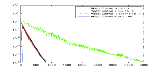
Figure 4.1: Residuals of adaptive Uzawa algorithm for Oseen problem with different preconditions ($32\times 32$ grids, $\nu=1$)

Figure 1 illustrated the residuals of Algorithm 3.1 for Oseen problem with different preconditioners. Obviously, the convergence of the residual curves confirms our analysis in Section 3, where we prove the convergence Theorem 3.1 for Algorithm 3.1.
From this figure, we can observe that, according to the number of iteration steps, the exact preconditioner $A_{s}$ is the most fast. While the preconditioners Cholinc and Ilu with tolerance of $10^{-1}$ take more iteration steps. The preconditioners Cholinc and Ilu almost need the same number of iterations, but the CPU time and flops in each step of Cholinc preconditioner are less than those of the preconditioner Ilu. The Jacobi preconditioner takes even more iteration steps, but it sometimes needs less CPU time, due to its simplicity, which can be seen from the test on N-S equation in the following. Moreover, we observed that, when the tolerance is between $[10^{-1},10^{-4}]$, the iteration numbers of Cholinc and Ilu preconditioners are decreasing with smaller tolerance. When the tolerance is less than or equal to $10^{-4}$, the iteration numbers of preconditioners Cholinc and Ilu are almost the same as the exact preconditioner $A_{s}$.

Next, we consider the Navier-Stokes problem. Solving the Navier-Stokes problem corresponds to solve an Oseen problem in every Picard iteration. Hence, the strategies designed for Oseen problem can be applied to Navier-Stokes problem as well. We compare the Algorithm 3.1 with the algorithm of Bramble-Pasciak-Vassilev (BPV) with $\delta=0.1$, $\tau=0.01$ in [5] and Gmres algorithm with no preconditioning. Table I, Table II, Table III illustrated the number of iterations and CPU times (seconds) of three cases with different preconditioners when $\nu=0.01,0.1,$ and $1$, respectively.

	$n$=16			$n$=32
Algorithms	iter	CPU		iter	CPU
AdaptiveUzawa+Ilu(1e-4)	14	4.26		16	57.76
AdaptiveUzawa+Cholinc(1e-4)	13	0.91		15	21.00
AdaptiveUzawa+Jacobi	12	1.81		12	73.50
AdaptiveUzawa+Exact	13	2.82		13	28.13
BPV+Ilu(1e-4)	12	54.07		12	343.40
BPV+Cholinc(1e-4)	12	6.99		12	84.83
BPV+Jacobi	12	21.39		12	773.68
Gmres	11	14.17		11	96.76

Table 4.1: Comparison of the computation time for N-S with $\nu=0.01$

	$n$=16			$n$=32
Algorithms	iter	CPU		iter	CPU
AdaptiveUzawa+Ilu(1e-4)	7	1.26		14	34.59
AdaptiveUzawa+Cholinc(1e-4)	7	0.33		14	14.96
AdaptiveUzawa+Jacobi	15	0.87		12	32.68
AdaptiveUzawa+Exact	7	0.64		14	18.74
BPV+Ilu(1e-4)	7	523.43		14	153.94
BPV+Cholinc(1e-4)	7	3.05		14	44.40
BPV+Jacobi	7	10.94		7	461.29
Gmres	6	2.16		11	16.09

Table 4.2: Comparison of the computation time for N-S with $\nu=0.1$

	$n$=16			$n$=32
Algorithms	iter	CPU		iter	CPU
AdaptiveUzawa+Ilu(1e-4)	20	2.13		27	63.09
AdaptiveUzawa+Cholinc(1e-4)	16	0.70		27	32.24
AdaptiveUzawa+Jacobi	192	5.39		418	382.53
AdaptiveUzawa+Exact	16	1.12		28	40.65
BPV+Ilu(1e-4)	5	15.96		233	292.91
BPV+Cholinc(1e-4)	5	2.00		233	216.41
BPV+Jacobi	5	10.71		5	462.76
Gmres	4	6.62		5	202.92

Table 4.3: Comparison of the computation time for N-S with $\nu=1$

From these tables, we can see that: (1) According to CPU time, the preconditioner Cholinc is almost the same time as the exact preconditioner, and both are better than Jacobi and Ilu preconditioners. (2) The convergence rate of our algorithm is faster than Bramble-Pasciak-Vassilev (BPV) algorithm in [5], and is comparable to Gmres algorithm. (3) In our algorithm, $\tau_{i}$ can be updated in each iteration, requiring no prior estimate on the spectrum of Schur complement, but the convergence of BPV algorithm depends on the spectrum of preconditioners.

The streamline of velocity and the contour of pressure using the algorithm in Section 3 are shown in figure 2, where we use the adaptive Uzawa algorithm with the preconditioner obtained by the incomplete Cholesky factorization with the tolerance of $10^{-1}$.

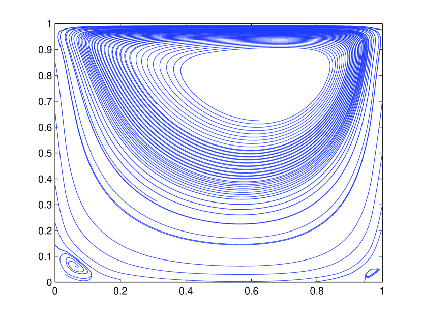
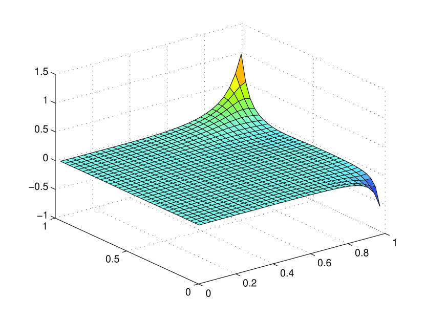
Figure 4.2: Streamline (left) and pressure contour (right) of Navier-Stokes problem ($32\times 32$ grids, $\nu=0.01$)

5 Conclusion

In this paper, we investigate an adaptive Uzawa algorithm with one variable relaxation parameter on generalized nonsymmetric saddle point problems. Our work is closely related to the work in [5] and [9]. In [9], Hu and Zou introduced the adaptive Uzawa algorithm with variable relaxation parameters for symmetric saddle point problems with $D=0$, while we extend this algorithm to the generalized nonsymmetric case. In [5], Bramble et al. discussed Uzawa algorithm on nonsymmetric saddle point problems with $D=0$ and proved its convergence under the assumption (1.5) and (1.6). We adopt their algorithm by adding a variable relaxation parameter and prove its convergence without the condition (1.5) and (1.6), that is to say, without any prior estimate on the spectrum of two preconditioned subsystems involved. Our numerical experiments on Oseen problem and N-S problem demonstrated the efficiency of our adaptive Uzawa algorithm. In fact, in our computation experiments, when we choose two variable relaxation parameters just like in [9], we also can get the convergence result. But its convergence theory is not completed yet. Moreover, the convergence result of nonlinear Uzawa type algorithm with variable relaxation parameters also still needs future work.

References

• [1] Z. Z. Bai, Z. Q. Wang, On parameterized inexact Uzawa methods for generalized saddle point problems, Numer. Linear Algebra Appl., 428(2008), pp. 2900-2932.
• [2] R. Bank, B. Welfert, H. Yserentant, A class of itertive methods for solving saddle point problems, Numer. Math., 56 (1990), pp. 645-666.
• [3] M. Benzi, G. H. Golub, J. Lisen, Numerical solution of saddle point problems, Acta Numerica (2005), pp. 1-137.
• [4] J. H. Bramble, J. E. Pasciak, A. T. Vassilev, Analysis of the inexact Uzawa algorithm for saddle point problem, SIAM J Numer. Anal., 34: 1072-1092, 1997.
• [5] J. H. Bramble, J. E. Pasciak, A. T. Vassilev, Uzawa type algorithms for nonsymmrtric saddle point problems, Math. Comp., 69 (1999), pp. 667-689.
• [6] Z. H. Cao, Fast Uzawa algorithm for generalized saddle point problems, Appl. Numer. Math., 46 (2003), pp. 157-171.
• [7] Z. H. Cao, Fast Uzawa algorithm for solving non-symmetric stabilized saddle point problems, Numer. Linear Algebra Appl., 11 (2004), pp. 1-24.
• [8] V. Girault, P. A. Raviart, Finite element approximation of the Navier-Stokes equations, Lecture Notes in Math., Springer-Verlag, New York, 1981.
• [9] Q. Hu, J. Zou, An iterative method with variable relaxation parameters for saddle point problems, SIAM J. Matrix Anal. Appl., 23 (2001), pp. 317-338.
• [10] Q. Hu, J. Zou, Two new variant of nonlinear inexact Uzawa algorithms for saddle-point problems, Numer. Math., 93 (2002), pp. 333-359.
• [11] Q. Hu, J. Zou, Nonlinear inexact Uzawa algorithms for linear and nonlinear saddle-point problems, SIAM J. Optim., 16 (2006), pp. 798-825.
• [12] K. Ito, H. Xiang, J. Zou, An inexact Uzawa algorithm for generalized saddle-point problems and its convergence, manuscript.
• [13] O. A. Karakashian, On a Galerkin-Lagrange multiplier method for the stationary Navier-Stokes equation, SIAM J. Numer. Anal., 19: 909-923, 1982.
• [14] P. Krzyzanowski, On block preconditioner for nonsymmetric saddle point problems, SIAM J. SCI. Comput., vol. 23, No. 1, pp. 157-169.
• [15] J. F. Lu, Z. Y. Zheng, A modified nonlinear inexact Uzawa algotithm with a variable relaxation parameter for the stabilized saddle point problem, SIAM J. Matrix Anal. Appl., 31 (2010), pp. 1934-1957.
• [16] R. Temam, Navier-Stokes Equations, North-Holland Publishing Co., New York, 1977.
• [17] Z. Tong, A. Sameh, On an iterative method for saddle point problems, Numer. Math., 79 (1998), pp. 643-646.
• [18] P. S. Vassilevski, Multilevel block factorization preconditioners: Matrix-based analysis and algorithms for solving finite element equations , Springer, 2008.
• [19] H. Xiang, L. Grigori, Kronecker product approximation preconditioners for convection-diffusion model problems, Numer. Linear Algebra Appl., (2010), pp. 691-712.