On the resolution of misspecified convex optimization and monotone variational inequality problems

Abstract

We consider a misspecified optimization problem that requires minimizing a function $f(x;\theta^{*})$ over a closed and convex set $X$ where $\theta^{*}$ is an unknown vector of parameters that may be learnt by a parallel learning process. In this context, we examine the development of coupled schemes that generate iterates $(x_{k},\theta_{k})$ as $k\to\infty$, then $x_{k}\to x^{*}$, a minimizer of $f(x;\theta^{*})$ over $X$ and $\theta_{k}\to\theta^{*}$. In the first part of the paper, we consider the solution of problems where $f$ is either smooth or nonsmooth. In smooth strongly convex regimes, we demonstrate that such schemes lead to a quantifiable degradation of the standard linear convergence rate. When strong convexity assumptions are weakened, it can be shown that the convergence in function values sees a modification in the convergence rate of ${\cal O}(1/K)$ by an additive factor $\|\theta_{0}-\theta^{*}\|{\cal O}(q_{g}^{K}+1/K)$ where $\|\theta_{0}-\theta^{*}\|$ represents the initial misspecification in $\theta^{*}$ and $q_{g}$ denotes the contractive factor associated with the learning process. In both convex and strongly convex regimes, diminishing steplength schemes are also provided and are less reliant on the knowledge of problem parameters. Finally, we present an averaging-based subgradient scheme and show that the optimal constant steplength leads to a modification in the rate by $\|\theta_{0}-\theta^{*}\|{\cal O}(q_{g}^{K}+1/K)$, implying no effect on the standard rate of ${\cal O}(1/\sqrt{K})$. In the second part of the paper, we consider the solution of misspecified monotone variational inequality problems, motivated by the need to contend with more general equilibrium problems as well as the possibility of misspecification in the constraints. In this context, we first present a constant steplength misspecified extragradient scheme and prove its asymptotic convergence. This scheme is reliant on problem parameters (such as Lipschitz constants) and leads us to present a misspecified variant of iterative Tikhonov regularization. Numerics support the asymptotic and rate statements with one important observation: it appears that the rate bound derived for strongly convex problems appears to be slack in that the standard linear rate is again observed, despite the theoretical prediction that learning leads to degradation.

1 Introduction

Traditionally, the field of deterministic optimization has focused on the problem of minimizing a function $f(x)$ over a prescribed set $X$ and it is generally assumed that the decision maker has complete knowledge of both the function $f$ and the set $X$ (cf. [1, 2]). In many settings, problem data may be uncertain, severely limiting the applicability of deterministic methods. Initiated through the research by Dantzig [3] and Beale [4], stochastic programming has represented a popular avenue for addressing risk-neutral as well as risk-averse static and adaptive (recourse-based) decision-making problems [5, 6] in developing both static as well as adaptive (recourse-based) models. An alternative approach has found merit by obviating the need for distributional information and instead focuses on obtaining solutions that are robust to parametric uncertainty over a prescribed (uncertainty) set [7, 8]. In either instance, a subset of parameters is natively uncertain. Our focus is on a class of problems in which the vector parameters is $\theta^{*}$, a fixed but unknown vector, that may be learnt through a related but distinct learning process. We provide a clearer understanding of our problem of interest by considering a motivating problem.

Data-driven stochastic optimization: Standard models for stochastic optimization have required the solution of the following problem [5, 6]:

$$\min_{x\in X}\,\mathbb{E}_{\theta^{*}}[f(x;\xi(\omega))], (\theta^{*})$$ (StochOpt)

where $X\subseteq\mathbb{R}^{n}$, $f:X\times\mathbb{R}^{d}\to\mathbb{R}$, $\xi:\Omega\to\mathbb{R}^{d}$ is a $d-$dimensional random variable, and $(\Omega,{\mathcal{F}},\mathbb{P}_{\theta^{*}})$ denotes the probability space. Note that $\theta^{*}$ represents the parameters of the distribution $\mathbb{P}$. Unfortunately, a key shortcoming in the use of standard models necessitates knowledge of $\theta^{*}$, often a stringent requirement. Instead, suppose $\theta^{*}$ may be learnt by a suitably defined maximum likelihood estimation (MLE) problem [9], captured by a metric $g(\theta)$, and formally defined as follows:

$$\min_{\theta\in\Theta}\,g(\theta).$$ (MLE)

Generally, in most practically occurring problems, the MLE problem is often massive and one avenue lies in generating sequences $\{(x_{k},\theta_{k})\}$ such that $x_{k}$ is an approximate solution of (StochOpt$(\theta_{k})$).

A range of other problems can be cast in a similar regime. For instance, in traffic equilibrium problems [10], a common assumption is that the demand pattern and the travel times are known vectors, assumptions that are often hard to justify in practice. Similarly, in a range of production planning problems, it is routinely assumed that cost and demand information is accurately available when in fact, it needs to be empirically estimated. Consequently, one approach lies in conducting such an estimation through a parallel learning process. Yet another problem that can be cast under this umbrella is the well studied multi-armed bandit problem [11]. In such a problem, a gambler is faced with a choosing from a collection of slot machines at every step without a prior knowledge of the average reward distribution. If one could view the learning problem associated with the reward distributions as a parallel estimation problem, this may be one avenue towards developing algorithmic techniques. Motivated by this new set of decision-making problems, we consider the static misspecified convex optimization problem $(\cal C(\theta^{*}))$, defined as follows:

$$\min_{x\in X}\,f(x,\theta^{*}), \cal C(\theta^{*})$$ ()

where $x\in\mathbb{R}^{n}$, $f:X\times\Theta\to\mathbb{R}$ is a convex function in $x$ for every $\theta\in\Theta\subseteq\mathbb{R}^{m}$. Suppose $\theta^{*}$ denotes the solution to a convex learning problem denoted by $(\cal L)$:

$$\min_{\theta\in\Theta}\ g(\theta), {\cal L}$$ ()

where $g:\mathbb{R}^{m}\to\mathbb{R}$ is a convex function in $\theta$ and is defined on a closed and convex set $\Theta.$ Consequently, we consider gradient methods in which sequences $\{x_{k}\}$ and $\{\theta_{k}\}$ may be generated with the goal that

$$\lim_{k\to\infty}x_{k}=x^{*}\in X^{*}\mbox{ and }\lim_{k\to\infty}\theta_{k}=\theta^{*},\mbox{ where }X^{*}\triangleq\displaystyle{\mathop{\rm argmin}_{x\in X}f(x;\theta^{*})}.$$

It should be noted that the second author has examined the counterpart of such problems in stochastic regimes where stochastic approximation schemes are employed [12].

1.1 Alternate and related avenues

Given that the focus lies on solving $({\cal C}(\theta^{*}))$ and $(\cal L)$ simultaneously, at least three approaches assume relevance and are described next.

A sequential approach:

A natural question is whether this problem could indeed be solved in a sequential fashion. For instance, one approach could be to compute $\theta^{*}$ in the first stage and subsequently solve ($\cal C(\theta^{*})$). Yet such an avenue is complicated by several challenges: (i) First, the problem ($\cal L$) is often of a large or massive scale and accurate/exact solutions of this problem are needed in finite time to utilize this approach. However, the claim that finite termination schemes are available is a strong one. In fact, even in the rare instance when this requirement is met, the number of steps might be far too large in practice. Consequently, such an approach leads to obtaining an approximation of $\theta^{*}$, given by a vector $\hat{\theta}$ and cannot provide asymptotically accurate solutions. (ii) Second, if the process is terminated prior to the commencing with the computation of $x^{*}$, then the resulting computational effort would be wasted in that we have no guarantees regarding the solution. We consider precisely such an approach in the context of economic dispatch problems, discussed in Section 4. Table  1 shows the importance of terminating the learning problem after a sufficiently large number of iterations via a sequential approach. In particular, for smaller problems with $5$ generators, $15,000$ learning steps suffice in getting reasonably accurate estimates of $x^{*}$ while the same number of iterations prove insufficient for getting accurate solutions for networks with $20$ generators. In contrast, our focus lies in developing techniques that can provide asymptotically accurate solutions equipped with global non-asymptotic error bounds.

Learning steps	Computational steps	number of generators $=$ 5		number of generator$=$ 40
		$\|\theta_{k}-\theta^{*}\|$	$\frac{\|f(x_{k},\theta^{*})-f^{*}\|}{1+f^{*}}$	$\|\theta_{k}-\theta^{*}\|$	$\frac{\|f(x_{k},\theta^{*})-f^{*}\|}{1+f^{*}}$
1000	15000	$6.43$e$0$	$6.49$e-$2$	$2.10$e$1$	$2.33$e-$1$
5000	15000	$3.34$e$0$	$4.25$e-$2$	$1.95$e$1$	$9.05$e-$2$
10000	15000	$1.48$e-$1$	$8.80$e-$3$	$1.77$e$1$	$8.08$e-$2$
15000	15000	$1.63$e-$2$	$4.00$e-$4$	$1.06$e$1$	$6.60$e-$2$

Table 1: Sequential approach: Effect of problem size on accuracy

A variational approach:

Given that a sequential approach may not always be satisfactory, a partial resolution lies in considering a variational approach where the overall problem is cast as a static variational inequality problem [10]. If $X\subseteq\mathbb{R}^{n}$ and $F:\mathbb{R}^{n}\to\mathbb{R}^{n}$, then it may be recalled that VI$(X,F)$ requires an $x\in X$ such that $(y-x)^{T}F(x)\,\geq\,0$ for all $\ y\ \in\ X.$ Under convexity assumptions, it can be shown with relative ease that $(x^{*},\theta^{*})\triangleq z^{*}$ is a solution of VI$(Z,H)$ if $Z\triangleq X\times\Theta$ and $H(z)=(\nabla_{x}f(x,\theta);\nabla_{\theta}g(\theta)).$ But the solution of VI$(Z,H)$ via projection-based techniques [13] remains a challenge since $H(z)$ is generally not a monotone map over the set $Z$ even if $f$ and $g$ are convex $C^{1}$ functions in $x$ and $\theta$, respectively; it may be recalled that a map $H$ is monotone over $Z$ if for every $z_{1},z_{2}\in Z$, $(H(z_{1})-H(z_{2}))^{T}(z_{1}-z_{2})\geq 0$. But there are no available first-order schemes for computing solutions to non-monotone variational inequality problems, severely limiting the utility of such an approach. Yet, despite the inherently challenging nature of the joint variational problem, our goal remains in deriving non-asymptotic rates of convergence for gradient methods for such problems by leveraging the structure of the problem and ascertaining the impact that learning has on the rates.

A robust optimization approach:

Robust optimization, a subfield of optimization, considers obtaining solutions that are robust to parametric uncertainty [8, 14, 7]. In such problems, rather than a vector $\theta^{*}$, a part of the problem input is the uncertainty set, say ${\cal U}_{\theta}$. In such a case, the relevant robust optimizaton problem attempts to obtain an $x$ that minimizes the worst-case value that $f(x,\theta)$ takes over ${\cal U}_{\theta}$:

$$\min_{x\in X}\,\max_{\theta\in{\cal U}_{\theta}}f(x,\theta).$$

In contrast, our framework is fundamentally different in that the vector $\theta^{*}$ is a deterministic and unknown vector that can be learnt. To provide a clearer comparison, the learning scheme solves the following problem

$$\min_{x\in X}\,f(x;\theta^{*})\quad\mbox{where}\quad\theta^{*}=\mathop{\rm argmin}_{\theta\in\Theta}g(\theta).$$

Learning while doing schemes:

Finally, we note the surge of interest in algorithms which incorporate learning directly into the optimization phase. Early instances of such problems were seen in the form of the multi-armed bandit problem [15, 11] in which a decision-maker simultanelusly acquires new knowledge and leverages existing knowledge in optimizing decisions. In contrast with the current context, the learning problem is no longer static and available a priori; instead, it evolves in time as a consequence of aggregating observations. In response to such challenges, Agarwal et al. have developed techniques in the context on online linear programming [16] as well as stylized counterparts in the context of revenue management [17, 18]. A rather different tack is taken in the work by Jiang et al. [19], where the problem ${\cal L}$ is replaced by a sequence of learning problems ${\cal L}_{1},\ldots,{\cal L}_{k}$, such that the index of $k$ represents the number of data points used within the construction of the associated estimation (regression) problem. The solution of the $k$th learning problem is denoted by $\theta_{k}$ and under suitable assumptions, $\{\theta_{k}\}\to\theta^{*}$, where $\theta^{*}$ is a solution to the limiting problem. If $\theta_{k}$ is used within the scheme for computing $x$, then probabilistic convergence statements are provided for $\{x_{k}\}$ in the context of distributed projection-based schemes for stochastic Nash games, leading to monotone variational inequality problems. We note that offline schemes provide a benchmark in terms of ascertaining the cost of obtaining observations over time, rather than a priori, allowing us to derive metrics to relate online schemes with their offline counterparts (such as through competitive ratios for instance).

1.2 Contributions and outline

In this paper, we investigate the global convergence and rate analysis of joint first-order gradient methods under a variety of convexity, Lipschitzian, and boundedness requirements. Suppose $\gamma_{f,k}$ and $\gamma_{g,k}$ denote steplength for optimization and learning at iteration $k$. If $\Pi_{Y}(y)$ denotes the Euclidean projection of a vector $y$ on the set $Y$, then consider the following prototypical update:

Algorithm 1 (Joint gradient scheme).

Given $x_{0}\in X$ and $\theta_{0}\in\Theta$ and sequences ${\gamma_{f,k},\gamma_{g,k}}$,

$$x_{k+1} :=\Pi_{X}\left(x_{k}-\gamma_{f,k}\nabla_{x}f(x_{k},\theta_{k})\right),\quad \forall k\ \geq\ 0, (\theta_{k})$$ (Opt)

$$\theta_{k+1} :=\Pi_{\Theta}\left(\theta_{k}-\gamma_{g,k}\nabla_{\theta}g(\theta_{k})\right),\ \quad\quad \forall k\ \geq\ 0.$$ (Learn)

In our proposed scheme, we take a gradient step in the $x$-space using an estimate $\theta_{k}$ of $\theta^{*}$ and a simultaneous step in the $\theta-$space. Note that instead of using the exact gradient $\nabla_{x}f(x_{k},\theta^{*})$ at the $k$th iterate, we employ $\nabla_{x}f(x_{k},\theta_{k})$ as the gradient estimate and $r_{k}=\nabla_{x}f(x_{k},\theta_{k})-\nabla_{x}f(x_{k},\theta^{*})$ represents the error in the gradient at iteration $k$. Recent literature on inexact gradient schemes has investigated convergence properties and rate analysis for various schemes using inexact gradients with bounded error [20, 21, 22, 23, 24]. Our framework is distinct in that we develop a broader framework of gradient, extragradient, and regularized schemes for solving both optimization and variational inequality problems through the provision of modified algorithmic requirements (such as those on steplengths), asymptotics, and enhanced rate statements. The framework is developed under the caveat that the inexactness (in gradient estimates) decays to zero at a prescribed rate, a consequence of obtaining increasing accurate estimates of $\theta_{k}$ when taking the gradient step in the $x-$space. The main contributions of this work can be captured as follows:

(i) Convex optimization: In the first part of this paper, we develop asymptotics and rate statements for misspecified convex optimization problems in smooth and nonsmooth settings and assume that the learning problem is strongly convex, unless mentioned otherwise: (a) Smooth optimization problems: Our first set of results in the smooth regime demonstrate that constant steplength schemes are convergent but lead to a quantifiable decay in the linear convergence rate characteristic of constant steplength gradient methods. Unfortunately, such techniques are heavily reliant on the knowledge of certain problem parameters, in the absence of which we show that diminishing steplength sequences are also convergent. When the strong convexity assumptions are weakened, we note that the presence of learning leads to modification of the convergence rate in function values by an additive factor given by $\|\theta_{0}-\theta^{*}\|{\cal O}\left(q_{g}^{K}+{1/K}\right)$ where $\theta_{0}$ represents our initial estimate of $\theta^{*}$, $q_{g}$ denotes the contractive constant in the learning problem. Finally, we demonstrate that when the learning problem loses strong convexity, under a suitably defined weak-sharpness requirement, global convergence can still be retained; (b) Nonsmooth optimization problems: When the optimization problem is nonsmooth, it can be shown that while the overall convergence rate of the proposed misspecified subgradient methods is still ${\cal O}({1/\sqrt{K}})$, a similar additive factor emerges of the form $\|\theta_{0}-\theta^{*}\|{\cal O}\left(q_{g}^{K}+{1/K}\right).$ A summary of the rate statements is provided in Table 2.

	Computation	Computation & Learning
Strongly convex/diff.	Linear	Sublinear
convex/diff.	${\cal O}(1/K)$	${\cal O}(1/K)+\|\theta_{0}-\theta^{*}\|{\cal O}(1/K+q_{g}^{K})$
convex/nonsmooth.	${\cal O}(1/\sqrt{K})$	${\cal O}(1/\sqrt{K})+\|\theta_{0}-\theta^{*}\|{\cal O}(1/K+q_{g}^{K})$

Table 2: Summary of rate statements

(ii) Monotone variational inequality problems: Variational inequality problems represent a broad framework for capturing optimization and equilibrium problems and assume particular relevance, given that misspecification may arise in the constraints. In the second part of this paper, we consider two sets of schemes for resolving misspecified variational inequality problems. Of these, the first avenue is a constant steplenth misspecified extragradient scheme for monotone variational inequality problems. However, this approach requires an accurate estimate of suitable Lipschitz parameters. Consequently, we present a misspecified variant of the iterative Tikhonov regularization framework to misspecified monotone regimes.

(iii) Numerics: We develop a set of test problems based on economic dispatch problems [25] with misspecified cost and demand. The numerics support the asymptotic statements and the validity of the bounds.

2 Misspecified Convex Optimization

In this section, we will consider two settings differentiated by the assumptions on the function $f(x,\theta)$ in $(\cal C(\theta^{*}))$ and the function $g(\theta)$ in $(\cal L)$. In Section 2.1, we examine gradient-based methods where $f(x,\theta)$ is differentiable in $x$ for every $\theta$ while in Section 2.2, we weaken the smoothness requirement on $f(x,\theta)$. In each setting, we provide both constant steplength schemes with associated complexity statements as well as diminishing steplength schemes that are less reliant on problem parameters.

2.1 Smooth convex optimization

In this section, we consider regimes where both the optimization and learning problems are differentiable and distinguish the cases based on the convexity assumptions on the problem. Specifically, in subsection  2.1.1, we provide convergence statements and rate analysis when both problems are strongly convex. Next, in subsection  2.1.2, we weaken the strong convexity assumption on the computational problem to mere convexity and provide rate statements in such settings. Finally, in subsection  2.1.3, we relax the strongly convex assumption of the learning function and analyse the case when the solution set of the learning problem satisfies a weak sharpness assumption. We now list several key assumptions used during our analysis. We begin with a differentiability assumption on $f$ and $g$.

Assumption 1.

The function $f(x,\theta)$ is continuously differentiable in $x$ for all $\theta\in\Theta$ and function $g$ is continuously differentiable in $\theta$.

Next, we impose a Lipschitzian assumption on $f$ in $x$, uniformly in $\theta$.

Assumption 2.

The gradient map $\nabla_{x}f(x;\theta)$ is Lipschitz continuous in $x$ with constant $G_{f,x}$ uniformly over $\theta\in\Theta$ or

$$\|\nabla_{x}f(x_{1},\theta)-\nabla_{x}f(x_{2},\theta)\|\leq G_{f,x}\|x_{1}-x_{2}\|,\qquad\forall x_{1},x_{2}\in X,\quad\forall\theta\in\Theta.$$

Additionally, the gradient map $\nabla_{\theta}g$ is Lipschitz continuous in $\theta$ with constant $G_{g}$.

Finally, we impose a requirement on steplength sequences for the computational and learning problems required in the diminishing steplength regime.

Assumption 3.

Let $\{\gamma_{f,k}\}$ and $\{\gamma_{g,k}\}$ be diminishing nonnegative sequences chosen such that $\sum_{k=1}^{\infty}\gamma_{f,k}=\infty$, $\sum_{k=1}^{\infty}\gamma_{f,k}^{2}<\infty$, $\sum_{k=1}^{\infty}\gamma_{g,k}=\infty$, and $\sum\limits_{k=1}^{\infty}\gamma_{g,k}^{2}<\infty$.

2.1.1 Strongly convex optimization and learning

In this subsection, convergence statements for the iterates produced by Algorithm 1 are provided under the following strong convexity assumption.

Assumption 4.

The function $f$ is strongly convex in $x$ with constant $\eta_{f}$ for all $\theta\in\Theta$ and the function $g$ is strongly convex with constant $\eta_{g}$.

We impose an additional Lipschitzian assumption on $\nabla_{x}f(x^{*};\theta)$ in $\theta$.

Assumption 5.

The gradient $\nabla_{x}f(x^{*},\theta)$ is Lipschitz continuous in $\theta$ with constant $L_{\theta}$.

Before providing the main results, we introduce the following Lemma from [26]:

Lemma 1.

Let the following hold:

$$u_{k+1}\leq q_{k}u_{k}+\alpha_{k},\quad 0\leq q_{k}<1,\quad\alpha_{k}\geq 0,\quad\sum_{k=1}^{\infty}(1-q_{k})=\infty,\quad\lim_{k\to\infty}\frac{\alpha_{k}}{(1-q_{k})}=0.$$

Then, $\lim_{k\to\infty}u_{k}\leq 0$. In particular, if $u_{k}\geq 0$, then $u_{k}\to 0$.

Our first result provides a convergence statement under a constant steplength assumption.

Proposition 2 (Constant step length scheme).

Let Assumptions 1 2, 4 and  5 hold and $\gamma_{f,k}$ and $\gamma_{g,k}$ are fixed at $\gamma_{f}$ and $\gamma_{g}$, respectively so that $0<\gamma_{f}<{2/G_{f,x}}$ and $0<\gamma_{g}<2/G_{g}$. Then, the sequence $\{x_{k},\theta_{k}\}$ generated by Algorithm 1 converges to $x^{*}\in X$ and $\theta^{*}\in\Theta$, respectively.

Proof.

By nonexpansivity of the Euclidean projector and triangle inequality, $\|x_{k+1}-x^{*}\|$ can be bounded as follows:

$$\quad\,\|x_{k+1}-x^{*}\|$$

$$=\|\Pi_{X}(x_{k}-\gamma_{f}\nabla_{x}f(x_{k},\theta_{k}))-\Pi_{X}(x^{*}-\gamma_{f}\nabla_{x}f(x^{*},\theta^{*}))\|$$

$$\leq\|(x_{k}-x^{*})-\gamma_{f}(\nabla_{x}f(x_{k},\theta_{k})-\nabla_{x}f(x^{*},\theta^{*}))\|$$

$$\leq\|(x_{k}-x^{*})-\gamma_{f}(\nabla_{x}f(x_{k},\theta_{k})-\nabla_{x}f(x^{*},\theta_{k})\|+\gamma_{f}\|\nabla_{x}f(x^{*},\theta_{k})-\nabla_{x}f(x^{*},\theta^{*}))\|.$$ (1)

The first term in (1) can be further bounded by first writing the following expansion:

$$\|(x_{k}-x^{*})-\gamma_{f}(\nabla_{x}f(x_{k},\theta_{k})-\nabla_{x}f(x^{*},\theta_{k}))\|^{2} =\|x_{k}-x^{*}\|^{2}+\gamma_{f}^{2}\|\nabla_{x}f(x_{k},\theta_{k})-\nabla_{x}f(x^{*},\theta_{k})\|^{2}$$

$$-2\gamma_{f}(x_{k}-x^{*})^{T}(\nabla_{x}f(x_{k},\theta_{k})-\nabla_{x}f(x^{*},\theta_{k})).$$ (2)

Under the assumption of Lipschitz continuity of $\nabla_{x}f(x,\theta)$ in $x$, it follows that

$$\|\nabla_{x}f(x_{k},\theta_{k})-\nabla_{x}f(x^{*},\theta_{k})\|^{2}\leq G_{f,x}(x_{k}-x^{*})^{T}(\nabla_{x}f(x_{k},\theta_{k})-\nabla_{x}f(x^{*},\theta_{k})).$$

By combining the above inequality with (2), we obtain

$$\quad\|(x_{k}-x^{*})-\gamma_{f}(\nabla_{x}f(x_{k},\theta_{k})-\nabla_{x}f(x^{*},\theta_{k}))\|^{2}$$

$$\leq\|x_{k}-x^{*}\|^{2}-\gamma_{f}(2-\gamma_{f}G_{f,x})(x_{k}-x^{*})^{T}(\nabla_{x}f(x_{k},\theta_{k})-\nabla_{x}f(x^{*},\theta_{k})).$$ (3)

In addition, under strong convexity of $f(x;\theta)$ in $x$, it follows that

$$(x_{k}-x^{*})^{T}(\nabla_{x}f(x_{k},\theta_{k})-\nabla_{x}f(x^{*},\theta_{k}))\geq\eta_{f}\|x_{k}-x^{*}\|^{2}.$$

Thus, inequality (3) becomes

$$\|(x_{k}-x^{*})-\gamma_{f}(\nabla_{x}f(x_{k},\theta_{k})-\nabla_{x}f(x^{*},\theta_{k}))\|^{2} \leq\|x_{k}-x^{*}\|^{2}-\gamma_{f}\eta_{f}(2-\gamma_{f}G_{f,x})\|x_{k}-x^{*}\|^{2}$$

$$=\big{(}1-\gamma_{f}\eta_{f}(2-\gamma_{f}G_{f,x})\big{)}\|x_{k}-x^{*}\|^{2}.$$ (4)

Note that since $\gamma_{f}<({2/G_{f,x}})$, then it follows that $\big{(}1-\gamma_{f}\eta_{f}(2-\gamma_{f}G_{f,x})\big{)}<1.$ The second term in $\eqref{con_expan1}$ is bounded by leveraging the Lipschitz continuity of $\nabla_{x}f(x^{*},\theta)$ in $\theta$:

$$\|\gamma_{f}(\nabla_{x}f(x^{*},\theta_{k})-\nabla_{x}f(x^{*},\theta^{*}))\|\leq\gamma_{f}L_{\theta}\|\theta_{k}-\theta^{*}\|.$$ (5)

Now by combining (1), (4), and (5), we obtain the following bound:

$$\|x_{k+1}-x^{*}\| \leq q_{x}\|x_{k}-x^{*}\|+q_{\theta}\|\theta_{k}-\theta^{*}\|,$$ (6)

where $q_{x}\triangleq\sqrt{\big{(}1-\gamma_{f}\eta_{f}(2-\gamma_{f}G_{f,x})\big{)}}$ and $q_{\theta}\triangleq\gamma_{f}L_{\theta}$. To show that $\|x_{k}-x^{*}\|\to 0$ as $k\to\infty$, we may employ Lemma 1. This requires showing the following:

$${(i)}\quad\sum_{k=1}^{\infty}(1-q_{x})=\infty;\qquad{(ii)}\quad\lim_{k\to\infty}\frac{q_{f,\theta}\|\theta_{k}-\theta^{*}\|}{1-q_{x}}=0.$$

Since $q_{x}<1$, $(i)$ is satisfied. In addition, by the Lipschitz continuity of $\nabla_{\theta}g$ and choosing $\gamma_{g}$ such that $0<\gamma_{g}<2/G_{g}$, $\|\theta_{k}-\theta^{*}\|\to 0$ as $k\to\infty$. Consequently, condition $(ii)$ is met as well, completing the proof. ∎

In many instances, while we may be able to claim strong convexity or Lipschitz continuity, the precise bounds may be unavailable. However, an incorrect choice of a steplength may lead to divergence, motivating the need for an alternate approach. To this end, we employ a diminishing steplength sequence that does not necessitate the knowledge of either the convexity constant or the Lipschitz constant. We outline the proof of convergence in the next Proposition.

Proposition 3 (Diminishing steplength schemes).

Let Assumptions 1, 2, 4, and  5 hold. Additionally, let $\gamma_{f,k}$ be defined based on Assumption  3 and $\gamma_{g,k}$ be fixed at $\gamma_{g}$ so that $0<\gamma_{g}<2/G_{g}$.Then, the sequence $\{x_{k},\theta_{k}\}$ generated by Algorithm 1 converges to $x^{*}\in X$ and $\theta^{*}\in\Theta$, respectively.

Proof.

We use a similar line of argument as in Proposition 2 to obtain the following bound:

$$\|x_{k+1}-x^{*}\|\leq q_{x,k}\|x_{k}-x^{*}\|+q_{\theta,k}\|\theta_{k}-\theta^{*}\|,$$ (7)

where for sufficiently large $k$, we have that $q_{x,k}\triangleq{(1-\gamma_{f,k}\eta_{f}(2-\gamma_{f,k}G_{f,x}))^{1/2}}<1$ and $q_{\theta,k}\triangleq\gamma_{f,k}L_{\theta}$. By Assumption 3, we have that $\sum_{k=1}^{\infty}(1-q_{x,k})=\infty$. Furthermore, we have the following simplification of condition (ii) of Lemma 1:

$$\lim_{k\to\infty}\frac{\gamma_{f,k}L_{\theta}\|\theta_{k}-\theta^{*}\|}{(1-q_{x,k})} =\lim_{k\to\infty}\frac{(1+q_{x,k})L_{\theta}\|\theta_{k}-\theta^{*}\|}{{\eta_{f}(2-\gamma_{f,k}G_{f,x})}}=0$$

since $q_{x,k}\to 0$ and $\gamma_{f,k}\to 0$ and $\|\theta_{k}-\theta^{*}\|\to 0$ as $k\to\infty$. Therefore, the conditions of Lemma 1 are satisfied and $\|x_{k}-x^{*}\|\to 0$ as $k\to\infty$. ∎

It is well known that under strong convexity assumption, the iterates generated from the projected gradient method converge at a geometric rate [27]. However, when learning is incorporated, it is expected that this rate drops. Next, we analyze the impact introduced by learning.

Proposition 4 (Rate analysis in strongly convex regimes).

Let Assumptions 1, 2, 4 and  5 hold. In addition, assume that $\gamma_{f}$ and $\gamma_{g}$ are chosen such that $0<\gamma_{f}<2/G_{f,x}$ and $0<\gamma_{g}{<}{2/G_{g}}$. Let $\{x_{k},\theta_{k}\}$ be the sequence generated by Algorithm 1. Then for every $k\geq 0$, we have the following:

$$\|x_{k+1}-x^{*}\| \leq q_{x}^{k+1}\|x_{0}-x^{*}\|+(k+1)q_{\theta}q^{k}\|\theta_{0}-\theta^{*}\|,$$

where $q_{x}\triangleq(1-\gamma_{f}\eta_{f}(2-\gamma_{f}G_{f,x}))^{1/2}$, $q_{\theta}\triangleq\gamma_{f}L_{\theta}$, $q_{g}\triangleq(1-\gamma_{g}\eta_{g}(2-\gamma_{g}G_{g}))^{1/2}$, and $q\triangleq\max(q_{x},g_{g})$.

Proof.

Under the assumption of strong convexity of $g$, the learning algorithm has a globally geometric rate of convergence when employing constant stepsize $\gamma_{g}$ where $0<\gamma_{g}<2/G_{g}$; specifically,

$$\|\theta_{k+1}-\theta^{*}\|\leq q_{g}^{k+1}\|\theta_{0}-\theta^{*}\|,\quad\forall k\ \geq\ 0.$$ (8)

where $q_{g}\triangleq(1-\gamma_{g}\eta_{g}(2-\gamma_{g}G_{g}))^{1/2}<1$ since $\gamma_{g}<2/G_{g}$ . To obtain the convergence rate for the joint scheme, we expand $\eqref{bnd_csl}$ to obtain the following bound:

$$\|x_{k+1}-x^{*}\| \leq q_{x}^{k+1}\|x_{0}-x^{*}\|+q_{\theta}\sum_{i=0}^{k}q_{x}^{i}\|\theta_{k-i}-\theta^{*}\|\qquad\forall\ k\geq 0.$$ (9)

We may further expand $\eqref{bnd_expn}$ using $\eqref{geom_cr}$ to simplify the bound as below:

$$\|x_{k+1}-x^{*}\| \leq q_{x}^{k+1}\|x_{0}-x^{*}\|+q_{\theta}\sum_{i=0}^{k}q_{x}^{i}q_{g}^{k-i}\|\theta_{0}-\theta^{*}\|\leq q_{x}^{k+1}\|x_{0}-x^{*}\|+\underbrace{(k+1)q_{\theta}q^{k}\|\theta_{0}-\theta^{*}\|,}_{\tiny\mbox{Degradation from learning}}$$

where $q\triangleq\max(q_{x},q_{g})$. Note that condition $\gamma_{f}<2/G_{f,x}$ guarantees that $q_{x}<1$, implying that $q=\max(q_{x},q_{g})$ is less than 1. ∎

Remark: Notably, the presence of learning leads to a degradation in the convergence rate from the standard linear rate to a sub-linear rate. Furthermore, it is easily seen that when we have access to the true $\theta^{*}$, the original rate may be recovered.

2.1.2 Convex optimization with strongly convex learning

In this subsection, we weaken the rather stringent assumptions of strong convexity of $f(x,\theta)$ in $x$ for every $\theta\in\Theta$.

Assumption 4b. The function $f$ is convex in $x$ for all $\theta\in\Theta$ and the function $g$ is strongly convex with constant $\eta_{g}$.

In addition, we make the following assumptions:

Assumption 6.

1. The sets $X$ and $\Theta$ are compact and $\sup_{x\in X}\|x\|\leq C$, where $C$ is a constant.

2. The gradient map $\nabla_{x}f(x;\theta)$ is uniformly Lipschitz continuous in $\theta$ with constant $G_{f,\theta}$:

   $$\|\nabla_{x}f(x,\theta_{1})-\nabla_{x}f(x,\theta_{2})\|\leq G_{f,\theta}\|\theta_{1}-\theta_{2}\|,\quad\forall\theta_{1},\theta_{2}\in\Theta,x\in X.$$

Assumption 7.

There exists a constant $L_{f,\theta}$ such that $|f(x,\theta_{1})-f(x,\theta_{2})|\leq L_{f,\theta}\|\theta_{1}-\theta_{2}\|,\quad\forall\theta_{1},\theta_{2}\in\Theta,x\in X.$

Before presenting the main result, we introduce the following Lemma from [28].

Lemma 5.

Let $\beta_{k},\upsilon_{k},\alpha_{k}\geq 0$ for all $k$. Furthermore, suppose the following holds for all $k$:

$$u_{k+1}\leq(1+\beta_{k})u_{k}-\upsilon_{k}+\alpha_{k}.$$

Suppose $\sum_{k}\alpha_{k}<\infty$ and $\sum_{k}\beta_{k}<\infty$. Then $\lim_{k\to\infty}u_{k}=\bar{u}\geq 0$ and $\sum_{k}\upsilon_{k}<\infty$.

In the following proposition, we prove the convergence of the iterates generated by Algorithm  1 under the convexity requirements on $f(x;\theta)$. We also provide the rate statement.

Proposition 6 (Constant steplength scheme with averaging).

Let Assumptions  1, 2, 4b, 6 and  7 hold and stepsizes $\gamma_{f,k}$ and $\gamma_{g,k}$ be fixed at constants $\gamma_{f}$ and $\gamma_{g}$ so that $0<\gamma_{g}<2/G_{g}$ and $0<\gamma_{f}\leq 1/G_{f,x}$. Let the sequence $\{x_{k},\theta_{k}\}$ be generated by Algorithm  1 and suppose $\bar{x}_{k}$ is defined as

$$\bar{x}_{k}\triangleq\frac{\displaystyle\sum_{i=0}^{k-1}x_{i+1}}{k}.$$

Then the following hold:

1. In addition, if $a_{x}=\frac{\|x_{0}-x^{*}\|^{2}}{2\gamma_{f}}$ and $b_{\theta}\triangleq\frac{CG_{f,\theta}}{1-q_{g}},$ then the following holds:

   $$\left|f\left(\bar{x}_{K},\theta_{K}\right)-f(x^{*},\theta^{*})\right|\leq\frac{a_{x}}{K}+\|\theta_{0}-\theta^{*}\|\left(\frac{b_{\theta}}{K}+L_{f,\theta}q_{g}^{K}\right).$$

2. ${\displaystyle\lim_{k\to\infty}}f\left(\bar{x}_{k},\theta_{k}\right)=f(x^{*},\theta^{*}).$

Proof.

(i)  Recall the following by the mean-value theorem, the Cauchy-Schwartz inequality, and Lipschitz continuity of the gradient map $\nabla_{x}f(x,\theta^{*})$ in $x$:

$$f(y,\theta^{*}) =f(x,\theta^{*})+\nabla_{x}f(x,\theta^{*})^{T}(y-x)+\int_{0}^{1}(\nabla_{x}f(x+t(y-x),\theta^{*})-\nabla_{x}f(x,\theta^{*}))(y-x)dt$$

$$\leq f(x,\theta^{*})+\nabla_{x}f(x,\theta^{*})^{T}(y-x)+\int_{0}^{1}\|(\nabla_{x}f(x+t(y-x),\theta^{*})-\nabla_{x}f(x,\theta^{*}))\|\|(y-x)\|dt$$

$$\leq f(x,\theta^{*})+\nabla_{x}f(x,\theta^{*})^{T}(y-x)+\int_{0}^{1}G_{f,x}t\|y-x\|\|(y-x)\|dt$$

$$=f(x,\theta^{*})+\nabla_{x}f(x,\theta^{*})^{T}(y-x)+{1\over 2}G_{f,x}\|y-x\|^{2}.$$

If we set $y=x_{i+1}$ and $x=x_{i}$ and since $G_{f,x}\leq{1\over\gamma_{f}}$, we have the following:

$$f(x_{i+1},\theta^{*}) \leq f(x_{i},\theta^{*})+(\nabla_{x}f(x_{i},\theta_{i})-r_{i})^{T}(x_{i+1}-x_{i})+{G_{f,x}\over 2}\|x_{i+1}-x_{i}\|^{2}$$

$$=f(x_{i},\theta^{*})+\nabla_{x}f(x_{i},\theta_{i})^{T}(x_{i+1}-x_{i})+{1\over 2\gamma_{f}}\|x_{i+1}-x_{i}\|^{2}-r_{i}^{T}(x_{i+1}-x_{i}),$$ (10)

where $r_{i}\triangleq\nabla_{x}f(x_{i},\theta_{i})-\nabla_{x}f(x_{i},\theta^{*})$. Under the convexity of $f(x;\theta^{*})$ in $x$,

$$f(x_{i},\theta^{*}) \leq f(x^{*},\theta^{*})+\nabla_{x}f(x_{i},\theta^{*})^{T}(x_{i}-x^{*})$$

$$=f(x^{*},\theta^{*})+\nabla_{x}f(x_{i},\theta_{i})^{T}(x_{i}-x^{*})-r^{T}_{i}(x_{i}-x^{*}).$$ (11)

By summing up (10) and (11), we obtain

$$f(x_{i+1},\theta^{*})\leq f(x^{*},\theta^{*})+\nabla_{x}f(x_{i},\theta_{i})^{T}(x_{i+1}-x^{*})+{1\over 2\gamma_{f}}\|x_{i+1}-x_{i}\|^{2}-r_{i}^{T}(x_{i+1}-x^{*}).$$ (12)

Next, we bound the term $\nabla_{x}f(x_{i},\theta_{i})^{T}(x_{i+1}-x^{*}).$ From the property of the projection on a convex set, denoted by $\Pi_{X}(x)$, we have that

$$(x-\Pi_{X}(x))^{T}(y-\Pi_{X}(x))\leq 0,\quad\forall x\in\mathbb{R}^{n},y\in X.$$

If we set $x=x_{i}-\gamma_{f}\nabla f(x_{i},\theta_{i})$ and $y=x^{*}$ in the above inequality and by noting that $x_{i+1}=\Pi_{X}(x)$, we obtain that $(x_{i}-\gamma_{f}\nabla_{x}f(x_{i},\theta_{i})-x_{i+1})^{T}(x^{*}-x_{i+1})\leq 0.$ After rearrangement of the terms, the above inequality is equivalent to

$$\nabla_{x}f(x_{i},\theta_{i})^{T}(x_{i+1}-x^{*})\leq{1\over\gamma_{f}}(x_{i+1}-x_{i})^{T}(x^{*}-x_{i+1}).$$

By using this bound in  (12), we get that

$$f(x_{i+1},\theta^{*})\leq f(x^{*},\theta^{*})+{1\over\gamma_{f}}(x_{i+1}-x_{i})^{T}(x^{*}-x_{i+1})+{1\over 2\gamma_{f}}\|x_{i+1}-x_{i}\|^{2}-r_{i}^{T}(x_{i+1}-x^{*}).$$

Since $\|x_{i+1}-x_{i}\|^{2}+2(x_{i+1}-x_{i})^{T}(x^{*}-x_{i+1})=\|x_{i}-x^{*}\|^{2}-\|x_{i+1}-x^{*}\|^{2}$, the above inequality can be written as

$$f(x_{i+1},\theta^{*})\leq f(x^{*},\theta^{*})+{1\over 2\gamma_{f}}\|x_{i}-x^{*}\|^{2}-{1\over 2\gamma_{f}}\|x_{i+1}-x^{*}\|^{2}-r_{i}^{T}(x_{i+1}-x^{*}).$$

Moving $f(x^{*},\theta^{*})$ to the other side and summing from $i=0$ to $K-1$, we get the following:

$$\sum_{i=0}^{K-1}\left(f(x_{i+1},x^{*})-f(x^{*},\theta^{*})\right) \leq-{1\over 2\gamma_{f}}\|x_{K}-x^{*}\|^{2}+{1\over 2\gamma_{f}}\|x_{0}-x^{*}\|^{2}+\sum_{i=0}^{K-1}\|r_{i}\|\|x_{i+1}-x^{*}\|$$

$$\leq{1\over 2\gamma_{f}}\|x_{0}-x^{*}\|^{2}+\sum_{i=0}^{K-1}\|r_{i}\|\|x_{i+1}-x^{*}\|,$$

where the second inequality follows from the nonnegativity of ${1\over 2\gamma_{f}}\|x_{K}-x^{*}\|^{2}$. Dividing both sides by $K$,

$${1\over K}\sum_{i=0}^{K-1}\left(f(x_{i+1},x^{*})-f(x^{*},\theta^{*})\right)\leq{1\over 2\gamma_{f}K}\|x_{0}-x^{*}\|^{2}+{1\over K}\sum_{i=0}^{K-1}\|r_{i}\|\|x_{i+1}-x^{*}\|.$$ (13)

By Assumption  6(a), $\|x_{i+1}-x^{*}\|\leq C$ for all $i\geq 0$. In addition, by Assumption  6(b), we have that $\|r_{i}\|=\|\nabla_{x}f(x,\theta_{i})-\nabla_{x}f(x,\theta^{*})\|\leq G_{f,\theta}\|\theta_{i}-\theta^{*}\|$. Since the function $g$ is strongly convex and $\gamma_{g}\leq{2\over G_{g}}$, there exists a $q_{g}\in(0,1)$ such that $\|\theta_{i}-\theta^{*}\|\leq q_{g}^{i}\|\theta_{0}-\theta^{*}\|$. Therefore, from  (13), we obtain the following:

$${1\over K}\sum_{i=0}^{K-1}(f(x_{i+1},\theta^{*})-f(x^{*},\theta^{*})) \leq{1\over 2\gamma_{f}K}{\|x_{0}-x^{*}\|^{2}}+CG_{f,\theta}\|\theta_{0}-\theta^{*}\|\frac{(1-q_{g}^{K})}{K(1-q_{g})}.$$

By leveraging the convexity of $f(\bullet;\theta^{*})$ in $(\bullet)$, we have that

$$\quad f\left(\bar{x}_{K},\theta^{*}\right)-f(x^{*},\theta^{*})\leq{1\over 2\gamma_{f}K}{\|x_{0}-x^{*}\|^{2}}+CG_{f,\theta}\|\theta_{0}-\theta^{*}\|\frac{(1-q_{g}^{K})}{K(1-q_{g})}.$$ (14)

But, we may derive a bound on $\left|f\left(\bar{x}_{k},\theta_{K}\right)-f(x^{*},\theta^{*})\right|$ as follows:

$$\left|f\left(\bar{x}_{K},\theta_{K}\right)-f(x^{*},\theta^{*})\right|\leq\left|f\left(\bar{x}_{K},\theta_{K}\right)-f\left(\bar{x}_{K},\theta^{*}\right)\right|+\left|f\left(\bar{x}_{K},\theta^{*}\right)-f(x^{*},\theta^{*})\right|.$$ (15)

We leverage the Lipschitz continuity of $f(x,\theta)$ in $\theta$ uniformly in $x$ with constant $L_{f,\theta}$ together with  (14) and  (15) to complete the proof of (i):

$$\left|f\left(\bar{x}_{K},\theta_{K}\right)-f(x^{*},\theta^{*})\right|\leq\frac{a_{x}}{K}+\underbrace{\|\theta_{0}-\theta^{*}\|\left(L_{f,\theta}q_{g}^{K}+\frac{b_{\theta}}{K}\right)}_{\tiny\mbox{Impact of learning}}$$ (16)

where $a_{x}=\frac{\|x_{0}-x^{*}\|^{2}}{2\gamma_{f}}$ and $b_{\theta}\triangleq\frac{CG_{f,\theta}}{1-q_{g}},$ .
(ii) Global convergence follows by taking limits (16) and by recalling that $q_{g}<1$ to claim that

$$\lim_{k\to\infty}\left|f\left(\bar{x}_{k},\theta_{k}\right)-f(x^{*},\theta^{*})\right|=0.$$

∎

Remark: Unlike in the case of strongly convex optimization, there is no degradation in the standard rate of convergence in function values which is ${\cal O}(1/K)$. In particular, the contribution from learning adds a factor to this rate that is scaled by $\|\theta_{0}-\theta^{*}\|$, the distance of $\theta_{0}$ from $\theta^{*}$. Notably, this factor has two parts, the first of which is a faster geometric rate given by $L_{f,\theta}q_{g}^{K}$ and the a second part given by $b_{\theta}/K$. In short, the overall rate changes by a constant factor. Furthermore, if $\theta_{0}=\theta^{*}$, we recover the standard rate for convex optimization. However, this scheme does require knowledge of relevant Lipschitz constants and we now present diminishing steplength schemes that do require Lipschitzian properties but do not require knowing the precise constants.

Proposition 7 (Diminishing steplength scheme).

Let Assumptions  1, 2, 4b, and  6 hold. Additionally, let $\gamma_{f,k}$ be defined based on Assumption  3 and $\gamma_{g}<2/G_{g}$. Let the sequence $\{x_{k},\theta_{k}\}$ be generated by Algorithm  1. Then, $\{x_{k}\}$ converges to a point in $X^{*}$ and $\{\theta_{k}\}$ converges to $\theta^{*}\in\Theta$.

Proof.

By the nonexpansivity property of the Euclidean projection operator, for all $k>0$, $\|x_{k+1}-x^{*}\|^{2}$ can be bounded as follows:

$$\|x_{k+1}-x^{*}\|^{2} =\|\Pi_{X}(x_{k}-\gamma_{f,k}\nabla_{x}f(x_{k},\theta_{k}))-{\Pi_{X}(x^{*})}\|^{2}$$

$$\leq\|(x_{k}-x^{*})-\gamma_{f,k}\nabla_{x}f(x_{k},\theta_{k})\|^{2}$$

$$=\|x_{k}-x^{*}\|^{2}-2\gamma_{f,k}\nabla_{x}f(x_{k},\theta_{k})^{T}(x_{k}-x^{*})+\gamma_{f,k}^{2}\|\nabla_{x}f(x_{k},\theta_{k})\|^{2}$$

$$=\|x_{k}-x^{*}\|^{2}-2\gamma_{f,k}\nabla_{x}f(x_{k},\theta^{*})^{T}(x_{k}-x^{*})-2\gamma_{f,k}r_{k}^{T}(x_{k}-x^{*})$$

$$+\gamma_{f,k}^{2}\|\nabla_{x}f(x_{k},\theta_{k})\|^{2},$$ (17)

where $r_{k}\triangleq\nabla_{x}f(x_{k},\theta_{k})-\nabla_{x}f(x_{k},\theta^{*})$. By leveraging convexity and the gradient inequality, we have that $f(x^{*},\theta^{*})\geq f(x_{k},\theta^{*})+\nabla_{x}f(x_{k},\theta^{*})^{T}(x^{*}-x_{k}),$ implying that

$$-\nabla_{x}f(x_{k},\theta^{*})^{T}(x_{k}-x^{*})\leq-(f(x_{k},\theta^{*})-f(x^{*},\theta^{*})).$$ (18)

By substituting (18) in (17) and by noting that $2\gamma_{f,k}r_{k}^{T}(x_{k}-x^{*})\leq\|r_{k}\|^{2}+\gamma^{2}_{f,k}\|x_{k}-x^{*}\|^{2}$, we have the following bound:

$$\|x_{k+1}-x^{*}\|^{2} \leq\|x_{k}-x^{*}\|^{2}-2\gamma_{f,k}(f(x_{k},\theta^{*})-f(x^{*},\theta^{*}))-2\gamma_{f,k}r_{k}^{T}(x_{k}-x^{*})+\gamma_{f,k}^{2}\|\nabla_{x}f(x_{k},\theta_{k})\|^{2}$$

$$\leq\|x_{k}-x^{*}\|^{2}-2\gamma_{f,k}(f(x_{k},\theta^{*})-f(x^{*},\theta^{*}))+\|r_{k}\|^{2}$$

$$+\gamma^{2}_{f,k}\|x_{k}-x^{*}\|^{2}+\gamma_{f,k}^{2}\|\nabla_{x}f(x_{k},\theta_{k})\|^{2}.$$ (19)

By Assumption  6, we have that $\|r_{k}\|^{2}\leq\|\nabla_{x}f(x_{k},\theta_{k})-\nabla_{x}f(x_{k},\theta^{*})\|^{2}\leq G^{2}_{f,\theta}\|\theta_{k}-\theta^{*}\|^{2}$. In addition, under strong convexity of $g$ and choosing $\gamma_{g}<2/G_{g}$, we have that $\|\theta_{k}-\theta^{*}\|^{2}\leq q^{2k}_{g}\|\theta_{0}-\theta^{*}\|^{2}$, where $q_{g}\in(0,1)$. Consequently $\theta_{k}\to\theta^{*}$ as $k\to\infty$. Furthermore, $\eqref{con_conv_bnd}$ can be further simplified as below:

$$\|x_{k+1}-x^{*}\|^{2} \leq(1+\gamma^{2}_{f,k})\|x_{k}-x^{*}\|^{2}-2\gamma_{f,k}(f(x_{k},\theta^{*})-f(x^{*},\theta^{*}))$$

$$\underbrace{+G_{f,\theta}^{2}q_{g}^{2k}\|\theta_{0}-\theta^{*}\|^{2}+\gamma_{f,k}^{2}\|\nabla_{x}f(x_{k},\theta_{k})\|^{2}}_{\triangleq\alpha_{k}}.$$ (20)

The requirements of Lemma 5 hold since $(f(x_{k},\theta^{*})-f(x^{*},\theta^{*}))\geq 0$ since $x^{*}\in\mathop{\rm argmin}_{x\in X}f(x;\theta^{*}).$ Consequently, by leveraging Lemma 5, we observe that $\sum_{k=1}^{\infty}\alpha_{k}<\infty$ since

$$\sum_{k}{G_{f,\theta}^{2}}q_{g}^{2k}\|\theta_{0}-\theta^{*}\|^{2}\leq\frac{{G_{f,\theta}^{2}}\|\theta_{0}-\theta^{*}\|^{2}}{1-q_{g}^{2}}$$

and $\sum_{k}\gamma_{f,k}^{2}\|\nabla_{x}f(x_{k},\theta_{k})\|{{}^{2}}<\infty$, since $\sum_{k}\gamma_{f,k}^{2}<\infty$ and $\|\nabla_{x}f(x_{k},\theta_{k})\|$ is bounded, a consequence of the compactness of $X$ and $\Theta$ and the continuity of the gradient map. We may therefore conclude that $\|x_{k}-x^{*}\|^{2}\to\bar{v}\geq 0$ and $\sum_{k}\gamma_{f,k}(f(x_{k},\theta^{*})-f(x^{*},\theta^{*}))<\infty.$ It suffices to show that $\bar{v}\equiv 0$.

Since $\sum_{k}\gamma_{f,k}(f(x_{k},\theta^{*})-f(x^{*},\theta^{*}))<\infty$ and $\sum_{k}\gamma_{f,k}=\infty$, it follows that $\liminf_{k\to\infty}f(x_{k},\theta^{*})=f(x^{*},\theta^{*})$. Since the set $X$ is closed, all accumulation points of $\{x_{k}\}$ lie in $X$. Furthermore, since $f(x_{k},\theta^{*})\to f(x^{*},\theta^{*})$ along a subsequence, it follows that $\{x_{k}\}$ has a subsequence converging to some point in $X^{*}$. Moreover, since $\|x_{k}-x^{*}\|$ is convergent, then the entire sequence $\{x_{k}\}$ converges to a point in $X^{*}$. ∎

2.1.3 Convex optimization with convex learning

A key restriction in the prior subsection is the need for imposing a strong convexity assumption on the learning problem. The need for this assumption arises from noting that we require utilizing a rate estimate in solution iterates in the learning space, rather than merely function iterates. In this subsection, we consider a convex learning problem but impose a weak sharpness requirement [26] which is defined next. Note that an alternative approach is pursued in the next section in a more general variational regime.

Definition 2.1 (Weak sharpness).

The solution set $\Theta^{*}$ is said to be weak sharp if there exists a positive number $\alpha$ such that $g(\theta)-g(\theta^{*})\geq\alpha\mbox{dist}(\theta,\Theta^{*}),\quad\forall\theta^{*}\in\Theta^{*},$ where $\mbox{dist}(\theta,\Theta^{*}):=\min_{{\theta^{*}}\in\Theta^{*}}\|\theta-\theta^{*}\|$ and $\alpha$ is called modulus of sharpness.

Under a weak sharpness requirement on the solution set, the solution to the learning problem can be obtained in a finite number of iterations. The proof of this Lemma may be found in [26].

Lemma 8 (Finite convergence under constant steplength).

Consider a convex differentiable learning problem ${\cal L}$ in which the solution set $\Theta^{*}$ is nonempty and satisfies a weak sharpness property. Furthermore, $\nabla_{\theta}g$ is assumed to be Lipschitz continuous with a constant $G_{g}$. Then, the sequence $\{\theta_{k}\}$ generated by a projected gradient scheme with stepsize $\gamma_{g}<{2\over G_{g}}$ converges to $\theta^{*}$ in a finite number of iterations, where $\theta^{*}\in\Theta^{*}$.

We now consider a constant steplength scheme where $\gamma_{f,k}$ and $\gamma_{g,k}$ are sufficiently small constants.

Proposition 9 (Constant steplength scheme).

Let Assumptions  1, 2, and  6 hold. In addition, suppose that $\Theta^{*}$ satisfies a weak sharpness requirement and the stepsize sequences $\{\gamma_{f,k}\}$ and $\{\gamma_{g,k}\}$ are fixed at some positive constants $\gamma_{f}$ and $\gamma_{g}$, respectively, where $0<\gamma_{f}<2/G_{f,x}$ and $0<\gamma_{g}<2/G_{g}$. Let $\{x_{k},\theta_{k}\}$ be the sequence generated by Algorithm  1. Then, $\{x_{k}\}$ converges to a point in $X^{*}$ and $\{\theta_{k}\}$ converges to a point in $\Theta^{*}$ as $k\to\infty$.

Proof.

Based on Lemma  8, there exist a finite $K>0$ such that for all $k>K$, we have that $\theta_{k}=\theta^{*}\in\Theta^{*}$. Hence, for all $k>K$, Algorithm  1, becomes standard projected gradient scheme without learning and thus under Lipschitzian property of gradient of function $f$ and by choosing $0<\gamma_{f}<2/G_{f,x}$, the sequence $\{x_{k}\}$ converges to $x^{*}\in X^{*}$. For the proof of convergence of gradient projected scheme, the reader can refer to [26] . ∎

Next, we consider a diminishing steplength sequence for the optimization and learning problems and provide an intermediate result on the summability of the sequence $\{\gamma_{g,k}\mbox{dist}(\theta_{k},\Theta^{*})\}.$

Lemma 10.

Consider a convex differentiable learning problem ${\cal L}$ in which the solution set $\Theta^{*}$ is nonempty and satisfies a weak sharpness property. In addition, suppose that $\Theta$ is bounded and the sequence $\gamma_{g,k}$ be defined based on Assumption  3. Then, for the sequence $\{\theta_{k}\}$ generated by Algorithm 1, we have that $\sum_{k=1}^{\infty}\gamma_{g,k}\mbox{dist}(\theta_{k},\Theta^{*})<\infty.$

Proof.

Under boundedness of gradient of function $g$ and by using diminishing step length

$$\|\theta_{k+1}-\theta^{*}\|^{2}\leq\|\theta_{k}-\theta^{*}\|^{2}-2\gamma_{g,k}(g(\theta_{k})-g(\theta^{*}))+\gamma_{g,k}^{2}\|\nabla_{\theta}g(\theta)\|^{2}.$$

Under the weak sharp property of $\Theta^{*}$, we have that $g(\theta_{k})-g(\theta^{*})\geq\alpha\mbox{dist}(\theta_{k},\Theta^{*})$. By substituting this expression into the above inequality, we obtain

$$\|\theta_{k+1}-\theta^{*}\|^{2}\leq\|\theta_{k}-\theta^{*}\|^{2}-2\alpha\gamma_{g,k}\mbox{dist}(\theta_{k},\Theta^{*})+\gamma_{g,k}^{2}C^{2},$$

where $C:=\sup_{\theta\in\Theta}\|\nabla g(\theta)\|$. Since $\sum_{k=1}^{\infty}\gamma_{g,k}^{2}C^{2}<\infty$, then by using Lemma  5, we conclude that $\sum_{k=1}^{\infty}\gamma_{g,k}\mbox{dist}(\theta_{k},\Theta^{*})<\infty.$ ∎

We now impose a Lipschitzian requirement on the gradient map $\nabla_{x}f(x;\theta)$ in $\theta$ uniformly in $x$.

Assumption 8.

There is a constant $M_{f,\theta}$ such that for $\|\nabla_{x}f(x,\theta)-\nabla_{x}f(x,\theta^{*})\|\leq M_{f,\theta}\mbox{dist}(\theta,\Theta^{*})$ for all $\theta\in\Theta$, $\theta^{*}\in\Theta^{*}$ and $x\in X$.

Theorem 11 (Diminishing steplength scheme).

Let Assumptions  1, 2, 6, and  8 hold and $\Theta^{*}$ is weak sharp. Let $\{x_{k},\theta_{k}\}$ be the sequence generated by Algorithm  1. Additionally, let $\gamma_{g,k}$ be defined based on Assumption  3 and $\gamma_{f,k}=\gamma_{g,k}$ for all $k>0$. Then, $\{x_{k}\}$ converges to a point in $X^{*}$ and $\{\theta_{k}\}$ converges to a point in $\Theta^{*}$ as $k\to\infty$.

Proof.

By the nonexpansivity property of the Euclidean projection operator, for all $k>0$ and any $x^{*}\in X^{*}$, $\|x_{k+1}-{x^{*}}\|^{2}$ can be bounded as follows:

$$\|x_{k+1}-x^{*}\|^{2} =\|\Pi_{X}(x_{k}-\gamma_{f,k}\nabla_{x}f(x_{k},\theta_{k}))-\Pi_{X}(x^{*})\|^{2}$$

$$\leq\|(x_{k}-x^{*})-\gamma_{f,k}\nabla_{x}f(x_{k},\theta_{k})\|^{2}$$

$$=\|x_{k}-x^{*}\|^{2}-2\gamma_{f,k}\nabla_{x}f(x_{k},\theta_{k})^{T}(x_{k}-x^{*})+\gamma_{f,k}^{2}\|\nabla_{x}f(x_{k},\theta_{k})\|^{2}$$

$$\leq\|x_{k}-x^{*}\|^{2}-2\gamma_{f,k}\nabla_{x}f(x_{k},\theta^{*})^{T}(x_{k}-x^{*})-2\gamma_{f,k}r_{k}^{T}(x_{k}-x^{*})+\gamma_{f,k}^{2}\|\nabla_{x}f(x_{k},\theta_{k})\|^{2},$$

where $r_{k}\triangleq\nabla_{x}f(x_{k},\theta_{k})-\nabla_{x}f(x_{k},\theta^{*})$. By leveraging convexity and the gradient inequality, we have that

$$f(x^{*},\theta^{*})\geq f(x_{k},\theta^{*})+\nabla(f(x_{k},\theta^{*})^{T}(x^{*}-x_{k}),$$

implying that $-\nabla_{x}f(x_{k},\theta^{*})^{T}(x_{k}-x^{*})\leq-(f(x_{k},\theta^{*})-f(x^{*},\theta^{*})).$ By the previous observation and the Cauchy-Schwartz inequality, we have the following:

$$\ \quad\|x_{k+1}-x^{*}\|^{2}$$

$$\leq\|x_{k}-x^{*}\|^{2}-2\gamma_{f,k}(f(x_{k},\theta^{*})-f(x^{*},\theta^{*}))-2\gamma_{f,k}r_{k}^{T}(x_{k}-x^{*})+\gamma_{f,k}^{2}\|\nabla_{x}f(x_{k},\theta_{k})\|^{2}$$

$$\leq\|x_{k}-x^{*}\|^{2}-2\gamma_{f,k}(f(x_{k},\theta^{*})-f(x^{*},\theta^{*})){+}2\gamma_{f,k}\|r_{k}\|\|x_{k}-x^{*}\|+\gamma_{f,k}^{2}\|\nabla_{x}f(x_{k},\theta_{k})\|^{2}$$

$$\leq\|x_{k}-x^{*}\|^{2}-2\gamma_{f,k}(f(x_{k},\theta^{*})-f(x^{*},\theta^{*}))+4CM_{f,\theta}\gamma_{f,k}\mbox{dist}(\theta_{k},\Theta^{*})+\gamma_{f,k}^{2}\|\nabla_{x}f(x_{k},\theta_{k})\|^{2},$$ (21)

where $C$ is the constant in Assumption  6(a). By Lemma  10,

$$\sum_{k=1}^{\infty}\gamma_{f,k}\mbox{dist}(\theta_{k},\Theta^{*})=\sum_{k=1}^{\infty}\gamma_{g,k}\mbox{dist}(\theta_{k},\Theta^{*})<\infty.$$

In addition,

$$\sum\limits_{k=1}^{\infty}\gamma_{f,k}^{2}\|\nabla_{x}f(x_{k},\theta_{k})\|^{2}\leq C_{2}^{2}\sum\limits_{k=1}^{\infty}\gamma_{f,k}^{2}<\infty,$$

where $C_{2}:=\sup_{x\in X,\theta\in\Theta}\|\nabla_{x}f(x,\theta)\|$. Hence, the conditions of Lemma 5 are satisfied and the sequence $\|x_{k+1}-x^{*}\|$ is convergent for any $x^{*}\in X^{*}$ and $\sum_{k=1}^{\infty}\gamma_{f,k}(f(x_{k},\theta^{*})-f(x^{*},\theta^{*}))<\infty.$ The the latter implies $\liminf_{k\to\infty}(f(x_{k},\theta^{*})-f(x^{*},\theta^{*}))=0$ in view of $\sum_{k=1}^{\infty}\gamma_{f,k}=\infty.$ Since the set $X$ is closed, all accumulation points of $\{x_{k}\}$ lie in $X$. Furthermore, since $f(x_{k},\theta^{*})\to f(x^{*},\theta^{*})$ along a subsequence, by continuity of $f$ it follows that $\{x_{k}\}$ has a subsequence converging to some point in $X^{*}$. Moreover, since $\|x_{k}-x^{*}\|$ is a convergent sequence, the entire sequence $\{x_{k}\}$ converges to some point in $X^{*}$. Finally, the sequence $\{\theta_{k}\}$ converges to a $\theta^{*}\in\Theta^{*}$, a consequence of Lemma 10. ∎

2.2 Nonsmooth convex optimization

In this section, we derive the global convergence and rate statements for the regime when function $f(x;\theta)$ is not necessarily differentiable. Note that Assumptions  1,  2 and  4 still hold for function $g$ and for clarity, we restate them in the following assumption and proceed to present a subgradient-based analog of Algorithm 1.

Assumption 9.

The function $g$ is continuously differentiable in $\theta$, strongly convex, and the gradient map $\nabla_{\theta}g(\theta)$ is Lipschitz continuous in $\theta$ with constant $G_{g}$.

Algorithm 2 (Joint subgradient scheme).

Given an $x_{0}\in X$ and a $\theta_{0}\in\Theta$ and sequences $\{\gamma_{f,k},\gamma_{g,k}\}$, then

$$x_{k+1} :=\Pi_{X}\left(x_{k}-\gamma_{f,k}d_{k}\right),\ \quad\quad\quad \forall k\geq 0, (\theta_{k})$$ (nsOpt)

$$\theta_{k+1} :=\Pi_{\Theta}\left(\theta_{k}-\gamma_{g,k}\nabla_{\theta}g(\theta_{k})\right),\ \quad \forall k\geq 0,$$ (Learn)

where $d_{k}\in\partial f(x_{k},\theta_{k})$.

We now state two assumptions employed in this subsection, the first of which pertains to subgradient boundedness while the second imposes Lipschitz continuity of $f(x,\theta)$ in $\theta$ uniformly in $x$.

Assumption 10 (Subgradient boundedness).

There exists an $M>0$ such that $\|d_{k}\|\leq M$ for all $d_{k}\in\partial f(x_{k},\theta_{k})$ and for all $\theta_{k}\in\Theta$.

Assumption 11.

There exists a constant $L_{f,\theta}$ such that $|f(x,\theta_{1})-f(x,\theta_{2})|\leq L_{f,\theta}\|\theta_{1}-\theta_{2}\|\quad\forall\theta_{1},\theta_{2}\in\Theta,x\in X.$

The following Lemma will be used subsequently in our convergence analysis.

Lemma 12.

Let Assumptions  10 and  11 hold. Let $\{x_{k}\}$ and $\{\theta_{k}\}$ be the sequences generated by Algorithm  2. Then, for all $y\in X$ and $k>0$, we have

$$\|x_{k+1}-y\|^{2}\leq\|x_{k}-y\|^{2}-2\gamma_{f,k}(f(x_{k},\theta^{*})-f(y,\theta^{*}))+4L_{f,\theta}\gamma_{f,k}\|\theta_{k}-\theta^{*}\|+\gamma_{f,k}^{2}M^{2},$$

where $M$ is defined in Assumption  10 and $L_{f,\theta}$ is the Lipschitz constant in Assumption  11.

Proof.

By nonexpansivity of the Euclidean projector and triangle inequality, we may bound $\|x_{k+1}-y\|$ as follows:

$$\|x_{k+1}-y\|^{2} \leq\|\Pi_{X}(x_{k}-\gamma_{f,k}d_{k})-{\Pi_{X}(y)}\|^{2}\leq\|x_{k}-\gamma_{f,k}d_{k}-y\|^{2}$$

$$=\|x_{k}-y\|^{2}-2\gamma_{f,k}(x_{k}-y)^{T}d_{k}+\gamma_{f,k}^{2}\|d_{k}\|^{2}$$

$$\leq\|x_{k}-y\|^{2}-2\gamma_{f,k}(x_{k}-y)^{T}d_{k}+\gamma_{f,k}^{2}M^{2}.$$

Now, by leveraging convexity of function $f(x,\theta)$ in $x$ for all $\theta$, we obtain

$$\|x_{k+1}-y\|^{2} \leq\|x_{k}-y\|^{2}-2\gamma_{f,k}(f(x_{k},\theta_{k})-f(y,\theta_{k}))+\gamma_{f,k}^{2}M^{2}.$$ (22)

By Assumption 11, the function $f(x,\theta)$ is Lipschitz continuous in $\theta$ for every $x$. Consequently, $|f(x_{k},\theta_{k})-f(x_{k},\theta^{*})|\leq L_{f,\theta}\|\theta_{k}-\theta^{*}\|$ and $|f(y,\theta_{k})-f(y,\theta^{*})|\leq L_{f,\theta}\|\theta_{k}-\theta^{*}\|$. It follows that

$$f(x_{k},\theta^{*})-f(x_{k},\theta_{k})\leq L_{f,\theta}\|\theta^{*}-\theta_{k}\|\mbox{ and }f(y,\theta_{k})-f(y,\theta^{*})\leq L_{f,\theta}\|\theta_{k}-\theta^{*}\|.$$

By combining these two inequalities, we get the following lower bound:

$$f(x_{k},\theta_{k})-f(y,\theta_{k})\geq f(x_{k},\theta^{*})-f(y,\theta^{*})-2L_{f,\theta}\|\theta_{k}-\theta^{*}\|.$$

Now by combining above inequality with  (22), we have that

$$\|x_{k+1}-y\|^{2}\leq\|x_{k}-y\|^{2}-2\gamma_{f,k}(f(x_{k},\theta^{*})-f(y,\theta^{*}))+4L_{f,\theta}\gamma_{f,k}\|\theta_{k}-\theta^{*}\|+\gamma_{f,k}^{2}M^{2}.$$ (23)

∎

By leveraging Lemma 12, we now provide the main convergence result for subgradient-based schemes for resolving misspecified convex optimization problems.

Proposition 13 (Global convergence for diminishing steplength schemes).

Let Assumptions  9,  10, and  11 hold. Additionally, let $\gamma_{f,k}$ be defined based on Assumption  3 and $\gamma_{g,k}$ be fixed at $\gamma_{g}$ so that $0<\gamma_{g}<2/G_{g}$. Let $\{x_{k},\theta_{k}\}$ be the sequences generated by Algorithm  2. Then, $\{x_{k}\}$ converges to a point in $X^{*}$ and $\{\theta_{k}\}$ converges to $\theta^{*}\in\Theta$.

Proof.

Using  (23) for $y=x^{*}$, where $x^{*}$ is any point in $X^{*}$, we obtain

$$\|x_{k+1}-x^{*}\|^{2} \leq\|x_{k}-x^{*}\|^{2}-2\gamma_{f,k}(f(x_{k},\theta^{*})-f(x^{*},\theta^{*}))+4L_{f,\theta}\gamma_{f,k}\|\theta_{k}-\theta^{*}\|+\gamma_{f,k}^{2}M^{2}.$$

To prove the convergence, we employ Lemma  5. Since $\|\theta_{k}-\theta^{*}\|\leq q_{g}^{k}\|\theta_{0}-\theta^{*}\|$, we have that

$$\sum_{k=0}^{\infty}4L_{f,\theta}\gamma_{f,k}\|\theta_{k}-\theta^{*}\|\leq\frac{4L_{f,\theta}\|\theta_{0}-\theta^{*}\|}{1-q_{g}}<\infty\mbox{ and }\sum_{k=0}^{\infty}\gamma_{f,k}^{2}M^{2}<\infty.$$

Hence, conditions of Lemma  5 are satisfied and $x_{k}\to\bar{x}\in X$ as $k\to\infty$ and $\sum_{k=0}^{\infty}\gamma_{f,k}(f(x_{k},\theta^{*})-f(x^{*},\theta^{*}))<\infty$. Because $\sum_{k=0}^{\infty}\gamma_{f,k}=\infty$, we can conclude that $\liminf_{k\to\infty}f(x_{k},\theta^{*})=f(x^{*},\theta^{*})$. This implies that a subsequence of $\{x_{k}\}$ converges to a point in $X^{*}$. But the entire sequence is convergent, implying that the entire sequence converges to a point in $X^{*}$. Furthermore, $\theta_{k}\to\theta^{*}$ as $k\to\infty$. ∎

In keeping with the focus of this paper, we now provide derive rate statements for the function iterates where we quantify the impact of learning.

Proposition 14 (Rate analysis with averaging).

Let Assumptions  9 ,  10, and  11 hold. Let $\gamma_{g,k}$ be fixed at $\gamma_{g}$ such that $0<\gamma_{g}<2/G_{g}$. Consider the sequence $\{x_{k},\theta_{k}\}$ generated by Algorithm  2 and $\bar{x}_{k}\triangleq\frac{\sum_{i=0}^{k}\gamma_{f,i}x_{i}}{\sum_{i=0}^{k}\gamma_{f,i}}$. Then the following hold:

1. If $\gamma_{f,k}$ is defined based on Assumption  3, then

   $$\lim_{k\to\infty}|f(\bar{x}_{k},\theta_{k})-f(x^{*},\theta^{*})|=0.$$

2. Suppose Algorithm 2 is to be terminated after $K$ iterations and $\gamma_{f}$ (the optimal constant steplength) is defined as

   $$\gamma_{f,K}{=}\frac{\|x_{0}-x^{*}\|}{M\sqrt{{K}+1}},$$ (24)

   then

   $$|f(\bar{x}_{K},\theta_{K})-f(x^{*},\theta^{*})|\leq\frac{d_{x}}{\sqrt{K+1}}+\|\theta_{0}-\theta^{*}\|\left(L_{f,\theta}q_{g}^{K}+\frac{c_{\theta}}{(K+1)}\right),$$

   where $d_{x}=M\|x_{0}-x^{*}\|$ and $c_{\theta}=2L_{f,\theta}/(1-q_{g}).$

Proof.

(i) By letting $y=x^{*}$ in  (23) and by summing  (23) over $k$, we have that the following holds:

$$\|x_{k+1}-x^{*}\|^{2} \leq\|x_{0}-x^{*}\|^{2}-2\sum_{i=0}^{k}\gamma_{f,i}(f(x_{i},\theta^{*})-f(x^{*},\theta^{*}))+4L_{f,\theta}\sum_{i=0}^{k}\gamma_{f,i}\|\theta_{i}-\theta^{*}\|+M^{2}\sum_{i=0}^{k}\gamma_{f,i}^{2}.$$

By the nonnegativity of $\|x_{k+1}-x^{*}\|^{2}$, it follows that

$$2\sum_{i=0}^{k}\gamma_{f,i}(f(x_{i},\theta^{*})-f(x^{*},\theta^{*}))\leq\|x_{0}-x^{*}\|^{2}+4L_{f,\theta}\sum_{i=0}^{k}\gamma_{f,i}\|\theta_{i}-\theta^{*}\|+M^{2}\sum_{i=0}^{k}\gamma_{f,i}^{2}.$$ (25)

From the convexity of $f(x,\theta^{*})$ in $x$, we have the following:

$$\frac{2}{\sum_{i=0}^{k}\gamma_{f,i}}\sum_{i=0}^{k}\gamma_{f,i}(f(x_{i},\theta^{*})-f(x^{*},\theta^{*}))\geq 2\left(f(\bar{x}_{k},\theta^{*})-f(x^{*},\theta^{*})\right).$$ (26)

By combining  (25) and  (26), we obtain the inequality

$$f\left(\bar{x}_{k},\theta^{*}\right)-f(x^{*},\theta^{*})\leq\frac{\|x_{0}-x^{*}\|^{2}+M^{2}\sum_{i=0}^{k}\gamma_{f,i}^{2}}{2\sum_{i=0}^{k}\gamma_{f,i}}+\frac{2L_{f,\theta}\sum_{i=0}^{k}\gamma_{f,i}\|\theta_{i}-\theta^{*}\|}{\sum_{i=0}^{k}\gamma_{f,i}}.$$

Notably, the second term arises from learning and can be further bounded as follows:

$$2L_{f,\theta}\sum_{i=0}^{k}\gamma_{f,i}\|\theta_{i}-\theta^{*}\| \leq 2L_{f,\theta}\gamma_{f,0}\|\theta_{0}-\theta^{*}\|\sum_{i=0}^{k}q_{g}^{i}\leq\frac{2L_{f,\theta}\gamma_{f,0}\|\theta_{0}-\theta^{*}\|(1-q_{g}^{k+1})}{1-q_{g}}.$$

Consequently, we may bound $f(\bar{x}_{k},\theta^{*})-f(x^{*},\theta^{*})$ as follows:

$$\quad f\left(\bar{x}_{k},\theta^{*}\right)-f(x^{*},\theta^{*})\leq\frac{\|x_{0}-x^{*}\|^{2}+M^{2}\sum_{i=0}^{k}\gamma_{f,i}^{2}}{2\sum_{i=0}^{k}\gamma_{f,i}}+\frac{2L_{f,\theta}\gamma_{f,0}\|\theta_{0}-\theta^{*}\|(1-q_{g}^{k+1})}{(1-q_{g})\sum_{i=0}^{k}\gamma_{f,i}}.$$

It follows that $|f(\bar{x}_{k},\theta_{k})-f(x^{*},\theta^{*})|$ may be bounded as follows:

$$|f(\bar{x}_{k},\theta_{k})-f(x^{*},\theta^{*})| \leq|f(\bar{x}_{k},\theta_{k})-f(\bar{x}_{k},\theta^{*})|+|f(\bar{x}_{k},\theta^{*})-f(\bar{x}_{k},\theta^{*})|$$

$$\leq L_{f,\theta}q_{g}^{k}\|\theta_{0}-\theta^{*}\|+\frac{\|x_{0}-x^{*}\|^{2}+M^{2}\sum_{i=0}^{k}\gamma_{f,i}^{2}}{2\sum_{i=0}^{k}\gamma_{f,i}}+\frac{2L_{f,\theta}\gamma_{f,0}\|\theta_{0}-\theta^{*}\|(1-q_{g}^{k+1})}{(1-q_{g})\sum_{i=0}^{k}\gamma_{f,i}}.$$

Since $q_{g}<1$, $\sum_{i=0}^{\infty}\gamma_{f,i}=\infty$, and $\sum_{i=0}^{\infty}\gamma^{2}_{f,i}<\infty$, it follows that $\lim_{k\to\infty}|f(\bar{x}_{k},\theta_{k})-f(x^{*},\theta^{*})|=0.$
(ii) Next, if we assume that the steplength is fixed at $\gamma_{f}$, after $k=K$ iterations, the bound on the error is given by the following:

$$\ |f(\bar{x}_{K},\theta_{K})-f(x^{*},\theta^{*})| \leq L_{f,\theta}q_{g}^{K}\|\theta_{0}-\theta^{*}\|+\frac{\|x_{0}-x^{*}\|^{2}+M^{2}(K+1)\gamma_{f}^{2}}{2(K+1)\gamma_{f}}+\frac{2L_{f,\theta}\|\theta_{0}-\theta^{*}\|(1-q_{g}^{K+1})}{(1-q_{g})(K+1)}.$$

If we minimize the right hand side with respect to $\gamma_{f}$, we arrive at the best optimal constant stepsize

$$\gamma_{f,K}{=}\frac{\|x_{0}-x^{*}\|}{M\sqrt{K+1}}.$$

Using this step length, we have the optimal convergence rate of

$$|f(\bar{x}_{K},\theta_{K})-f(x^{*},\theta^{*})| \leq L_{f,\theta}q_{g}^{K}\|\theta_{0}-\theta^{*}\|+\frac{2L_{f,\theta}\|\theta_{0}-\theta^{*}\|(1-q_{g}^{K+1})}{(1-q_{g})(K+1)}+\frac{M\|x_{0}-x^{*}\|}{\sqrt{K+1}}$$

$$\leq\frac{d_{x}}{\sqrt{K+1}}+\|\theta_{0}-\theta^{*}\|\left(L_{f,\theta}q_{g}^{K}+\frac{2L_{f,\theta}}{(1-q_{g})(K+1)}\right)$$

$$=\frac{d_{x}}{\sqrt{K+1}}+\underbrace{\|\theta_{0}-\theta^{*}\|\left(L_{f,\theta}q_{g}^{K}+\frac{c_{\theta}}{(K+1)}\right)}_{\tiny\mbox{Impact from learning}},$$

where $d_{x}=M\|x_{0}-x^{*}\|$ and $c_{\theta}=2L_{f,\theta}/(1-q_{g}).$ ∎

Remark: Standard subgradient methods for convex optimization display a convergence rate of ${\cal O}(1/\sqrt{K})$ in function value  [29]. Notably, the joint scheme shows no degradation in the rate, not even in a constant factor sense. More specifically, the modification in the rate is given by $\|\theta_{0}-\theta^{*}\|{\cal O}\left(\frac{1}{K}+q^{K}\right)$, with both terms arising from learning diminishing to zero at a faster rate. This factor is scaled by the distance of $\theta_{0}$ from its true value $\theta^{*}$ and we recover the original rate if $\theta_{0}=\theta^{*}$.

3 Misspecified monotone variational inequality problems

In the problem formulation investigated thus far, the misspecified parameter $\theta^{*}$ lay in the objective function $f$. Yet in many instances, the misspecification may also arise in the constraint set. In particular, consider the following misspecified problem $(\cal C^{\prime}(\theta^{*}))$, defined as

$$\min_{x\in X(\theta^{*})}\,f(x,\theta^{*}), \cal C^{\prime}(\theta^{*})$$ ()

where $x\in\mathbb{R}^{n}$, $f:X\times\Theta\to\mathbb{R}$ is a convex function in $x$ for every $\theta\in\Theta\subseteq\mathbb{R}^{m}$. One approach is to relax the constraints that are misspecified and consider a Lagrangian (or an augmented Lagrangian) approach. Another approach lies in leveraging the convexity of the problem and considering the complementarity problem arising from the first-order (sufficient) optimality conditions. It is well known that if the constraints set $X(\theta^{*})$ has an algebraic structure given by

$$X(\theta^{*})\triangleq\left\{x:h(x;\theta^{*})\geq 0\,,x\geq 0\right\},$$

where $h(x,\theta)$ is a convex function in $x$ for every $\theta$, then the first-order conditions are given by

$$\begin{aligned} 0\leq x&\perp\nabla_{x}f(x,\theta)-\nabla_{x}h(x,\theta)^{T}\lambda\geq 0,\\ 0\leq\lambda&\perp h(x,\theta)\geq 0,\end{aligned} (\theta$$ (CP))

where $u\perp v\equiv[u]_{i}[v]_{i}=0$ for every $i$. It is well known  [10] that this complementarity problem (CP$(\theta)$) is equivalent to VI$(Z,F(.;\theta))$, where $Z\triangleq\mathbb{R}^{m+n}_{+}$ and $F(z)$, defined as

$$F(z)\triangleq\begin{pmatrix}\nabla_{x}f(x,\theta)-\nabla_{x}h(x,\theta)^{T}\lambda\\ h(x,\theta)\end{pmatrix},$$

is a monotone map. More generally, variational inequality problems represent a broadly encompassing tool for capturing a range of equilibrium problems arising in economics, engineering, and applied sciences (cf. [13]). This motivates us to extend the realm of computational problems to accommodate the class of misspecified monotone variational inequality problems, which is formally defined later in this section. By doing so, we may not only accommodate the problem $(\cal C^{\prime}(\theta^{*}))$, but also we can consider a far broader class of misspecified problems.

Given a set $X\subseteq\mathbb{R}^{n}$ and $F:X\to\mathbb{R}^{n}$, a single-valued mapping, then a variational inequality problem VI$(X,F)$ requires an $x\in X$ such that $(y-x)^{T}F(x)\geq 0$ for all $y\in X.$ More specifically, we consider the misspecifed variational inequality problem VI$(X,F(\bullet;\theta^{*}))$ where $F:X\times\Theta\to\mathbb{R}^{n}$:

$$(y-x)^{T}F(x;\theta^{*})\geq 0,\qquad\forall y\in X. \cal V(\theta^{*})$$ ()

In Subsections  3.1 and  3.2, we present extragradient and regularized first-order schemes, respectively, for misspsecified monotone variational inequality problems with strongly convex learning problems. Throughout this section, we make the following assumption on the learning function $g$ and map $F$.

Assumption 12.

1. The function $g$ is differentiable, strongly convex with constant $\eta_{g}$, and Lipschitz continuous in gradient with constant $G_{g}$.

2. The map $F$ is monotone in $x$ and uniformly Lipschitz continuous in $x$ and $\theta$ with constants $L_{F,x}$ and $L_{F,\theta}$, respectively:

   $$\|F(x_{1};\theta)-F(x_{2};\theta)\| \leq L_{F,x}\|x_{1}-x_{2}\|\quad\forall x_{1},x_{2}\in X,\quad\forall\theta\in\Theta,$$

   $$\|F(x,\theta_{1})-F(x,\theta_{2})\| \leq L_{F,\theta}\|\theta_{1}-\theta_{2}\|\quad\ \forall\theta_{1},\theta_{2}\in\Theta,\quad\ \forall x\in X.$$

3.1 Extragradient schemes

The extragradient scheme was first proposed by Korpolevich [30] and such approaches have been enormously useful in the solution of both convex optimization problems and monotone variational inequality problems [13] via constant steplength schemes. Subsequently, Nemirovski [31] proposed a prox-type method with a general distance function with convergence rate of ${\cal O}(1/K)$, which is equivalent to extragradient scheme under a Euclidian distance function. In this subsection, we consider whether the extragradient framework can be extended to the regime of interest and propose a misspecified variant of the extragradient scheme:

Algorithm 3 (A joint extragradient scheme).

Given $x_{0}\in X,$ $\theta_{0}\in\Theta$ and a steplength $\tau$,

$$z_{k+1} :=\Pi_{X}(x_{k}-\tau F(x_{k};\theta_{k}))\qquad \forall k>0, {}_{x}(\theta_{k})$$ (Extra)

$$x_{k+1} :=\Pi_{X}(x_{k}-\tau F(z_{k+1};\theta_{k}))\quad \forall k>0, {}_{z}(\theta_{k})$$ (Extra)

$$\theta_{k+1} :=\Pi_{\Theta}(\theta_{k}-\gamma_{g}\nabla_{\theta}g(\theta_{k}))\ \quad\quad \forall k>0.$$ (Learn)

Unlike the standard projected gradient framework, the extragradient scheme requires two consecutive gradient steps with the same belief $\theta_{k}$. Note that the proof of convergence follows along the lines of that provided by Facchinei and Pang [32], but with some care required to handle the extra terms arising from learning. We begin by presenting a supporting Lemma.

Lemma 15.

Let Assumption  12 holds and $\{x_{k},\theta_{k}\}$ be the sequence generated by  Algorithm  3. If $x^{*}$ is a point in $X^{*}$, then for all $k$,

$$\|x_{k+1}-x^{*}\|^{2}\leq\|x_{k}-x^{*}\|^{2}-(1-\tau^{2}L_{F,x}^{2})\|z_{k+1}-x_{k}\|^{2}+2\tau L_{F,\theta}\|\theta_{k+1}-\theta^{*}\|\|x^{*}-z_{k+1}\|.$$

Proof.

By the projection property, we have that for any $x\in\mathbb{R}^{n}$,

$$\|\Pi_{X}(x)-z\|^{2}\leq\|x-z\|^{2}-\|\Pi_{X}(x)-x\|^{2}\quad\mbox{for all}\quad z\in X.$$

Using above relation with $x=x_{k}-\tau F(z_{k+1};\theta_{k})$ and $z=x^{*}$, we obtain

$$\|x_{k+1}-x^{*}\|^{2}\leq\|x_{k}-\tau F(z_{k+1};\theta_{k})-x^{*}\|^{2}-\|x_{k+1}-(x_{k}-\tau F(z_{k+1};\theta_{k}))\|^{2}.$$

By expanding the terms on the right hand side, we have

$$\quad\ \|x_{k+1}-x^{*}\|^{2}$$ (27)

$$\leq\|x_{k}-x^{*}\|^{2}-\|x_{k+1}-x_{k}\|^{2}+2\tau F(z_{k+1};\theta_{k})^{T}(x^{*}-x_{k+1})$$

$$\leq\|x_{k}-x^{*}\|^{2}-\|x_{k+1}-x_{k}\|^{2}+2\tau F(z_{k+1};\theta^{*})^{T}(x^{*}-x_{k+1})$$

$$+2\tau(F(z_{k+1};\theta_{k})-F(z_{k+1},\theta^{*}))^{T}(x^{*}-x_{k+1})$$

$$\leq\|x_{k}-x^{*}\|^{2}-\|x_{k+1}-x_{k}\|^{2}+2\tau F(z_{k+1};\theta^{*})^{T}(x^{*}-x_{k+1})+2\tau r_{k+1}^{T}(x^{*}-x_{k+1}),$$ (28)

where the second inequality is a consequence of adding and subtracting $F(z_{k+1},\theta^{*})^{T}(x^{*}-x_{k+1})$ and $r_{k+1}$ is defined as $r_{k+1}\triangleq F(z_{k+1},\theta_{k})-F(z_{k+1},\theta^{*})$. By the monotonicity of $F(\bullet;\theta^{*})$ over $X$, it follows that

$$(F(z_{k+1},\theta^{*})-F(x^{*},\theta^{*}))^{T}(z_{k+1}-x^{*})\geq 0,$$

and since $x^{*}\in{X^{*}}$, the above inequality can be simplified to $F(z_{k+1},\theta^{*})^{T}(z_{k+1}-x^{*})\geq 0.$ Hence, by adding and subtracting $x_{k+1}$ in the above inequality, we obtain that

$$F(z_{k+1};\theta^{*})^{T}(z_{k+1}-x_{k+1})+F(z_{k+1};\theta^{*})^{T}(x_{k+1}-x^{*})\geq 0,$$

which implies

$$F(z_{k+1};\theta^{*})^{T}(z_{k+1}-x_{k+1})\geq F(z_{k+1};\theta^{*})^{T}(x^{*}-x_{k+1}).$$

Using this relation in  (28), we see that

$$\|x_{k+1}-x^{*}\|^{2} \leq\|x_{k}-x^{*}\|^{2}-\|x_{k+1}-x_{k}\|^{2}+2\tau F(z_{k+1},\theta^{*})^{T}(z_{k+1}-x_{k+1})+2\tau r_{k+1}^{T}(x^{*}-x_{k+1})$$

$$\leq\|x_{k}-x^{*}\|^{2}-\|x_{k+1}-x_{k}\|^{2}-2\tau F(z_{k+1},\theta^{*})^{T}(x_{k+1}-z_{k+1})+2\tau r_{k+1}^{T}(x^{*}-x_{k+1}).$$

By writing $x_{k+1}-x_{k}=(x_{k+1}-z_{k+1})+(z_{k+1}-x_{k})$, we can expand $\|x_{k+1}-x_{k}\|^{2}$ as follow:

$$\|x_{k+1}-x_{k}\|^{2} =\|(x_{k+1}-z_{k+1})+(z_{k+1}-x_{k})\|^{2}$$

$$=\|x_{k+1}-z_{k+1}\|^{2}+\|z_{k+1}-x_{k}\|^{2}-2(x_{k}-z_{k+1})^{T}(x_{k+1}-z_{k+1}).$$

By combining the terms in the inner product with $x_{k+1}-z_{k+1}$, we obtain

$$\|x_{k+1}-x^{*}\|^{2} \leq\|x_{k}-x^{*}\|^{2}-\|x_{k+1}-z_{k+1}\|^{2}-\|z_{k+1}-x_{k}\|^{2}$$

$$+2(x_{k+1}-z_{k+1})^{T}(x_{k}-\tau F(z_{k+1},\theta^{*})-z_{k+1})+2\tau r_{k+1}^{T}(x^{*}-x_{k+1}).$$ (29)

Through the addition and subtraction of terms, $(x_{k+1}-z_{k+1})^{T}(x_{k}-\tau F(z_{k+1},\theta^{*})-z_{k+1})$ as follows:

$$(x_{k+1}-z_{k+1})^{T}(x_{k}-\tau F(z_{k+1},\theta^{*})-z_{k+1}) =(x_{k+1}-z_{k+1})^{T}(x_{k}-\tau F(x_{k},\theta_{k})-z_{k+1})$$

$$+\tau(x_{k+1}-z_{k+1})^{T}(F(x_{k},\theta_{k})-F(z_{k+1},\theta_{k}))$$

$$+\tau(x_{k+1}-z_{k+1})^{T}(F(z_{k+1},\theta_{k})-F(z_{k+1},\theta^{*})).$$

Since $x_{k+1}\in X$ and $z_{k+1}=\Pi_{X}(x_{k}-\tau F(x_{k},\theta_{k}))$, the first term on the right hand side is nonpositive by the projection property. By leveraging this property and the Lipschitz continuity of $F(\bullet,\theta^{*})$ in $x$, we have

$$\ \quad(x_{k+1}-z_{k+1})^{T}(x_{k}-\tau F(z_{k+1},\theta^{*})-z_{k+1})$$

$$\leq\tau(x_{k+1}-z_{k+1})^{T}(F(x_{k},\theta_{k})-F(z_{k+1},\theta_{k}))+\tau(x_{k+1}-z_{k+1})^{T}(F(z_{k+1},\theta_{k})-F(z_{k+1},\theta^{*}))$$

$$\leq\tau L_{F,x}\|x_{k+1}-z_{k+1}\|\|x_{k}-z_{k+1}\|+\tau r_{k+1}^{T}(x_{k+1}-z_{k+1})$$

$$\leq{1\over 2}(\|x_{k+1}-z_{k+1}\|^{2}+\tau^{2}L_{F,x}^{2}\|x_{k}-z_{k+1}\|^{2})+\tau r_{k+1}^{T}(x_{k+1}-z_{k+1}).$$ (30)

From the Lipschitz continuity of $F(x,\theta)$ in $\theta$, it follows that $\|r_{k+1}\|=\|F(z_{k+1},\theta_{k})-F(z_{k+1},\theta^{*})\|\leq L_{F,\theta}\|\theta_{k}-\theta^{*}\|$. By employing this bound and by substituting  (30) in  (29), the result follows.

$$\|x_{k+1}-x^{*}\|^{2} \leq\|x_{k}-x^{*}\|^{2}-\|x_{k+1}-z_{k+1}\|^{2}-\|z_{k+1}-x_{k}\|^{2}+\|x_{k+1}-z_{k+1}\|^{2}+\tau^{2}{L_{F,x}}^{2}\|x_{k}-z_{k+1}\|^{2}$$

$$+2\tau\|r_{k+1}\|\|x^{*}-z_{k+1}\|$$

$$=\|x_{k}-x^{*}\|^{2}-(1-\tau^{2}{L_{F,x}}^{2})\|z_{k+1}-x_{k}\|^{2}+2\tau\|r_{k+1}\|\|x^{*}-z_{k+1}\|$$

$$=\|x_{k}-x^{*}\|^{2}-(1-\tau^{2}L_{F,x}^{2})\|z_{k+1}-x_{k}\|^{2}+2\tau L_{F,\theta}\|\theta_{{k}}-\theta^{*}\|\|x^{*}-z_{k+1}\|.$$

∎

We now leverage this result in proving the convergence of the iterates produced by Algorithm 3.

Theorem 16 (Convergence of extragradient scheme).

Let Assumption  12 holds and $\Theta$ is bounded. In addition, assume that stepsize $\gamma_{g,k}$ is fixed at $\gamma_{g}$, where $\gamma_{g}<{2\over G_{g}}$. Let $\{x_{k},\theta_{k}\}$ be the sequence generated by Algorithm  3 with

$$\tau^{2}<{1\over L^{2}_{F,x}+2L_{F,\theta}\|\theta_{0}-\theta^{*}\|}.$$

Then $\{x_{k}\}$ converges to a point in $X^{*}$ and $\{\theta_{k}\}$ converges to $\theta^{*}\in\Theta$ as $k\to\infty$.

Proof.

From Lemma  15, we have

$$\|x_{k+1}-x^{*}\|^{2}\leq\|x_{k}-x^{*}\|^{2}-(1-\tau^{2}L_{F,x}^{2})\|z_{k+1}-x_{k}\|^{2}+2\tau L_{F,\theta}\|\theta_{{k}}-\theta^{*}\|\|x^{*}-z_{k+1}\|,$$

where $x^{*}$ is any point in $X^{*}$. By writing $x^{*}-z_{k+1}=(x_{k}-z_{k+1})+(x^{*}-x_{k})$ and using the triangle inequality, we obtain that

$$\|x_{k+1}-x^{*}\|^{2} \leq\|x_{k}-x^{*}\|^{2}-(1-\tau^{2}L_{F,x}^{2})\|z_{k+1}-x_{k}\|^{2}+2\tau L_{F,\theta}\|\theta_{k}-\theta^{*}\|(\|x_{k}-z_{k+1}\|+\|x^{*}-x_{k}\|)$$

$$\leq\|x_{k}-x^{*}\|^{2}-(1-\tau^{2}L_{F,x}^{2})\|z_{k+1}-x_{k}\|^{2}$$

$$+L_{F,\theta}\|\theta_{{k}}-\theta^{*}\|(\tau^{2}\|x_{k}-z_{k+1}\|^{2}+\tau^{2}\|x^{*}-x_{k}\|^{2}+2),$$

from $2a\leq a^{2}+{1}.$ By strong convexity of function $g$, there exist a constant $q_{g}\in(0,1)$ such that $\|\theta_{k}-\theta_{0}\|\leq q_{g}^{k-1}\|\theta_{0}-\theta^{*}\|$. By replacing this bound into the above inequality and then combining the similar terms, we get

$$\quad\ \|x_{k+1}-x^{*}\|^{2}$$

$$\leq\|x_{k}-x^{*}\|^{2}-(1-\tau^{2}L_{F,x}^{2})\|z_{k+1}-x_{k}\|^{2}+L_{F,\theta}q_{g}^{k-1}\|\theta_{0}-\theta^{*}\|\left(\tau^{2}\|x_{k}-z_{k+1}\|^{2}+\tau^{2}\|x^{*}-x_{k}\|^{2}+2\right)$$

$$\leq(1+\tau^{2}L_{F,\theta}\|\theta_{0}-\theta^{*}\|q_{g}^{k-1})\|x_{k}-x^{*}\|^{2}-(1-\tau^{2}(L_{F,x}^{2}+L_{F,\theta}\|\theta_{0}-\theta^{*}\|q_{g}^{k-1}))\|z_{k+1}-x_{k}\|^{2}$$

$$+2L_{F,\theta}q_{g}^{k-1}\|\theta_{0}-\theta^{*}\|.$$ (31)

To prove that the sequence $\{x_{k}\}$ converges to a point in $X^{*}$, we make use of Lemma  5. To check that conditions of Lemma are satisfied, we first see that

$$\sum_{k=1}^{\infty}\tau^{2}L_{F,\theta}\|\theta_{0}-\theta^{*}\|q_{g}^{k-1}\leq\frac{{\tau^{2}}L_{F,\theta}\|\theta_{0}-\theta^{*}\|}{1-q_{g}}<\infty\mbox{ and }{\sum_{k=1}^{\infty}2L_{F,\theta}q_{g}^{k-1}\|\theta_{0}-\theta^{*}\|\leq\frac{2L_{F,\theta}\|\theta_{0}-\theta^{*}\|}{1-q_{g}}<\infty.}$$

In addition, $\tau$ satisfies the following for every $k$:

$$\tau^{2}<\frac{1}{L_{F,x}^{2}+L_{F,\theta}\|\theta_{0}-\theta^{*}\|}\leq\frac{1}{L_{F,x}^{2}+L_{F,\theta}\|\theta_{0}-\theta^{*}\|q_{g}^{k-1}}.$$

Consequently, $(1-\tau^{2}(L_{F,x}^{2}+L_{F,\theta}\|\theta_{0}-\theta^{*}\|q_{g}^{k-1}))>0$ for all $k>0$. Then, by Lemma  5, we have that (i) $\{\|x_{k}-x^{*}\|\}$ is a convergent sequence and (ii) $\sum_{k=1}^{\infty}(1-\tau^{2}(L_{f,x}^{2}+L_{f,\theta}\|\theta_{0}-\theta^{*}\|q_{g}^{k-1}))\|z_{k+1}-x_{k}\|^{2}<\infty$. By (i), $\{x_{k}\}\to\bar{x}$ as $k\to\infty$ where $\bar{x}$ is not necessarily a point in $X^{*}$. Since (ii) holds and by observing that $\sum_{k=1}^{\infty}(1-\tau^{2}(L_{f,x}^{2}+L_{f,\theta}\|\theta_{0}-\theta^{*}\|q_{g}^{k-1}))=\infty$, it follows that $\liminf_{k\to\infty}\|z_{k+1}-x_{k}\|=0.$ Consequently, we have that for some subsequence ${\cal K}$,

$$\bar{x}=\lim_{{\cal K}\ni k\to\infty}x_{k}=\lim_{{\cal K}\ni k\to\infty}z_{k+1}=\lim_{{\cal K}\ni k\to\infty}\Pi_{X}(x_{k}-\tau F(x_{k};\theta_{k}))=\Pi_{X}(\bar{x}-\tau F(\bar{x},\theta^{*})).$$

This implies that $\bar{x}$ is a point in $X^{*}$. But since $\{x_{k}\}$ is a convergent sequence, the entire sequence converges to $\bar{x}$ and the result follows. ∎

Remark: It can be observed that if $\theta_{0}=\theta^{*}$, then we recover the standard bound on the steplength for extragradient schemes. While we do not analyze the rate of extragradient schemes, we believe that analogous rate statements may be possible, akin to those provided by Nemirovski [31].

3.2 Regularized schemes for monotone VIs

Consider a perfectly specified problem VI$(X,F)$, where $F$ is a monotone map over a set $X\subseteq\mathbb{R}^{n}$ and assume that $x^{*}$ denotes its least square norm solution. Consider the $\epsilon$-regularized problem, denoted by VI$(X,F+\epsilon{\bf I})$, where $\epsilon$ is a positive constant and ${\bf I}$ is an identity map. Since the map $F+\epsilon I$ is strongly monotone as a consequence of the regularization, VI$(X,F+\epsilon{\bf I})$ admits a unique solution. This motivates the exact Tikhonov regularization method that generates a sequence $\{z_{k}\}$ where $z_{k}$ solves VI$(K,F+\epsilon_{k}{\bf I})$, $\epsilon_{k}$ denotes the regularization at the k^th iteration, and $\epsilon_{k}\to 0$ as $k\to\infty$. Under suitable conditions (see  [33, 34, 10, Ch.12]) the sequence $\left\{z_{k}\right\}$ converges to $z^{*}$ as $\epsilon_{k}\rightarrow 0.$ The standard structure of the Tikhonov regularization scheme requires obtaining exact or increasingly exact solutions of the subproblems VI$(X,F+\epsilon_{k}{\bf I})$, a relatively costly process. An alternative lies in taking a simple projected gradient step on the regularized map [26] and updating the regularization and steplength sequence at appropriate rates. This framework appears to have been first mentioned in  [35] and further analyzed in  [36] and is often referred to as iterative Tikhonov regularization and defined as follows:

$$x_{k+1}:=\Pi_{X}\left(x_{k}-\gamma_{k}(F(x_{k})+\epsilon_{k}x_{k})\right)\quad\forall k>0,$$

where $\gamma_{k}$ and $\epsilon_{k}$ are two vanishing sequences satisfying certain requirements. The reader can refer to  [36] for more details. Inspired by this framework, we introduce a class of (Tikhonov) regularized schemes for the solution of misspecified monotone variational inequality problems:

Algorithm 4 (A regularized projection scheme).

Given an $x_{0}\in X$ and $\theta_{0}\in\Theta$ and sequences $\{\gamma_{f,k},{\gamma_{g,k}\}}$ and $\{\epsilon_{k}\}$,

$$x_{k+1} :=\Pi_{X}\left(x_{k}-\gamma_{f,k}(F(x_{k},\theta_{k})+\epsilon_{k}x_{k})\right)\quad \forall k>0, (\theta_{k},\epsilon_{k})$$ (Var)

$$\theta_{k+1} :=\Pi_{\Theta}\left(\theta_{k}-\gamma_{g,k}\nabla_{\theta}g(\theta_{k})\right)\ \quad\qquad\qquad \forall k>0.$$ (Learn)

In our analysis, we consider two auxiliary sequences $\{x^{t}_{k}\}$ and $\{z^{t}_{k}\}$, defined as follows:

$$x^{t}_{k} :=\Pi_{X}(x^{t}_{k}-\gamma_{f,k}(F(x^{t}_{k},\theta_{k})+\epsilon_{k}x^{t}_{k}))\quad\forall k>0, (\theta_{k})$$ (Tik)

$$z^{t}_{k} :=\Pi_{X}(z^{t}_{k}-\gamma_{f,k}(F(z^{t}_{k},\theta^{*})+\epsilon_{k}z^{t}_{k}))\ \quad\forall k>0. (\theta^{*})$$ (Tik)

Note that $\{x_{k}^{t}\}$ denotes the Tikhonov sequence associated with an estimate of $\theta^{*}$, given by $\theta_{k}$, and each iterate represents the solution of the regularized problem VI$(X,F(\bullet;\theta_{k})+\epsilon_{k}{\bf I})$. The iterate $x_{k}^{t}$ can be viewed as a solution to a fixed-point problem, an alternative avenue for stating that $x_{k}^{t}$ is a solution of VI$(X,F(\bullet;\theta_{k})+\epsilon_{k}{\bf I})$. Analogously $\{z_{k}^{t}\}$ represents a sequence in which each iterate is a solution to the regularized problem VI$(X,F(\bullet;\theta^{*})+\epsilon_{k}{\bf I}).$ In what follows, we present a series of Lemmas that will be used to prove the convergence of the sequence $\{x_{k}\}$ to the least-norm solution of problem $\cal V(\theta^{*})$. The proof sketch is as follows: In Lemma 17, we relate $\{x^{t}_{k}\}$ with $\{z^{t}_{k}\}$ and show that as $\theta_{k}$ converges to $\theta^{*}$, $\{x^{t}_{k}\}$ converges to $\{z^{t}_{k}\}$. Lemmas  18,  19 and  20, when combined, show that as $k\to\infty$, the iterative Tikhonov sequence $\{x_{k}\}$ converges to the sequence $\{x_{k}^{t}\}$, by first deriving the bound on $\|x_{k}-x_{k}^{t}\|$ and then showing that this bound goes to zero. Consequently, convergence of $\{x_{k}\}$ to the least norm solution will be immediate since we know that $\|x_{k}^{t}-z_{k}^{t}\|\to 0$ as $k\to\infty$ and $\{z_{k}^{t}\}$ converges to the least norm solution of problem $\cal V(\theta^{*})$. We make the following assumptions on the set $X$ and also on the stepsize and regularization sequences:

Assumption 13.

The set $X$ is compact and $\sup_{x\in X}\|x\|\leq M$, where M is a constant.

Assumption 14.

The following hold:

1. $0<\gamma_{f,k}\leq\frac{\epsilon_{k}}{(L_{F,x}+\epsilon_{k})^{2}}{\leq\frac{\epsilon_{0}}{L_{F,x}^{2}}}$ for all $k$;

2. $\gamma_{f,k}\epsilon_{k}<1$ and $\sum_{k=1}^{\infty}\gamma_{f,k}\epsilon_{k}=\infty$;

3. $\lim_{k\to\infty}\frac{|\epsilon_{k-1}-\epsilon_{k}|}{\gamma_{f,k}\epsilon^{2}_{k}}=0$;

4. $\gamma_{g,k}\triangleq\gamma_{g}$ such that $\gamma_{g}<2/G_{g}$, $\lim_{k\to\infty}\frac{q_{g}^{k}}{\epsilon_{k}}=0$ and $\lim_{k\to\infty}\frac{q_{g}^{k-1}}{\gamma_{f,k}\epsilon^{2}_{k}}=0$, where $q_{g}\triangleq\sqrt{1-\gamma_{g}\eta_{g}(2-\gamma_{g}{G_{g}})}$.

Lemma 17.

Let Assumptions  12 and  14 hold. Consider the sequences $\{x_{k}^{t}\}$ and $\{z_{k}^{t}\}$ generated by $(\mathrm{Tik}(\theta^{*}))$ and $(\mathrm{Tik}(\theta_{k}))$. Then, $\|x_{k}^{t}-z^{t}_{k}\|\to 0$ as $k\to\infty$.

Proof.

By the definition of $x_{k}^{t}$, we have the following: $(z_{k}^{t}-x_{k}^{t})^{T}(F(x_{k}^{t};\theta_{k})+\epsilon_{k}x_{k}^{t})\geq 0.$ Similarly, we have the following: $(x_{k}^{t}-z_{k}^{t})^{T}(F(z_{k}^{t};\theta^{*})+\epsilon_{k}z_{k}^{t})\geq 0.$ By adding the two inequalities, we obtain the following:

$$(z_{k}^{t}-x_{k}^{t})^{T}(F(x_{k}^{t};\theta_{k})-F(z_{k}^{t};\theta^{*}))\geq\epsilon_{k}\|x_{k}^{t}-z_{k}^{t}\|^{2}.$$

By using monotonicity of $F(\bullet;\theta^{*})$ and Lipschitz continuity of $F$, this inequality can be recast as follows:

$$\epsilon_{k}\|x_{k}^{t}-z_{k}^{t}\|^{2} \leq(z_{k}^{t}-x_{k}^{t})^{T}(F(x_{k}^{t};\theta_{k})-F(z_{k}^{t};\theta^{*}))$$

$$=(z_{k}^{t}-x_{k}^{t})^{T}(F(x_{k}^{t};\theta_{k})-F(x_{k}^{t};\theta^{*})+F(x_{k}^{t};\theta^{*})-F(z_{k}^{t};\theta^{*}))$$

$$=(z_{k}^{t}-x_{k}^{t})^{T}(F(x_{k}^{t};\theta_{k})-F(x_{k}^{t};\theta^{*}))+\underbrace{(z_{k}^{t}-x_{k}^{t})^{T}(F(x_{k}^{t};\theta^{*})-F(z_{k}^{t};\theta^{*}))}_{\leq 0}$$

$$\leq(z_{k}^{t}-x_{k}^{t})^{T}(F(x_{k}^{t};\theta_{k})-F(x_{k}^{t};\theta^{*}))\leq\|z_{k}^{t}-x_{k}^{t}\|L_{F,\theta}\|\theta_{k}-\theta^{*}\|.$$

It can then be concluded that

$$\|z_{k}^{t}-x_{k}^{t}\|\leq\frac{L_{F,\theta}}{\epsilon_{k}}\|\theta_{k}-\theta^{*}\|\leq\frac{L_{F,\theta}}{\epsilon_{k}}q_{g}^{k}\|\theta_{0}-\theta^{*}\|,$$

where the second inequality is a consequence of the strong convexity of $g$, by which $\theta_{k}$ converges to $\theta^{*}$ at a geometric rate $q_{g}\triangleq\sqrt{1-\gamma_{g}G_{g}(2-\gamma_{g}{G_{g}})}$. Using Assumption 14(d), it follows that $\lim_{k\to\infty}\|z_{k}^{t}-x_{k}^{t}\|=0.$ ∎

We now develop a bound on $\|x_{k}^{t}-x_{k-1}^{t}\|$ in terms of the regularization parameters $\epsilon_{k}$ and $\epsilon_{k-1}$ and the estimates $\theta_{k}$ and $\theta_{k-1}$.

Lemma 18.

Let Assumptions  12,  13 and  14(d) hold. Suppose $x_{k}^{t}$ and $x_{k-1}^{t}$ are defined by Tik$(\theta_{k})$ and Tik$(\theta_{k-1})$ respectively. Then, we have that $\|x_{k}^{t}-x_{k-1}^{t}\|$ can be bounded as follows:

$$\|x_{k}^{t}-x_{k-1}^{t}\|\leq\frac{L_{{F},\theta}q_{g}^{k-1}C_{g}}{\epsilon_{k}}+\frac{M}{\epsilon_{k}}|\epsilon_{k-1}-\epsilon_{k}|,$$

where $q_{g}\triangleq\sqrt{1-\gamma_{g}G_{g}(2-\gamma_{g}{G_{g}})}$, $C_{g}\triangleq\|\theta_{0}-\theta^{*}\|(1+q_{g})$, and $M$ is defined in Assumption 13.

Proof.

We begin by recalling that $x_{k-1}^{t}$ and $x_{k}^{t}$ satisfy the following inequalities:

$$(x_{k-1}^{t}-x_{k}^{t})^{T}(F(x_{k}^{t},\theta_{k})+\epsilon_{k}x_{k}^{t})\geq 0,\mbox{ and }(x_{k}^{t}-x_{k-1}^{t})^{T}(F(x_{k-1}^{t},\theta_{k-1})+\epsilon_{k-1}x_{k-1}^{t})\geq 0.$$

Adding both inequalities, we obtain that

$$(x_{k-1}^{t}-x_{k}^{t})^{T}(F(x_{k}^{t},\theta_{k})-F(x_{k-1}^{t},\theta_{k-1}))+(x_{k-1}^{t}-x_{k}^{t})^{T}(\epsilon_{k}x_{k}^{t}-\epsilon_{k-1}x_{k-1}^{t})\geq 0.$$

By adding and subtracting $(x_{k-1}^{t}-x_{k}^{t})^{T}F(x_{k-1}^{t},\theta_{k})$ and $(x_{k-1}^{t}-x_{k}^{t})^{T}\epsilon_{k}x_{k-1}^{t}$, we obtain the following by using the monotonicity of $F(x,\theta)$ in $x$:

$$\quad(x_{k-1}^{t}-x_{k}^{t})^{T}(F(x_{k-1}^{t},\theta_{k})-F(x_{k-1}^{t},\theta_{k-1}))+(x_{k-1}^{t}-x_{k}^{t})^{T}(\epsilon_{k}x_{k-1}^{t}-\epsilon_{k-1}x_{k-1}^{t})$$

$$\geq(x_{k-1}^{t}-x_{k}^{t})^{T}(F(x_{k-1}^{t},\theta_{k})-F(x_{k}^{t},\theta_{k}))+\epsilon_{k}(x_{k-1}^{t}-x_{k}^{t})^{T}(x_{k-1}^{t}-x_{k}^{t})\geq\epsilon_{k}\|x_{k-1}^{t}-x_{k}^{t}\|^{2}.$$

Consequently, by leveraging Cauchy-Schwartz inequality and by invoking the bound $\|x\|\leq M$, we obtain the following bound:

$$\epsilon_{k}\|x_{k-1}^{t}-x_{k}^{t}\|^{2} \leq L_{F,\theta}\|x_{k-1}^{t}-x_{k}^{t}\|\|\theta_{k}-\theta_{k-1}\|+\|x_{k-1}^{t}\|\|x_{k-1}^{t}-x_{k}^{t}\||\epsilon_{k-1}-\epsilon_{k}|$$

$$\implies\|x_{k-1}^{t}-x_{k}^{t}\| \leq\frac{L_{F,\theta}}{\epsilon_{k}}\|\theta_{k}-\theta_{k-1}\|+\frac{\|x_{k-1}^{t}\|}{\epsilon_{k}}|\epsilon_{k-1}-\epsilon_{k}|\leq\frac{L_{F,\theta}}{\epsilon_{k}}\|\theta_{k}-\theta_{k-1}\|+\frac{M}{\epsilon_{k}}|\epsilon_{k-1}-\epsilon_{k}|.$$

Furthermore, $\|\theta_{k}-\theta_{k-1}\|$ can be bounded as follows:

$$\|\theta_{k}-\theta_{k-1}\| \leq\|\theta_{k}-\theta^{*}\|+\|\theta_{k-1}-\theta^{*}\|\leq q_{g}^{k}\|\theta^{*}-\theta_{0}\|+q_{g}^{k-1}\|\theta^{*}-\theta_{0}\|=q_{g}^{k-1}C_{g}.$$

The resulting bound on $\|x_{k}^{t}-x_{k-1}^{t}\|$ can be further simplified as $\|x_{k}^{t}-x_{k-1}^{t}\|\leq\frac{L_{F,\theta}q_{g}^{k-1}C_{g}}{\epsilon_{k}}+\frac{M}{\epsilon_{k}}|\epsilon_{k-1}-\epsilon_{k}|.$ ∎

Next, we proceed to derive a bound on the difference $\|x_{k+1}-x_{k}^{t}\|$.

Lemma 19.

Let Assumptions  12,  13 and  14(d) hold. Suppose $\{x_{k}\}$ and $\{x_{k}^{t}\}$ are sequences generated by Algorithm  4 and $(\mathrm{Tik}(\theta_{k}))$. Then, $\|x_{k+1}-x^{t}_{k}\|$ can be bounded as follows:

$$\|x_{k+1}-x^{t}_{k}\|\leq q_{k}\|x_{k}-x^{t}_{k-1}\|+\frac{q_{k}L_{f,\theta}q_{g}^{k-1}C_{g}}{\epsilon_{k}}+\frac{Mq_{k}}{\epsilon_{k}}|\epsilon_{k-1}-\epsilon_{k}|,$$

where $q_{k}\triangleq\sqrt{(1+\gamma^{2}_{f,k}(L_{F,x}+\epsilon_{k})^{2}-2\gamma_{f,k}\epsilon_{k})}$ and $C_{g}$, $q_{g}$ and $M$ are constants defined in Lemma  18.

Proof.

We begin by bounding $\|x_{k+1}-x^{t}_{k}\|$ by leveraging the nonexpansivity of the Euclidean projector.

$$\|x_{k+1}-x^{t}_{k}\|^{2} =\|\Pi_{X}(x_{k}-\gamma_{f,k}(F(x_{k};\theta_{k})+\epsilon_{k}x_{k}))-\Pi_{X}(x^{t}_{k}-\gamma_{f,k}(F(x^{t}_{k};\theta_{k})+\epsilon_{k}x^{t}_{k}))\|^{2}$$

$$\leq\|x_{k}-\gamma_{f,k}(F(x_{k};\theta_{k})+\epsilon_{k}x_{k})-(x^{t}_{k}-\gamma_{f,k}(F(x^{t}_{k};\theta_{k})+\epsilon_{k}x^{t}_{k})\|^{2}$$

$$=\|x_{k}-x^{t}_{k}\|^{2}+\gamma^{2}_{f,k}\|F(x_{k},\theta_{k})+\epsilon_{k}x_{k}-(F(x^{t}_{k};\theta_{k})+\epsilon_{k}x^{t}_{k})\|^{2}$$

$$-2\gamma_{f,k}(x_{k}-x^{t}_{k})^{T}(F(x_{k};\theta_{k})+\epsilon_{k}x_{k}-(F(x^{t}_{k};\theta_{k})+\epsilon_{k}x^{t}_{k}).$$

The Lipschitzian property of $F(x;\theta)$ in $x$ uniformly in $\theta$ and the strong monotonicity of $(F(x;\theta)+\epsilon x)$ in $x$ uniformly in $\theta$ allows for deriving the following bound.

$$\quad\|x_{k}-x^{t}_{k}\|^{2}+\gamma^{2}_{f,k}\|F(x_{k},\theta_{k})+\epsilon_{k}x_{k}-(F(x^{t}_{k},\theta_{k})+\epsilon_{k}x^{t}_{k})\|^{2}$$

$$-2\gamma_{f,k}(x_{k}-x^{t}_{k})^{T}(F(x_{k},\theta_{k})+\epsilon_{k}x_{k}-(F(x^{t}_{k},\theta_{k})+\epsilon_{k}x^{t}_{k})$$

$$\leq\|x_{k}-x^{t}_{k}\|^{2}+\gamma^{2}_{f,k}(L_{F,x}+\epsilon_{k})^{2}\|x_{k}-x^{t}_{k}\|^{2}-2\gamma_{f,k}\epsilon_{k}\|x_{k}-x^{t}_{k}\|^{2}$$

$$=(1+\gamma^{2}_{f,k}(L_{F,x}+\epsilon_{k})^{2}-2\gamma_{f,k}\epsilon_{k})\|x_{k}-x^{t}_{k}\|^{2},$$

which can be simplified to $\|x_{k+1}-x^{t}_{k}\|\leq q_{k}\|x_{k}-x^{t}_{k}\|$ where $q_{k}\triangleq(1+\gamma^{2}_{f,k}(L_{F,x}+\epsilon_{k})^{2}-2\gamma_{f,k}\epsilon_{k})^{1/2}$. By using the triangle inequality, the above inequality can be expanded as the following:

$$\|x_{k+1}-x^{t}_{k}\| \leq q_{k}\|x_{k}-x^{t}_{k}\|\leq q_{k}\|x_{k}-x^{t}_{k-1}\|+q_{k}\|x^{t}_{k}-x^{t}_{k-1}\|$$ (32)

By combining  (32) and Lemma 18, we obtain the following:

$$\|x_{k+1}-x^{t}_{k}\|\leq q_{k}\|x_{k}-x^{t}_{k-1}\|+\frac{q_{k}L_{f,\theta}q_{g}^{k-1}C_{g}}{\epsilon_{k}}+\frac{Mq_{k}}{\epsilon_{k}}|\epsilon_{k-1}-\epsilon_{k}|.$$

∎

We now leverage this bound to show that $\|x-x_{k}^{t}\|\to 0$ as $k\to\infty$.

Lemma 20.

Let Assumptions  12,  13 and  14 hold. Consider the sequence $\{x_{k}\}$ and $\{x_{k}^{t}\}$ generated by Algorithm  4 and $(\mathrm{Tik}(\theta_{k}))$, respectively. Then, $\lim_{k\to\infty}\|x_{k}-x_{k}^{t}\|=0.$

Proof.

This requires the use of Lemma  19 and Lemma  1.
(i) Under Assumption  14(a), we have that

$$q_{k} =\sqrt{(1+\gamma^{2}_{f,k}(L_{F,x}+\epsilon_{k})^{2}-2\gamma_{f,k}\epsilon_{k})}=\sqrt{(1-\gamma_{f,k}(2\epsilon_{k}-\gamma_{f,k}(L_{F,x}+\epsilon_{k})^{2}))}\leq\sqrt{(1-\gamma_{f,k}\epsilon_{k})}{<1,}$$

where the last inequality follows from Assumption  14(b). Hence, we obtain the following:

$$\sum_{k=1}^{\infty}(1-q_{k}) =\sum_{k=1}^{\infty}\frac{(1-q^{2}_{k})}{1+q_{k}}\geq{1\over 2}\sum_{k=1}^{\infty}{(1-q^{2}_{k})}{\ \geq\ }{1\over 2}\sum_{k=1}^{\infty}\gamma_{f,k}\epsilon_{k}=\infty,$$

where the last equality follows from Assumption 14(b).
(ii) Under Assumption 14, we obtain the following:

$$\quad\lim_{k\to\infty}\left[\frac{q_{k}L_{f,\theta}q_{g}^{k-1}C_{g}}{(1-q_{k})\epsilon_{k}}+\frac{Mq_{k}}{(1-q_{k})\epsilon_{k}}|\epsilon_{k-1}-\epsilon_{k}|\right]$$

$$=\lim_{k\to\infty}\left[\frac{(1+q_{k})q_{k}L_{f,\theta}q_{g}^{k-1}C_{g}}{(1-q^{2}_{k})\epsilon_{k}}+\frac{Mq_{k}(1+q_{k})}{(1-q^{2}_{k})\epsilon_{k}}|\epsilon_{k-1}-\epsilon_{k}|\right]$$

$$\leq\lim_{k\to\infty}\left[\frac{(1+q_{k})q_{k}L_{f,\theta}q_{g}^{k-1}C_{g}}{\gamma_{f,k}\epsilon^{2}_{k}}+\frac{Mq_{k}(1+q_{k})}{\gamma_{f,k}\epsilon^{2}_{k}}|\epsilon_{k-1}-\epsilon_{k}|\right]$$

$$\leq\lim_{k\to\infty}\left[\frac{2L_{f,\theta}q_{g}^{k-1}C_{g}}{\gamma_{f,k}\epsilon^{2}_{k}}+\frac{2M}{\gamma_{f,k}\epsilon^{2}_{k}}|\epsilon_{k-1}-\epsilon_{k}|\right]=0,$$

where the last inequality follows from Assumption  14(b) (since $\gamma_{f,k}\epsilon_{k}<1$ for all $k$ implying $q_{k}<1$) and the last equality is a consequence of invoking Assumption 14 (d) and (c). Hence, conditions of Lemma 1 are met. This completes the proof. ∎

We now prove the convergence of the regularized gradient schemes by showing that $\|x_{k}^{t}-z_{k}^{t}\|\to 0$ as $k\to\infty$.

Theorem 21 (Convergence of regularized scheme).

Let Assumptions  12,  13 and  14 hold. Consider the sequence $\{x_{k},\theta_{k}\}$ generated by Algorithm  4. Then, $\{x_{k}\}$ converges to $x^{*}$ as $k\to\infty$, where $x^{*}$ denotes the least-norm solution of $X^{*}$ and $\{\theta_{k}\}$ converges to $\theta^{*}\in\Theta$.

Proof.

From Lemma 20, it can be concluded that $x_{k}\to x^{t}_{k}$ as $k\to\infty$. Furthermore, Lemma  17 guarantees that $x^{t}_{k}\to z^{t}_{k}$ as $k\to\infty$. Moreover, the sequence of solutions to the (Tikhonov) regularized problems, denoted by $\{z_{k}^{t}\}$, converges to $x^{*}$, the least norm solution of VI$(X,F(\bullet;\theta^{*}))$ (cf. [10, Ch. 12]). It follows that $x_{k}\to x^{*}$ as $k\to\infty$. ∎

A natural question is whether there is indeed a feasible choice of steplength sequences that satisfies the prescribed assumptions. In the next Lemma, we show that there exists a feasible choice of stepsizes that can satisfy requirements of Assumption  14.

Lemma 22.

Let $\gamma_{f,k}=\frac{1}{(L_{F,x}+1)^{2}(k+1)^{\alpha}}$ and $\epsilon_{k}=\frac{1}{(k+1)^{\beta}}$, where $0<\beta<\alpha<1$ and $0<\alpha+\beta<1$. Then, conditions of Assumption  14 are satisfied.

Proof.

(a) It can be seen by the choices of $\gamma_{f,k}$ and $\epsilon_{k}$ that

$$\gamma_{f,k}=\frac{1}{(L_{F,x}+1)^{2}(k+1)^{\alpha}}\leq\frac{1}{(L_{F,x}+1)^{2}(k+1)^{\beta}}\leq\overbrace{\frac{1}{(L_{F,x}+\frac{1}{k+1}^{2\beta})(k+1)^{\beta}}}^{\triangleq\epsilon_{k}/(L_{F,x}+\epsilon_{k}^{2})}\leq\frac{1}{L_{F,x}^{2}(k+1)^{\beta}}.$$

(b) $\sum_{k=1}^{\infty}\gamma_{f,k}\epsilon_{k}=\sum_{k=1}^{\infty}\frac{1}{(L_{F,x}+1)^{2}(k+1)^{\alpha+\beta}}\geq\sum_{k=1}^{\infty}\frac{1}{k+1}=\infty.$
(c) If $t\triangleq(k+1)$, we may express the required limitas follows:

$$\lim_{k\to\infty}\frac{\epsilon_{k-1}-\epsilon_{k}}{\gamma_{f,k}\epsilon^{2}_{k}}=\lim_{k\to\infty}\frac{{1\over k^{\beta}}-{1\over(k+1)^{\beta}}}{{1\over(k+1)^{\alpha+2\beta}}}=\lim_{k\to\infty}\left({k+1\over k}\right)^{\beta}\lim_{k\to\infty}\frac{(k+1)^{\beta}-k^{\beta}}{(k+1)^{-\alpha}}=\lim_{k\to\infty}\frac{1-\left({k\over k+1}\right)^{\beta}}{(k+1)^{-\alpha-\beta}}$$

$$=\lim_{t\to\infty}\frac{1-\left(1-\frac{1}{t}\right)^{\beta}}{t^{-\alpha-\beta}}.$$

Since this limit is of the form of $0/0$, we may use L’Hôpital’s rule to express the limit as follows:

$$\lim_{t\to\infty}\frac{1-\left(1-\frac{1}{t}\right)^{\beta}}{t^{-\alpha-\beta}} =\lim_{t\to\infty}\frac{-\beta\left(1-\frac{1}{t}\right)^{\beta-1}\frac{1}{t^{2}}}{(-\alpha-\beta)t^{-\alpha-\beta-1}}=\lim_{t\to\infty}{-\beta\left(1-\frac{1}{t}\right)^{\beta-1}}\lim_{t\to\infty}\frac{1}{(-\alpha-\beta)t^{1-\alpha-\beta}}=1\times 0=0.$$

(d) We have that $\lim_{k\to\infty}\frac{q_{g}^{k-1}}{\gamma_{f,k}\epsilon^{2}_{k}}=\lim_{k\to\infty}\frac{{q_{g}^{k-1}}}{{1\over(k+1)^{\alpha+2\beta}}}=0,$ since the numerator converges to zero at a faster rate than the denominator. In addition, $\lim_{k\to\infty}\frac{q_{g}^{k}}{\epsilon_{k}}=\lim_{k\to\infty}\frac{{q_{g}^{k}}}{{1\over(k+1)^{\beta}}}=0$ for the same reason. ∎

4 Numerical Results

In this section, we present some numerical results that support the converence and rate analysis provided earlier. In Section 4.1, we describe the economic dispatch problem which will form the basis of our computational investigations. On the basis of this problem, we consider the problem of misspecified costs (Section 4.2) as well as misspecified demand (Section 4.3).

4.1 Economic dispatch problem

A traditional economic dispatch problem [25] requires scheduling of generation to meet demand requirements in a least-cost fashion. The schedule has to abide by a set of capacity and ramping constraints and is given by the following optimization problem:

$$\min \quad\sum_{t=1}^{T}\sum_{i=1}^{N}c_{i}(g_{i,t})$$ (EDisp)

subject to $$\quad\sum_{i=1}^{N}g_{i,t}\geq d_{t}, \forall t=1,\ldots,T$$ (33)

$$\quad 0\leq g_{i,t}\leq G_{i} \forall i,\,t=1,\ldots,T$$ (34)

$$\quad g_{i,t}-g_{i,t-1}\leq{r}^{\rm up}_{i}\quad \forall i,\,t=2,\ldots,T$$ (35)

$$\quad g_{i,t-1}-g_{i,t}\leq{r}^{\rm down}_{i}\quad \forall i,\,t=2,\ldots,T,$$ (36)

where $N$ and $T$ are number of generators and time periods, respectively. In addition, $g_{i,t}$ represents output power of generator $i$ at time $t$, and $c_{i}(\cdot)$ is the generation cost function of generator $i$, $d_{t}$ denotes load demand at period $t$, $G_{i}$ is the capacity of generator $i$, and ${r}^{\rm up}_{i}$ and ${r}^{\rm down}_{i}$ are the ramp-up and ramp-down limits of generator $i$, respectively. Note that  (33) is responsible for balancing generation with demand while  (34) ensures that the power output of generators stay within the defined threshold. Constraints  (35) and  (36) are ramping rate bounds that simply ensure that any change in power output is within a defined limit over consecutive periods.

4.2 Misspecified cost functions

In what follows, we consider a setting where generation cost functions are misspecified quadratic functions modeled as $c_{i}(g;\theta_{i})=\theta_{i1}g^{2}+{\theta_{i2}}g$, where ${\theta_{i}}=(\theta_{i1},\theta_{i2})$ is unknown. Suppose that for generator $i$, we have a prior collection of $P$ samples denoted by $(c_{ij},g_{ij})$, $j=1,\ldots,{P}$ defined as $c_{ij}={\theta^{*}_{i1}}g_{ij}^{2}+{\theta^{*}_{i2}}g_{ij}+\xi_{j}(\omega)\quad j=1,\ldots,P,$ where $\xi$ is a random variable with mean zero. Then, the misspecified parameter $\theta^{*}=(\theta^{*}_{i1},\theta^{*}_{i2})_{i=1}^{i=N}$ is learnt by solving the following least squares problem:

$$\min_{{\theta\in\mathbb{R}^{2}\times\mathbb{R}^{N}}}h(\theta),\mbox{ where }h(\theta)\triangleq{1\over{NP}}\sum_{i=1}^{N}{\sum_{j=1}^{P}}(c_{ij}-(\theta_{i1}g_{ij}^{2}+\theta_{i2}g_{ij}))^{2}.$$

$\#$	Capacity	$r^{\rm up}$	$r^{\rm down}$
$1$	$40$	$20$	$20$
$2$	$40$	$20$	$20$
$3$	$35$	$18$	$18$
$4$	$50$	$25$	$25$
$5$	$40$	$20$	$20$

Table 3: Generator capacities and ramp limits

In the first set of tests, we examine convergence of the constant and diminishing step length schemes proposed in Section  2.1.1. We consider a set of $5$ generators with misspecified generation cost function coefficients. The goal is to schedule the power output over $5$ time periods. The generators’ specifications are shown in Table  3. For each generator, a set of $1000$ samples is collected for constructing the learning problem.

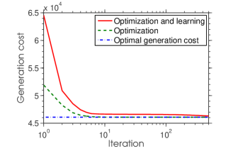
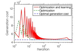
Figure 1: Strongly convex Opt. and learning: Const. steplength (l) and Diminish. steplength (r)

Figure 1 shows the behavior when using a constant steplength scheme, with $\gamma_{f}=0.04$ and $\gamma_{g}=0.003$. Note that the Lipschitz constants for the gradient of optimization and learning functions are $G_{f,x}=20$ and $G_{g}=250$, respectively, while the strong convexity constant of the optimization problem is $\eta_{f}=20$. Hence, the prescribed stepsizes satisfy the required conditions. The scheme is also compared to the case when using the optimal $\theta^{*}$ in the cost coefficient, requiring no learning. Expectedly, we observe slower convergence when the cost function coefficients are misspecified. The figure on the right displays the trajectories when using diminishing step length scheme with $\gamma_{f,k}=\gamma_{g,k}={1\over k}$. Figure  2 plots the convergence rate when using constant step size schemes and both the optimization and learning problems are strongly convex.

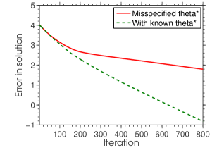
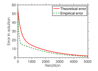
Figure 2: Strongly convex optimization: Impact on rate (l) and empirical vs. theor. rate (r)

Figure  2 (l) compares the error in solution iterates of optimization problem for the cases of missipecified and known $\theta^{*}$. As would be expected, when no learning is involved, we observe a linear convergence rate as shown in the dashed line. However, when learning is incorporated, the rate drops as shown by solid line. Figure  2 (r) compares the actual error in solution iterates of misspecified optimization problem to the theoretically predicted bound obtained in Proposition  4 and supports the validity of the bound.

No. of generators	Constant step size, $k=5000$		Diminishing step size, $k=15000$		Averaging scheme, $k=15000$
	$\|\theta_{k}-\theta^{*}\|$	$\frac{\|f(g_{k},\theta^{*})-f^{*}\|}{1+f^{*}}$	$\|\theta_{k}-\theta^{*}\|$	$\frac{\|f(g_{k},\theta^{*})-f^{*}\|}{1+f^{*}}$	$\|\theta_{k}-\theta^{*}\|$	$\frac{\|f(g_{k},\theta^{*})-f^{*}\|}{1+f^{*}}$
5	$3.3$$e$-$3$	$9.4$$e$-$7$	$1.3$$e$-$3$	$5.7$$e$-$4$	$6.9$$e$-$7$	$3.4$$e$-$4$
10	$1.2$$e$-$2$	$2.7$$e$-$6$	$2.7$$e$-$3$	$6.0$$e$-$4$	$1.1$$e$-$6$	$5.8$$e$-$4$
15	$1.2$$e$-$1$	$5.4$$e$-$5$	$1.2$$e$-$3$	$5.9$$e$-$4$	$2.1$$e$-$6$	$5.6$$e$-$4$
20	$9.0$$e$-$1$	$3.0$$e$-$3$	$4.3$$e$-$2$	$1.2$$e$-$3$	$5.0$$e$-$6$	$6.6$$e$-$4$

Table 4: Constant and diminishing stepsize and averaging schemes

In Table 4, we examine the performance of the various schemes as the problem size grows. The implemented schemes are the constant step size scheme proposed in Proposition 2 , diminishing step size scheme proposed in Proposition 3 and averaging scheme stated in proposition 6. We compare the error in both the solution to the learning problem and the error in the function value associated with the optimization problem after a prescribed set of iterations. While constant steplength schemes perform well, the performance appears to be more affected by problem size in comparison with diminishing steplength or averaging schemes. This can be traced to the observation that as problem size grows, the Lipschitz constant of gradient of learn function increases as well and the employed step sizes for constant step size scheme are adjusted accordingly.

Figure  3 displays the performance when using the averaging schemes proposed in Proposition  6. With known $\theta^{*}$, the rate of convergence in function values is of the order of $1/K$ where $K$ is number of steps. In Figure  3 (l), the error in function values is shown as a dashed line when $\theta^{*}$ is known and this rate drops by a constant factor when learning is involved as shown by the solid line. Figure  3 (r) compares the theoretical bound in Proposition  6 with the empirical error. As it is confirmed in this figure, the theoretically predicted rate represents an upper bound to the actual convergence rate of averaging scheme. Table  4 displays the errors obtained from running the averaging scheme for $15000$ iterations with increasing number of generators.

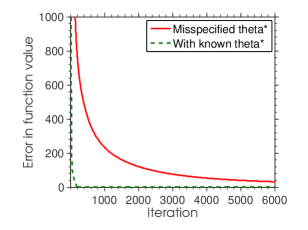
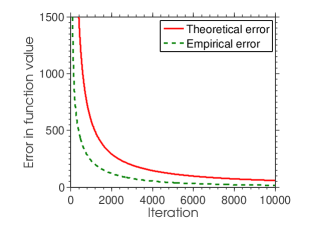
Figure 3: Convex optimization: Impact on rate (l) and empirical vs. theor. (r)

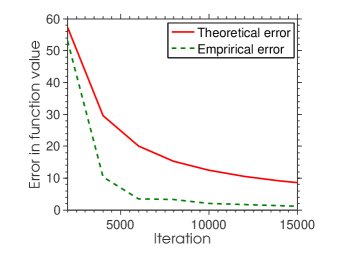
Figure 4: Nonsmooth convex optimization: empirical error vs. theor. bound

To test the joint subgradient scheme(Algorithm 2), we consider a nonsmooth generation cost function that is the maximum of $3$ linear functions and is defined as below:

$$c_{i}(g;\theta_{i})=\max\Big{(}\theta_{i1}g+\theta_{i2},\theta_{i3}g+\theta_{i4},\theta_{i5}g+\theta_{i6}\Big{)}\quad i=1,\dots,N$$

Figure  4 displays the result using the optimal constant step length scheme proposed in part (ii) of Proposition  14. Given a terminal iteration index $K$, the optimal step length is first calculated using  (24) and then the scheme is terminated after $K$ number of iterations. Figure  4 compares the resulted empirical error in function value of averaged point versus the theoretical bound. As shown in the figure, the empirical error is within the theoretical bound.

4.3 Misspecified demand

Suppose that demand vector $d\triangleq(d_{t}:t=1,\ldots,T)$ is misspecified and may be learnt through a parallel learning process. We refer to the misspecifed problem as (EDisp$(d)$) where $d$ denotes the misspecified demand. Suppose the linear inequality constraints of (EDisp$(d)$) are given by

$$h(g)\triangleq\begin{pmatrix}\begin{pmatrix}\sum_{i=1}^{N}g_{i,t}-d^{*}_{t}\end{pmatrix}_{t=1}^{T}\\ \begin{pmatrix}G_{i}-g_{i,t}\end{pmatrix}^{T}_{i,t=1}\\ \begin{pmatrix}{r}^{\rm up}_{i}-g_{i,t}+g_{i,t-1}\end{pmatrix}_{i,t=2}^{T}\\ \begin{pmatrix}{r}^{\rm down}_{i}-g_{i,t-1}+g_{i,t}\end{pmatrix}_{i,t=2}^{T}\end{pmatrix},$$

where $g\triangleq(g_{i,t}:i=1,\ldots,N$, $t=1,\ldots,T)$, and the cost function is given by $c(g)\triangleq\sum_{t=1}^{T}\sum_{i=1}^{N}c_{i}(g_{i,t})$. The first order conditions of this problem are necessary and sufficient and are given by

$$0\leq z\perp F(z;d^{*})\geq 0,\mbox{ where }z\triangleq\begin{pmatrix}g\\ \lambda\end{pmatrix},F(z)\triangleq\begin{pmatrix}\nabla_{g}c(g;d^{*})-\nabla_{g}h(g;d^{*})^{T}\lambda\\ h(g;d^{*})\end{pmatrix},$$

and $\lambda$ is a vector of dual variables corresponds to the constraints set $h(g)\geq 0$. The above conditions can be compactly stated as VI$(Z,F(\bullet;d^{*}))$ [13] allowing us to consider the use of the regularized and extragradient schemes developed in Section  3 for the solution of misspecified variational inequality problems. We consider a set of $5$ generators with known quadratic cost functions while the demand vector $d^{*}=(d^{*}_{t}:t=1,\ldots,T)$ is unknown. A set of $1000$ samples is randomly generated and the optimal demand is the solution to the following learning problem:

$$\min_{d\in\mathbb{R}_{+}^{T}}L(d)\quad\mbox{where}\quad L(d)\triangleq\sum_{i=1}^{1000}\|d-y_{i}\|^{2},$$

and $y_{i}$, $i=1,\ldots,1000$ denote the set of samples. Since the variational problem is merely monotone, the solution set is multi-valued. In such settings, we use the gap function [10] as a metric of progress, which is analogous to the objective function in optimization. Given VI$(Z,F)$, associated gap function is defined as follows:

$$G(y)\triangleq\begin{cases}F(y)^{T}y,&F(y)\in{Z}^{\circ}\\ +\infty,&F(y)\not\in Z^{\circ},\end{cases}$$

where ${Z}^{\circ}\triangleq\left\{z:z^{T}y\geq 0,y\in Z\right\}.$ Recall that $x$ solves VI$(Z,F)$ if and only if $G(x)=0$. To allow for representing the gap function when $F(y)\not\in{Z}^{\circ}$, we use a modified gap function given by $G(y)=F(y)^{T}y$, which could be negative. Figure  5 (l) compares the trajectory of gap function value with learning (solid line) with the trajectory observed when $d^{*}$ is available. Note that in this problem, $T=2$ and $\gamma_{f}={k^{-0.65}}$ and $\epsilon_{k}={k^{-0.34}}$. In addition, we employ a constant step size of $\gamma_{g}=.003$ for the learning problem, given that the Lipschitz constant of $\nabla_{d}L(d)$ is estimated to be $520$. Expectedly, learning leads to a degradation in the convergence rate as compared with using the true demand $d^{*}$. In Figure  5 (r), we examine the behavior of the misspecified extragradient scheme where $T=5$ and $L_{F,x}=2.8$, $L_{F,\theta}=1$ and $G_{g}=2$, respectively. Hence, the step sizes are fixed at $\tau=0.01$ and $\gamma_{g}=0.9$. Finally, in Table 5, we examine the error when the number of generators increases. We terminate the regularized and extragradient scheme after $10000$ and $150000$ iterations and we present the error in solution iterates of learning function as well as the gap function associated with the true problem. Since the extragradient scheme is a constant steplength scheme, its performance appears to be significantly better than the regularized scheme but the latter does not necessitate knowledge of system parameters.

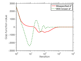
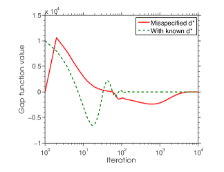
Figure 5: Monotone VIs: Regularized schemes (l) and Extragradient schemes (r)

No. of generators	Extragradient scheme, $k=10000$		Regularization scheme, $k=150000$
	$\|d_{k}-d^{*}\|$	G$(g_{k};d^{*})$	$\|d-d^{*}\|$	G$(g_{k};d^{*})$
5	$4.5$$e$-$6$	$2.10$$e$-$5$	$2.7$$e$-$4$	$1.2$$e$-$3$
10	$9.8$$e$-$6$	$4.36$$e$-$5$	$3.8$$e$-$4$	$2.3$$e$-$3$
15	$1.3$$e$-$5$	$6.5$$e$-$5$	$4.6$$e$-$4$	$3.4$$e$-$3$
20	$1.8$$e$-$5$	$8.6$$e$-$5$	$5.3$$e$-$4$	$4.5$$e$-$3$

Table 5: Convergence of extragradient and regularization schemes

5 Concluding remarks

The field of optimization algorithms has predominantly focused on the resolution of optimization problems when the objective function and the constraint set are known with certainty. However, in settings complicated by large networked systems with streaming data, the resulting optimization problems are often corrupted by a misspecification, either in terms of the model or a prescribed parameter. We focus on the second case and examine how one may resolve this misspecification through a suitably defined learning process. More precisely, we formalize the setting as one where we have two coupled computational problems; of these, the first is a misspecified optimization problem while the second is a learning problem that arises from having access to a learning data set, collected a priori. One avenue for contending with such a problem is through an inherently sequential approach that solves the learning problem and utilizes this solution in subsequently solving the computational problem. Unfortunately, unless accurate solutions of the learning problem are available in finite time, it appears that sequential approaches may not prove advisable.

In this paper, we consider a simultaneous approach that combines learning and computation via gradient-based techniques. We make several contributions in this regard, broadly categorized within the realm of misspecified convex optimization and monotone variational inequality problems: (i) Convex optimization problems: First, in strongly convex regimes, it can be readily shown that constant steplength gradient schemes admit global convergence properties. In regimes where the strong convexity constants are unavailable, we prove that suitably defined diminishing steplength schemes are also shown to be convergent. Furthermore, we provide rate statements that demonstrate a degradation the linear convergence rate, a consequence of incorporating learning. Next, we consider problems where the computational problem is merely convex and observe that both constant steplength gradient and subgradient methods see no change in the overall convergence rate but instead display a similar modification in their rates given by $\|\theta_{0}-\theta^{*}\|{\cal O}(q_{g}^{K}+1/K)$. This term is scaled by the initial misspecification in $\theta$ and comprises of two terms, the first being a term that emerges from learning the true $\theta^{*}$ and decays to zero at a geometric rate while the second is an interaction term that takes its rate from the averaging structure. When both the computation and the learning problems are assumed to be merely convex with an additional weak sharpness assumption on the learning problem, both constant steplength and diminshing steplength statements may be provided; (ii) Variational inequality problems: In the context of monotone variational inequality problems, we present two sets of techniques. Of these, the first is a constant steplength extragradient scheme in which the steplength bound is modified to incorporate the initial misspecification, given by $\|\theta_{0}-\theta^{*}\|$. Our second scheme develops an iterative (Tikhonov) regularized scheme that does rely on problem parameters and allows for recovery of the least norm solution of the misspecified variational inequality problem. Finally, preliminary numerical tests support the theoretical findings and remarkably the empirical convergence rates show a significant superiority to theoretical bounds, suggesting that improvements may be available.

Yet much remains to be understood about the realm of such techniques, For instance, to what extent does the introduction of learning affect the convergence rate in gradient methods as arising from Nesterov-type acceleration techniques? Furthermore, can be develop analogous rate statements for proximal and Lagrangian schemes and quantify the impacts from learning? Finally, can we extend this framework to other computational problems such as in the solution of Markov decision-making problems (MDPs)?

References

• [1] P. E. Gill, W. Murray, and M. H. Wright, Practical Optimization.   Boston, MA, USA: Academic Press, 1981.
• [2] D. Bertsekas, Nonlinear Programming: 2nd Edition.   Athena Scientific, Belmont, MA., 1999.
• [3] G. B. Dantzig, “Linear programming under uncertainty,” Management Sci., vol. 1, pp. 197–206, 1955.
• [4] E. M. L. Beale, “On minimizing a convex function subject to linear inequalities,” J. Roy. Statist. Soc. Ser. B., vol. 17, pp. 173–184; discussion, 194–203, 1955, (Symposium on linear programming.).
• [5] J. R. Birge and F. Louveaux, Introduction to Stochastic Programming: Springer Series in Operations Research.   Springer, 1997.
• [6] A. Shapiro, D. Dentcheva, and A. Ruszczyński, Lectures on stochastic programming, ser. MPS/SIAM Series on Optimization.   Philadelphia, PA: SIAM, 2009, vol. 9, modeling and theory. [Online]. Available: http://dx.doi.org/10.1137/1.9780898718751
• [7] A. Ben-Tal, L. El Ghaoui, and A. Nemirovski, Robust Optimization, ser. Princeton Series in Applied Mathematics.   Princeton University Press, October 2009.
• [8] D. Bertsimas, D. B. Brown, and C. Caramanis, “Theory and applications of robust optimization,” SIAM Rev., vol. 53, no. 3, pp. 464–501, Aug. 2011. [Online]. Available: http://dx.doi.org/10.1137/080734510
• [9] T. Hastie, R. Tibshirani, and J. H. Friedman, The elements of statistical learning: data mining, inference, and prediction: with 200 full-color illustrations.   New York: Springer-Verlag, 2001.
• [10] F. Facchinei and J.-S. Pang, Finite-dimensional variational inequalities and complementarity problems. Vol. I, ser. Springer Series in Operations Research.   New York: Springer-Verlag, 2003.
• [11] J. C. Gittins, Multi-armed bandit allocation indices.   Wiley-Interscience Series in Systems and Optimization, Chichester: John Wiley & Sons, Ltd., 1989.
• [12] H. Jiang and U. V. Shanbhag, “On the solution of stochastic optimization and variational problems in imperfect information regimes,” http://arxiv.org/abs/1402.1457, 2014.
• [13] F. Facchinei and J. S. Pang, Finite-dimensional variational inequalities and complementarity problems. Vol. I, ser. Springer Series in Operations Research.   New York: Springer-Verlag, 2003.
• [14] G. C. Calafiore and M. C. Campi, “Uncertain convex programs: Randomized solutions and confidence levels,” Mathematical Programming, vol. 102, pp. 25–46, 2005.
• [15] M. N. Katehakis and A. F. Veinott, “The multi-armed bandit problem: Decomposition and computation,” Mathematics of Operations Research, vol. 12, no. 2, pp. 262–268, 1987. [Online]. Available: http://dx.doi.org/10.1287/moor.12.2.262
• [16] S. Agrawal, Z. Wang, and Y. Ye, “A dynamic near-optimal algorithm for online linear programming,” Operations Research, vol. 62, no. 4, pp. 876–890, 2014.
• [17] S. Agrawal, E. Delage, M. Peters, Z. Wang, and Y. Ye, “A unified framework for dynamic prediction market design,” Operations Research, vol. 59, no. 3, pp. 550–568, 2011.
• [18] Z. Wang, S. Deng, and Y. Ye, “Close the gaps: A learning-while-doing algorithm for single-product revenue management problems,” Operations Research, vol. 62, no. 2, pp. 318–331, 2014.
• [19] H. Jiang, U. V. Shanbhag, and S. P. Meyn, “Distributed computation of equilibria in misspecified convex stochastic Nash games,” http://arxiv.org/abs/1308.5448, 2013.
• [20] D. Bertsekas and J. N. Tsitsiklis, “Gradient convergence in gradient methods with errors,” SIAM J. on Optimization, vol. 10, no. 3, pp. 627–642, Jul. 1999. [Online]. Available: http://dx.doi.org/10.1137/S1052623497331063
• [21] A. d’Aspremont, “Smooth optimization with approximate gradient,” SIAM J. on Optimization, vol. 19, no. 3, pp. 1171–1183, Oct. 2008. [Online]. Available: http://dx.doi.org/10.1137/060676386
• [22] D. Olivier, G. François, and Y. E. Nesterov, “First-order methods of smooth convex optimization with inexact oracle,” Math. Program., Ser. A, 03/2013 2013.
• [23] I. Necoara and V. Nedelcu, “Rate analysis of inexact dual first-order methods application to dual decomposition,” IEEE Transactions on Automatic Control, vol. 59, no. 5, May 2014.
• [24] M. Schmidt, N. L. Roux, and F. R. Bach, “Convergence rates of inexact proximal-gradient methods for convex optimization,” in Advances in Neural Information Processing Systems 24, J. Shawe-Taylor, R. Zemel, P. Bartlett, F. Pereira, and K. Weinberger, Eds.   Curran Associates, Inc., 2011, pp. 1458–1466.
• [25] D. S. Kirschen and G. Strbac, Fundamentals of Power System Economics.   John Wiley & Sons, 2004.
• [26] B. T. Polyak, Introduction to optimization.   New York: Optimization Software, Inc., 1987.
• [27] D. Bertsekas, A. Nedić, and A. E. Ozdaglar, Convex analysis and optimization.   Athena Scientific, Belmont, MA, 2003.
• [28] H. Robbins and D. Siegmund, “A convergence theorem for non negative almost supermartingales and some applications,” in Optimizing methods in statistics (Proc. Sympos., Ohio State Univ., Columbus, Ohio, 1971).   New York: Academic Press, 1971, pp. 233–257.
• [29] S. Boyd and L. Vandenberghe, Convex Optimization.   New York, NY, USA: Cambridge University Press, 2004.
• [30] G. M. Korpelevich, “The extragradient method for finding saddle points and other problems.” Ekonomika i Matematischeskie Metody, vol. 12, p. 747–756, 1976.
• [31] A. Nemirovski, “Prox-method with rate of convergence O(1/T) for variational inequalities with lipschitz continuous monotone operators and smooth convex-concave saddle point problems,” SIAM J. on Optimization, vol. 15, no. 1, pp. 229–251, Jan. 2005.
• [32] F. Facchinei and J. S. Pang, Finite-dimensional variational inequalities and complementarity problems. Vol. II, ser. Springer Series in Operations Research.   New York: Springer-Verlag, 2003.
• [33] A. N. Tikhonov, “On the solution of incorrectly put problems and the regularisation method,” in Outlines Joint Sympos. Partial Differential Equations (Novosibirsk, 1963).   Acad. Sci. USSR Siberian Branch, Moscow, 1963, pp. 261–265.
• [34] A. N. Tikhonov and V. Arsénine, Méthodes de resolution de problèmes mal posés.   Moscow: Éditions Mir, 1976, traduit du russe par Vladimir Kotliar.
• [35] E. G. Golshtein and N. V. Tretyakov, Modified Lagrangians and monotone maps in optimization, ser. Wiley-Interscience Series in Discrete Mathematics and Optimization.   New York: John Wiley & Sons Inc., 1996, translated from the 1989 Russian original by Tretyakov, A Wiley-Interscience Publication.
• [36] A. Kannan and U. V. Shanbhag, “Distributed computation of equilibria in monotone Nash games via iterative regularization techniques.” SIAM Journal on Optimization, vol. 22, no. 4, pp. 1177–1205, 2012.