Anomalous surface states at interfaces in p-wave superconductors

Abstract

We present the results of theoretical study of surface state properties in a two-dimensional model for triplet $p$-wave superconductors. We derive boundary conditions for Eilenberger equations at rough interfaces and develop the approach for self-consistent solution for the spatial dependence of $p_{x}$ and $p_{x}+i~{}p_{y}$ -wave pair potentials. In the $p_{x}$ case we demonstrate the robustness of the zero-energy peak in the density of states (DoS) with respect to surface roughness, in contrast to the suppression of such a peak in the case of $d_{xy}$ symmetry. This effect is due to stability of odd-frequency pairing state at the surface with respect to disorder. In the case of the chiral $p_{x}+i~{}p_{y}$ state we demonstrate the appearance of a complex multi-peak subgap structure in the spectrum with increasing surface roughness.

I Introduction

Investigation of spin-triplet superconductivity is currently an exciting topic of research by the superconducting community. There are several experimental results in Sr₂RuO₄ Maeno ; Ishida ; Luke ; Mackenzie ; Nelson ; Asano and in heavy fermion compounds Tou ; Muller ; Qian ; Abrikosov ; Fukuyama ; Lebed ; Saxena ; Peiderer ; Aoki that are consistent with spin-triplet superconducting pairing. The promising paring symmetries are believed to be $p$-wave and $f$-wave in Sr₂RuO₄ Maeno ; Ishida ; Luke ; Mackenzie ; Kikugawa and UPt₃ Graf ; Machida ; Lussier , respectively. Furthermore, to design $p$-wave superconductivity based on a proximity coupled system with a conventional $s$-wave superconductor and the semiconductor surface state of a topological insulator Alicea1 ; Sau1 ; Sau2 ; Yamakage ; Fu ; akhmerov09 ; tanaka09 ; Law ; Lutchyn ; Oreg has become a hot topic from the viewpoint of topological superconductivity Ryu ; Aliceareview ; Qi ; Nagaosa . The essential ingredients in these new systems are momentum-spin locking due to spin-orbit coupling and time reversal symmetry breaking by an external field.

In the above systems, it is known that surface Andreev bound state (SABS) Buchholtz ; Hara ; Hu ; Kashiwaya ; Yada is generated inside the energy gap and stems from the topological properties of the bulk Hamiltonian Sato2011 . The SABS has become a prominent concept since the debate over the pairing symmetry of high temperature superconductors (HTSs) Hu ; Tanaka1 . In HTSs, if the angle between the direction normal to the surface and the lobe direction of the $d$-wave pair potential deviates from zero, the injected quasiparticle and the reflected one can feel opposite signs of the pair potential depending on the injection angle Tanaka1 . The extreme case is that the above angle becomes $\pm\pi/4$, where an injected quasiparticle always feels the sign change independent of the injection direction. This sign change of the pair potential produces SABS at zero energy and induces the zero bias conductance peak in tunneling spectroscopy Tanaka1 ; Kashiwaya ; Lofwander . The SABS has a flat dispersion along $k_{y}$, where $k_{y}$ is the momentum parallel to the surface. Actually, there are many experimental reports supporting ZBCP stemming from SABS Kashiwayaexp ; Covington ; Alff ; Wei ; Iguchi ; Biswas ; Chesca .

When the zero energy SABS is located at the surface or interface, suppression of the pair potential in the main pairing channel occurs Nagato ; Buchholtz95 ; Barash ; Tanuma98 . Furthermore, if the time reversal symmetry breaking is induced by the surface subdominant pair potential, ZBCP can split Matsumoto95 ; Fogelstrom ; Covington ; Tanuma01 . Thus, experimental study of the properties of ZBCP can serve as a guide to determine the symmetry of the pair potential and the possible presence of a subdominant one near the surface.

At the actual surface or interface, the diffusive scattering by the roughness due to atomic scale irregularity inevitably exists. It is known that surface roughness influences the electronic states of unconventional superconductors such as those of $d$-wave or $p$-wave type Buchholtz86 ; WZhang ; NagatoLTP . Studies of conductivity at the interfaces in $d$-wave superconductors have shown that their properties are strongly influenced by the degree of diffusive scattering of quasiparticles at the interface Barash ; Fogelstrom ; Golubov1 ; Golubov1b ; Golubov2 . The higher the intensity of the diffusive scattering, the less pronounced the conductance peak at low voltages and the more pronounced the influence of subdominant components of order parameter on its shape.

Besides the above mentioned works, the theory of a proximity effect in diffusive normal metal / $d$-wave superconductor junctions has been developed Nazarov . It has been clarified that SABS can not penetrate into diffusive normal metal (DN) and the resulting ZBCP is broadened. These properties can be naturally explained using the concept of odd-frequency pairing Berezinskii . The odd-frequency pairing states such as spin-singlet $p$-wave or spin-triplet $s$-wave can be generated by the translational symmetry breaking from the bulk conventional even-frequency pairing state, $e.g.$, spin-singlet $s$($d$)-wave or spin-triplet $p$-wave Tanaka6 ; Eschrig07 . It is revealed that SABS in $d$-wave superconductor might be interpreted as an odd-frequency spin-singlet $p$-wave pairing Tanaka6 ; Tanaka07 . However, $p$-wave pairing is fragile against diffusive scattering, so it can not penetrate into DN metal. This property is consistent with the fact that surface roughness has strong effect on ZBCP and SABS in $d$-wave superconductor.

On the other hand, a recent study of SBAS in $p$-wave superconductors has been stimulated by investigation of pairing symmetry in Sr₂RuO₄. The existing theory of the proximity effect in spin-triplet $p$-wave superconductors predicts that SABS produced by $p_{x}$-wave pairing can penetrate into DN metal attached to a spin-triplet $p_{x}$-wave superconductor Tanaka4 . This proximity effect induces many exotic phenomena including a zero enegy peak in the local density of state (LDoS) and negative local superfluid density Tanaka5 ; Tanaka2006 ; Asano2007 ; Fominov ; Asano11 ; Higashitani13 ; Keles . Since the SBAS in a spin-triplet $p$-wave superconductor corresponds to odd-frequency spin-triplet $s$-wave pairing, it is robust against impurity scattering Tanaka07 .

In actual Sr₂RuO₄, the promising symmetry is chiral $p$-wave pairing, $i.e.$, $p_{x}+ip_{y}$ and one can expect more complex state as compared to $p_{x}$-wave or $d_{xy}$-wave cases. The resulting SABS has a linear dispersion as a function of $k_{y}$ Matsumoto99 ; Furusaki which is different from SABS in spin-singlet $d$-wave or spin-triplet $p_{x}$-wave superconductor. For a ballistic junction without any roughness, it has been shown that the resulting conductance exhibits a wide variety of line shapes including broad ZBCP or dip like structure around zero voltage Yamashiro ; Honerkamp ; Sengupta ; Laube . Although it is not easy to obtain reliable tunneling spectroscopy data in the $ab$-plane junction experimentally, recent fabrication of well oriented junctions enabled detection of the SABS Kashiwaya11 . However, the effect of diffusive scattering has not been clarified yet. For a detailed comparison with experiment and predicted surface state, the research in this direction is needed. Since there are several relevant works in the surface state of superfluid ³He Higashitani ; Higashitani2 , it is currently a challenging issue to study surface roughness effect on the surface density of states (SDoS) and pairing symmetry of chiral $p$-wave superconductors.

Despite the fact that previous studies revealed important aspects of these phenomena Zhang ; Matsumoto2 ; Nagato3 , there is still a need for systematic study and quantitative predictions. The purpose of this study is to evaluate the influence of the degree of diffusive electron scattering at interfaces in $p$-wave superconductors on the DoS.

The structure of this paper is the following: in Section II we formulate the problem and derive effective boundary conditions for diffusive surfaces in $p$-wave superconductors. In the following sections we discuss microscopic properties of pairing in such systems for the cases of both $p_{x}$ and chiral $p_{x}+ip_{y}$ symmetry. In the Sec.III we focus on the spatial dependence of pair potential $\Delta$; Sec.IV is devoted to pair amplitudes $f$ and finally in Sec.V we consider DoS for various surface properties.

II Model

The description of the suppression of superconductivity in the main pairing channel and of the generation of subdominant order parameters can be done within the framework of the quasiclassical Eilenberger equations Eilenberger within a two-dimensional model. To solve the problem, we will assume that the conditions of the clean limit are valid in the bulk superconductor region (scattering time $\tau\rightarrow\infty$ ) and the equations have the form

$$2\omega f(x,\theta)+v\cos(\theta)\frac{d}{dx}f(x,\theta)=2\Delta g(x,\theta),$$ (1)

$$2\omega f^{+}(x,\theta)-v\cos(\theta)\frac{d}{dx}f^{+}(x,\theta)=2\Delta^{\ast}g(x,\theta),$$ (2)

$$2v\cos(\theta)\frac{d}{dx}g_{\omega}(x,\theta)=2\left(\Delta^{\ast}f_{\omega}-\Delta f_{\omega}^{+}\right).$$ (3)

Here $g(x,\theta)$, $f(x,\theta)$ and $\ f^{+}(x,\theta)$ are normal and anomalous Eilenberger functions, $\Delta(x)$ is pair potential, $\theta$ is angle between the vector normal to the interface and the direction of the electron Fermi velocity $v;$ $\omega=\pi T(2n+1)$ are Matsubara frequencies and $T$ is temperature, $x$ is coordinate along the axis normal to the boundary. The form of self-consistency equation is sensitive to the chosen symmetry of pair potential. In the case of $p_{x}$-wave pairing potential $\Delta=\Delta_{x}\cos(\theta)$ leads to equation

$$\Delta_{x}\ln\frac{T}{T_{c}}+2\pi T\sum_{\omega}\frac{\Delta_{x}}{\omega}-\left\langle 2\cos(\theta^{\prime})~{}f(x,\theta^{\prime})\right\rangle=0.$$ (4)

The other type of chiral $p_{x}+i~{}p_{y}$ symmetry relates to $\Delta=\Delta_{x}\cos(\theta)+i~{}\Delta_{y}\sin(\theta)$ with similar self-consistent equation Bruder

$$\Delta_{x}\ln\frac{T}{T_{c}}+2\pi T\sum_{\omega}\frac{\Delta_{x}}{\omega}-\left\langle 2\cos(\theta^{\prime})Ref(x,\theta^{\prime})\right\rangle = 0,$$ (5)

$$\Delta_{y}\ln\frac{T}{T_{c}}+2\pi T\sum_{\omega}\frac{\Delta_{y}}{\omega}-\left\langle 2\sin(\theta^{\prime})Imf(x,\theta^{\prime})\right\rangle = 0.$$ (6)

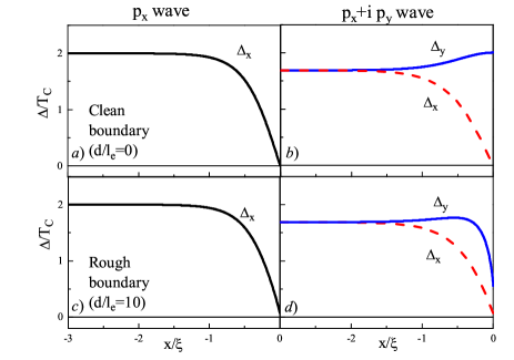
Figure 1: Pair potential $\Delta$ as a function od coordinate $x$ in the vicinity of surface for a) $p_{x}$-wave superconductor with clean surface, b) $p_{x}+ip_{y}$-wave superconductor with clean surface, a) $p_{x}$-wave superconductor with rough surface, a) $p_{x}+ip_{y}$-wave superconductor with rough surface. On the panels b) and d) solid and dashed lines correspond to components $\Delta_{y}$ and $\Delta_{x}$ respectively. Tha parameter $d/l_{e}$ determines the degree of the surface roughness.

Here $\left\langle...\right\rangle=(1/2\pi)\int_{0}^{2\pi}(...)d\theta$ and $T_{c}$ is the critical temperature. Note that the considered case of chiral p-wave supercondutor is equivalent to a thin film of superfluid 3He A-phase. The polar phase of 3He has been recently identified in aerogel 3He1 ; 3He2 .

Diffusive properties of the interface will be described in the Ovchinnikov model Ovchinnikov , i.e. it is simulated by a thin diffusive layer of thickness, $d\ll\xi_{eff}=\min\left\{\sqrt{\xi_{0}l_{e}},\ \xi_{0}\right\},$ $\xi_{0}=v/2\pi T_{c},$ with strong electron scattering inside. Here $l_{e}$ is electron mean free path and $\tau=l_{e}/v$. Inside this layer, located in the area $0\leq x\leq d$, we can neglect terms in the Eilenberger equations Eilenberger that are proportional to $\omega$ and $\Delta$

$$v\cos(\theta)\frac{d}{dx}f(x,\theta)=\frac{1}{\tau}\left(g\left\langle f\right\rangle-f\left\langle g\right\rangle\right),$$ (7)

$$v\cos(\theta)\frac{d}{dx}f^{+}(x,\theta)=\frac{1}{\tau}\left(g\left\langle f^{+}\right\rangle-f^{+}\left\langle g\right\rangle\right),$$ (8)

$$2v\cos(\theta)\frac{d}{dx}g(x,\theta)=\frac{1}{\tau}\left(f\left\langle f^{+}\right\rangle-f^{+}\left\langle f\right\rangle\right)$$ (9)

and assume that $\left\langle f\right\rangle$, $\left\langle f^{+}\right\rangle$ and $\left\langle g\right\rangle$ are spatially independent quantities, which should be determined selfconsistently during the process of finding solutions of the system (1)-(9). For the development of numerical algorithms for solving the Eilenberger equations it is convenient to rewrite them using the Ricatti parametrization Schopohl ; Tanaka6 .

$$f_{\pm}=\frac{2a_{\pm}}{1+a_{\pm}b_{\pm}},\ f_{\pm}^{+}=\frac{2b_{\pm}}{1+a_{\pm}b_{\pm}},\ g_{\pm}=\frac{1-a_{\pm}b_{\pm}}{1+a_{\pm}b_{\pm}},$$ (10)

that are defined in the angle $-\pi/2\leq\theta\leq\pi/2.$ Their substitution into (1)-(9) leads to the general relations in the form

$$v\cos(\theta)\frac{d}{dx}a_{\pm} = \Delta\left[1-a_{\pm}^{2}\right]\mp 2\omega a_{\pm}$$ (11)

$$v\cos(\theta)\frac{d}{dx}b_{\pm} = -\Delta\left[1-b_{\pm}^{2}\right]\pm 2\omega b_{\pm}$$ (12)

in the clean superconducting region and

$$v\cos(\theta)\frac{d}{dx}a_{\pm} = \pm\frac{1}{2\tau}\left[\left\langle f\right\rangle-a_{\pm}^{2}\left\langle f^{+}\right\rangle-2a_{\pm}\left\langle g\right\rangle\right]$$ (13)

$$v\cos(\theta)\frac{d}{dx}b_{\pm} = \mp\frac{1}{2\tau}\left[\left\langle f^{+}\right\rangle-b_{\pm}^{2}\left\langle f\right\rangle-2b_{\pm}\left\langle g\right\rangle\right]$$ (14)

in the diffusive layer. The subscript $\pm$ indicates the direction of motion along the trajectory towards the boundary $(+)$ or away from it $(-)$. For $x\rightarrow-\infty$ we have

$$a_{\pm}=\pm\frac{\Delta}{\omega+\sqrt{\omega^{2}+|\Delta|^{2}}},$$ (15)

$$b_{\pm}=\pm\frac{\Delta^{\ast}}{\omega+\sqrt{\omega^{2}+|\Delta|^{2}}},$$ (16)

where $\Delta$ is the bulk value of pair potential.

Finally, the problem must be supplemented by boundary conditions at the free surface of the diffusion layer $(x=d)$

$$b_{+}(d,-\theta)=b_{-}(d,\theta),$$ (17)

$$a_{-}(d,-\theta)=a_{+}(d,\theta).$$ (18)

The boundary conditions (17), (18) differ significantly from those used previously Golubov2

$$b_{+}(d,-\theta)=a_{+}(d,\theta),$$ (19)

in the analysis of the influence of diffuse scattering on the superconducting correlations in $d$-wave superconductors. Indeed, in the $d$-wave case the following relations

$$b_{\pm}(x,\theta)=a_{\mp}(x,\theta),$$ (20)

hold, and then the conditions (17), (18) are reduced to the relation (19). As a result, further analysis in the $d$-wave case was based not on four, but only on two Eilenberger functions. It should be also pointed out that when writing conditions (17-18) we essentially used not only the fact that the particle reflected from the free surface must diffuse into the node with a opposite value of the order parameter, but also the fact that its velocity should be directed into the interior of superconductor. That is why in the right side of (17) there is a function $b_{-}(d,\theta)$, and there is not $a_{+}(d,\theta)$, or some combination of them.

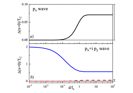
Figure 2: Pair potential $\Delta$ on a surface of diffusive layer versus its roughness $d/l_{e}$ a) for $p_{x}$-wave superconductor and b) $p_{x}+ip_{y}$-wave superconductor. Solid and dashed lines on the panel b) correspond to components $\Delta_{y}$ and $\Delta_{x}$ respectively.

The boundary value problem (11)-(18) has been solved analytically (see Appendix) resulting in an effective boundary condition at the interface between the clean $p$-wave area and the diffusive layer at the $x=0$. It is expressed as the relation between the functions of a coming into the diffusive layer $a_{+}(0,-\theta)$, $b_{-}(0,-\theta)$ and leaving out from it $a_{-}(0,\theta)$, $b_{+}(0,\theta)$.

$$a_{-}(0,\theta)=\frac{a_{+}(0,-\theta)-\left(Ga_{+}(0,-\theta)-F\right)\tanh\left\{kd\right\}}{\left(F^{+}a_{+}(0,-\theta)+G\right)\tanh\left\{kd\right\}+1},$$ (21)

$$b_{+}(0,\theta)=\frac{b_{-}(0,-\theta)-\left(Gb_{-}(0,-\theta)-F^{+}\right)\tanh\left\{kd\right\}}{\left(Fb_{-}(0,-\theta)+G\right)\tanh\left\{kd\right\}+1}.$$ (22)

Here $k$ is an effective wave vector in dirty layer

$$k=\frac{\sqrt{\left\langle g_{+}+g_{-}\right\rangle^{2}+\left\langle f_{+}^{+}+f_{-}^{+}\right\rangle\left\langle f_{+}+f_{-}\right\rangle}}{\ell\cos(\theta)},$$ (23)

and $F$, $F^{+}$and $G$ are parametrized averages of Green functions

$$F = \frac{\left\langle f_{+}+f_{-}\right\rangle}{\sqrt{\left\langle g_{+}+g_{-}\right\rangle^{2}+\left\langle f_{+}^{+}+f_{-}^{+}\right\rangle\left\langle f_{+}+f_{-}\right\rangle}},$$ (24)

$$F^{+} = \frac{\left\langle f_{+}^{+}+f_{-}^{+}\right\rangle}{\sqrt{\left\langle g_{+}+g_{-}\right\rangle^{2}+\left\langle f_{+}^{+}+f_{-}^{+}\right\rangle\left\langle f_{+}+f_{-}\right\rangle}},$$ (25)

$$G = \frac{\left\langle g_{+}+g_{-}\right\rangle}{\sqrt{\left\langle g_{+}+g_{-}\right\rangle^{2}+\left\langle f_{+}^{+}+f_{-}^{+}\right\rangle\left\langle f_{+}+f_{-}\right\rangle}}.$$ (26)

Here the averaging operation is performed over the range of angles, $-\pi/2\leq\theta\leq\pi/2,$ that is $\left\langle...\right\rangle=(1/2\pi)\int_{-\pi/2}^{\pi/2}(...)d\theta.$

The above boundary conditions are the main analytical result of this paper and they provide the framework for a quantitative selfconsistent study of surface effects in $p$-wave superconductors. The results of this study are presented below.

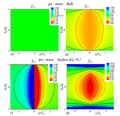
Figure 3: (Color Online) Odd and even angle resolved pairing amplitudes $f_{1}$ and $f_{2}$ as functions of $k_{y}$ and $\omega$ a), b) in the bulk $p_{x}$-wave superconductor and c),d) at the surface ($x=0$) with roughness $d/l_{e}=0.1$

III
Pair potential, $\Delta$

To study properties of the systems we have developed the method of numerical solution of the boundary-value problem (11)-(18). According to this method, outside of the diffusive layer (in the region where $(\tau\rightarrow\infty)$), the equations (11), (12) for $a_{+}(x,\theta)$ and $b_{-}(x,-\theta)$ are numerically integrated starting from conditions (15) at infinity $(x=-\infty)$ and moving along the trajectory towards the boundary $(x=0)$. As a result, functions $a_{+}(0,\theta)$ and $b_{-}(0,-\theta)$ in equations (21), (22) are calculated. Then, starting values $a_{-}(0,\theta)$ and $b_{+}(0,\theta)$ are determined from the boundary conditions (21), (22), and functions $a_{-}(x,\theta)$ and $b_{+}(x,\theta)$ are obtained by integration along the trajectories going out of the diffusive layer. The coefficients $F$, $F^{+}$ and $G$ in (21), (22) and the spatial dependence of the order parameter $\Delta(x)$ are determined in an iterative self-consistent way using Eqs. (21)-(26) and (4)-(6), respectively. All the calculations below were performed at temperature $T=0.5T_{C}$.

According to this procedure, we calculate spatial distributions of pair potential $\Delta(x)$, pair amplitude $f(x)$ and surface DoS (SDoS) for different thicknesses of diffusive layer.

Figure 1 shows spatial dependencies of the pair potential $\Delta(x)$ for $p_{x}$ and chiral $p_{x}+ip_{y}$ cases. In a $p_{x}$-wave superconductor, the amplitude of the pair potential $\Delta_{x}$ reaches its maximum value in the bulk ($\Delta_{x}\approx 2T_{C}$ at $T=0.5T_{C}$). In the vicinity of the interface it is suppressed up to zero in the absence of a diffusive layer. It comes from the fact that the reflection of electrons takes place into the band with negative sign of pair potential (See Fig. 1a). The presence of roughness does not change the general shape of the dependence and only provides slight growth of the pair potential $\Delta_{x}(0)$ at the surface (Figs. 1c and 2a).

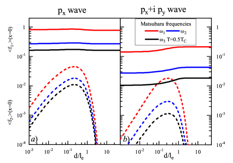
Figure 4: Odd $<f_{1}>$ and even $<f_{2}>$ components of pair amplitude at a surface ($x=0$) versus its roughness $d/l_{e}$. Panels a) and b) correspond to $p_{x}$-wave and to $p_{x}+ip_{y}$-wave respectively. Pair amplitudes are angle averaged and calculated for the first, the second and third Matsubara frequencies $\omega_{n}$ at temperature $T=0.5T_{C}$.

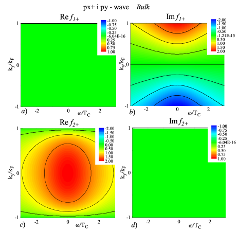
Figure 5: (Color Online) Odd and even angle resolved pairing amplitudes $f_{1}$ and $f_{2}$ in the bulk chiral superconductor as functions of $k_{y}$ and $\omega$.

For the case of chiral symmetry, the impact of surface is more diverse (See Fig. 1b,d). In contrast to the former case, the bulk pair potential has the BCS magnitude (for the considered temperature $\Delta_{x}=\Delta_{y}\approx 1.67T_{C}$) due to spherical symmetry of $\left|\Delta\right|$. As in the previous case, the component $\Delta_{x}$ is suppressed in the vicinity of a surface. In contrary, the component $\Delta_{y}$ grows up to the bulk value for $p_{y}$ symmetry in the case of a clean surface. However, $\Delta_{y}$ is sensitive to a degree of surface roughness: the pair potential component $\Delta_{y}$ decreases by about three times in comparison with bulk value in the limit of large roughness (Fig. 2b). This property has a simple qualitative explanation: in the clean limit the incident and reflected electrons fill the same sign of pair potential, while in the diffusive case some of the reflected electrons fills the opposite sign of the pair potential due to impurity scattering. In the following we will see that this phenomenon manifests itself in the DoS at a surface.

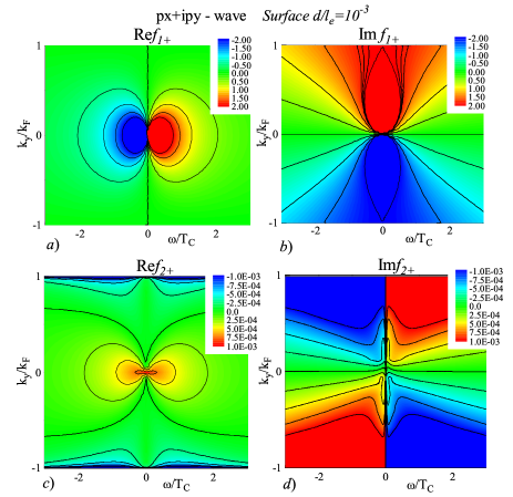
Figure 6: (Color Online) Odd and even angle resolved pairing amplitudes $f_{1}$ and $f_{2}$ as functions of $k_{y}$ and $\omega$ at the almost mirror surface ($x=0$) with roughness ($d/l_{e}=0.001$) for the chiral superconductor.

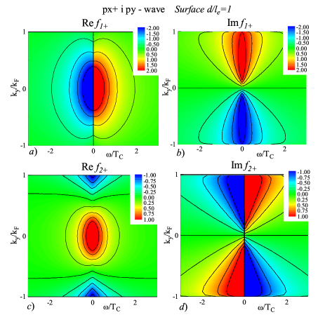
Figure 7: (Color Online) Odd and even angle resolved pairing amplitudes $f_{1}$ and $f_{2}$ as functions of $k_{y}$ and $\omega$ at the surface ($x=0$) with roughness ($d/l_{e}=1$) for the chiral superconductor.

IV
Pair amplitudes $f$ and $f^{+}$

An important characteristic of the considered system is a relation between surface roughness and the time-parity of the pairing amplitude $f$ near the surface. Let us introduce the symmetrized functions

$$f_{1\pm}=f_{\pm}-f_{\pm}^{+},$$ (27)

$$f_{2\pm}=f_{\pm}+f_{\pm}^{+}.$$ (28)

As follows from Eqs. (1)-(3) (see Appendix B), these Green functions have the following symmetries with respect to the Matsubara frequency:

$$g_{\omega}=-g_{-\omega}^{\ast};\ \ f_{1,\omega}=-f_{1,-\omega}^{\ast};~{}~{}f_{2,\omega}=f_{2,-\omega}^{\ast}$$ (29)

and with respect to the angle of motion $\theta$

$$f_{1}(\theta)=f_{1}^{\ast}(-\theta);~{}~{}f_{2}(\theta)=f_{2}^{\ast}(-\theta);~{}~{}g(\theta)=g^{\ast}(-\theta).$$ (30)

Such symmetry also means that imaginary parts of these functions are antisymmetric over $\theta$ and disappear after averaging over $\theta.$ Therefore, the average quantities $<f_{1,2}>$ are real functions and we can call function $<f_{1}>$ odd-frequency and $<f_{2}>$ even-frequency. To demonstrate this property, we trace the behavior of $<f_{1}>$ and $<f_{2}>$ in detail in the bulk superconductor and at the surface.

For a $p_{x}$-wave superconductor, the problem can be simplified and can be solved in terms of real values: the function $f_{1}(f_{2})$ is symmetric over angle $\theta$ and odd (even) over frequency $\omega$. We will focus on the functions $f_{1+}$ and $f_{2+}$ corresponding to incident trajectories. In the bulk superconductor only the even-frequency component $f_{2+}$ exists in full accordance with analytical solutions (15)-(16) (Fig. 3a,b). Hereinafter, we will present angle dependencies in terms of parallel component of the Fermi wave-vector $k_{y}=k_{F}\sin(\theta)$. At the surface the formation of another component takes place: electrons reflect into the lobe with different sign of order parameter (in accordance with Eqs. (17)-(18)) and an odd-frequency Green function $f_{1+}$ (Fig. 3c) is generated. Its amplitude diverges in the limit $\omega\rightarrow 0$, but remains finite at a certain Matsubara frequency $\omega_{n}$.

The behavior of even-frequency $f_{2+}$ is a quite complex. At the mirror surface it is fully destroyed by direct reflection of particles in accordance with Eqs. (17)-(18). Surface roughness leads to generation of even-frequency Green function $f_{2+}$ since reflected amplitudes $a_{-}$ and $b_{+}$ become isotropic. However the average value $\langle f_{1+}\rangle$ during further isotropization reaches its maximum and starts to decrease for larger roughness values (See Fig. 4a). This effect occurs because $f_{2+}$ has different signs at angles $\theta$ in the vicinity of $\pm\pi/2$ and $\theta=0$ and in the limit of a thick diffusive layer these angle areas compensate each other during integration.

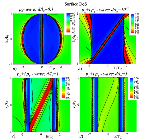
Figure 8: (Color Online) Surface $x=d$ angle-resolved DoS for a) $p_{x}$-wave with surface roughness $d/l_{e}=0.1$ and for b), c), d)$p_{x}+ip_{y}$-wave with roughness $d/l_{e}=10^{-3}$, $d/l_{e}=1$, $d/l_{e}=3$ respectively.

In the chiral $p_{x}+ip_{y}$ -wave superconductors the general properties of the Green functions are pretty similar: in the bulk all odd-frequency components of Green functions Re $f_{1}$ and Im $f_{2}$ don’t exist (Fig. 5a,d) and even ones correspond to the symmetry of real and imaginary parts of pair potential $\Delta$. Thus Re $f_{2+}$ has maximum at $\theta=0$, in accordance with the angle-dependence of $p_{x}$-component, and Im$f_{1+}$ reaches its maximum values at $\theta=\pi/2$ in accordance with $ip_{y}$-one. (Fig. 5b,c)

In the vicinity of the surface other components also arise. Particles reflected from the mirror boundary into the $p_{x}$-band with different sign of order parameter generate an odd-frequency pair amplitude. However, in imaginary values the sign of the $p_{y}$-component of the order parameter is conserved after reflection and hold even-frequency symmetry. Thus in this case there are only two significant components of Green functions: odd-frequency Re $f_{1+}$ with maximum at ($\theta=0$) and even-frequency Im $f_{1+}$ increasing for large angles. (See Fig. 6). In the structures with finite thickness of diffusive layer another Green function components arise. Isotropization of $a_{-}$ and $b_{+}$ leads to the formation of nonzero components Re $f_{2}$ and Im $f_{2}$. At greater roughness they increase further (Fig. 7), but the averaged value of $\left\langle f_{2+}\right\rangle$ falls down due to negative contribution from large angles.

To show this clearly we present angle averaged pair amplitudes $|\left\langle f_{1+}\right\rangle|$ and $|\left\langle f_{2+}\right\rangle|$ at the surface versus roughness (Fig. 4) for the first, the second and the third Matsubara frequencies at fixed temperature $T=0.5T_{C}$. Odd-frequency amplitude $|\left\langle f_{1+}\right\rangle|$ significantly exceeds even-frequency one $|\left\langle f_{2+}\right\rangle|$ in cases of both $p_{x}$ and chiral $p_{x}+ip_{y}$ symmetries. Furthermore, in limits of both low and high roughness the even-frequency component $|\left\langle f_{2+}\right\rangle|$ vanishes. At the same time , we have found that this component reaches its maximum value in the finite roughness range. This means that new effects exist in the range of intermediate roughness and one may expect a qualitative difference in measurable properties such as DoS in this regime.

V Density of States

To calculate DoS, one can solve the same system of equations (11)-(18), where Matsubara frequency is replaced by energy $\omega\rightarrow iE$. Further we will focus only on DoS for incident electrons because it is this quantity which is probed in tunnel experiments

$$DoS=Re(g_{+})=Re\left(\frac{1+a_{+}b_{+}}{1-a_{+}b_{+}}\right)$$ (31)

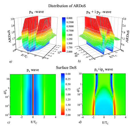
Figure 9: (Color Online) a,b) Spatial distribution of ARDoS ($\theta=0$) for the $p_{x}$-wave and $p_{x}+ip_{y}$-wave superconductors. c-d) Angle Averaged SDoS as a function of surface roughness.

Odd-frequency pairing around the surface leads to formation of subgap bound states, which occur as peaks in the angle resolved density of states (ARDoS) in both $p_{x}$ and $p_{x}+ip_{y}$ cases. Figure 8 shows ARDoS at the surface for $p_{x}$-wave (a) and for chiral superconductor (b, c, d) and reveals the behavior of the subgap bound states as a function of angle of propagation $\sin(\theta)$ and momentum $k_{y}$, respectively. In the $p_{x}$-case the peak is narrow and keeps its zero energy position for every $k_{y}$. The width of the gap is determined by the bulk pair potential $\Delta(\theta)=\Delta_{x}\cos(\theta)$ despite the pair potential at the surface is almost absent. Therefore, the predominant contribution to formation of ARDoS at the surface is provided by the proximity effect with the bulk superconductor.

In contrast, for the chiral symmetry case (Fig.8b-d), the energy of a bound state depends linearly on $k_{y}$. The dispersion of the corresponding peak depends on surface properties: the higher the roughness, the wider this peak. The value of the gap in the surface DoS is now $k_{y}$ independent and is also determined by proximity with the bulk material. However, for high $k_{y}$ (for the particles moving almost parallel to the surface) it grows up to $\Delta_{y}$ at the surface. In accordance with Fig. 1 it provides different properties in the limits of clean and rough surface since the value of $\Delta_{y}$ can be larger or smaller compared to the bulk. All these effects appear in the vicinity of the surface at distances of the order of coherence length (Fig. 9a-b).

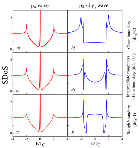
Figure 10: Angle Averaged Surface DoS for various values of the roughness parameter: ($d/l_{e}=0$ at the upper panels, $d/l_{e}=0.1$ at the middle panels and $d/l_{e}=1$ at the lower panels). Left and right columns of panels correspond to the $p_{x}$ and $p_{x}+ip_{y}$ symmetry, respectively

These properties lead to totally different angle averaged DoS for various symmetries. $p_{x}$ superconductor preserves the zero energy peak and peaks at the bulk $\Delta$ even in an averaged surface DoS (SDoS) regardless of the roughness (Fig. 10a,c,e). The results for the chiral case strongly depend on properties of the surface. In the case of mirror surface (Fig. 10b) angle-averaged subgap SDoS transforms into plateau with a value around zero. The structure above the gap includes two peaks: the intrinsic ($E=2T_{C}$) one provided by the surface component $\Delta_{y}$ of the pair potential and the proximity one ($E=1.67T_{C}$), which appears due to influence of the bulk part of material. However, the growth of roughness leads to suppression of $\Delta_{y}$ and to the shift of intrinsic peak inside the energy range between proximity peaks (Fig. 10d). At the same time, the magnitude of the middle plateau grows until it merges with intrinsic peaks in the limit of dirty surface (Fig. 10f). It also provides formation of DoS dips between proximity and intrinsic peaks. Dependence of the surface DoS on roughness $d/l_{e}$ is presented in Fig. 9c-d, where it is demonstrated how the intrinsic peak shifts into the gap with an increase of roughness.

VI Conclusion

In this work we have derived effective boundary conditions at diffusive surface of clean $p$-wave superconductor. Using the developed approach, we study both $p_{x}$ and $p_{x}+ip_{y}$ - wave superconductors with various surface properties ranging from the mirror to heavily rough. We consider the behavior of the most important characteristics of these systems: pair potential $\Delta$, pair amplitudes $f_{1}$ and $f_{2}$ and density of states as a function of surface roughness. In the $p_{x}$ case we demonstrate the robustness of zero-energy peak in the density of states with respect to surface roughness. This effect is due to stability of odd-frequency pairing state at the surface with respect to disorder. In the case of chiral $p_{x}+i~{}p_{y}$ state we demonstrate the appearance of complex multi-peak subgap structure with increasing surface roughness. Furthermore, the systems with a finite surface roughness provide more complicated spectra than in the limits of mirror or heavily rough surfaces. This fact should be taken into account in interpretation of the results of tunneling spectroscopy of unconventional superconductors.

Finally, it is important to note that the robust zero-energy peak in DoS discussed in this work is protected by topology. For example, the topological origin of the flat band on the surface of a d-wave superconductor has been clarified in Ryu (see further referencers in Silaev ). Topologial stability of surface bound states of two-dimensional $p_{x}$ wave and chiral p-wave superconductors has been studied in Furusaki ; Sato .

Appendix A Diffusive layer solution

The solution of equations (13)-(14) in the diffuse layer can be represented as Golubov2

$$\frac{F^{+}a_{\pm}+G-1}{F^{+}a_{\pm}+G+1}=C_{1\pm}\exp\left\{\mp kx\right\},$$ (32)

$$\frac{Fb_{\pm}+G-1}{Fb_{\pm}+G+1}=C_{2\pm}\exp\left\{\pm kx\right\},\quad$$ (33)

where $C_{1\pm}$ and $C_{2\pm}$ are integration constants

$$k=\frac{\sqrt{\left\langle g_{+}+g_{-}\right\rangle^{2}+\left\langle f_{+}^{+}+f_{-}^{+}\right\rangle\left\langle f_{+}+f_{-}\right\rangle}}{\ell\cos(\theta)},$$ (34)

$$F=\frac{\left\langle f_{+}+f_{-}\right\rangle}{\sqrt{\left\langle g_{+}+g_{-}\right\rangle^{2}+\left\langle f_{+}^{+}+f_{-}^{+}\right\rangle\left\langle f_{+}+f_{-}\right\rangle}},$$

$$F^{+}=\frac{\left\langle f_{+}^{+}+f_{-}^{+}\right\rangle}{\sqrt{\left\langle g_{+}+g_{-}\right\rangle^{2}+\left\langle f_{+}^{+}+f_{-}^{+}\right\rangle\left\langle f_{+}+f_{-}\right\rangle}}$$

$$G=\frac{\left\langle g_{+}+g_{-}\right\rangle}{\sqrt{\left\langle g_{+}+g_{-}\right\rangle^{2}+\left\langle f_{+}^{+}+f_{-}^{+}\right\rangle\left\langle f_{+}+f_{-}\right\rangle}}.$$ (35)

Integration constants $C_{1\pm}$ and $C_{2\pm}$ can easily be expressed in terms of functions $b_{\pm}$ and $a_{\pm}$ on the boundary of the diffusion layer with a superconductor $(x=0)$. So for the constant $C_{1\pm}$ and $C_{2\pm}$ it is possible to get

$$C_{2-}=\frac{Fb_{-}(0,\theta)+G-1}{Fb_{-}(0,\theta)+G+1},$$ (36)

$$C_{1+}=\frac{F^{+}a_{+}(0,\theta)+G-1}{F^{+}a_{+}(0,\theta)+G+1}.$$ (37)

Substituting (36), (37) into the solution (32), (33) for the functions $b_{-}(d,\theta)$ and $a_{+}(d,\theta)$ at the free surface of the diffusion layer we get

$$b_{-}(d,\theta)=-\frac{G}{F}+\frac{1}{F}\frac{1+p}{1-p},\ p=C_{2-}\exp\left\{-kd\right\},$$ (38)

$$a_{+}(d,\theta)=-\frac{G}{F^{+}}+\frac{1}{F^{+}}\frac{1+q}{1-q},\ q=C_{1+}\exp\left\{-kd\right\}.$$ (39)

Proceeding in a similar way, it is easy to see that

$$a_{-}(0,-\theta)=-\frac{G}{F^{+}}+\frac{1}{F^{+}}\frac{1+u}{1-u},$$ (40)

$$b_{+}(0,-\theta)=-\frac{G}{F}+\frac{1}{F}\frac{1+v}{1-v},$$ (41)

where

$$u=\exp\left\{-kd\right\}\frac{F^{+}a_{+}(d,\theta)+G-1}{F^{+}a_{+}(d,\theta)+G+1}=q\exp\left\{-kd\right\},$$ (42)

$$v=\exp\left\{-kd\right\}\frac{Fb_{-}(d,\theta)+G-1}{Fb_{-}(d,\theta)+G+1}=p\exp\left\{-kd\right\}.$$ (43)

The resulting equations (36)-(43) and boundary conditions (17), (18) set the desired relation between the functions of a coming $a_{+}(0,-\theta)$, $b_{-}(0,-\theta)$ and leaving $a_{-}(0,\theta)$, $b_{+}(0,\theta)$ of the diffusion layer

$$a_{-}(0,\theta)=\frac{a_{+}(0,-\theta)-\left(Ga_{+}(0,-\theta)-F\right)\tanh\left\{kd\right\}}{\left(F^{+}a_{+}(0,-\theta)+G\right)\tanh\left\{kd\right\}+1},$$ (44)

$$b_{+}(0,\theta)=\frac{b_{-}(0,-\theta)-\left(Gb_{-}(0,-\theta)-F^{+}\right)\tanh\left\{kd\right\}}{\left(Fb_{-}(0,-\theta)+G\right)\tanh\left\{kd\right\}+1}.$$ (45)

From relations (44), (45), it follows that (as in d-wave case Golubov2 ) the values of the modified functions Eilenberger on leaving the border trajectory can be divided into two parts. One of them

$$a_{-,d}(0,\theta)=\frac{F}{1+G},\ b_{+,d}(0,\theta)=\frac{F^{+}}{1+G}$$ (46)

is determined by the uncorrelated contribution to the direction of the angle $\theta$. It is formed as a result of rescattering in this corner of particles incident on the diffuse layer in the whole range of trajectories towards this layer. It is easy to see that this part defines the functions of $a_{-}(0,\theta)$ and $b_{+}(0,\theta)$ in the limit of large thickness of the diffusion layer, $kd\gg 1.$ In this case, the electrons incident and reflected from the surface are completely uncorrelated. The remaining parts

$$b_{+,c}(0,\theta)=\frac{\left(1-\tanh\left(kd\right)\right)\left(\left(1+G\right)b_{-}(0,-\theta)-F^{+}\right)}{\left(1+G\right)\left(\left(Fb_{-}(0,-\theta)+G\right)\tanh\left\{kd\right\}+1\right)},$$ (47)

$$a_{-,c}(0,\theta)=\frac{\left(1-\tanh\left(kd\right)\right)\left(\left(1+G\right)a_{+}(0,-\theta)-F\right)}{\left(1+G\right)\left(\left(F^{+}a_{+}(0,-\theta)+G\right)\tanh\left\{kd\right\}+1\right)},$$ (48)

set the degree of correlation between the incoming and outgoing from the boundary trajectories. It is evident that this correlation is stronger, the smaller the thickness of the diffusion layer $d$. Indeed, from (47), (48), it follows that at angles

$$\frac{\pi}{2}\leq\theta\leq\arccos(\frac{d\sqrt{\left\langle g_{+}+g_{-}\right\rangle^{2}+\left\langle f_{+}^{+}+f_{-}^{+}\right\rangle\left\langle f_{+}+f_{-}\right\rangle}}{l})$$

scattering is mainly diffusive. With decreasing thickness, this region of angles shrinks, so that in the limit of small thickness $(kd\ll 1)$ it is more and more limited by trajectories, moving along the border. As a rule, they do not contribute to physical observables (DoS, the conductance, the critical current of Josephson junctions). For all other paths that define these values, the boundary conditions (44), (45) reduce in this limit to the mirror (17), (18) type.

Appendix B Symmetry relations

The system of Eilenberger equations is

$$2\omega f_{\omega}(x,\theta)+v\cos(\theta)\frac{d}{dx}f_{\omega}(x,\theta)=2\Delta g_{\omega}(x,\theta),$$ (49)

$$2\omega f_{\omega}^{+}(x,\theta)-v\cos(\theta)\frac{d}{dx}f_{\omega}^{+}(x,\theta)=2\Delta^{\ast}g_{\omega}(x,\theta),$$ (50)

$$2v\cos(\theta)\frac{d}{dx}g_{\omega}(x,\theta)=2\left(\Delta^{\ast}f_{\omega}-\Delta f_{\omega}^{+}\right).$$ (51)

$$\Delta=\Delta_{x}\cos\theta+i\Delta_{y}\sin\theta$$ (52)

First we consider relations with respect to $\theta.$ We write them for angle $-\theta$ and conjugate, resulting in

$$2\omega f_{\omega}^{\ast}(-\theta)+v\cos(\theta)\frac{d}{dx}f_{\omega}^{\ast}(-\theta)=2\Delta g_{\omega}^{\ast}(-\theta),$$ (53)

$$2\omega f_{\omega}^{+\ast}(-\theta)-v\cos(\theta)\frac{d}{dx}f_{\omega}^{+\ast}(-\theta)=2\Delta^{\ast}g_{\omega}^{\ast}(-\theta),$$ (54)

$$2v\cos(\theta)\frac{d}{dx}g_{\omega}^{\ast}(-\theta)=2~{}(\Delta^{\ast}f_{\omega}^{\ast}(-\theta)-\Delta f_{\omega}^{+\ast}(-\theta)).$$ (55)

This set of equations coinsides with initial one after the following substitution

$$g_{\omega}(\theta)=g_{\omega}^{\ast}(-\theta)$$ (56)

$$f_{\omega}(\theta)=f_{\omega}^{\ast}(-\theta)$$ (57)

$$f_{\omega}^{+}(\theta)=f_{\omega}^{+\ast}(-\theta)$$ (58)

This proves angle-symmetry relations (30).

Next, we consider symmetry of Eilenberger equations with respect to Matsubara frequency $\omega$. Similarly to the previous step, we take equations at negative frequncy $-\omega$ and conjugate them. After conjugation and some rearrangements we arrive

$$2\omega f_{-\omega}^{\ast}(\theta)-v\cos(\theta)\frac{d}{dx}f_{-\omega}^{\ast}(\theta)=2\Delta^{\ast}\left(-g_{-\omega}^{\ast}(\theta)\right),$$ (59)

$$2\omega f_{-\omega}^{+\ast}(\theta)+v\cos(\theta)\frac{d}{dx}f_{-\omega}^{+\ast}(\theta)=2\Delta\left(-g_{-\omega}^{\ast}(\theta)\right),$$ (60)

$$2v\cos(\theta)\frac{d}{dx}\left(-g_{-\omega}^{\ast}(\theta)\right)=2~{}(\Delta^{\ast}f_{-\omega}^{+\ast}-\Delta f_{-\omega}^{\ast}).$$ (61)

Comparison with initial equations provides the required symmetry relations (29).

$$g_{-\omega}(\theta)=-g_{\omega}^{\ast}(\theta)$$ (62)

$$f_{-\omega}(\theta)=f_{\omega}^{+\ast}(\theta)$$ (63)

$$f_{-\omega}^{+}(\theta)=f_{\omega}^{\ast}(\theta)$$ (64)

References

- (1) Y. Maeno, H. Hashimoto, K. Yoshida, S. Nishizaki, T. Fujita, J. G. Bednorz, and F. Lichtenberg, Nature (London) 372, 532 (1994).
- (2) K. Ishida, H. Mukuda, Y. Kitaoka, K. Asayama, Z. Q.Mao, Y. Mori, and Y. Maeno, Nature (London) 396, 658 (1998).
- (3) G. M. Luke, Y. Fudamoto, K. M. Kojima, M. I. Larkin, J.Merrin, B. Nachumi, Y. J. Uemura, Y. Maeno, Z. Q. Mao, Y. Mori, H. Nakamura, and M. Sigrist, Nature (London) 394, 558 (1998).
- (4) A. P. Mackenzie and Y. Maeno, Rev. Mod. Phys. 75, 657 (2003).
- (5) K. D. Nelson, Z. Q. Mao, Y. Maeno and Y. Liu, Science 306, 1151 (2004).
- (6) Y. Asano, Y. Tanaka, M. Sigrist and S. Kashiwaya, Phys.Rev. B 67, 184505 (2003); Phys. Rev. B 71, 214501 (2005).
- (7) H. Tou, Y. Kitaoka, K. Ishida, K. Asayama, N. Kimura, Y. Onuki, E. Yamamoto, Y. Haga and K. Maezawa, Phys.Rev. Lett. 80, 3129 (1998).
- (8) V. Muller, Ch. Roth, D. Maurer, E. W. Scheidt, K. Lers, E.Bucher and H. E. Bmel, Phys. Rev. Lett. 58, 1224 (1987).
- (9) Y. J. Qian, M. F. Xu, A. Schenstrom, H. P. Baum, J. B.Ketterson, D. Hinks, M. Levy and B. K. Sarma, Solid State Commun., 63, 599 (1987).
- (10) A. A. Abrikosov, J. of Low Temp. Phys. 53, 359 (1983).
- (11) H. Fukuyama and Y. Hasegawa, J. Phys. Soc. Jpn. 56, 877 7 (1987).
- (12) A. G. Lebed, K. Machida and M. Ozaki, Phys. Rev. B 62, 795 (2000).
- (13) S. S. Saxena, P. Agarwal, K. Ahilan, F. M. Grosche, R.K. W. Haselwimmer, M. J. Steiner, E. Pugh, I. R. Walker, S. R. Julian, P. Monthoux, G. G. Lonzarich, A. Huxley, I.Shelkin, D. Braithwaite, and J. Flouquet, Nature (London) 406, 587 (2000).
- (14) C. Peiderer, M. Uhlarz, S. M. Hayden, R. Vollmer, H. v.Lohneysen, N. R. Bernhoeft, and G. G. Lonzarich, Nature (London) 412, 58 (2001).
- (15) D. Aoki, A. Huxley, E. Ressouche, D. Braithwaite, J. Flouquet, J. Brison, E. Lhotel, and C. Paulsen, Nature (London) 413, 613 (2001).
- (16) N. Kikugawa, K. Deguchi, and Y. Maeno, Physica C 388, 483 (2003); K.Deguchi, Z. Q. Mao, H. Yaguchi, and Y. Maeno, Phys. Rev. Lett. 92, 047002 (2004).
- (17) M. J. Graf, S. K. Yip and J. A. Sauls, Phys. Rev. B, 62, 14393 (2000).
- (18) K. Machida, T. Nishira, and T. Ohmi, J. Phys. Soc. Jpn, 68, 3364 (1999).
- (19) B. Lussier, B. Ellman and L. Taillefer , Phys. Rev. B, 53, 5145 (1996).
- (20) J. Alicea, Phys. Rev. B 81, 125318 (2010).
- (21) Jay D. Sau, Roman M. Lutchyn, Sumanta Tewari, and S. Das Sarma Phys. Rev. Lett. 104, 040502 (2010).
- (22) Jay D. Sau, Roman M. Lutchyn, Sumanta Tewari, and S. Das Sarma, Phys. Rev. B, 82, 094522 (2010).
- (23) Yamakage, Ai and Tanaka, Yukio and Nagaosa, Naoto, Phys. Rev. Lett. 108, 087003 (2012).
- (24) L. Fu and C. L. Kane, Phys. Rev. Lett. 100, 096407 (2008).
- (25) A. R. Akhmerov and J. Nilsson and C. W. J. Beenakker, Phys. Rev. Lett. 102, 216404 (2009).
- (26) Tanaka, Yukio and Yokoyama, Takehito and Nagaosa, Naoto, Phys. Rev. Lett. 103, 107002 (2009).
- (27) K. T. Law and P. A. Lee and T. K. Ng, Phys. Rev. Lett. 103, 237001 (2009).
- (28) Lutchyn, Roman M. and Sau, Jay D. and Das Sarma, S. Phys. Rev. Lett. 105, 077001 (2010).
- (29) Oreg, Yuval and Refael, Gil and von Oppen, Felix, Phys. Rev. Lett. 105, 177002 (2010).
- (30) A. P. Schnyder, S. Ryu, A. Furusaki, and A. W. W. Ludwig, Phys. Rev. B 78 (2008) 195125.
- (31) J. Alicea, Rep. Prog. Phys. 75 (2012) 076501.
- (32) X.-L. Qi and S.-C. Zhang, Rev. Mod. Phys. 83 (2011) 1057.
- (33) Y. Tanaka, M. Sato, and N. Nagaosa, J. Phys. Soc. Jpn. 81 (2012) 011013.
- (34) L. J. Buchholtz and G. Zwicknagl, Phys. Rev. B 23, (1981) 5788.
- (35) J. Hara and K. Nagai, Prog. Theor. Phys. 76, (1986) 1237.
- (36) C.-R. Hu, Phys. Rev. Lett. 72, 1526 (1994).
- (37) S. Kashiwaya and Y. Tanaka, Rep. Prog. Phys. 63, 1641 (2000).
- (38) K. Yada, A. Golubov, Y. Tanaka, S. Kashiwaya, J. Phys. Soc. Jpn. 83 (2014) 074706 (2014).
- (39) M. Sato, Y. Tanaka, K. Yada, and T. Yokoyama, Phys. Rev. B 83 (2011) 224511.
- (40) Y. Tanaka and S. Kashiwaya, Phys. Rev. Lett. 74, 3451 (1995); Phys. Rev. B 53, 11957 (1996).
- (41) T. Lofwander, V. S. Shumeiko, and G. Wendin, Supercond. Sci.Technol. 14, R53 (2001).
- (42) S. Kashiwaya, Y. Tanaka, M. Koyanagi, H. Takashima, and K. Kajimura, Phys. Rev. B 51 (1995) 1350; S. Kashiwaya, Y. Tanaka, N. Terada, M. Koyanagi, S. Ueno, L. Alff, H. Takashima, Y. Tanuma, and K. Kajimura, J. Phys. Chem. Solids 59 (1998) 2034.
- (43) M. Covington, M. Aprili, E. Paraoanu, L. H. Greene, F. Xu, J. Zhu, and C. A. Mirkin, Phys. Rev. Lett. 79 (1997) 277.
- (44) L. Alff, H. Takashima, S. Kashiwaya, N. Terada, H. Ihara, Y. Tanaka, M. Koyanagi, and K. Kajimura, Phys. Rev. B 55 (1997) R14757.
- (45) J. Y. T. Wei, N.-C. Yeh, D. F. Garrigus, and M. Strasik, Phys. Rev. Lett. 81 (1998) 2542.
- (46) I. Iguchi, W. Wang, M. Yamazaki, Y. Tanaka, and S. Kashiwaya, Phys. Rev. B 62 (2000) R6131.
- (47) A. Biswas, P. Fournier, M. M. Qazilbash, V. N. Smolyaninova, H. Balci, and R. L. Greene, Phys. Rev. Lett. 88 (2002) 207004.
- (48) B. Chesca, H. J. H. Smilde, and H. Hilgenkamp, Phys. Rev. B 77 (2008) 184510.
- (49) Y. Nagato and K. Nagai, Phys. Rev. B 51, 16254 (1995).
- (50) L. J. Buchholtz, M. Palumbo, D. Rainer, and J. A. Sauls, J. Low Temp. Phys. 101, 1079 (1995).
- (51) Yu. S. Barash, A. A. Svidzinsky, and H. Burkhardt, Phys. Rev. B 55, 15282 (1997).
- (52) Y. Tanuma, Y. Tanaka, M. Yamashiro, and S. Kashiwaya, Phys. Rev. B 57, 7997 (1998).
- (53) M. Matsumoto and H. Shiba, J. Phys. Soc. Jpn. 64, 3384 (1995); 64, 4867 (1995); 65, 2194 (1996).
- (54) M. Fogelstrom, D. Rainer, and J. A. Sauls, Phys. Rev. Lett. 79, 281 (1997).
- (55) Y. Tanuma, Y. Tanaka, and S. Kashiwaya, Phys. Rev. B 64, 214519 (2001).
- (56) L. J. Buchholtz, Phys. Rev. B 33, 1579 (1986).
- (57) W. Zhang, J. Kurkijärvi, and E. V. Thuneberg, Phys. Rev. B 36, 1987 (1987); W. Zhang, Phys. Lett. A, 130, 4, 314 (1988).
- (58) Y. Nagato, M. Yamamoto, and K. Nagai, J. Low Temp. Phys. 110, 1135 (1998)
- (59) A. A. Golubov and M. Yu. Kupriyanov, Pis’ma Zh. Eksp. Teor. Fiz. 67, 478 ( 1998) [JETP Lett 67, 501 (1998)].
- (60) A. A. Golubov and M. Yu. Kupriyanov, Superlattices and Microstructures, 25, 949 (1999).
- (61) A. A. Golubov and M. Yu. Kupriyanov, Pis’ma Zh. Eksp. Teor. Fiz. 69, 242 ( 1999) [JETP Lett. 69, 262 (1999)].
- (62) Y. Tanaka, Y. V. Nazarov, and S. Kashiwaya, Phys. Rev. Lett. 90, 167003 (2003); Y. Tanaka, Y. V. Nazarov, A. A. Golubov, and S.Kashiwaya, Phys. Rev. B 69, 144519 (2004).
- (63) V. L. Berezinskii, Pis’ma Zh. Eksp. Teor. Fiz. 20, 628 (1974) [JETP Lett. 20, 287 (1974)].
- (64) Y. Tanaka, Y. Tanuma and A. A. Golubov, Phys. Rev. B 76, 054522 (2007).
- (65) M. Eschrig, T. Löfwander, T. Champel, J. Cuevas, and G.Schön, J. Low. Temp. Phys. 147, 457 (2007).
- (66) Y. Tanaka and A. A. Golubov, Phys. Rev. Lett. 98, 037003 (2007).
- (67) Y. Tanaka and S. Kashiwaya, Phys. Rev. B 70, 012507 (2004).
- (68) Y. Tanaka, Y. Asano, A. A. Golubov, and S.Kashiwaya, Phys. Rev. B 72, 140503 (2005).
- (69) Y. Asano, Y. Tanaka, and S. Kashiwaya, Phys. Rev. Lett. 96, 097007 (2006).
- (70) Y. Asano, Y. Tanaka, A. A. Golubov, and S. Kashiwaya Phys. Rev. Lett. 99, 067005 (2007).
- (71) Y. V. Fominov, Pis’ma Zh. Eksp. Teor. Fiz. 86, 842 (1997) [JETP Lett. 86, 732 (2007)].
- (72) Y. Asano, A.A. Golubov, Y. Fominov, and Y. Tanaka, Phys. Rev. Lett. 107, 087001 (2011).
- (73) S. Higashitani, H. Takeuchi, S. Matsuo, Y. Nagato, and K. Nagai, Phys. Rev. Lett. 110, 175301 (2013)
- (74) A. Keles, A. Andreev, S. Kivelson, and B. Spivak, arxiv:1405.7090 (2014)
- (75) A. Furusaki, M. Matsumoto, and M. Sigrist: Phys. Rev. B 64, 054514 (2001).
- (76) M. Matsumoto and M. Sigrist, J. Phys. Soc. Jpn. 68, 994 (1999).
- (77) M. Yamashiro, Y. Tanaka, and S. Kashiwaya, Phys. Rev. B 56 (1997) 7847; M. Yamashiro, Y. Tanaka, Y. Tanuma, and S. Kashiwaya, J. Phys. Soc. Jpn. 67 (1998) 3224.
- (78) C. Honerkamp and M. Sigrist, J. Low Temp. Phys. 111 (1998) 895.
- (79) K. Sengupta, H.-J.Kwon, and V. M. Yakovenko, Phys. Rev.B 65 (2002) 104504.
- (80) F. Laube, G. Goll, H. v. Löhneysen, M. Fogelström, and F. Lichtenberg, Phys. Rev. Lett. 84 (2000) 1595.
- (81) S. Kashiwaya, H. Kashiwaya, H. Kambara, T. Furuta, H. Yaguchi, Y. Tanaka, and Y. Maeno, Phys. Rev. Lett. 107 (2011) 077003.
- (82) S. Higashitani, S. Matsuo, Y. Nagato, and K. Nagai, S. Murakawa, R. Nomura, and Y. Okuda, Phys. Rev. B 85, 024524 (2012).
- (83) K. Nagai, Y. Nagato, M. Yamamoto and S. Higashitani, J. Phys. Soc. Jpn. 77, 111003 (2008).
- (84) W. Zhang, Phys. Lett. A, 130, 4, 314 (1988).
- (85) M. Matsumoto, M. Koga and H. Kusunose, J. Phys. Soc. Jpn. 82, 034708 (2013).
- (86) Y. Nagato, S. Higashitani and K. Nagai, J. Phys. Soc. Jpn. 80, 113706 (2011).
- (87) G. Eilenberger, Z. Phys. 214, 195 (1968).
- (88) C. Bruder, Phys. Rev. B 41, 4017 (1990).
- (89) V.P Mineev, arXiv:1402.2111.
- (90) R. Sh. Askhadullin, V. V. Dmitriev, D. A. Krasnikhin, P. N. Martynov, A. A. Osipov, A. A. Senin, A. N. Yudin, Pisma v ZhETF, 95, 355 (2012) [JETP Lett. 95, 326 (2012)].
- (91) Yu. N. Ovchinnikov, Zh. Eksp. Teor. Fiz. 56, 1590 (1969) [Sov. Phys. JETP 29, 853 (1969)].
- (92) N. Schopohl and K. Maki, Phys. Rev. B 52, 490 (1995).
- (93) S. Ryu and Y. Hatsugai in PRL 89, 077002 (2002)
- (94) M. Silaev, G.E. Volovik, arXiv:1405.1007.
- (95) M. Sato, Y. Tanaka, K. Yada, and T. Yokoyama, Phys. Rev. B, 83, 224511, 2011.