Efficiency at maximum power of a quantum Otto engine: Both within finite-time and irreversible thermodynamics

Abstract

We consider the efficiency at maximum power of a quantum Otto engine, which uses a spin or a harmonic system as its working substance and works between two heat reservoirs at constant temperatures $T_{h}$ and $T_{c}$ $(<T_{h})$. Although the spin-$1/2$ system behaves quite differently from the harmonic system in that they obey two typical quantum statistics, the efficiencies at maximum power based on these two different kinds of quantum systems are bounded from the upper side by the same expression of the efficiency at maximum power: $\eta_{mp}\leq\eta_{+}\equiv\eta_{C}^{2}/[\eta_{C}-(1-\eta_{C})\ln(1-\eta_{C})]$, with $\eta_{C}=1-T_{c}/T_{h}$ the Carnot efficiency, which displays the same universality of the CA efficiency $\eta_{CA}=1-\sqrt{1-\eta_{C}}$ at small relative temperature difference. Within context of irreversible thermodynamics, we calculate the Onsager coefficients and, we show that the value of $\eta_{CA}$ is indeed the upper bound of EMP for the Otto engines working in the linear-response regime.

PACS number(s): 05.70.-a, 03.65.-w

I introduction

Heat engines proceeding in finite time are optimized for powers and efficiencies within the framework of finite-time thermodynamics, which was initiated by the seminal paper of Curzon and Ahlborn Cur75 . Under the assumptions that heat flow obeys the linear Fourier law and that irreversibility only arises from the heat flow, Curzon and Ahlborn considered a Carnot-like heat engine model working between a hot and a cold reservoir at constant temperatures $T_{h}$ and $T_{c}(<T_{h})$, and they found the efficiency at maximum power (EMP) to be $\eta_{CA}=1-\sqrt{T_{c}/T_{h}}=1-\sqrt{1-\eta_{C}}$ with $\eta_{C}=1-T_{c}/T_{h}$ the Carnot efficiency. Since then, subsequent various theoretical papers discussed the bounds and possible university of the EMP Esp10 ; Sch08 ; Gav10 ; Sei11 ; Gom06 ; Tu12 ; Shen14 ; Guo13 ; All13 , and some of these studies indeed disclosed some sort of university of the CA efficiencyTuz08 ; Gom06 ; All08 ; Wan13 ; Jim07 ; Sch08 ; Esp10 .

Quantum heat engines supply good model systems to disclose the emergence of basic thermodynamic description at the quantum mechanical level, and reveal the relation between the quantum classical and quantum thermodynamic systems. A large number of publications (see, for a review, Refs. Kos13 ; Kos14 ) have been devoted to the research into the models of quantum heat engines proceeding finite time. Among most of these studies, finite-time thermodynamics as a very useful tool was used to optimize the heat engines, like the Carnot engine Wu06 ; 1203 , the Otto engine Hug12 ; Wan13 ; Rez06 ; Jian12 ; Fel00 , and the Brayton engine Huang13 ; Aba12 , etc. An Otto cycle is reciprocating and partitioned into four branches, two adiabats, where no heat exchanges between the working substance and its environment, and two isochores which are heat transfer processes. Three of the authors Wan13 of the present work optimized a quantum Otto engine (QOE) model, which uses a two-level atomic system as its working substance and works between two heat reservoirs at constant temperatures $T_{c}$ and $T_{h}$, and found that the EMP $\eta_{mp}$ is bounded from the upper side by a function of the Carnot efficiency $\eta_{C}$,

$$\eta_{mp}\leq\eta_{+}\equiv\frac{\eta_{C}^{2}}{[\eta_{C}-(1-\eta_{C})\ln(1-\eta_{C})]}=\frac{\eta_{C}}{2}+\frac{\eta_{C}^{2}}{8}+\frac{7\eta_{C}^{3}}{96}+O(\eta_{C}^{4}),$$ (1)

which was also derived previously in a steady-state engine model based on a mesoscopic Tuz08 or macroscopic Van12 system. It is clear that $\eta_{+}$ in Eq. (1) and $\eta_{CA}=\frac{\eta_{C}}{2}+\frac{\eta_{C}^{2}}{8}+\frac{6\eta_{C}^{3}}{96}+O(\eta_{C}^{4})$ share the same universality of the EMP at small relative temperature difference. It is widely believed that the performance in finite time of a classical Otto cycle depends sensitively on the working substance Guo13 . Here it does raise a very interesting question deserving to be studied. Is this result (1) still valid for the Otto engine which uses other kind of quantum systems instead of the two level system? To answer this question, in this paper we use a spin-$1/2$ or a harmonic system which obeys one of two typical quantum statistics (Fermi-Dirac or Bose-Einstein) as the working substance of the Otto engine to determine the EMP.

The relationship between the irreversible thermodynamics and finite-time thermodynamics was first discussed in Ref. Van05 . In his seminar work, Van den Broeck addressed using the Onsager relations the generality of the CA efficiency, and proved that $\eta_{CA}$ is the upper bound of the EMP for heat engines in the linear response regime $\Delta T\rightarrow 0$, with $\Delta T=T_{h}-T_{c}$. Various cyclic or steady-state models of heat engines or refrigerators, such as Brwonian motors Van04 ; Van06 ; Izu10 , electronic transport systems Rut09 , and a macroscopic Carnot cycle Izu09 , etc., have been subsequently investigated, in some of which the Onsager relations have been calculated explicitly within the framework of the linear Izu09 or nonlinear Izu12 ; Izu13 irreversible thermodynamics. However, rarely has the issue of the EMP and of the Onsager coefficients been discussed for the QOEs. It is therefore of great interest to consider the QOEs within the framework of irreversible thermodynamics, which may help us understand the intrinsic relation between the finite-time and irreversible thermodynamics.

In the present paper, we employ a spin and a harmonic system as a working substance to set up a QOE model, which consists of two isochores and two adiabats. Optimizing with respect to power of the QOE, we find that the upper bound of EMP is $\eta_{+}=\frac{\eta_{C}}{2}+\frac{\eta_{C}^{2}}{8}+\frac{7\eta_{C}^{3}}{96}+O(\eta_{C}^{4})$, which agree well with $\eta_{CA}$. Within the framework of the irreversible thermodynamics, we prove that the EMP for the is indeed bounded from the above $\eta_{CA}$, which becomes achievable as the model satisfy the tight-coupling condition.

II Expectation Hamiltonian of a spin$-1/2$ or a harmonic oscillator system

II.1 A spin$-1/2$ an a harmonic oscillator system

We first consider a quantum system with a magnetic moment M placed in a magnetic field B whose direction is assumed to be constant and along the positive $z$ axis.The Hamiltonian of the interaction between the magnetic moment M of the quantum system and the external magnetic field B is given by $\hat{{H}}(t)=-\textbf{M}\cdot\textbf{ B }=2\mu_{B}\textbf{S}\cdot\textbf{B}=2\mu_{B}{B}_{z}(t){S}_{z},$ where $\mu_{B}$ is the Bohr magnetron, $S$ is a spin angular momentum, and $\hbar=h/(2\pi)$ with $h$ being the Planck constant. Here and hereafter we adopt $\hbar=1$. For simplicity, we define $\omega(t)=2\mu_{B}{B}_{z}(t)$. Since the spin angular momentum and magnetic moment are in opposite directions, the frequency of the trap $\omega(t)$ must be positive. Therefore, the Hamiltonian of a spin$-1/2$ system coupling with the time-dependent field $\omega(t)$ can be expressed as

$$\hat{H}=\omega(t)\hat{S_{z}}.$$ (2)

In view of the fact that, the expectation value of the spin angular momentum $S_{z}$ is given by $S=\langle S_{z}\rangle=-\frac{1}{2}\tanh\left(\frac{\beta\omega}{2}\right)$, we can write the expectation of the Hamiltonian as,

$$\langle\hat{H}\rangle=\omega S=-\frac{1}{2}\omega\tanh\left(\frac{\beta\omega}{2}\right).$$ (3)

Let us consider a single harmonic oscillator with time-dependent frequency $\omega(t)$. The Hamiltonian of the harmonic oscillator is described by

$$\hat{H}=\omega(t)\left(\hat{N}+\frac{1}{2}\right)=\omega(t)\left(\hat{a}^{\dagger}\hat{a}+\frac{1}{2}\right),$$ (4)

where $\hat{N}$ is the number operator, and $\hat{a}^{\dagger},\hat{a}$ are the Bosonic creation and annihilation operators, with $\hat{N}=\hat{a}^{\dagger}\hat{a}$. The expectation of the Hamiltonian of the oscillator with inverse temperature $\beta$ is then given by

$$\langle\hat{H}\rangle=\omega{{n}}\equiv{\omega}\left(\bar{n}+\frac{1}{2}\right)=\frac{1}{2}\omega\coth\left(\frac{\beta\omega}{2}\right),$$ (5)

where the use of $\langle\hat{N}\rangle=\bar{n}=\frac{1}{e^{\beta\omega}-1}$ and ${n}\equiv(\bar{n}+\frac{1}{2})$ has been made, with $n$ rather than $\bar{n}$ being used to denote the mean population.

Note that, the expectation Hamiltonian $\langle\hat{H}\rangle$ of a system with inverse temperature $\beta$ can be expressed as

$$\langle H\rangle=\omega f(e^{-\beta\omega/2}),$$ (6)

where $f$ is the mean population $n$ for the harmonic system or the mean polarization $S$ for the spin$-1/2$ system.

II.2 Motion equation of the system Hamiltonian

The cycle of operation of the QOE is composed of two adiabats and two isochores. The quantum dynamics are generated by external fields during the two adiabatic processes and by heat flows from hot and cold reservoirs in the two isochoric processes. Based on a semigroup approach, the change in time of an operator $\hat{X}$ during the adiabatic and the isochoric processes is described by the quantum master equation Gev92 ; Rez06 :

$$\frac{d{\hat{X}}}{dt}=i[\hat{H},~{}\hat{X}]+\frac{\partial{\hat{X}}}{\partial t}+\mathcal{L}_{D}(\hat{X}),$$ (7)

where $\mathcal{L}_{D}(\hat{X})=\sum_{\alpha}k_{\alpha}\left(\hat{V}_{\alpha}^{\dagger}\left[\hat{X},\hat{V}_{\alpha}^{\dagger}\right]+\left[\hat{V}_{\alpha}^{\dagger},\hat{X}\right]\hat{V}_{\alpha}\right)$ represents the Liouville dissipative generator when the system is coupled to a heat reservoir. Here $\hat{V}_{\alpha}^{\dagger}$ and $\hat{V}_{\alpha}$ are operators in the Hilbert space of the system and are Hermitian conjugates, and $k_{\alpha}$ are phenomenological positive coefficients. When $\hat{X}=\hat{H}$, the internal energy of the system is of the expectation value of the Hamiltonian, i.e., $E=\langle\hat{H}\rangle$. Then substituting $\hat{H}$ into Eq. (7) leads to the quantum version of the first law of thermodynamics $dE=dW+dQ$,

$$\frac{d{{E}}}{dt}=\frac{{\mathchar 22\relax\mkern-12.0mud}{W}}{dt}+\frac{{\mathchar 22\relax\mkern-12.0mud}{Q}}{dt}={\left\langle\frac{\partial{\hat{H}}}{\partial t}\right\rangle}+\langle\mathcal{L}_{D}(\hat{H})\rangle.$$ (8)

The power and the instantaneous heat flow are identified as, $P=\frac{{\mathchar 22\relax\mkern-12.0mud}{W}}{dt}={\left\langle\frac{\partial{\hat{H}}}{\partial t}\right\rangle}$ and $\frac{{\mathchar 22\relax\mkern-12.0mud}{Q}}{dt}=\langle\mathcal{L}_{D}(\hat{H})\rangle$, respectively.

The operators $\hat{V}^{\dagger}$ and $\hat{V}$, are chosen as the Bosonic (spin) creation $\hat{a}^{\dagger}$ ($\hat{S}^{\dagger}=\hat{S}_{x}+i\hat{S}_{y}$) and annihilation operators $\hat{a}$ ($\hat{S}=\hat{S}_{x}-i\hat{S}_{y}$) for the harmonic oscillator (spin$-1/2$) system. Substituting $\hat{X}=\omega(\hat{a}^{\dagger}\hat{a}+\frac{1}{2})~{}(\hat{X}=\omega\hat{S}_{z})$ into Eq. (7) and taking the expectation value leads to the motion of the system Hamiltonian,

$$\frac{d\langle H\rangle}{dt}=-\gamma(\langle H\rangle-\langle{H}\rangle^{eq}),$$ (9)

where $\gamma=k_{\downarrow}-{k_{\uparrow}}~{}(\gamma=k_{\downarrow}+{k_{\uparrow}})$ is heat conductivity for the harmonic (spin) system and $k_{\uparrow}/k_{\downarrow}=e^{-\beta\omega}$ obeys the detailed balance ensuring that the system evolves in a specific way to the correct equilibrium state asymptotically Fel00 . Here ${\langle H\rangle}^{eq}=\omega\widetilde{n}^{eq}=\frac{\omega}{2}\frac{k_{\downarrow}+k_{\uparrow}}{k_{\downarrow}-{k_{\uparrow}}}$ (or $\langle H\rangle^{eq}=\omega{S}^{eq}=\frac{\omega}{2}\frac{k_{\downarrow}-k_{\uparrow}}{k_{\downarrow}+{k_{\uparrow}}}$) is the asymptotic value of $\langle H\rangle$. This asymptotic population must correspond to the value at thermal equilibrium: $\widetilde{n}=\frac{1}{2}\coth(\beta\omega)$ [or $S=-\frac{1}{2}\tanh(\beta\omega)$].

III quantum Otto cycle

It follows, using Eq. (6) and (8), that for a spin$-1/2$ or for a harmonic system the first law of thermodynamics can be expressed as

$$dE={\mathchar 22\relax\mkern-12.0mud}W+{\mathchar 22\relax\mkern-12.0mud}Q=fd\omega+\omega df,$$ (10)

where ${\mathchar 22\relax\mkern-12.0mud}Q=\omega df$ and ${\mathchar 22\relax\mkern-12.0mud}W=fd\omega$. The energy of the system can change either by particle transition from one level to the other (changing ${f}$) or by varying the energy gap between the energy levels (changing $\omega$). It is clear that, a thermodynamic process, during which the ratio $f(\omega,T)$ remains constant, is a quantum adiabatic process. Based on quantum adiabatic theorem Bor28 , a system would remain in its initial state during an adiabatic process, but it must fulfill the condition that the time scale of its state change must be much larger than that of the dynamical one, $\sim E/\hbar$. That means, the time required for completing a quantum adiabatic process should be very large and cannot be negligible. Therefore, we must consider nonadiabatic dissipation Wan13 ; Fel00 (due to rapid change of the system energy level) and in particular, the time taken for any quantum adiabatic process.

Because of nonadiabatic dissipation, the heat is developed and yields an increase in entropy in an “adiabatic” process which becomes non-isentropic. In what follows, even if there exists nonadiabatic dissipation in an “adiabatic” process, we still use the word “adiabatic” to merely indicates that the working substance, isolated from a heat reservoir, has no heat exchange with its surroundings.

A irreversible QOE cycle $1\rightarrow 2\rightarrow 3\rightarrow 4\rightarrow 1$ based on a harmonic system is drawn in the $(\omega,n)$ plane, as shown in Fig. 1. (Similar schematic diagram, which can be seen in Ref. Fel00 , is not plotted here for the QOE based on a spin system). During two isochoric processes $1\rightarrow 2$ and $3\rightarrow 4$, the working system, at constant volume $\omega_{b}$ and $\omega_{a}$, is coupled to a hot and a cold heat reservoir whose temperatures are $T_{h}$ and $T_{c}$, respectively. Let $f_{i}$ be the populations or polarizations at the instants $i$ with $i=1,2,3,4.$ During the adiabatic process $2\rightarrow 3$ ($4\rightarrow 1$), the working substance is decoupled from the hot (cold) reservoir, and $f$ changes from $f_{2}$ to $f_{3}$ ($f_{4}$ to $f_{1}$). The cycle model is operated in the following four branches.

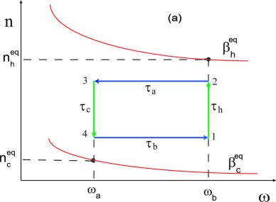
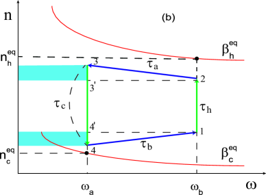
Figure 1: (Color online) Schematic diagram of a quantum Otto cycle working with a harmonic system in the $(\omega,n)$ plane. (a): without nonadiabatic dissipation, (b): with nonadiabatic dissipation. $1\rightarrow 2$ and $3\rightarrow 4$ are two isochoric processes, while $2\rightarrow 3$ and $4\rightarrow 1$ are two adiabatic processes. ${n}_{h}^{eq}$ and ${n}_{c}^{eq}$ are two ratios of the atomic system at thermal equilibrium with two heat reservoirs at inverse temperatures $\beta_{h}$ and $\beta_{c}$.

1. Hot isochore 1$\rightarrow$ 2. The magnetic field $\omega$ is kept fixed at constant value of $\omega_{b}$ and no work is done. The working subsystem is in contact with a hot heat reservoir at inverse temperature $\beta_{h}$ during a period $\tau_{h}$, with $\beta_{h}=1/T_{h}$. It follows, using Eq. (10), that the instantaneous heat flow becomes

$$\frac{{\mathchar 22\relax\mkern-12.0mud}Q_{12}}{dt}=\omega_{b}\frac{df(t)}{dt}=\gamma_{h}\left[{f}_{h}^{eq}-f(t)\right]\omega_{b},$$ (11)

where $\gamma_{h}$ denotes the heat conductivity between the working substance and the hot reservoir and $f_{h}^{eq}$ is the population (or polarization) of the harmonic (or spin) system at thermal equilibrium with the hot reservoir.

In view of the boundary conditons that $f(0)={f}_{1}(\omega_{b},\beta_{1})$ and ${f}(\infty)={f}_{h}^{eq}(\omega_{b},\beta_{h})$, the general solution of Eq. (11) can be readily obtained, ${f}(t)={f}_{h}^{eq}+({f}_{1}-f_{h}^{eq})e^{-\gamma_{h}t}$, resulting in the following relation,

$${f}_{2}=f_{h}^{eq}+(f_{1}-{f}_{h}^{eq}).$$ (12)

Then the heat absorbed directly from the system in the isochoric process becomes

$$Q_{h}\equiv Q_{12}=E_{2}-E_{1}=(f_{2}-{f}_{1})\omega_{b}.$$ (13)

2. Adiabatic expansion $2\rightarrow 3$. The system is decoupled from the hot reservoir, changing $\omega$ from $\omega_{b}$ to $\omega_{a}$ during time $\tau_{a}$. Heat caused by the work to overcome the dissipation is developed and the population or polarization is increased from $f_{2}$ to $f_{3}$, though there is no heat exchanged directly between the system and its surroundings. As in the low-dissipation case Esp10 ; Fel00 ; Wan13 , we assume that the increase of population or of polarization in an adiabatic process is inversely proportional to be the time required for completing this process. Then, we have

$$f_{3}=f_{2}+\sigma_{a}/\tau_{a},$$ (14)

where $\sigma_{a}$ denotes the dissipation coefficient for the adiabatic expansion. The work done directly during this process, $W_{23}^{0}$, can be determined according to

$$W_{23}^{0}=\int_{0}^{\tau_{a}}fd\omega=(\omega_{a}-\omega_{b})\left(f_{2}+\frac{\sigma_{a}}{2\tau_{a}}\right),$$ (15)

while the heat generated on this process in the working substance becomes

$$W_{23}^{add}=Q_{23}=\int_{0}^{\tau_{a}}\omega df=\frac{\sigma_{a}(\omega_{a}+\omega_{b})}{2\tau_{a}},$$ (16)

which is the additional work to overcome the nonadiabatic dissipation. That is, the total work done on the adiabatic compression $2\rightarrow 3$, $W_{23}^{add}$, is given by

$$W_{23}=W_{23}^{0}+W_{23}^{add}=(\omega_{a}-\omega_{b})\left(f_{2}+\frac{\sigma_{a}}{2\tau_{a}}\right)+\frac{\sigma_{a}(\omega_{a}+\omega_{b})}{2\tau_{a}}$$ (17)

3. Cold isochore $3\rightarrow 4$. The system becomes coupled to a cold reservoir at inverse temperature $\beta_{c}$ ($>\beta_{h}$) in a time of $\tau_{c}$. In a way similar to that for the step $1\rightarrow 2$, the heat current in this process can be given by

$$\frac{{\mathchar 22\relax\mkern-12.0mud}Q_{34}}{dt}=\omega_{a}\frac{df(t)}{dt}=\gamma_{c}\left[{f}_{c}^{eq}-f(t)\right]\omega_{a},$$ (18)

thereby yielding the following relation,

$${f}_{4}={f}_{c}^{eq}+({f}_{3}-f_{c}^{eq})e^{-\gamma_{c}\tau_{c}}.$$ (19)

Here $\gamma_{c}$ is the heat conductivity between the working substance and the cold reservoir and $n(t)$ should be restricted by the boundary constraints: $n(0)={n}_{2}(\omega_{a},\beta_{3})$ and ${n}(\infty)={n}_{c}^{eq}(\omega_{a},\beta_{c})$. The amount of heat absorbed by the system from the cold reservoir can be directly calculated as,

$$Q_{c}\equiv Q_{34}=\left|\int_{0}^{\tau_{b}}\omega_{a}df\right|=\omega_{a}\left[(f_{2}-f_{1})+\frac{\sigma_{a}}{\tau_{a}}+\frac{\sigma_{b}}{\tau_{b}}\right].\\$$ (20)

4. Adiabatic compression $4\rightarrow 1$. The frequency $\omega$ is changed from $\omega_{b}$ to its initial value $\omega_{a}$ after time $\tau_{b}$, while $f$ increase from $f_{4}$ to $f_{1}$. The time required for completing this adiabat is $\tau_{b}$. As in the adiabatic expansion $1\rightarrow 2$, we assume

$$f_{1}=f_{4}+\frac{\sigma_{b}}{\tau_{b}},$$ (21)

with $\sigma_{b}$ the dissipation coefficient for the process. It follows, using the computation similar to that for the adiabatic expansion, that the work done and the heat generated on this adiabat are,

$$W_{41}^{0}=\int_{0}^{\tau_{b}}fd\omega=(\omega_{b}-\omega_{a})\left(f_{1}-\frac{\sigma_{b}}{2\tau_{b}}\right),$$ (22)

$$W_{41}^{add}=Q_{41}=\frac{\sigma_{b}(\omega_{a}+\omega_{b})}{2\tau_{b}},$$ (23)

respectively. Then the total work done on this process is,

$$W_{41}=W_{41}^{0}+W_{41}^{add}=(\omega_{b}-\omega_{a})\left(f_{1}-\frac{\sigma_{b}}{2\tau_{b}}\right)+\frac{\sigma_{b}(\omega_{a}+\omega_{b})}{2\tau_{b}}$$ (24)

Repeatedly performing the above sequence of consecutive steps leads to the result that, some of heat systematically extracted from the hot reservoir is released to the cold reservoir, while the rest of the heat is delivered as work. After a single cycle, the total energy of the system as a state function remains unchanged, namely, $\Delta E=Q_{h}-Q_{c}+W_{23}+W_{41}=0$. The total work done by the system per cycle, with $W=-(W_{23}+W_{41})$, and the efficiency are, respectively, given by

$$W_{cylce}=({f}_{2}-{f}_{1})(\omega_{b}-\omega_{a})-\omega_{a}\left(\frac{\sigma_{a}}{\tau_{a}}+\frac{\sigma_{b}}{\tau_{b}}\right),$$ (25)

$$\eta=\frac{W}{Q_{h}}=1-\frac{\omega_{a}}{\omega_{b}}-\frac{\omega_{a}}{\omega_{b}}\frac{\left({\sigma_{a}}/{\tau_{a}}+{\sigma_{b}}/{\tau_{b}}\right)}{(f_{2}-f_{1})}.$$ (26)

On the right hand side of Eq. (25), the first term represents the total positive work done by the system, while the second term is the total negative work done by the system [indicated by the two blue areas in Fig. 1(b)] to overcome internal friction in two adiabats. Eq. (26) shows that the efficiency $\eta$ monotonously decreases as the nonadiabatic dissipation coefficient $\sigma_{a,b}$ increases. For the remainder of the paper, our analysis mainly focuses on the case that the nonadiabatic dissipation is very weak and even vanishing, while the time required for completing the quantum adiabatic process is quite long in order for the quantum adiabatic condition to be satisfied.

IV the efficiency at maximum power output

Following the same approach as in Fel00 , we can derive the following relations by combing Eq. (19) with Eq. (12), ${f}_{2}-{f}_{1}=g(\tau_{c},\tau_{h})\Delta{f}^{eq},$ where

$$g(\tau_{c},\tau_{h})=\frac{(e^{\gamma_{c}\tau_{c}}-1)(e^{\gamma_{h}\tau_{h}}-1)}{e^{\gamma_{c}\tau_{c}+\gamma_{h}\tau_{h}}-1}$$ (27)

and $\Delta{n}^{eq}={n}_{h}^{eq}-{n}_{c}^{eq}$, with $\Delta{f}^{eq}=f(e^{-\beta_{c}\omega_{a}})-f(e^{-\beta_{h}\omega_{b}}).$

Considering $\tau_{cycle}=\tau_{c}+\tau_{h}+\tau_{adi}$, with $\tau_{adi}\equiv\tau_{a}+\tau_{b}$ the total time required for completing the two adiabatic processes, and using Eq. (25), we can derive the power output as,

$$P=\frac{W}{\tau_{cycle}}=\frac{1}{\tau_{cycle}}\left[(\omega_{b}-\omega_{a})\Delta{f}^{eq}g(\tau_{c},\tau_{h})-\omega_{a}\left(\frac{\sigma_{a}}{\tau_{a}}+\frac{\sigma_{b}}{\tau_{b}}\right)\right].$$ (28)

We find that, from Eq. (28), the positive work condition is

$$\Delta f^{eq}>\frac{\omega_{a}}{(\omega_{b}-\omega_{a})}\frac{(\sigma_{a}/\tau_{a}+\sigma_{b}/\tau_{b})}{g(\tau_{c},\tau_{h})},$$ (29)

which must be satisfied in order that our engine model can produce positive work. In the ideal case when the adiabatic process is isentropic and thus $\sigma_{a}=\sigma_{b}=0$, the power output in Eq. (28) and the positive work condition in Eq. (29) then simplify to

$$P=\frac{g(\tau_{c},\tau_{h})}{\tau_{cycle}}(\omega_{b}-\omega_{a})\Delta{f}^{eq},$$ (30)

$$\frac{\omega_{b}}{\omega_{a}}<\frac{\beta_{c}}{\beta_{h}}=\frac{T_{h}}{T_{c}},$$ (31)

respectively. Note that, the positive condition (31) confirms the Carnot’s theorem.

It can be seen from Eq. (26) that, the efficiency increases monotonously with decrease in the dissipation coefficients $\sigma_{a,b}$ and approaches the upper bound, $\eta_{+}$, when $\sigma_{a,b}$ are vanishing. Now let us consider the upper bound of the EMP, which is obtained in the heat engine with two isentropic processes, within the assumption that the time allocations to the two isochores ($\tau_{c}$ and $\tau_{h}$) and to the adiabats $\tau_{adi}$ are given. Based on Eq. (A.11), optimizing power output becomes equivalent to optimizing two values of external fields $\omega_{a}$ and $\omega_{b}$. In the Appendix, we show that, setting $\partial{P}/\partial{\omega_{a}}=0$ and $\partial{P}/\partial{\omega_{b}}=0$, the EMP can be approximated analytically by,

$$\eta_{mp}=\frac{\eta_{C}^{2}}{\eta_{C}-(1-\eta_{C})\ln({1-\eta_{C}})},$$ (32)

whether for a spin-$1/2$ or for a harmonic system. This expression of EMP, as one main result of the present paper, was previously obtained for the heat engine based on a two-level atomic system Wan13 , Feynman’s ratchet Tuz08 , or the classical transport Van12 . We have proved in Appendix that the EMP given by Eq. (32) holds well in the region of all finite temperatures, neither restricted to the classical limit when the temperatures high enough nor to the linear-response regime when $\Delta(1/\beta)\rightarrow 0$ with $\Delta(1/\beta)=1/\beta_{h}-1/\beta_{c}$. It is interesting to note that, in contrast to the classical Otto engine where the EMP is dependent on the working substance Guo13 , the QOEs based on a spin or a harmonic system have the same upper bound of the EMP, which is attainable as nonadiabatic dissipation is vanishing.

Expanding $\eta_{+}$ up to the third term of $\eta_{C}$ gives rise to $\eta_{mp}=\eta_{C}/2+\eta_{C}^{2}/8+7\eta_{C}^{3}/96+O(\eta_{C}^{4})$, which is in nice agreement with the expansion of the CA efficiency $\eta_{CA}$, with $\eta_{CA}=\eta_{C}/2+\eta_{C}^{2}/8+16\eta_{C}^{3}/96+O(\eta_{C}^{4})$. The values of EMP $\eta_{+}$ derived here are very close to those of the $CA$ efficiency $\eta_{CA}$, particularly at small relative difference temperatures they have the same universality, ${\eta_{C}}/2+{\eta_{C}^{2}}/8$.

V Irreversible thermodynamics

We consider the Onsager relations and the EMP by mapping our model into a general linear irreversible heat engine, when the model proceeds in the linear-response regime. We assume that the heat engine is working in the linear-response regime where the temperature difference $\Delta T=T_{h}-T_{C}$ is very small. The work is performed under an external force $F$ and it is determined by $W=Fx$, where $x$ is the thermodynamically conjugate variable of $F$. In the linear-response regime with $\Delta T\rightarrow 0$, a thermodynamic force $X_{1}=F/T_{c}\simeq F/T,$ where $T\equiv(T_{c}+T_{h})/2$ and its conjugate flux $J_{1}=\dot{x}$. We also define the inverse temperature difference $1/T_{c}-1/T_{h}\simeq\Delta T/T^{2}$ as another thermodynamic force $X_{2}$ and the heat flux $\dot{Q}_{h}$ as its conjugate flux $J_{2}$.

The Onsager relations are used to describe these fluxes and forces as:

$$J_{1}=L_{11}X_{1}+L_{12}X_{2},$$ (33)

$$J_{2}=L_{21}X_{1}+L_{22}X_{2},$$ (34)

where $L_{ij}$’s are the Onsager coefficients with the symmetry relation $L_{12}=L_{21}$. Since the entropy variation of working substance which comes back to its original state is vanishing for our engine model after a whole cycle, the entropy production rate $\dot{\sigma}$ can be expressed as $\dot{\sigma}=-\frac{\dot{Q}_{h}}{T_{h}}+\frac{\dot{Q}_{c}}{T_{c}}=-\frac{\dot{W}}{T_{h}}+{\dot{Q}_{c}}({\frac{1}{T_{c}}-\frac{1}{T_{h}}}),$ where the dot denotes a quantity quantity divided by the cycle period $\tau_{cycle}$. In the linear response regime where $\Delta T\rightarrow 0$, $\dot{\sigma}$ can be approximated by

$$\dot{\sigma}\simeq-\frac{{W}}{T}\frac{1}{\tau_{cycle}}+{\dot{Q}_{c}}\frac{\Delta T}{T^{2}},$$ (35)

where the higher terms like $O(\Delta T\dot{W})$ and $O(\Delta T^{3}\dot{Q}_{c})$ have been neglected. Considering the decomposition $\dot{\sigma}=J_{1}X_{1}+J_{2}X_{2}$, we can define the thermodynamic Izu09 ; Izu10 ; Shen14 . force as

$$X_{1}=-\dot{W}/{T},X_{2}={\Delta T}/{T^{2}},$$ (36)

and their conjugate thermodynamic forces

$$J_{1}=1/{\tau_{cycle}},J_{2}=\dot{Q}_{c}.$$ (37)

Considering the Carnot’s theorem, we have $\eta=1-{\omega_{a}}/{\omega_{b}}\leq\eta_{C}=1-{T_{c}}/{T_{h}}$, and in the linear response regime

$$\Delta\omega/\omega\leq{\Delta T}/{T}.$$ (38)

Here and hereafter we use $\Delta\omega=\omega_{b}-\omega_{a}$ with $\omega\equiv(\omega_{a}+\omega_{b})/2$. When the QOE works in the linear response regime $\Delta T\rightarrow 0$ but it can still produce positive work, even the Carnot efficiency $\eta_{C}\simeq{\Delta T}/{T}$ (as the upper bound of the efficiency $\eta$) tends to be vanishing, implying that we may assume $\Delta\omega/\omega\simeq\Delta T/T\rightarrow 0$.

We turn to the explicit calculation of the Onsager coefficients $L_{ij}$’s, adopting an approach similar to ones used in theoretical models of a Brownian and a macroscopic Carnot cycle Izu09 ; Izu10 . To determine $L_{11}$, we consider the relation between $1/{\tau_{cycle}}$ and $X_{1}$ in the case of $\Delta T\rightarrow 0$ as well as $\Delta\omega\rightarrow 0$. For simplicity, we assume $\sigma_{a}\equiv\sigma_{b}\equiv\sigma/4$, $\tau_{a}\equiv\tau_{b}\equiv\tau_{cycle}/\alpha$ with $\alpha>1$ in the following. From Eq. (20), then the amount of heat released to the cold reservoir becomes

$$Q_{c}=\omega_{a}\Delta f^{eq}g-\frac{\omega_{a}\sigma\alpha}{\tau_{cycle}}.$$ (39)

Since $\Delta T\rightarrow 0$, from Eq. (28) we can write using $\Delta\omega\rightarrow 0$ the work $W$ as

$$W=\Delta\omega\Delta f^{eq}g-\frac{\omega_{a}\sigma\alpha}{\tau_{cycle}}.$$ (40)

Setting $\Delta\omega=\Delta T=0$ in Eq. (40), we have by using the approximation $\omega_{a}\simeq\omega_{b}\simeq\omega$,

$$\frac{1}{\tau_{cycle}}=\frac{T}{\omega\alpha\sigma}\frac{-W}{T},$$ (41)

which, together with Eqs. (33) and (36), gives rise to

$$L_{11}=\frac{T}{\omega\sigma\alpha}.$$ (42)

Likewise $\dot{Q}_{c}$ at $\Delta T=0$ can be expressed by using Eqs. (39) and (41)as

$$\dot{Q}_{c}=\frac{Tg{\Delta f^{eq}}}{\alpha\sigma}\frac{-W}{T}-\frac{\omega\sigma\alpha}{\tau_{cycle}^{2}}.$$ (43)

Since the second term in the above equation is $O(W^{2})$ quantity from Eq. (41), $\dot{Q}_{c}$ with $\Delta T=0$ can be evaluated up to the linear order of $W$,

$$\dot{Q}_{c}=\frac{Tg{\Delta f^{eq}}}{\alpha\sigma}\frac{-W}{T}.$$ (44)

From Eqs. (34) and (36), the coefficient $L_{21}$ is determined according to

$$L_{21}=\frac{Tg{\Delta f^{eq}}}{\alpha\sigma}.$$ (45)

Here $g=g(\tau_{c},\tau_{h})$ defined above Eq. (27) is a function of the time $\tau_{c}$ and $\tau_{h}$, and it is thus a function of the cycle time $\tau_{cycle}$(=$1/J_{1})$. However, the value of parameter $g$, situated between $0\leq g\leq 1$, is dimensionless and it can then be casted into the expressions of the Onsager coefficients.

In the linear-response regime when $\Delta T\rightarrow 0$, we can assume from Eq. (38) that $\Delta\omega/\omega\simeq\Delta T/T\rightarrow 0$; therefore $W$ in Eq. (40) is approximately

$$W={T\omega\Delta f^{eq}g}\frac{\Delta T}{T^{2}}-\frac{\omega\sigma\alpha}{\tau_{cycle}}.$$ (46)

When setting $W=0$, we can obtain from Eq. (46),

$$\frac{1}{\tau_{cycle}}=\frac{Tg{\Delta f^{eq}}}{\sigma\alpha}\frac{\Delta T}{T^{2}}.$$ (47)

Substitution of $W=0$ into Eq. (40) leads to

$$L_{12}=\frac{Tg{\Delta f^{eq}}}{\sigma\alpha}.$$ (48)

From Eqs. (45) and (48), we see that the Onsager symmetry relation $L_{21}=L_{12}$ is confirmed as expected. In the case of $W=0$, $\dot{Q}_{c}$ can be derived from Eqs. (39) and (47) as

$$\dot{Q}_{c}=\frac{\omega T(\Delta f^{eq})^{2}g^{2}}{\sigma\alpha}\frac{\Delta T}{T^{2}}-\frac{\omega\sigma\alpha}{\tau_{cycle}^{2}}.$$ (49)

Since here the second term is $O(\Delta T^{2})$ quantity, we can neglect this term and then obtain

$$L_{22}=\frac{\omega T(\Delta f^{eq})^{2}g^{2}}{\sigma\alpha}.$$ (50)

As expected, these Onsager coefficients derived in our model satisfy the constraints $L_{11}\geq 0,L_{22}\geq 0$ and $L_{11}L_{22}-L_{12}L_{21}\geq 0$, which originates from the positivity of the entropy production rate $\dot{\sigma}$.

Now consider EMP for our linear irreversible heat engine, following the approach first proposed in Van05 . With consideration of Eqs. (36) and (37), the power and the efficiency can be expressed as $P=\dot{W}=-J_{1}X_{1}T$, and $\eta={\dot{Q}_{h}}/{\dot{W}}=-{J_{2}}/{(J_{1}X_{1}T)}$, respectively. It then follows, using the condition ${\partial P}/{\partial X_{1}}=0$, that the EMP takes the form as $\eta^{*}=\frac{\Delta T}{2T}\frac{q^{2}}{1-q^{2}}$, where $q=L_{12}/\sqrt{L_{11}L_{22}}$ as the coupling strength parameter has been used. These Onsager coefficients given by Eqs. (42), (45), (48), and (50) show that here the linear irreversible heat engine satisfies the tight-coupling condition $|q|=1$. In such case, the EMP becomes Izu10

$$\eta_{mp}=\frac{\Delta T}{2T}=\eta_{CA}+O(\Delta T^{2}).$$ (51)

It is also the upper bound of EMP since the coupling strength parameter satisfies the relation $|q|\leq 1$ which is equivalent to the condition that $L_{11}\geq 0,L_{22}\geq 0$ and $L_{11}L_{22}-L_{12}L_{21}\geq 0$.

VI Conclusions

We have employed both finite-time and irreversible thermodynamics to consider the EMP for a QOE, in which the working substance is composed of a spin-$1/2$ and a harmonic system. From a view point of finite-time thermodynamics, we showed that the EMP, wether for the spin or harmonic system, is bounded from above the same value $\eta_{+}$ determined by Eq. (1) which displays the same universality as $\eta_{CA}$ at small relative temperature differences. Within the framework of the linear irreversible thermodynamics, we proved that $\eta_{CA}$ is the upper bound of the EMP for the heat engines in linear response regime when the temperature difference $\Delta T\rightarrow 0$, and we also calculated the Onsager coefficients for the irreversible QOEs.

Acknowledgements

This work is supported by the National Natural Science Foundation of China under Grants No. 11265010, No. 11375045, and No. 11365015; the State Key Programs of China under Grant No. 2012CB921604; and the Jiangxi Provincial Natural Science Foundation under Grant No. 20132BAB212009, China.

Appendix A Analytical expression of EMP for a QOE working with a harmonic or a spin-$1/2$ system

A.1 For a harmonic system

In the case when the working substance is a harmonic system, the power output becomes

$$P=\frac{W}{\tau_{cycle}}=\frac{1}{2}G(\tau_{c},\tau_{h})(\omega_{b}-\omega_{a})[\coth{(\beta_{h}\omega_{b})}-\coth{(\beta_{c}\omega_{a})}].$$ (A.1)

Then, the extremal conditions of ${\partial P}/{\partial\omega_{a}}=0$ and ${\partial P}/{\partial\omega_{b}}=0$ lead to

$$(\omega_{b}-\omega_{a})\beta_{c}=\left[\coth\left(\frac{\omega_{a}\beta_{c}}{2}\right)-\coth\left(\frac{\omega_{b}\beta_{h}}{2}\right)\right]\sinh^{2}\left(\frac{\omega_{a}\beta_{c}}{2}\right),$$ (A.2)

$$(\omega_{b}-\omega_{a})\beta_{h}=\left[\coth\left(\frac{\omega_{a}\beta_{c}}{2}\right)-\coth\left(\frac{\omega_{b}\beta_{h}}{2}\right)\right]\sinh^{2}\left(\frac{\omega_{b}\beta_{h}}{2}\right).$$ (A.3)

Dividing directly both sides of Eq. (A.2) by Eq. (A.3) and defining $r=\sqrt{\beta_{c}/\beta_{h}}$, we have

$$\frac{1}{r}=\frac{{1/x_{h}}-x_{h}}{{1/x_{c}}-x_{c}},$$ (A.4)

in which $x_{h}\equiv e^{-\frac{\omega_{b}\beta_{h}}{2}}$ and $x_{c}\equiv e^{-\frac{\omega_{a}\beta_{c}}{2}}$. The physical solution to Eq. (A.4) can be obtained,

$$x_{h}=\frac{\sqrt{x_{c}^{4}+(4r^{2}-2)x_{c}^{2}+1}+x_{c}^{2}-1}{2rx_{c}},$$ (A.5)

from which we expand $x_{h}$ up to the sixth order:

$$x_{h}=rx_{c}-r(r^{2}-1)x_{c}^{3}+r(r^{2}-1)(2r^{2}-1)x_{c}^{5}+O(x_{c}^{7}).$$ (A.6)

From Eq. (A.5), we note that the condition $x_{c}^{2}-(4r^{2}-2)x_{c}+1>0$ must be satisfied in order for $x_{h}$ to be a real number. This condition, together with the fact that $0<x_{c}<1$, leads to $0<x_{c}\leq x_{c}^{+}$, where $x_{c}^{+}=-\sqrt{(2r^{2}-1)^{2}-1}+2r^{2}-1$ is the upper bound of $x_{c}$. Here $x_{c}^{+}$ is the same as corresponding one derived from the two-level atomic system [see Appendix in Ref. Rui13]. We can think of two effective facts: (1) the upper bound of $x_{c}$ decreases quickly with increasing $r$ and rapidly approaches zero, favoring $x_{h}\simeq rx_{c}$ when $r\gg 1$ and $x_{c}^{+}\rightarrow 0$; and (2) if $r$ is approximated equal to $1$, the expansion coefficients on the right side of Eq. (A.6) becomes vanishing, favoring $x_{h}\simeq rx_{c}$ when $r\rightarrow 1$ and $x_{c}^{+}\rightarrow 1$. That is, Eq. (A.6) can be simplified as

$$x_{h}=rx_{c}.$$ (A.7)

This approximation is valid, but not restricted to the linear-response regime $\Delta{1/\beta}\rightarrow 0$ with $\Delta{(1/\beta)}=1/\beta_{h}-1/\beta_{c}$ (i.e., $r\rightarrow 1$) or to the high-temperature limit when $\beta\omega\ll 1$ (i.e., $x_{c}\rightarrow 1$).

When we multiply both sides of Eqs. (A.2) and (A.3), we obtain $\omega_{b}-\omega_{a}=(2\sinh(\omega_{a}\beta_{c}-\omega_{b}\beta_{h})/\sqrt{\beta_{c}\beta_{h}}$, or

$$2\left(\frac{\ln x_{c}}{\beta_{c}}-\frac{\ln x_{h}}{\beta_{h}}\right)=\frac{x_{h}/x_{c}-x_{c}/x_{h}}{\sqrt{\beta_{c}\beta_{h}}},$$ (A.8)

where $x_{c}$ and $x_{h}$ were defined in Eq. (A.4). Considering Eqs. (A.7) and (A.8), we have

$$\ln{x_{c}}=\frac{(r^{2}-1)\sqrt{\beta_{c}\beta_{h}}+2r\beta_{c}\ln(r)}{2r(\beta_{h}-\beta_{c})},$$ (A.9)

and

$$\ln{x_{h}}=\ln x_{c}+\ln r.$$ (A.10)

Substituting $r=1/\sqrt{1-\eta_{c}}$, with the Carnot efficiency $\eta_{c}=1-\beta_{h}/\beta_{c}$, into the expression $\eta^{*}=1-\frac{\omega_{a}}{\omega_{b}}=1-\frac{\beta_{h}\ln{x_{c}}}{\beta_{c}\ln{x_{h}}}$, we then derive the analytical expression of EMP [see Eq. (32)].

A.2 For a spin$-1/2$ system

If the working substance is a spin$-1/2$ system, then the power output for the heat engine becomes

$$P=\frac{W}{\tau_{cycle}}=\frac{1}{2}G(\tau_{c},\tau_{h})(\omega_{b}-\omega_{a})[\tanh{(\beta_{c}\omega_{a})}-\tanh{(\beta_{h}\omega_{b})}].$$ (A.11)

We set ${\partial P}/{\partial\omega_{a}}=0$ and ${\partial P}/{\partial\omega_{b}}=0$, obtaining

$$(\omega_{b}-\omega_{a})\beta_{c}=\left[\tanh\left(\frac{\omega_{a}\beta_{c}}{2}\right)-\tanh\left(\frac{\omega_{b}\beta_{h}}{2}\right)\right]\cosh^{2}\left(\frac{\omega_{a}\beta_{c}}{2}\right),$$ (A.12)

$$(\omega_{b}-\omega_{a})\beta_{h}=\left[\tanh\left(\frac{\omega_{a}\beta_{c}}{2}\right)-\tanh\left(\frac{\omega_{b}\beta_{h}}{2}\right)\right]\cosh^{2}\left(\frac{\omega_{b}\beta_{h}}{2}\right).$$ (A.13)

Based on Eqs. (A.12) and (A.13), we find, in the same way that we derived Eqs. (A.5) and (A.9), and that for the spin$-1/2$ system, optimal relations among $x_{c},x_{h}$ and $r$ are also determined by Eqs. (A.5) and (A.9), and (A.10). As a consequence, the EMP for a heat engine working with a spin$-1/2$ system can be approximated by Eq. (32), the same as one obtained from the heat engine based on the harmonic system.

(A.14)

References

• (1) F. Curzon and B. Ahlborn , Am. J. Phys. 43, 22 (1975).
• (2) M. Esposito, R. Kawai, K. Lindenberg, and C. Van denBroeck, Phys. Rev. Lett. 105, 150603 (2010).
• (3) B. Gaveau, M. Moreau, and L. S. Schulman, Phys. Rev. Lett. 105, 060601 (2010).
• (4) U. Seifert, Phys. Rev. Lett. 106, 020601 (2011).
• (5) T. Schmiedl and U. Seifert, Europhys. Lett. 81, 20003 (2008).
• (6) A. Gomez-Marin, J.M. Sancho, Phys. Rev. E 74, 062102(2006)
• (7) Y. Wang and Z. C. Tu, Phys. Rev. E 85, 011127 (2012); Europhys. Lett. 98, 40001 (2012).
• (8) C. Van den Broeck and K. Lindenberg, Phys. Rev. E 86, 041144 (2012).
• (9) J. Guo, J. Wang, Y. Wang, and J. Chen, Phys. Rev. E 87, 012133 (2013).
• (10) S. Sheng and Z. C. Tu, Phys. Rev. E 89, 012129 (2014).
• (11) A. E. Allahverdyan, K. V. Hovhannisyan, A. V. Melkikh, and S. G. Gevorkian, Phys. Rev. Lett. 111, 050601 (2013).
• (12) B. Jiménez de Cisneros, A. Calvo Hernández, Phys. Rev. Lett. 98, 130602 (2007)
• (13) R. Wang, J. H. Wang, J. Z. He, and Y. L. Ma, Phys. Rev. E 87, 042119 (2013).
• (14) Z. C. Tu, J. Phys. A: Math. Theor. 41, 312003 (2008).
• (15) A. E. Allahverdyan, R. S. Johal, G. Mahler, Phys. Rev. E 77, 041118 (2008)
• (16) R. Kosloff, Entropy 15, 2100 (2013).
• (17) R. Kosloff and A. Levy, Annu. Rev. Phys. Chem. 65, 365 (2014).
• (18) J. H. Wang, J. Z. He, and Z. Q. Wu, Phys. Rev. E 85, 031145 (2012).
• (19) F.Wu, L. G. Chen, S.Wu, F. R. Sun, and C.Wu, J. Chem. Phys. 124, 214702 (2006); J. Appl. Phys. 99, 054904 (2006). X. L.
• (20) Y. Rezek and R. Kosloff, New J. Phys. 8, 83 (2006).
• (21) X. L. Huang, T. Wang, and X. X Yi, Phys. Rev. E 86, 051105 (2012).
• (22) J. H. Wang, Z. Q. Wu, and J. Z. He, Phys. Rev. E 85, 041148 (2012).
• (23) T. Feldmann and R. Kosloff, Phys. Rev. E 61, 4774 (2000).
• (24) Huang, L. C. Wang, and X. X. Yi, Phys. Rev. E 87, 012144 (2013).
• (25) O. Abah, J. Roßagel, G. Jacob, S. Deffner, F. Schmidt-Kaler, K. Singer, and E. Lutz, Phys. Rev. Lett. 109, 203006 (2012).
• (26) C. Van den Broeck, Phys. Rev. Lett. 95, 190602 (2005).
• (27) C. Van den Broeck, R. Kawai, P. Meurs, Phys. Rev. Lett. 93, 090601 (2004)
• (28) C. Van den Broeck, R. Kawai , Phys. Rev. Lett. 96, 210601 (2006)
• (29) Y. Izumida and K. Okuda, Eur. Phys. J. B 77, 499(2010).
• (30) B. Rutten, M. Esposito, and B. Cleuren, Phys. Rev. B 80, 235122 (2009); B. Cleuren, B. Rutten, and C. Van den Broeck, Phys. Rev. Lett. 108, 120603 (2012).
• (31) Y. Izumida, K. Okuda, Phys. Rev. E 80, 021121 (2009).
• (32) Y. Apertet, H. Ouerdane, C. Goupil, and Ph. Lecoeur, Phys. Rev. E 85, 041144 (2012).
• (33) B. Andresen, P. Salamon, and R. S. Berry, Phys. Today 37(9), 62 (1984).
• (34) B. Andresen, R. S. Berry, A. Nitzan, and P. Salamon,Phys. Rev. A 15, 2086 (1977).
• (35) Z. Yan and J. Chen, J. Phys. D: Appl. Phys. 23, 136(1990).
• (36) L. Chen, C. Wu, and F. Sun, J. Non-Equilib. Thermodyn. 24(4), 327 (1999).
• (37) Y. Izumida and K. Okuda, Phys. Rev. E 80, 021121 (2009).
• (38) Y. Izumida and K. Okuda, Europhys. Lett. 97, 10004 (2012).
• (39) Y. Izumida, K. Okuda, A. Calvo Hernández, and J. M. M. Roco, Europhys. Lett. 101, 10005 (2013).
• (40) E. Geva and R. Kosloff, J. Chem. Phys. 96, 3054 (1992); J. Chem. Phys. 97, 4398, (1992).
• (41) M. Born and V. Fock, Z. Phys. 51, 165 (1928).