The nonperturbative structure of hadrons

Abstract

In this thesis we explore a diverse array of issues that strike at the inherently nonperturbative structure of hadrons at momenta below the QCD confinement scale. In so doing, we mainly seek a better control over the partonic substructure of strongly-interacting matter, especially as this relates to the nonperturbative effects that both motivate and complicate experiments — particularly DIS; among others, such considerations entail sub-leading corrections in $Q^{2}$, dynamical higher twist effects, and hadron mass corrections. We also present novel calculations of several examples of flavor symmetry violation, which also originates in the long-distance properties of QCD at low energy. Moreover, we outline a recently developed model, framed as a hadronic effective theory amenable to QCD global analysis, which provides new insights into the possibility of nonperturbative heavy quarks in the nucleon. This model can be extended to the scale of the lighter mesons, and we assess the accessibility of the structure function of the interacting pion in the resulting framework.

J. T. Londergan, Ph.D.              W. Melnitchouk, Ph.D.              L. Kaufman, Ph.D.

J. Liao, Ph.D.                          W. M. Snow, Ph.D.

Chapter 0 Introduction

“If I were again beginning my studies, I would follow the advice of Plato and start with mathematics.”
      — Galileo Galilei

In what was arguably the most startling intellectual development of human scientific history, the early 20^th Century heralded the final unification of Planckian Quantum Mechanics and Einsteinian relativity. Since then, rapid progress has been made in directing the resulting synthesis – Quantum Field Theory (QFT) – toward a total description of microscopic matter.

Though unquestionably novel, the insights that bequeathed QFT belong to the same historical tradition that in the West originated with the Milesian materialists Thales and Anaximander, as well as the early atomists of Abdura, among whom the great Democritus [3] is likely the best known today.

Sadly, this enlightened perspective languished in relative obscurity for millenia, not again being embraced until the chemical analyses of Dalton [4] and Lavoisier; even then, the reality and nature of the atomic hypothesis remained controversial up to the time of J. J. Thomson’s discovery of the electron [5] in 1897, and the complementary discovery of the atomic nucleus [6] by Rutherford, Geiger, and Marsden in 1909. With these confirmations as well as observations of the emission spectra of hydrogen, Bohr’s universally recognizable planetary model quickly followed, absorbing several modifications in response to the wave formalism of Schrödinger.

The disunity of special relativity and quantum mechanics was a preventative roadblock to a theory of (sub-)atomic interactions with electromagnetic fields until the QFT of Dirac [7], Fermi and others was shown to be renormalizable by Bethe; the resulting $U(1)$ theory of QED was especially facile in describing spectral line shifts of electromagnetic bound states (e.g., the Lamb shift in hydrogen), as well as the outcomes of various scattering experiments — $e^{-}e^{-}$ M$\o$ller reactions, the Bhahba process $e^{-}e^{+}$, and electron-muon interactions.

On the other hand, the remarkably short lifetimes involved in nuclear decays indicated that an enormously stronger force was required to bind a nucleus of net positive electric charge. For this reason, despite successes describing the electromagnetic interaction, initial doubts regarding the general applicability of field-theoretic methods to the dynamics of strongly bound matter led to early attempts based on $S$-matrix theory; among these were Regge theory [8] and the ‘bootstrap’ scheme [9] of Chew. Now largely defunct, the latter of these envisioned a “nuclear democracy” of hadronic states, each nested within the other, thereby leading to a situation in which there simply were no fundamental states. Among its advocates, the bootstrap paradigm was thought to constrain the S-matrix under the auspices of unitarity, analyticity, and crossing symmetries, but additionally required a ‘narrow resonance’ approximation to produce scattering amplitudes with mixed success.

As an alternative, Regge theory endeavored to describe amplitudes in strong interaction physics as arising from exchanges of states of specific angular momentum, themselves belonging to a complex space of linear ‘trajectories’ $\alpha_{J}(t)$. This framework leads to a simple prediction for the $(s,\ t)$ dependence of hadronic scattering amplitudes:

$$A(s,\ t)\ \sim\ e^{\alpha_{J}(t)\ \cdot\ \ln(s/s_{0})}\ .$$ (1)

Perhaps ironically, Regge theory remains among the more competitive tools in ongoing efforts to unite the unresolved details of short- vs. long-distance physics in QCD as we shall briefly describe in Chap. 1.2.

Figure 1: (Left) The flavor $SU(3)$ octet of spin-1/2 baryons. (Right) The corresponding pseudoscalar meson nonet.

The doubts in more field-theoretic approaches were partially driven by the physical logic embodied in observations by Landau [10] that charge screening phenomena connected to the perturbative calculability of QED had no clear analogue in the physics of hadrons. While these quandaries stymied theoretical efforts, advances at the early generation of colliders at Stanford and other experimental facilities revealed an increasingly rich landscape of mesons and baryons, leading Gell-Mann [11] and Zweig [12] to the natural suspicion that this proliferation in the hadronic spectrum was evidence of an underlying flavor symmetry generated by the constituent degrees of freedom – called ‘quarks’ by Gell-Mann. (Zweig’s alternative moniker ‘aces’ never quite caught on.) Hence the now-famous eight-fold way deduced with Ne’eman presents the lightest spin-$1/2$ baryons as belonging to a flavor octet generated by an approximate $SU(3)$ flavor symmetry, whereas the higher spin resonances form a decuplet. Similar flavor multiplets were found to hold for the pseudoscalar and vector meson nonets. For the sake of illustration, the $SU(3)$ spin-$1/2$ baryons and pseudoscalar mesons are ordered in typical fashion according to charge and strangeness in the left and right panels of Fig. 1.

Contemporaneously, the fact that the nucleon was not fundamental and possessed some non-trivial distribution of electric and magnetic charge was made clear by the characteristic decrease with $Q^{2}$ of the electromagnetic form factors $G_{E}(Q^{2}),\,G_{M}(Q^{2})$ measured in the pioneering elastic electron-proton experiments conducted by Hofstadter et al. [13, 14]. At much the same time, some of the first results from the early generation of electron-nucleon deeply inelastic scattering (DIS) experiments began to emerge; perhaps among the more suggestive results obtained was the unexpected behavior of the cross section ratio for longitudinally vs. transversely polarized photons, namely, that $R=\sigma^{L}/\sigma^{T}\sim 0$ for $Q^{2}\to\infty$ at fixed $x$. For reasons that will be explained in greater detail in Chap. 2, this was a striking affirmation that the sub-nucleonic constituents of the proton were indeed charge-carrying, spin-1/2 fermions.

All the more, these measurements also presented the first direct experimental confrontation with Bjorken’s current algebra scheme. In another attempt at side-stepping the problems known to plague formal field theories of the strong interaction, current algebra suggested that DIS cross sections should depend only upon the single parameter $x$ (rather than the two permitted by kinematical considerations, $(x,\,Q^{2})$, as discussed in Chap. 1.1), in a phenomenon which came to be known as ‘scaling.’ [15]

Physically due to scattering from individual, weakly-interacting partons, scaling was mysterious in the setting of generic, perturbative QFTs, in which resummation of corrections to all orders would presumably lead to divergences and the irresolvable breaking of scaling. However, the properties of non-Abelian field theories, together with the dimensional regularization procedures introduced by ’t Hooft and Veltman [16] in the end provide the answer. Such a Yang-Mills theory can be constructed in terms of quarks, with gauge invariance specifying the interactions. The result is the modern theory of the strong interaction – quantum chromodynamics (QCD).

Formally, the degrees of freedom of QCD are quarks and gluons, and their interactions in the asymptotic limit are governed by a simple lagrangian:

$${\cal L} =\sum_{q}\bar{\psi}_{q,a}(i[\not{\partial}+im_{q}]\delta_{ab})-\alpha_{s}\gamma^{\mu}t_{ab}^{C}A_{\mu}^{C})\psi_{q}^{b}-\frac{1}{4}\mathcal{G}^{i}_{\mu\nu}\mathcal{G}^{i\ \mu\nu}$$

$$\mathcal{G}^{i}_{\mu\nu} =\partial_{\mu}A^{i}_{\nu}-\partial_{\nu}A^{i}_{\mu}-\alpha_{s}f_{ijk}A^{j}_{\mu}A^{k}_{\nu},$$ (2)

where the QCD $SU(3)$ structure constants are determined from the Gell-Mann algebra by $[t^{i},t^{j}]=if_{ijk}\,t^{k}$.

In the fundamental representation $SU(N)$, the beta function of non-Abelian gauge theory describes the dependence of the renormalized strong coupling $\alpha_{s}$ on the regularization scale $\mu$ to an arbitrary order in perturbation theory. At leading order, the famous result as first isolated from the lagrangian of Eq. (2) by Gross, Wilczek, and Politzer [17] was found to be

$$\beta(\alpha_{s})\ =\ \partial\alpha_{s}\Large/\partial\log\mu$$

$$=\ -\left({11\over 3}\ T_{A}\ -\ {4\over 3}n_{F}\ T_{R}\right)\ {\alpha_{s}^{2}\over 2\pi}\ +\ \mathcal{O}(\alpha_{s}^{3})\ ,$$

$$T_{A}=3,\ \,\,\,T_{R}=1/2\ \implies\ -\left(11\ -\ {2\over 3}n_{F}\right)\ {\alpha_{s}^{2}\over 2\pi}\ +\ \mathcal{O}(\alpha_{s}^{3})\ ,$$ (3)

which is clearly negative for any choice of flavor number $n_{F}\leq 16$. This profound result, possible only in the context of non-Abelian gauge theories, is in fact the finding that unifies the disparate problems just described and renders them solvable.

Figure 2: (Left) The WA25 test [18] of the GLS sum rule defined by Eq. (5a). (Right) The analogous NMC experimental test [19] of the Gottfried sum rule compared with various model predictions of [20]. The data are plotted in bins of a lower integration bound $x$, such that the relation in Eq. (5b) is recovered in the limit $x\rightarrow 0$.

When the predictions of QCD are married to the quark-parton model (QPM) formulated by Feynman with the impulse approximation [21], the basic framework for hadronic phenomenology emerges. Apropos, a crucial confirmation of the basic contours of the QPM came in the form of various sum rules devised with current algebra under the assumption that the partons responsible for Bjorken scaling were in fact the quark-level degrees of freedom of QCD. Actually, there are several such relations, all of which emanate from number conservation arguments applied to the electroweak structure functions to be introduced in detail in Chap. 2.

In particular, the QPM treats the nonperturbative portion of the spin-independent nucleon wavefunction as being dominated by its valence quark content, which is itself represented by the $C$-odd combinations of quark and antiquark distributions $q_{v}(x)=q(x)-\bar{q}(x)$. These distributions are inherently probabilistic and therefore satisfy normalization conditions in the proton (in accordance with the quarks’ fractional charges):

$$\int_{0}^{1}\ dx\ u_{v}(x,Q^{2})\ =\ 2\ ,\,\,\,\,\,\,\,\int_{0}^{1}\ dx\ d_{v}(x,Q^{2})\ =\ 1\ .$$ (4)

Of course these quantities reside in the structure functions moments, and impose certain behaviors that may be readily derived; of especial relevance to this thesis are the weak interaction Gross-Llewellyn-Smith (GLS) and Gottfried sum rules, which we list up to first-order corrections in $\alpha_{s}$ as

$$(\mathrm{GLS})\ \,\,\,\,\, \rightarrow\ \,\,\,\,\,{1\over 2}\ \int_{0}^{1}\ dx\ \Big{(}F^{W^{-}}_{3}(x,Q^{2})+F^{W^{+}}_{3}(x,Q^{2})\Big{)}\ =\ 3\ ,$$ (5a)

$$(\mathrm{Gottfried})\ \,\,\,\,\, \rightarrow\ \,\,\,\,\,\,\,\,\,\,\int_{0}^{1}\ {dx\over x}\ \Big{(}F^{p}_{2}(x,Q^{2})-F^{n}_{2}(x,Q^{2})\Big{)}\ =\ 1/3\ ,$$ (5b)

where the latter result of $1/3$ for the Gottfried sum rule assumes a flavor-symmetric light quark sea. Thus, in connecting the partonic constituents of the nucleon to a conserved baryon number and other global properties of hadrons, the ‘naïve’ QPM is impressively accurate as the comparisons of Eqs. (5a - 5b) with data from WA25 and NMC confirm in Fig. 2.

In this and other respects, QCD and the parton model have been vindicated as remarkably successful descriptions of an enormous range of hadronic physics; this is particularly true at scales larger than a characteristic mass $\Lambda_{QCD}\sim 1$ GeV determined from the running of $\alpha_{s}(Q^{2})$ as well as global analyses of hadronic data. Despite this triumph, perturbative QCD (pQCD) as formulated in Eq. (2) does not determine the infrared, long-distance dynamics that must be responsible for hadron structure — in this sense, many of the remaining difficulties in strong interaction physics might be described as nonperturbative.

For instance, while the careful measurement and analysis of sum rules was a key verification of the parton model and QCD, they still receive potentially important contributions from nonperturbative corrections and other effects beyond those stipulated by pQCD as well. Accessing and describing such sources of nonperturbative physics is therefore a principal goal in the ongoing quest to connect the UV behavior of QCD to physics of confined systems and understand how hadronic structure arises from the basic features of QCD. Various effective field theories (such as will be described in part in this thesis) have been an obvious device for carrying such investigations forward on the theoretical side.

Experimentally, DIS is uniquely disposed to probe the intermediate regions where the onset of perturbative scaling occurs, and to better control nonperturbative physics. As such, it is the aim of this thesis to describe a number of recent theoretical advances in better understanding specific sources of nonperturbative physics, with a special focus on the phenomenology of DIS.

After a brief introduction in Chap. 1 of some of the more important properties of the DIS handbag diagram and analytical tools required for many of our calculations, we turn to the electroweak phenomenology of DIS in Chap. 2. Specifically, various parity-violating experiments promise unprecedented sensitivity in the continuing effort to uncover possible physics beyond the Standard Model (SM). Here we shall review newly found sources of phenomenology, and assess their potential impact. Beyond this, parity violation may also prove a means of directly accessing parton-level breaking of charge symmetry – a nonperturbative effect of importance to analyses of sum rules of the type given in Eqs. (5a - 5b), for example.

Inspired by these issues, we present in Chap. 3 a comprehensive analysis of target mass corrections – so called “kinematical” higher twist effects. Hadronic masses are themselves inherently nonperturbative, and we present various calculations and schemes for their evaluation in both inclusive and semi-inclusive DIS.

In Chap. 4, we present a novel model calculation of nonperturbative or intrinsic charm in the nucleon. We formulate our model in terms of effective hadronic degrees of freedom in a study of deep relevance to the important transition from confinement to asymptotically free quarks, which can be thought to occur at momenta comparable to heavy quark masses.

In the penultimate Chap. 5 we present a low mass analogue of the two-step model of Chap. 4 which originates in chiral perturbation theory ($\chi$PT). The resulting framework permits an analysis of the nucleon’s pion cloud and in this light we consider possible extractions of the pion structure function $F^{\pi}_{2}$, as well as related dynamics.

Lastly, we survey possible extensions of this work and conclude in Chap. 6.

Chapter 1 Invitation: The Handbag Diagram

“Lettin’ the cat outta the bag is a whole lot easier ’n puttin’ it back in.”
      — Will Rogers

Chief among the aims of modern QCD and its low-momentum effective formulations is a rigorous description of the partonic substructure of hadronic matter. The putative constituent particles of baryons and mesons — the quarks and gluons — interact both strongly and electromagnetically (in the case of the quarks). As such, arguably the ‘cleanest’ means of accessing information about the multiplicity and momentum distributions (among other things) of these constituent particles is through the interaction of an external probe in events like deeply inelastic scattering (DIS) [$lN\to l^{\prime}X$], whereby a leptonic scatterer $l$ (e.g., an electron or neutrino) interacts with the target nucleon $N$ via photon exchange (in electromagnetic processes), hence leaving an inclusive final state in which only the energy and angle of the scattered lepton $l^{\prime}$ are directly measured.

The properties of DIS are such that it is uniquely enabled to probe the inner landscape and dynamics of hadrons: the inelasticity of DIS events implies some absorption of energy by the target, with consequent excitations of its internal degrees of freedom (partons). On the other hand, the ‘deepness’ of the process results from the kinematics we now discuss, which facilitate a high level of spatial resolution relative to the $\sim 1$ fm length scale of the nucleon.

1 The DIS Process

The kinematics of the DIS process that represents a main focus of this thesis are deceptively simple. The process sketched in Fig. 1 entails the scattering of leptons [$l^{\mu}=(E;\bm{l})$] from an on-shell nucleon target (predominantly for this thesis) of 4-momentum $P$ and mass $M$ via a virtual exchange boson of momentum $q$ and virtuality $Q^{2}\equiv-q^{2}\gg M^{2}$. Hence, the conserved energy of the photon-nucleon system is necessarily

$$W^{2}\ =\ \Big{(}P+q\Big{)}^{2}\ =\ \Big{(}P^{2}+2P\cdot q+q^{2}\Big{)}$$

$$=\ M^{2}+Q^{2}\ \left({1\over x}-1\right)\ ,$$ (1)

where we have identified the invariant Bjorken limit scaling parameter $x=Q^{2}/(2P\cdot q)$.

The Bjorken limit ensures the validity of the DIS description, and, after a suitable boost to a large target momentum frame, of the impulse approximation as well. The latter compels a picture of the photon-nucleon interaction in which time dilation ensures that the incident photon scatters incoherently from the nucleon’s constituent quarks. Formally, the Bjorken limit implies $Q^{2},\ P\cdot q\ \rightarrow\infty$ for fixed $x$. Of course, actual experimental measurements are typically performed in a target rest frame in which

$$x\ =\ {Q^{2}\over 2P\cdot q}\ \rightarrow\ {Q^{2}\over 2M\nu}\ ,$$ (2)

and $Q^{2}\sim 4EE^{\prime}\ \sin^{2}{(\theta_{e}/2)}$, where $\theta_{e}$ is the lab frame angle of the scattered lepton and $\nu=E-E^{\prime}$ the inelastic energy transfer to the target. As such, it is also useful to define an inelasticity fraction $y=\Big{(}P\cdot q\Big{)}\Big{/}\Big{(}P\cdot l\Big{)}$.

With these definitions, we deduce that the DIS differential cross section must inhabit a parameter space spanned by $x,y,Q^{2}$, and is then given by the contraction of a leptonic tensor $L^{\mu\nu}$ and a corresponding hadronic tensor $W_{\mu\nu}$:

$${d^{3}\sigma\over dxdyd\phi_{S}}={M\over xs}\,\left({\alpha\over Q}\right)^{2}L^{\mu\nu}(l,l^{\prime},\lambda)\,W_{\mu\nu}(q,P,S)\ ;$$ (3)

after averaging over the nucleon spin $S$ and lepton helicity $\lambda$, this can be reduced to the simpler form

$${d^{2}\sigma\over dQ^{2}dx}={\pi\over M}\,\left({\alpha\over EQx}\right)^{2}L^{\mu\nu}(l,l^{\prime})\,W_{\mu\nu}(q,P)\ .$$ (4)

Thus, amplitudes for electron-nucleon scattering are typically separable into independent components representing the harder leptonic and softer hadronic interactions. The former encodes the coupling of the scattered lepton with the exchange photon. From the ‘handle’ of the diagram shown in Fig. 1 the simplest lepton tensor, following spin averages in both the initial and intermediate electron states, is found to be

$$L^{\mu\nu} ={1\over 2}\,\sum_{s,s^{\prime}}\,\mathrm{Tr}\big{[}\bar{\chi}_{e}^{s}(l)\gamma^{\mu}\chi_{e}^{s^{\prime}}(l^{\prime})\,\bar{\chi}_{e}^{s^{\prime}}(l^{\prime})\gamma^{\nu}\chi_{e}^{s}(l)\big{]}$$

$$={1\over 2}\mathrm{Tr}\,\big{[}\not{l}\gamma^{\mu}\not{l}^{\prime}\gamma^{\nu}\big{]}$$

$$=2\left(l^{\mu}l^{\prime\nu}+l^{\nu}l^{\prime\mu}-l\cdot l^{\prime}g^{\mu\nu}\right)\ .$$ (5)

We have used the cyclicity of the trace, as well as our convention for (approximately) massless leptons —

$$\sum_{s=\pm 1/2}\chi_{e}^{s}(l)\,\,\bar{\chi}_{e}^{s}(l)=\not{l}\mathrel{\vbox{\hbox{\scriptsize.}\hbox{\scriptsize.}}}=\gamma\cdot l\ .$$ (6)

For processes in which the lepton helicity is explicitly retained (for instance, the parity-violating physics described in Chap. 2), one recovers

$$L^{\gamma}_{\mu\nu}=2\left(l_{\mu}l^{\prime}_{\nu}+l^{\prime}_{\mu}l_{\nu}-l\cdot l^{\prime}g_{\mu\nu}+i\lambda\varepsilon_{\mu\nu\alpha\beta}\ l^{\alpha}l^{\prime\beta}\right)$$ (7)

for the $L^{\gamma}_{\mu\nu}$ tensor of Eq. (3).

Whereas the analytic behavior of the lepton-boson vertex is generally under control, the dynamics involved in the corresponding hadronic structure $W_{\mu\nu}$ are inherently nonperturbative in the context of QCD and must therefore be constrained by experimental inputs. In spite of this indeterminacy, a considerable amount of information can be deduced from consideration of the analytic properties of $W_{\mu\nu}$.

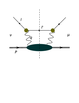
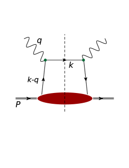
Figure 1: (Left) A representation of the DIS handbag diagram, illustrating the separate origins of the $L^{\mu\nu}$ and $W_{\mu\nu}$ tensors. (Right) The interaction of a nucleon with the virtual photon, as represented by the blue “blob” at left. The diagram is strictly leading twist, and follows from the photon scattering from an individual constituent quark, thereby giving the correlation functions $\Phi_{q,\bar{q}}$ of Eq. (21).

On general grounds, the hadronic tensor of Eq. (4) can be expanded explicitly in terms of hadronic current operators $J_{\mu}$ as suggested by the left-hand diagram of Fig. 2:

$$W_{\mu\nu}^{\alpha}\ (P,q)={1\over 2M}(2\pi)^{3}\ \sum_{X}\,\langle X|J_{\mu}^{\alpha}(0)|N\rangle^{*}\langle X|J_{\nu}^{\alpha}(0)|N\rangle\,\delta^{(4)}(P+q-k_{X})\ .$$ (8)

(We require the indices $\alpha=\{\gamma,\gamma Z,Z\}$ to specialize to specific neutral exchanges, as will become relevant for the treatment of electroweak processes in Chap. 2.)

We now more thoroughly explore the connection between the hadronic tensor $W_{\mu\nu}$ that enters the cross section for various QCD and electroweak processes and the more fundamental Compton amplitude $T_{\mu\nu}$. Writing Eq. (8) more carefully, one can obtain

$$2MW_{\mu\nu}(P,q)=\frac{1}{2\pi}\sum_{X}\int\frac{d^{3}k_{X}}{(2\pi)^{3}2k_{X}^{0}}\,(2\pi)^{4}\,\delta^{(4)}(q+P-k_{X})\,\langle P|J_{\mu}(0)|k_{X}\rangle\langle k_{X}|J_{\nu}(0)|P\rangle\ ,$$ (9)

such that the Fourier transformation of the 4-dimensional $\delta$-function given by

$$\delta^{(4)}(q+P-k_{X})=\frac{1}{(2\pi)^{4}}\int d^{4}\xi\,\exp\left(i[q+P-k_{X}]\cdot\xi\right)$$ (10)

permits a translation of the current operators in Eq. (9). This is allowed by the gauge invariance of the lagrangian from which the Compton amplitude is derived, which in turn implies a current conservation $\partial^{\mu}J_{\mu}\equiv 0$. Provided that the currents of Eq. (9) possess a leading twist bilinear form of $J_{\mu}(0)=\bar{\psi}(0)\,\Gamma_{\mu}\,\psi(0)$ for some Dirac structure $\Gamma_{\mu}$ (e.g., $\Gamma_{\mu}=\gamma_{\mu}$), we may make use of

$$e^{-ik_{X}\cdot\xi}\,\psi(0)\,|k_{X}\rangle =\psi(\xi)\,|k_{X}\rangle\ ,\ \ \ \ \ \ \ \ \langle P|\,\bar{\psi}(0)\,e^{+iP\cdot\xi}=\langle P|\,\bar{\psi}(\xi)\ ,$$ (11)

to rewrite Eq. (9) as

$$2MW_{\mu\nu}(P,q)=\frac{1}{2\pi}\int d^{4}\xi e^{iq\cdot\xi}\,\langle P|J_{\mu}(\xi)\,J_{\nu}(0)|P\rangle\ .$$ (12)

We have exploited the completeness of intermediate states in the cut “blob” of the Compton amplitude — i.e.,

$${1\over(2\pi)^{3}}\ \sum_{X}\ \frac{d^{3}k_{X}}{2k_{X}^{0}}\,|k_{X}\rangle\langle k_{X}|\ \equiv\ \mathbf{1}\ .$$ (13)

As a general consequence of the QFT optical theorem, this connects immediately to the matrix elements of the forward virtual Compton amplitude via

$$W_{\mu\nu}=\frac{1}{\pi}\ \mathrm{Im}\ T_{\mu\nu}\ \equiv\ \frac{1}{\pi}\ \mathrm{disc}\ T_{\mu\nu}\ ,$$ (14)

viz.

$$T_{\mu\nu} =i\,\int d^{4}\xi\,\exp(iq\cdot\xi)\langle N(p)|T\,\,J_{\mu}(\xi)\ J_{\nu}(0)|N(p)\rangle\ ,$$

$$=i\,\int d^{4}\xi\,\exp(iq\cdot\xi)\langle N(p)|\ [J_{\mu}(\xi),J_{\nu}(0)]|\ N(p)\rangle\ .$$ (15)

This can be seen through the canonical procedure: application of the Cutkosky rules [23] to the cut Compton amplitude, as illustrated in Fig. 2.

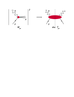
Figure 2: An illustration of the Cutkosky procedure, and the relation between the inclusive DIS process (left) and the cut Compton amplitude $\mathrm{disc}\,T_{\mu\nu}$ (right).

Schematically, the unitarity of the $S$-matrix $S^{\dagger}S\equiv 1$ also constrains the associated $T$-matrix due to the definition $S\mathrel{\vbox{\hbox{\scriptsize.}\hbox{\scriptsize.}}}=1+iT$. The field-theoretic analogue of this relation is precisely what is shown diagrammatically in Fig. 2. The gist of the fundamental procedure of [23] is that the discontinuity induced by the real axis branch cut in the exchange momenta $k_{X}$ of the Compton ‘blob’ in Fig. 2 can be accessed by replacing the internal integrations as

$$\int\ {d^{4}k_{X}\over(2\pi)^{4}}\ \rightarrow\ \int\ {d^{4}k_{X}\over(2\pi)^{4}}\ (2\pi)^{4}\ \delta^{(4)}\left(P+q-k_{X}\right)\ {1\over k^{2}_{X}-m^{2}+i\epsilon}\ ;$$ (16)

without loss of generality, we have assumed the exchanged momentum of the Compton ‘blob’ to be carried by scalar constituents — hence the explicit propagator of Eq. (16). By the residue theorem applied in the complex $k_{X}$ plane, we may thus isolate the discontinuity across the real axis $k_{X}>2m$ branch cut by placing the $k_{X}$ propagator on its mass-shell:

$${1\over k^{2}_{X}-m^{2}+i\epsilon}\ \rightarrow\ -2\pi i\ \delta(k^{2}_{X}-m^{2})\ ,$$ (17)

with the result of this scheme being the desired integration measure; that is,

$$\int\ dk^{0}_{X}\ {d^{3}k_{X}\over(2\pi)^{3}}\ (2\pi)^{4}\ \delta^{(4)} \left(P+q-k_{X}\right)\ \delta(k^{2}_{X}-m^{2})\$$

$$=\ {1\over(2\pi)^{3}}\ \int\ {d^{3}k_{X}\over 2k^{0}_{X}}\ (2\pi)^{4}\ \delta^{(4)}(P+q-k_{X})\ .$$ (18)

In fact, when wedded to the hadronic transition matrix elements $\langle P|J_{\mu}(0)|k_{X}\rangle\langle k_{X}|J_{\nu}(0)|P\rangle$ and incoherently summed over $X$ this result is consistent with Eq. (9), thus formalizing the connection between $W_{\mu\nu}$ and the operator structure of $T_{\mu\nu}$.

We shall proceed further by deconstructing $T_{\mu\nu}$ in terms of local current operators in Sec. 3. At the same time, in anticipation of subsequent developments within this thesis we note that a straightforward extension of the preceding formalism connects the hadronic tensor $W_{\mu\nu}$ to the internal quark-quark correlation functions that will be the subject of later modeling attempts, particularly those of Chap. 4.

We can follow the same Cutkosky paradigm as just outlined for the single nucleon example, but modify the handbag diagram to incorporate simple scattering from constituent quarks [24] of $4$-momentum $k$ as indicated in the right diagram of Fig. 1; the quark-level $W_{\mu\nu}$ tensor then becomes

$$2MW_{\mu\nu}\ =\ e^{2}_{q}\ \sum_{X}\ \int{d^{3}k_{X}\over(2\pi)^{3}\ 2k^{0}_{X}}\ \int d^{4}k\ \delta(k^{2}-m^{2})\ \theta(k^{0}-m)\ \delta^{(4)}(P+q-k_{X}-k)$$

$$\times\bigg{\{}\langle P|\ \bar{\psi}(0)\ |k_{X}\rangle\langle k_{X}|\ \psi(0)\ |P\rangle\ \gamma_{\mu}\ (\not{k}+m)\gamma_{\nu}\$$

$$\,\,\,\,\,-\ \langle P|\ \psi(0)\ |k_{X}\rangle\langle k_{X}|\ \bar{\psi}(0)\ |P\rangle\ \gamma_{\nu}\ (-\not{k}+m)\gamma_{\mu}\bigg{\}}\ .$$ (19)

If we repeat some of the same manipulations used to rewrite Eq. (9), this can be rendered as

$$2MW_{\mu\nu}\ =\ e^{2}_{q}\ \int d^{4}k\ \delta(k^{2}-m^{2})\ \theta(k^{0}-m)\ \int{d^{4}\xi\over(2\pi)^{4}}\ e^{-i(q-k)\cdot\xi}$$

$$\times\bigg{\{}\langle P|\ \bar{\psi}(\xi)\ \psi(0)\ |P\rangle\gamma_{\mu}\ (\not{k}+m)\gamma_{\nu}\$$

$$\,\,\,\,\,-\ \langle P|\ \psi(\xi)\ \bar{\psi}(0)\ |P\rangle\gamma_{\nu}\ (-\not{k}+m)\gamma_{\mu}\bigg{\}}\ ;$$ (20)

moreover, a simple inspection of the last equation suggests a compact form for the quark-level correlation functions. Evidently, they are

$$\Phi_{q}(P,k,q)\ =\ \int{d^{4}\xi\over(2\pi)^{4}}\ e^{-i(q-k)\cdot\xi}\,\,\langle P|\ \bar{\psi}(\xi)\ \psi(0)\ |P\rangle\ ,$$ (21a)

$$\Phi_{\bar{q}}(P,k,q)\ =\ \int{d^{4}\xi\over(2\pi)^{4}}\ e^{-i(q-k)\cdot\xi}\,\,\langle P|\ \psi(\xi)\ \bar{\psi}(0)\ |P\rangle\ .$$ (21b)

The existence of the correlators $\Phi_{q,\bar{q}}$ implies the validity the quark-parton model expressions we shall develop later in this thesis for the structure functions that emerge from $W_{\mu\nu}$. In essence, it is the objects $\Phi^{q,\bar{q}}$ that encode the nonperturbative long-distance correlations of quarks in the nucleon. It is these that remain beyond first principles computations in QCD, and hence are among the main goals of DIS and other experiments.

Next, in Sec. 2 we turn to the Compton amplitude in the real $Q^{2}=0$ limit. This will be explored in the context of dispersive Kramers-Krönig relations that enable one to extract surprising electromagnetic properties of the nucleon from the asymptotic (i.e., $\nu\to\infty$) behavior of the $\gamma N\rightarrow\gamma N$ reaction. Following this, in Sec. 3 we discuss basic features of DIS amplitudes in the operator product expansion (OPE) framework, which permits the twist decomposition of the hadronic observables that are a principal focus of this thesis. This treatment, with its scale-dependent factorization of short- from long-distance physics, will be in sharp contrast to the $Q^{2}=0$ techniques of Sec. 2.

2 Compton Scattering in the $Q^{2}=0$ limit

In the last section, we examined the relation between the DIS amplitude and analytic properties of the virtual Compton diagram. We continue that analysis in the present section by considering the Compton amplitude in the different setting of exclusive photoproduction reactions of the form $\gamma N\rightarrow\gamma N$, outlining the results of a recent publication [25]. In such situations both the initial and final state photons are purely real, and the associated forward (i.e., $q=q^{\prime}$) amplitude consequently selects uniquely constrained hadronic matrix elements. In particular, such physics is especially amenable at higher energies to Regge theory as mentioned in Chap. The nonperturbative structure of hadrons, hence offering a means of identifying possible dualities connecting short-distance physics to long-range dynamics. Moreover, for asymptotic photon energies ($\nu\to\infty$) the photon can couple locally to the constituent quark currents of the nucleon as depicted in Fig. 3, resulting in a universal (i.e., energy-independent) contribution to the scattering amplitude that has historically been thought to originate with a $J=0$ Regge pole [28, 29]. This observation is driven by the logic that the pointlike quark-photon vertex of Fig. 3 is dominated by spin-$0$ behavior, and would therefore be incorporated using the Regge language of Eq. (1) as an $\alpha_{J=0}(t=0)\equiv 0$ contribution to the forward Compton amplitude — an energy-independent constant. Making a precise measurement of the $J=0$ pole has thus been a strong object of interest for some decades, as doing so amounts to a basic test of the properties of QCD; this is because the $J=0$ pole contains information about the basic, energy-independent structure of the coupling of photons to the fundamental sources of electromagnetic charge within the theory — the constituent quarks [29].

There have in fact been a number of studies which have attempted to extract the $J=0$ pole; these have arrived at various numerical results more-or-less consistent with the Thomson term, $\mathrm{Re}\,T_{1}(0)=-3\,\mu$b$\cdot$GeV. These include the pioneering work of Damashek and Gilman [28], as well as results found in [30] and [31] ($\mathrm{Re}\,T_{1}^{J=0}=(-3\pm 2)\mu{\rm b\cdot GeV}$) and a slightly later study [32] ($\mathrm{Re}\,T_{1}^{J=0}=(-3^{+4}_{-5})\mu{\rm b\cdot GeV}$).

The advent of higher energy data at $\nu\gtrsim 10$ TeV, however, has made a re-analysis timely. In our recent calculation [25], a new attempt was made to carefully extract the fixed $J=0$ contribution in the spirit of [28], as well as to construct a series of consistent finite-energy sum rules (FESRs) on the basis of energy scale separation, by which we refer to the qualitatively distinct behaviors of the total photoproduction cross section that dominate within well-separated energy regimes. After a brief discussion of the basic theory, we therefore present a novel determination of the $J=0$ contribution, which indeed suggests a difference between the nucleon Thomson term and the quark-level fixed pole.

1 The Real Compton Amplitude

Real photon scattering is in fact simply a limit of the virtual photon case discussed in Sec. 1, corresponding to $Q^{2}\rightarrow 0$. More formally, in this special circumstance we make the following kinematical definitions: for real photons we take the $4$-momentum to be $q^{\mu}=(\nu,{\bf q})$ such that $q^{2}=\nu^{2}-{\bf q}^{2}=-Q^{2}\equiv 0$; the corresponding polarization vectors are then $\epsilon^{\mu}=(0,\bm{\epsilon})$. As before, the photon energy is $\nu=P\cdot q/M$. For our purposes, the object of dispersion relations at finite energy are the Compton amplitudes — especially for the nucleon spin-averaged process. These amplitudes reside within the Compton T-matrix, which may be taken from the Compton tensor of Eq. (15) after the appropriate contractions:

$$\mathscr{T}=e^{2}\,\epsilon^{\prime*\mu}\epsilon^{\nu}\,T_{\mu\nu}\ .$$ (22)

In the forward limit, we have $q=q^{\prime}$ and may expand the RHS of the last expression as

$$e^{2}\,T_{\mu\nu} =\bar{u}_{N}(P^{\prime})\,\big{(}T_{1}(\nu)\,g_{\mu\nu}+iT_{2}(\nu)\,\sigma_{\mu\nu}\big{)}\,u_{N}(P)\ ,$$

$$\mathscr{T} =8\pi M\,\bar{u}_{N}(P^{\prime})\,\big{(}\bm{\epsilon}^{\prime*}\cdot\bm{\epsilon}\,T_{1}(\nu)\,+\,i\sigma\cdot[\bm{\epsilon}^{\prime*}\times\bm{\epsilon}]\,iT_{2}(\nu)\big{)}\,u_{N}(P)\ .$$ (23)

Within this last expression, the simple spin-averaged Compton amplitude $T_{1}(\nu)$ contains much information bearing upon nucleon substructure, some of which has been newly extracted in our analysis [25]. The fact that $T_{1}(\nu)$ is an analytic function of the complex parameter $\nu$ implies this information can be accessed via the well-known Kramers-Krönig relations.

Generically, for a function $f(z)=f_{1}(z)+if_{2}(z)$ analytic in the upper-half complex plane, one can show [26] by the residue theorem that

$$f_{1}(z)={1\over\pi}\mathcal{P}\!\!\!\int\limits_{-\infty}^{\infty}dz^{\prime}\,{f_{2}(z^{\prime})\over z^{\prime}-z}\ .$$ (24)

If an odd behavior $f_{2}(-z)=-f_{2}(z)$ is ascribed to the imaginary part, several straightforward manipulations yield

$$f_{1}(z) ={1\over\pi}\mathcal{P}\!\!\!\int\limits_{-\infty}^{\infty}dz^{\prime}\,{z^{\prime}f_{2}(z^{\prime})\over z^{\prime 2}-z^{2}}+{z\over\pi}\mathcal{P}\!\!\!\int\limits_{-\infty}^{\infty}dz^{\prime}\,{f_{2}(z^{\prime})\over z^{\prime 2}-z^{2}}$$

$$={1\over\pi}\mathcal{P}\!\!\int\limits_{0}^{\infty}dz^{\prime 2}\,{f_{2}(z^{\prime})\over z^{\prime 2}-z^{2}}\ .$$ (25)

The finite behavior of the last integral in the $z\to\infty$ may be ensured by implementing a subtraction of the form $[f_{1}(z)-f_{1}(0)]/z^{2}$, which provides the once-subtracted dispersion relation we require —

$$f_{1}(z)=f_{1}(0)\,+\,{z^{2}\over\pi}\mathcal{P}\!\!\int\limits_{0}^{\infty}{dz^{\prime 2}\over z^{\prime 2}}\,{f_{2}(z^{\prime})\over z^{\prime 2}-z^{2}}\ ,$$ (26)

where the oddness of $f_{2}$ has ensured $f_{2}(0)=0$.

Figure 3: The fixed-pole contribution to the Compton amplitude may arise due to an effective, local two-photon coupling to elementary constituents within the proton.

Depending essentially only upon its analyticity and unitarity, the spin-averaged forward Compton scattering amplitude $T_{1}(\nu)$ of Eq. (23) can be cast into such a dispersive relation. Identifying the subtraction constant as the standard low-energy Thomson limit, the ‘master formula’ of this analysis follows:

$${\rm Re}\,T_{1}(\nu) =-\frac{Z^{2}}{A^{2}}\frac{\alpha}{M}+\frac{\nu^{2}}{\pi}\int_{0}^{\infty}\frac{d\nu^{\prime 2}}{\nu^{\prime 2}(\nu^{\prime 2}-\nu^{2})}{\rm Im}\,T_{1}(\nu^{\prime})$$

$$=-\frac{Z^{2}}{A^{2}}\frac{\alpha}{M}+\frac{\nu^{2}}{2\pi^{2}}\int_{0}^{\infty}\frac{d\nu^{\prime}}{\nu^{\prime 2}-\nu^{2}}\sigma(\nu^{\prime})\ .$$ (27)

where for convenience we have suppressed the explicit principal value $\mathcal{P}$ notation in Eq. (1) and the following. Also, for generality, we normalize to the mass number $A$. The second line of Eq. (1) emerges after a simple application of the optical theorem for real scattering

$${\rm Im}\,T(\nu) = \frac{\nu}{4\pi}\sigma(\nu)\ ,$$ (28)

which is in clear analogy with Eq. (14). That the subtraction constant in the dispersion relations of Eq. (1) should go as $T_{1}(0)=-(Z^{2}\alpha)\big{/}(A^{2}M)$ is required by the $\nu\to 0$ behavior of $T_{1}(\nu)$: namely, in the infrared limit the electromagnetic probe can only be sensitive to ‘global’ properties of the target, e.g., its charge and mass. This is precisely the Thomson term.

With this we pause momentarily to take stock of the significance of the last few deductions. For functions which are analytic in the upper-half of the complex plane, dispersion relations can be written down which connect their real and imaginary parts. That this can be done in the context of scattering theory for complex amplitudes implies their causal structure, which by the optical theorem permits observable cross sections to be related to the real part of the underlying amplitude as we have done in Eq. (1). This property allows us to analyze the contributions to $\mathrm{Re}\,T_{1}(\nu)$ using photoproduction measurements, and specifically, constrain the $J=0$ pole $\mathrm{Re}\,T_{1}^{J=0}(\nu)$.

2 Finite-Energy Sum Rules

By construction, the dispersive integral of Eq. (1) strictly includes photo-absorption cross sections all the way up to infinite energy; however, the approximate scale separation evident in Fig. 4 for the ²⁰⁷Pb cross section $\sigma_{T}(\nu)$ between the nuclear ($\nu\lesssim m_{\pi}$) and hadronic ($\nu\lesssim 2$ GeV) domains allows us to approximate the integral with a more restricted range of photo-absorption data. That is to say that the $\nu\to\infty$ contribution we aim to extract for perturbatively free partons has a corresponding analogue at lower energies; in this case, at energies sufficiently large relative to the giant dipole resonances (GDR) of Fig. 4, the nuclear Compton amplitude is dominated by local, pointlike interactions with individual constituent nucleons.

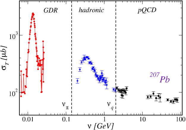
Figure 4: Scale separation is evident in the photo-absorption cross section for ²⁰⁷Pb. Data are taken from [34, 35, 36, 37, 38] and show the distinct regimes in $\nu$ for which scattering is predominantly from collective nuclei (giving rise to the GDR phenomenon), constituent nucleons, and pQCD quarks/gluons.

As we now demonstrate, this observation leads to the famous nuclear photo-absorption FESR due to Thomas, Reiche, and Kuhn (TRK) [33, 27]. Again, as shown in Fig. 4, nuclear deformation resonances (i.e., GDRs) saturate the photo-absorption cross section for $\nu\lesssim E_{\max}\approx 30$ MeV, such that we may compute the dispersive relation of Eq. (1) up to $\nu_{max}\lesssim m_{\pi}$, which approximately demarcates the purely nuclear physics from the hadronic scale beyond which single-nucleon resonances primarily contribute to the cross section,

$${\rm Re}\,T(\nu_{max}) \approx\ -\frac{Z^{2}}{A^{2}}\frac{\alpha}{M}-\frac{1}{2\pi^{2}}\int_{0}^{E_{max}}d\nu^{\prime}\sigma(\nu^{\prime})$$

$$\approx\ -\frac{Z}{A}\frac{\alpha}{M}\,\,\,\,\,\,\,\iff\,\,\,\,\,\,\,\nu_{max}\lesssim m_{\pi}\ .$$ (29)

Taking note that $\alpha/M\approx 3.03\mbox{ mb~{}MeV}$, as well as the assumption in the previous relation that the low-energy scattering is controlled by coherent interactions with individual nucleons, the TRK sum rule appears following some trivial reconfigurations —

$$\int_{0}^{E_{max}}d\nu\sigma(\nu)=2\pi^{2}\frac{NZ}{A^{2}}\frac{\alpha}{M}\approx 60\frac{NZ}{A^{2}}\mathrm{mb~{}MeV}\ ,$$ (30)

which has been found to hold at the $\sim 30$% level for an array of nuclei. Actually, the integration on the LHS of Eq. (29) is only approximately consistent with the dispersion relation of Eq. (1), and is obtained using an expansion of the form

$$\nu^{2}\int_{0}^{E_{max}}\!\!\!\!\!\!d\nu^{\prime}\frac{\sigma(\nu^{\prime})}{\nu^{2}-\nu^{\prime 2}}=\left[1+\frac{\langle\nu^{2}\rangle}{\nu^{2}}+\dots\right]\int_{0}^{E_{max}}\!\!\!\!\!\!d\nu^{\prime}\sigma(\nu^{\prime})\ ,$$ (31)

which is a sound approximation at first order so long as the spectrum-averaged mean squared energy satisfies

$$\langle\nu^{2}\rangle\ =\ \left(\int_{0}^{E_{max}}d\nu^{\prime}\ \nu^{\prime 2}\sigma(\nu^{\prime})\right)\Bigg{/}\left(\int_{0}^{E_{max}}d\nu^{\prime}\ \sigma(\nu^{\prime})\right)\ \ll\ 1\ .$$ (32)

For typical nuclei the first-order correction term of Eq. (31) represents a $\sim$10% effect, and neglecting it is therefore acceptable for the illustrative purposes here.

The arguments leading to the TRK sum rule are by no means unique, and readily generalize to the higher energies of the nucleon excitation (i.e., resonance) region, which roughly corresponds to $m_{\pi}\lesssim\nu\lesssim 2$ GeV. Beyond this kinematical regime, resonance excitations vanish as seen in Fig. 4, and the photo-production cross section is describable with a slow-varying background. Physically, this qualitative behavior is attributable to incoherent scattering off the constituent quarks of the nucleon. Building upon the analogy with Eq. (29), we therefore write down a FESR driven by scattering from constituent quarks:

$${\rm Re}\,T^{{\scriptscriptstyle{CQM}}}_{1}\equiv\mbox{Re}\,T_{1}(\nu_{max}) \approx -\frac{1}{A}\sum_{q\in A}\frac{\alpha}{m_{q}}e_{q}^{2}$$ (33)

$$= -\frac{3Z+2N}{A}\frac{\alpha}{M}\ .$$

Though tempting, it is not enough to proceed exactly as before with the TRK relation by simply associating ${\rm Re}\,T^{{\scriptscriptstyle{CQM}}}_{1}$ with the nuclear Thomson term of Eq. (29) added to the photo-absorption cross section integrated up to a large energy $E_{max}\gtrsim 2$ GeV relative to the nucleon resonance region. The simple reason for this is the high energy behavior of $\sigma_{T}(\nu)$, which, rather than vanishing, instead monotonically approaches the analytic Froissart bound [39] as seen in Fig. 5. Such an increase in the cross section can be understood as a feature of scattering from the asymptotically free partons of pQCD; as it happens, the $\nu$ dependence of these dynamics is ideally suited to Regge theory as already mentioned in Eq. (1). We explicitly model the contributions of reggeon and pomeron exchange to the cross section as

$$\sigma^{R+\mathbb{P}}(\nu)=\sigma^{R}_{T}+\sigma^{\mathbb{P}}_{T}=\sum_{i=R,\mathbb{P}}c_{i}\left(\frac{\nu}{\mbox{1 GeV}}\right)^{\alpha_{i}(0)-1}\ ,$$ (34)

where for dimensional reasons we include explicit factors of 1 GeV, and the pomeron and reggeon contributions are fixed by standard numerical choices for the trajectory intercepts $\alpha_{R}(0)=0.5$ and $\alpha_{\mathbb{P}}(0)=1.097$, respectively; we also again normalize to nucleon number for generality. These cross sections may be related to complex amplitudes of the form

$$T_{1}^{R+\mathbb{P}}(\nu)=T_{1}^{R}+T_{1}^{\mathbb{P}} =-\sum_{i=R,\mathbb{P}}\frac{c_{i}}{4\pi}\frac{1+e^{-i\pi\alpha_{i}(0)}}{\sin\pi\alpha_{i}(0)}\nu^{\alpha_{i}(0)}$$

$$=\frac{\nu^{2}}{2\pi^{2}}\int_{0}^{\infty}\frac{d\nu^{\prime}}{\nu^{\prime 2}-\nu^{2}}\sigma^{R+\mathbb{P}}(\nu^{\prime})\ .$$ (35)

We may therefore rewrite Eq. (1) by simply adding and subtracting the high energy contributions of Eqs. (34) and (35), hence leading to

$$\mbox{Re}\,T_{1}(\nu) =-\frac{Z^{2}}{A^{2}}\frac{\alpha}{M}+\frac{\nu^{2}}{2\pi^{2}}\int_{0}^{\infty}d\nu^{\prime}\frac{\sigma(\nu^{\prime})-\sigma^{R+\mathbb{P}}(\nu^{\prime})}{\nu^{\prime 2}-\nu^{2}}+\mbox{Re}\,T_{1}^{R+\mathbb{P}}(\nu)$$ (36)

$$=-\frac{Z^{2}}{A^{2}}\frac{\alpha}{M}-\frac{1}{2\pi^{2}}\int_{0}^{E}d\nu^{\prime}\sigma(\nu^{\prime})+\sum_{i=R,\mathbb{P}}\frac{c_{i}\mbox{GeV}}{2\pi^{2}\alpha_{i}(0)}\left(\frac{E}{\mbox{1 GeV}}\right)^{\alpha_{i}(0)}+\,\mbox{Re}\,T_{1}^{R+\mathbb{P}}(\nu)\ ,$$

where we obtain the second line by taking the asymptotic limit $\nu\to\infty$ to evaluate the subtraction in the integrand of the first line. In Eq. (36) $E\sim 2$ GeV is the energy beyond which the difference between the data $\sigma(\nu)$ and the high-energy asymptotic form $\sigma^{R+\mathbb{P}}(\nu)$ is negligible.

We proceed by identifying the constituent quark analog of the TRK constant computed in Eq. (33) as the contribution from scattering off bound quarks; doing so, we may then recast the LHS of Eq. (36) as

$$\mbox{Re}\,T_{1}(\nu)=\mbox{Re}\,T_{1}^{{\scriptscriptstyle{CQM}}}\,+\,\frac{c_{\mathbb{P}}\mbox{GeV}}{2\pi^{2}\alpha_{P}(0)}\left(\frac{E}{\mbox{1 GeV}}\right)^{\alpha_{\mathbb{P}}(0)}\,+\,\mbox{Re}\,T_{1}^{R+\mathbb{P}}(\nu)\ ,$$ (37)

thereby leading to a new phenomenological FESR at quark-level after several rearrangements:

$$\mbox{Re}\,T_{1}^{{\scriptscriptstyle{CQM}}} =-\frac{Z^{2}}{A^{2}}\frac{\alpha}{M}-\frac{1}{2\pi^{2}}\int_{0}^{E}d\nu^{\prime}\sigma(\nu^{\prime})+\frac{c_{R}\mbox{GeV}}{2\pi^{2}\alpha_{R}(0)}\left(\frac{E}{\mbox{1 GeV}}\right)^{\alpha_{R}(0)}\,\,\,\implies$$

$$-\left(2+\frac{ZN}{A^{2}}\right)\frac{\alpha}{M} =-\frac{1}{2\pi^{2}}\int_{0}^{E}d\nu^{\prime}\sigma(\nu^{\prime})+\frac{c_{R}\mbox{GeV}}{2\pi^{2}\alpha_{R}(0)}\left(\frac{E}{\mbox{1 GeV}}\right)^{\alpha_{R}(0)}\ .$$ (38)

We note that the pomeron term must be included explicitly in Eq. (37) to account for the fact that $\mathbb{P}$-exchanges possess quantum numbers consistent with the vacuum (putatively arising from gluonic pQCD mechanisms), and therefore cannot directly contribute to $\mbox{Re}\,T_{1}^{{\scriptscriptstyle{CQM}}}$.

Aside from this novel FESR, we may also exploit Eq. (36) to determine the scale independent $J=0$ pole described at the start of Sec. 2; namely, this is the difference between the complete forward Compton amplitude up through the excitation region and the smooth Regge theory background:

$$\mbox{Re}\,T_{1}^{J=0} \mathrel{\vbox{\hbox{\scriptsize.}\hbox{\scriptsize.}}}=\lim_{\nu\to\infty}[\mbox{Re}\,T_{1}(\nu)-\mbox{Re}\,T_{1}^{R+\mathbb{P}}(\nu)]$$

$$=-\frac{Z^{2}}{A^{2}}\frac{\alpha}{M}-\frac{1}{2\pi^{2}}\int_{0}^{E}d\nu^{\prime}\sigma(\nu^{\prime})+\sum_{i=R,\mathbb{P}}\frac{c_{i}\mbox{GeV}}{2\pi^{2}\alpha_{i}(0)}\left(\frac{E}{\mbox{1 GeV}}\right)^{\alpha_{i}(0)}\ .$$ (39)

3 The $J=0$ Pole and CQM FESR

To extract a numerical determination of the $J=0$ fixed pole from the FESR given in Eq. (39), it is first necessary to parametrize the $\nu$ dependence of the hadronic cross-section — we do so by fitting a sum of Breit-Wigner resonances over a smooth background [25]. Moreover, the Regge theory background is chosen so that it explicitly matches onto the Regge cross section,

$$\sigma^{R+\mathbb{P}}(\nu)=\left(1-e^{-\frac{2(\nu-\nu_{\pi})}{M}}\right)\,\cdot\,\left[c_{R}\left(\frac{\nu}{1\,\mathrm{GeV}}\right)^{0.097}\,+\,c_{\mathbb{P}}\left(\frac{\nu}{1\,\mathrm{GeV}}\right)^{-0.5}\right]\ ,$$ (40)

where the prefactor ensures that the background vanishes at pion threshold.

As mentioned, we take the Regge intercepts from previous fits to photo-absorption data on the proton [41], with the consequent high-fidelity description of the global proton photo-production data shown in Fig. 5. Constraining the model in Eq. (40) to modern data, which now extend to larger values of $\nu$, leads to a significant enhancement in the contributions from reggeon exhange, and we find the parameters $c_{R}=68.0\mu$b, and $c_{\mathbb{P}}=99.0\mu$b most adequately adapt the Regge background to the $\nu\gtrsim 2$ GeV data. This contrasts significantly compared to fits from the benchmark work by Damashek and Gilman [28], which at the time lacked the high-energy rise due to pomeron exchange:

$$\sigma^{R+\mathbb{P}}(\nu)=\left(96.6\ +\ 70.2\ \left[{\nu\over 1\ \mathrm{GeV}}\right]^{-1/2}\right)\ \mu\mathrm{b}\ ;$$ (41)

improvements in data at high $\nu$ thus lead to a rather different numerical description of photoproduction.

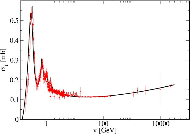
Figure 5: The fit to the total photoproduction cross section off the proton (red dots) using a sum of Breit-Wigner resonances in the low-energy region, and a continuous Regge background extended from higher energies (solid curve).

Assembling these various elements, we are able to estimate the $J=0$ fixed pole, now finding [25]

$${\rm Re}\,T^{J=0}_{1}\ =\ (-0.72\pm 0.35)\ \mu{\rm b\,GeV}\ ;$$ (42)

when connected to modern high-energy data, the dispersive approach therefore produces a fixed pole contribution which is markedly different from previous estimates [28, 30, 31, 32]. Given that these had been consistent with the standard Thomson term result Re $T_{1}(0)=-3.03\mu$bGeV as summarized at the start of Sec. 2, this new discrepancy is for the first time confirmational that the main contribution to Eq. (39) does not come from the coherent nucleonic Thomson term alone, but from local interactions of the type shown in Fig. 3. Tracing the separate origin of these contributions can in principle be accomplished by means of the CQM FESR developed in Eq. (38), for example, and urges additional analytic and experimental investigations of exclusive processes like $\gamma N\rightarrow\gamma N$.

3 The Operator Product Expansion

We conclude this chapter with a pedagogical overview of a computational technique of considerable utility in analyzing hadronic matrix elements. As it is these that encode the details of nonperturbative structure extracted in DIS, a brief description will help to contextualize the arguments of Chap. 2 – 3.

The hadronic tensor $W_{\mu\nu}$ of Eq. (12) is the Fourier transform of a time-ordered product of currents that possess a definite operator structure at the level of the bilinears $J_{\mu}(\xi)=\bar{\psi}(\xi)\,\Gamma_{\mu}\,\psi(\xi)$. Without much loss of generality, one might concisely state the object of QFT applied to hadronic structure as a program for understanding the inherently non-local correlations of constituent fields within the nucleon (for instance) in terms of specific local operators of definite dimension, spin, parity, etc. Of course, the nucleon is nonperturbative by nature, and the array of operators that contribute to the product $J_{\mu}(\xi)\,J_{\nu}(0)$ is in principle unbounded. To rectify this impasse, an expansion is required that provides a natural decomposition of the non-local product $J_{\mu}(\xi)\,J_{\nu}(0)$ in terms of local operators $\hat{\mathcal{O}}^{i}(0)$ in a fashion that gives a specific ordering. This is precisely the description of Wilson’s Operator Product Expansion (OPE) [42].

In broadest terms, the OPE implies the following separation: for two generic operators $\Omega_{1}(\xi_{1})$, $\Omega_{2}(\xi_{2})$, their product can be expanded as the sum

$$\Omega_{1}(\xi_{1})\,\Omega_{2}(\xi_{2})\, =\,\sum_{i}\,C_{i}(\xi_{1}-\xi_{2})\,\hat{\mathcal{O}}^{i}\left(\xi_{2}\right)\,\,\,\,\implies$$

$$J(\xi)\,J(0)\, =\,\sum_{i}\,C_{i}(\xi)\,\hat{\mathcal{O}}^{i}(0)\ ,$$ (43)

where the the sum over $i$ counts various operator structures, and the coefficients $C_{i}(\xi)$ are generally singular in the $\xi\rightarrow 0$ limit (in fact, the leading contributions to the OPE originate in the $\hat{\mathcal{O}}^{i}$ associated with coefficients $C_{i}(\xi)$ which are most singular for $\xi^{2}\sim 0$). Moreover, the scale dependence $Q^{2}$ relative to the renormalization parameter $\mu$ is fully contained within the coefficient functions, which satisfy the Callan-Symanzik renormalization group equation [43]

$$\left(\mu{\partial\over\partial\mu}+\beta(g){\partial\over\partial g}-\gamma^{N}\right)C^{N}\left({Q^{2}\over\mu^{2}},g\right)\,\equiv\,0\ ,$$ (44)

which requires knowledge of the QCD Beta function $\beta(g)$ [defined in Eq. (3)] and anomalous dimension $\gamma^{N}$.

Fundamentally, the OPE posits that the Fourier-transformed product of hadronic currents defined by Eq. (15) can be expanded in a closed set of Lorentz structures; these may be compiled as [44]

$$T_{\mu\nu} =\sum_{i,N}\ \bigg{[}\left(g_{\mu\nu}-{q_{\mu}q_{\nu}\over q^{2}}\right)\ q_{\mu_{1}}\dots q_{\mu_{N}}C^{N}_{L,i}\left({Q^{2}\over m^{2}},g^{2}\right)$$ (45)

$$+\ \left(g_{\mu\mu_{1}}q_{\nu}q_{\mu_{2}}+g_{\nu\mu_{2}}q_{\mu}q_{\mu_{1}}-g_{\mu\nu}q_{\mu_{1}}q_{\mu_{2}}+g_{\mu\mu_{1}}g_{\nu\mu_{2}}Q^{2}\right)q_{\mu_{3}}\dots q_{\mu_{N}}\ C^{N}_{2,i}\left({Q^{2}\over m^{2}},g^{2}\right)$$

$$-\ i\epsilon_{\mu\nu\alpha\beta}\ g_{\alpha\mu_{1}}q_{\beta}q_{\mu_{2}}\ \dots\ q_{\mu_{N}}\ C^{N}_{3,i}\left({Q^{2}\over m^{2}},g^{2}\right)\bigg{]}\,\,\times\,\,\bigg{(}{2\over Q^{2}}\bigg{)}^{N}\ \langle N(P)|\ \mathcal{O}^{\mu_{1}\dots\mu_{N}}_{i}(0)\ |N(P)\rangle\ .$$

Lorentz covariance allows the nucleon spin-averaged matrix elements of local operators to be expanded in the general form

$$\langle N(P)|\ \mathcal{O}^{\mu_{1}\dots\mu_{N}}_{i}(0)\ |N(P)\rangle\ =\ A^{(N)}_{i}\ \cdot\ \bigg{[}P^{\mu_{1}}\ P^{\mu_{2}}\ \dots\ P^{\mu_{N}}\bigg{]}\ -\{\ \mathrm{trace}\,\,\mathrm{terms}\ \}\ ,$$ (46)

in which the hadronic matrix elements of the operators $\mathcal{O}_{i}$ have been factorized from the momenta $P^{\mu_{1}}\ P^{\mu_{2}}\ \dots\ P^{\mu_{N}}$; also, in Eq. (46) ‘trace terms’ refers to combinations involving $g^{\mu_{a}\mu_{b}}$ that ensure the tracelessness of the final expansion. This full form is only necessary for a thorough treatment at leading twist which includes fully summed power corrections. Ignoring these for the sake of illustration at present (in fact they will be needed later in Chap. 3 to evaluate target mass effects), we insert the un-symmetrized expression of Eq. (46) [i.e., excluding the trace terms] into Eq. (45), leading to the desired combination of coefficient functions and hadronic matrix elements. A few simple tensor contractions are sufficient to yield

$$T_{\mu\nu}=\sum_{i,N}\ \bigg{[}\kappa^{L}_{\mu\nu}\ C^{N}_{L,i}(Q^{2})\ +\ \kappa^{2}_{\mu\nu}\ C^{N}_{2,i}(Q^{2})\ +\ \kappa^{3}_{\mu\nu}\ C^{N}_{3,i}(Q^{2})\bigg{]}\,\,\times\,\,\bigg{(}{1\over x}\bigg{)}^{N}\ A_{i}^{(N)}\ ,$$ (47)

where the rank-2 objects

$$\kappa^{L}_{\mu\nu}\ =\ g_{\mu\nu}+{q_{\mu}\ q_{\nu}\over Q^{2}}\ ,$$ (48a)

$$\kappa^{2}_{\mu\nu}\ =\ \left({P_{\mu}P_{\nu}\over\nu^{2}}\right){1\over Q^{2}}\ +\ \Big{(}P_{\mu}\ q_{\nu}+P_{\nu}\ q_{\mu}\Big{)}\Big{/}\nu\ -\ g_{\mu\nu}\ ,$$ (48b)

$$\kappa^{3}_{\mu\nu}\ =\ i\epsilon_{\mu\nu\alpha\beta}{P_{\alpha}\ q_{\beta}\over q}\ ,$$ (48c)

follow from the expression in Eq. (46) up to contributions from the trace terms, which are only relevant for higher power corrections in $(1/Q^{2})$. As mentioned, the role of these additional terms in generating target mass corrections will be discussed subsequently in Chap. 3.2.

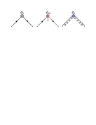
Figure 6: Leading twist operator structures $\mathcal{O}_{i}$ that contribute to the OPE of Eq. (45).

At leading twist, however, basic symmetries require that only three primary operator structures can contribute to the parton-level product of currents $J(\xi)\,J(0)$ [45]. These are the singlet current operator $i=S$

$$\mathcal{O}^{\mu_{1}\dots\mu_{N}}_{S}(0)\ ={i^{n-1}\over 2n!}\ \left(\gamma^{\mu_{1}}\ D^{\mu_{2}}\ \dots\ D^{\mu_{N}}\,\,+\mu_{a}\mu_{b}\,\,\,\mathit{permutations}\right)\ ,$$ (49)

non-singlet ($i=NS$)

$$\mathcal{O}^{\mu_{1}\dots\mu_{N}}_{NS}(0)\ ={i^{n-1}\over 2n!}\ \left(\gamma^{\mu_{1}}\ D^{\mu_{2}}\ \dots\ D^{\mu_{N}}\ \hat{\lambda}\,\,+\mu_{a}\mu_{b}\,\,\,\mathit{permutations}\right)\ ,$$ (50)

and tree-level couplings of the glue ($i=g$)

$$\mathcal{O}^{\mu_{1}\dots\mu_{N}}_{g}(0)\ ={i^{n-2}\over n!}\ \left(\hat{G}^{\mu_{1}\mu}\ D^{\mu_{2}}\ \dots\ D^{\mu_{N-1}}\ \hat{G}^{\mu_{N}}_{\mu}\,\,+\mu_{a}\mu_{b}\,\,\,\mathit{permutations}\right)\ ,$$ (51)

all of which are represented pictorially in Fig. 6.

The operator decomposition of hadronic currents is most easily studied in terms of the moments of DIS structure functions, which can be unfolded from Eq. (45) by again invoking the analyticity of $T_{\mu\nu}$. Employing the same logic we exploited in Sec. 2 to project the desired helicity amplitudes from the Compton amplitude, the residue theorem in the parameter $\omega=(1/x)\in\mathbb{C}$ implies

$${1\over 2\pi i}\ \oint_{C}\ \omega^{-N}\ T_{\mu\nu}\equiv\ {2\over\pi}\ \int_{1}^{\infty}\ d\omega\ \omega^{-N}\ \mathrm{Im}\,T_{\mu\nu}\ ;$$ (52)

the latter quantity on the RHS, $\mathrm{Im}\,T_{\mu\nu}$, can be related explicitly to the DIS structure functions we require on the grounds of Eq. (14). Again the Cauchy theorem allows the LHS of Eq. (52) to be evaluated term-wise, and a simple change of variables on the RHS gives

$${2\over\pi}\ \int_{1}^{\infty}\ d\omega\ \omega^{-N}\ \mathrm{Im}\,T_{\mu\nu}\ \rightarrow\ 2\ \int_{0}^{1}\ dx\cdot x^{N-2}\ W_{\mu\nu}\ .$$ (53)

With this, it is then enough to go term-by-term in the $\kappa_{\mu\nu}$ tensors of Eq. (47) and equate the various moments within Eq. (53); we thus get the leading twist moments $M^{N}(Q^{2})$:

$$M^{N}_{L/2}(Q^{2})\ =\ \int_{0}^{1}\ dx\cdot x^{N-2}\ F_{L/2}(x,Q^{2})\ =\ \sum_{i}\ A^{(N)}_{i}\cdot C^{N}_{L/2,\ i}(Q^{2})\ ,$$ (54a)

$$M^{N}_{3}(Q^{2})\ =\ \int_{0}^{1}\ dx\cdot x^{N-1}\ F_{3}(x,Q^{2})\ =\ A^{(N)}_{NS}\cdot C^{N}_{3,\ NS}(Q^{2})\ .$$ (54b)

The OPE therefore provides relations between the moments $M^{N}(Q^{2})$ of structure functions $F(x,Q^{2})$ and matrix elements $A^{(N)}_{i}$ of the operators $\mathcal{O}_{i}$ depicted in Fig. 6 at leading twist. The structure functions themselves may be obtained from Eq. (54) by applying an analytic transform, as we shall demonstrate for a specific example related to target mass corrections in Eq. (8) of Chap. 3.

All the more, the scale dependence in the formalism resides entirely within the calculable functions $C^{N}(Q^{2},g)$, which run according to Eq. (44). Thus, if the perturbatively calculable beta function and anomalous dimension are known, the dependence on $Q^{2}$ of the moments $M^{N}(Q^{2})$ can also be determined, and from that, the evolution of $F(x,Q^{2})$. To leading order in $\alpha_{s}$ the running of, e.g., moments of non-singlet structure functions like $F_{3}(x,Q^{2})$ can be written simply as [46]

$$M^{N,(0)}_{3}(Q^{2})\ =\ \left\{{\alpha_{s}(Q^{2})\over\alpha_{s}(\mu^{2})}\right\}^{\gamma^{N,(0)}_{NS}\Big{/}2\beta_{0}}\cdot M^{N}_{3}(\mu^{2})\ ,$$ (55)

where the parameter $\beta_{0}$ of the leading order beta function may be taken from Eq. (3) as$\beta_{0}\mathrel{\vbox{\hbox{\scriptsize.}\hbox{\scriptsize.}}}=11-2n_{F}/3$, and $\mu$ is an initial renormalization scale at which the OPE is applied. In particular, $\gamma^{N=1,(0)}_{NS}=0$ — a useful fact which guarantees the leading order scale invariance of non-singlet moments, including the valence quark distributions to be introduced in later chapters.

Chapter 2 Finite-$Q^{2}$ corrections in electroweak phenomenology

“Similarly, many a young man, hearing for the first time of the refraction of stellar light, has thought that doubt was cast on the whole of astronomy, whereas nothing is required but an easily effected and unimportant correction to put everything right again.”
      — Ernst Mach

As emphasized in the preceding chapters, energetic lepton-nucleon scattering has been the primary source of knowledge regarding the nucleon’s quark and gluon (i.e., parton) substructure. In keeping with the chronology we introduced in Chap. The nonperturbative structure of hadrons, the preponderance of this information has come from DIS of electrons (or muons), while neutrino DIS has yielded complementary constraints on valence and sea parton distribution functions (PDFs) via the weak current.

Though recent decades have seen increased activity, a less thoroughly explored method involves the interference of electromagnetic and weak currents, which is capable of selecting unique partonic flavor combinations — a quality attributable to the parity-violating operator structures involved. The interference approach consists of measuring the small $\gamma$–$Z^{0}$ amplitude in the neutral current DIS of a polarized electron from a hadron $h$, $\vec{e}\ h\to e\ X$. Because the axial current is sensitive to the polarization of the incident electron, measurement of the asymmetry between left- and right-hand polarized electrons is thus proportional to the $\gamma$–$Z^{0}$ interference amplitude.

As we alluded in the introductory chapter, 1970s parity-violating DIS (PVDIS) measurements were responsible for key early confirmations of the Standard Model (SM) of particle physics [48, 49]. All the more, after four decades experimental techniques are now sophisticated enough to enable the measurement of left-right asymmetries as small as a few parts-per-billion, while current and next-generation facilities will be able to upgrade the statistics of earlier experiments by an order of magnitude [50, 51].

Aside from these issues, precision studies in the electroweak sector have garnered special interest in recent years as the assault on the long-standing dark matter (DM) problem has grown more elaborate (as have other general tests of the SM). The SM inputs of the electroweak (EW) sector are conceivably sensitive to various potential non-SM dynamics. Often, this novel physics is imagined as arising from undiscovered processes that might predominate at some scale $\Lambda>\Lambda_{EW}$ beyond that of the EW sector, as hypothetically occurs (for example) in certain predictions of technicolor or other supersymmetric extensions of the SM, leptoquarks, composite fermions, etc; the resulting physics might then be encapsulated in new four-fermion contact interactions of the form [52]

$$\mathcal{L}^{BSM}_{eff}\ =\ {g^{2}\over(1+\delta)\,\Lambda}\sum_{i,j=L,R}\eta^{\psi}_{ij}\ \bar{e}_{i}\gamma_{\mu}e_{i}\,\cdot\,\bar{\psi}_{j}\gamma^{\mu}\psi_{j}\ ,$$ (1)

where $\psi$ can represent the Dirac fields of quarks or leptons, $\delta=0,1$ for $\psi=e,\,\neq e$, and the matrix elements $\eta^{\psi}_{ij}=\pm 1,0$. Concisely stated, the principal aim of modern searches for physics beyond the SM is to better constrain the scale $\Lambda$ and interaction strength $g$ that enter effective interactions of the type $\mathcal{L}^{BSM}_{eff}$ defined in Eq. (1), the existence of which would produce observable differences from the effective four-fermion interactions that can be computed within the standard EW theory as we illustrate shortly.

Experience teaches that the hypothetical signals for these novel dynamics would almost certainly require an unprecedented level of precision to access, and to provide this it is first necessary to understand the predictions of the SM electroweak theory for electron-nucleon DIS, as well as the potential power corrections and other nonperturbative effects that could complicate such experimental determinations.

1 The Electroweak Lagrangian

The $SU(2)\times U(1)$ GWS theory [53, 54] prescribes a self-contained form for the propagator structure and interactions within the EW sector. Using standard notation, the lagrangian for the left-handed ($\Psi$) and right-handed ($\psi$) fermion fields can be put down as

$$\mathcal{L}^{EW} =\sum_{i}\,\,\bar{\psi}_{i}\,\left(i\not{\partial}-m_{i}-{g\,m_{i}\mathcal{H}\over 2m_{W}}\right)\,\psi_{i}$$

$$-\sum_{i}\,\,\hat{q_{i}}\,\bar{\psi}_{i}\,\gamma^{\mu}\,\psi_{i}A_{\mu}$$

$$-{g\over 2\sqrt{2}}\sum_{i}\,\,\bar{\Psi}_{i}\,\gamma^{\mu}\mathcal{P}^{-}\left(T^{-}W^{-}_{\mu}+T^{+}W^{+}_{\mu}\right)\,\Psi_{i}$$

$$-{g\over 2\cos{\theta_{W}}}\sum_{i}\,\,\bar{\psi}_{i}\gamma^{\mu}\left(g_{V}^{i}-g_{A}^{i}\gamma^{5}\right)\psi_{i}\,Z_{\mu}\ ,$$ (2)

with $\hat{q}_{i}=e\cdot q_{i}$, where $q_{i}$ is the fractional charge of the $i^{th}$ fermion species. The projection operator we have taken to be $\mathcal{P}^{-}\mathrel{\vbox{\hbox{\scriptsize.}\hbox{\scriptsize.}}}=1-\gamma^{5}$, $\mathcal{H}$ is the Higgs field, $\theta_{W}$ the famous weak mixing angle first introduced by Weinberg [55], and $g$ represents the gauge coupling constant.

Unlike the singlet right-handed mass eigenstates $\psi$, the left-handed fields are doublets

$$\Psi=\left(\begin{array}[]{c}\nu_{i}\\ l^{-}_{i}\end{array}\right)\ ,\,\,\,\,\,\left(\begin{array}[]{c}u_{i}\\ d^{\prime}_{i}\end{array}\right)\ ,$$ (3)

which mix under the CKM matrix [56] in the latter case of the quark fields; this induces the flavor-mixing of the three quark generations, such that, for example, $d^{\prime}\approx V_{ud}d+V_{us}s$ after neglecting the heaviest generation.

With this, we can interpret the SM interactions provided by Eq. (2): the first, kinetic term contains the fermion propagators and Yukawa-type coupling following the Higgs’ spontaneous acquisition of a non-zero vacuum expectation value (VEV), whereas the second term codifies the electromagnetic photon-fermion coupling. The third and fourth terms provide the quark and lepton couplings to the gauge fields, which are of particular relevance for parity violation studies. For instance, using the definition of Eq. (3) for light quarks in Eq. (2) results in the charged current (CC) coupling

$$\mathcal{L}^{CC} ={-g\over 2\sqrt{2}}\,\sum_{i}\,\left(\bar{u}_{i},\bar{d}^{\prime}_{i}\right)\gamma^{\mu}\mathcal{P}^{-}\,\left[T^{-}W^{-}_{\mu}+T^{+}W^{+}_{\mu}\right]\,\left(\begin{array}[]{c}u_{i}\\ d^{\prime}_{i}\end{array}\right)$$ (6)

$$={-g\over 2\sqrt{2}}\,\Big{(}\bar{u}\gamma^{\mu}(1-\gamma^{5})d^{\prime}\,W^{+}_{\mu}\,\,+\,\,\bar{d}^{\prime}\gamma^{\mu}(1-\gamma^{5})u\,W^{-}_{\mu}\Big{)}\ ,$$ (7)

where again the mixed state $d^{\prime}$ is determined from CKM matrix elements as $d^{\prime}_{i}=\sum_{j}\,\mathcal{V}_{ij}d_{j}$. These considerations figure importantly in direct searches for parton-level violation of charge symmetry as discussed in Sec. 3.

The source of parity violation in neutral current (NC) electron scattering from hadrons is the $Z^{0}$ exchange mechanism; to describe this process, we require the quark and lepton couplings that can be taken from the fourth term of Eq. (2):

$$\mathcal{L}^{e}_{Z} =\ {-g\over 2\cos{\theta_{W}}}\,\bar{e}\,\gamma^{\mu}\left(g^{e}_{V}-g^{e}_{A}\gamma^{5}\right)e\,Z_{\mu}\ ,$$ (8a)

$$\mathcal{L}^{u}_{Z} =\ {-g\over 2\cos{\theta_{W}}}\,\bar{u}\,\gamma^{\mu}\left(g^{u}_{V}-g^{u}_{A}\gamma^{5}\right)u\,Z_{\mu}\ ,$$ (8b)

$$\mathcal{L}^{d}_{Z} =\ {-g\over 2\cos{\theta_{W}}}\,\bar{d}\,\gamma^{\mu}\left(g^{d}_{V}-g^{d}_{A}\gamma^{5}\right)d\,Z_{\mu}\ .$$ (8c)

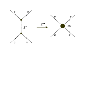
Figure 1: For $Q^{2}\ll m^{2}_{Z}$, the exchange mechanism at left can be used to compute the effective parity-violating interaction given in Eq. (12).

These interactions supply the vertex structure in the $Z^{0}$-exchange diagram in the LHS of Fig. 1. With them, we can compute an amplitude, which we call $A_{Z}$:

$$A_{Z} = \left({g^{2}\over 4\cos^{2}{\theta_{W}}}\right)\,\bar{e}\,\gamma^{\mu}\left(g^{e}_{V}-g^{e}_{A}\gamma^{5}\right)e\,Z_{\mu}\,Z_{\nu}\,\bar{u}\,\gamma^{\nu}\left(g^{u}_{V}-g^{u}_{A}\gamma^{5}\right)u\,\,+\,\,\{d\,\,\mathit{terms}\}$$ (9)

$$= \left({g^{2}\over 4\cos^{2}{\theta_{W}}}\right)\,\bar{e}\,\gamma^{\mu}\left(g^{e}_{V}-g^{e}_{A}\gamma^{5}\right)e\,\left[{g_{\mu\nu}\over k^{2}-m^{2}_{Z}+i\epsilon}\right]\,\bar{u}\,\gamma^{\nu}\left(g^{u}_{V}-g^{u}_{A}\gamma^{5}\right)u$$

$$\,\,\,\,\,\,\,\,\,\,\,\,\,\,\,\,\,\,\,\hskip 35.56593pt+\,\,\{d\ \ \mathrm{terms}\}\ ,$$

where we have used a Feynman gauge expression for the $Z^{0}$ propagator. The behavior of the amplitude in Eq. (9) under the parity operator ensures that only terms linear in $\gamma^{5}$ contribute to parity violation; taken together with a limit in which the exchange momentum of the $Z^{0}$ is small (i.e., , $k^{2}\ll m^{2}_{Z}$), this results in

$$A^{PV}_{Z} = \left({g^{2}\over 4\cos^{2}{\theta_{W}}}\right)\,\bar{e}\,\gamma^{\mu}\left(g^{e}_{V}-g^{e}_{A}\gamma^{5}\right)e\,\left[{-g_{\mu\nu}\over m^{2}_{Z}}\right]\,\bar{u}\,\gamma^{\nu}\left(g^{u}_{V}-g^{u}_{A}\gamma^{5}\right)u\,\,+\,\,\{d\,\,\mathit{terms}\}\,\,\,\implies$$ (10)

$$= \left({g^{2}\over 4m^{2}_{Z}\cos^{2}{\theta_{W}}}\right)\,\left[g^{e}_{V}\cdot g^{u}_{A}\,\bar{e}\,\gamma^{\mu}e\,\bar{u}\,\gamma_{\mu}\gamma^{5}\,u\,\,+g^{e}_{A}\cdot g^{u}_{V}\,\bar{e}\,\gamma^{\mu}\gamma^{5}e\,\bar{u}\,\gamma_{\mu}\,u\right]$$

$$\,\,\,\,\,\,\,\,\,\,\,\,\,\,\,\,\,\,\,\hskip 35.56593pt+\,\,\{d\ \ \mathrm{terms}\}\ .$$

This last expression amounts to an effective, parity-violating four-fermion lepton-quark interaction. In fact, after imposing the so-called ‘custodial’ symmetry $m^{2}_{W}=m^{2}_{Z}\cdot\cos^{2}{\theta_{W}}$, and using the canonical definition of the effective Fermi coupling

$${G_{F}\over\sqrt{2}}={g^{2}\over 8m^{2}_{W}}\approx{g^{2}\over 8m^{2}_{Z}\cos^{2}{\theta_{W}}}\ ,$$ (11)

a convenient form for the flavor $SU(2)$ parity-violating lagrangian presents itself:

$${\cal L}^{\rm PV}=\frac{G_{F}}{\sqrt{2}}\left[\bar{e}\gamma^{\mu}\gamma_{5}e\left(C_{1u}\bar{u}\gamma_{\mu}u+C_{1d}\bar{d}\gamma_{\mu}d\right)+\bar{e}\gamma^{\mu}e\left(C_{2u}\bar{u}\gamma_{\mu}\gamma_{5}u+C_{2d}\bar{d}\gamma_{\mu}\gamma_{5}d\right)\right]\ ,$$ (12)

in which the tree-level electroweak couplings are:

$$C_{1u} =\ 2\,g^{e}_{A}\cdot g^{u}_{V}\ =\ -\frac{1}{2}\ +\ \frac{4}{3}\sin^{2}\theta_{W}\ ,$$ (13a)

$$C_{1d} =\ 2\,g^{e}_{A}\cdot g^{d}_{V}\ =\ \ \ \,\frac{1}{2}\ -\ \frac{2}{3}\sin^{2}\theta_{W}\ ,$$ (13b)

$$C_{2u} =\ 2\,g^{e}_{V}\cdot g^{u}_{A}\ =\ -\frac{1}{2}\ +\ 2\sin^{2}\theta_{W}\ ,$$ (13c)

$$C_{2d} =\ 2\,g^{e}_{V}\cdot g^{d}_{A}\ =\ \ \ \,\frac{1}{2}\ -\ 2\sin^{2}\theta_{W}\ .$$ (13d)

An overall factor of $2$ has been absorbed into the parity-violating coupling constants $C_{1q}$ and $C_{2q}$, and we have used the general definition

$$g^{i}_{V} = \tau^{i}_{z}-2q_{i}\cdot\sin^{2}{\theta_{W}}\ ,$$ (14a)

$$g^{i}_{A} = \tau^{i}_{z}\ ,$$ (14b)

where $\tau^{i}_{z}$ is the isospin projection and $q_{i}$ the fractional charge in units of $e$ of the $i^{th}$ fermion species.

Having these conventions in hand, we can finally write the relevant vector and axial-vector couplings of the EW lagrangian in Eq. (2) as

$$g^{u}_{V}\ =\ +\frac{1}{2}\ -\ \frac{4}{3}\sin^{2}\theta_{W}\ ,$$ (15a)

$$g^{d}_{V}\ =\ -\frac{1}{2}\ +\ \frac{2}{3}\sin^{2}\theta_{W}\ ,$$ (15b)

$$g^{e}_{V}\ =\ -\frac{1}{2}\ +\ 2\sin^{2}\theta_{W}\ ,$$ (15c)

with $g^{e}_{A}=-1/2$ and $g^{u,d}_{A}=\pm 1/2$. It is precisely these, i.e., the combinations of coupling constants in Eqs. (13) and (15), that precision DIS measurements aspire to extract with enough sensitivity to challenge SM predictions. This logic depends on the fact that the effective couplings $C_{1q}$ and $C_{2q}$ really only depend upon $\sin^{2}\theta_{W}$; hence, by independently measuring $C_{1q},\ C_{2q}$ in PVDIS experiments, a fundamental test of the EW theory itself may be constructed. Namely, such precision measurements should have the capacity to observe or exclude interactions of the type represented in Eq. (1), which might otherwise interfere with the mechanism of Fig. 1.

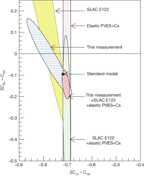
Figure 2: Taken from [58], we see that the parameter space of EW couplings is already constrained by a number of measurements from both atomic physics and electron scattering experiments.

The progress made in such SM tests can be conveniently parametrized in a space spanned by the linear combinations $2C_{1u}-C_{1d}$ vs. $2C_{2u}-C_{2d}$, as illustrated in Fig. 2. The excluded regions of that plot emphasize that much progress has indeed already been made in constraining the parameter space, with the strongest constraints coming from atomic parity violation measurements (specifically, of the weak charge $Q_{W}$ in Cesium [57]) and electron scattering experiments — especially the recent results obtained by the JLab PVDIS Collaboration [58]. For the former, the weak charge of an arbitrary nucleus of $Z$ protons and $N$ neutrons can be determined at tree-level from Eq. (12) to be [59]

$$Q^{Z,N}_{W}\ =\ -2\Big{(}C_{1u}\cdot[2Z+N]+C_{1d}\cdot[Z+2N]\Big{)}\ ;$$ (16)

thus, parity-violating transitions within electron clouds surrounding heavy nuclei (for example, $6S\rightarrow 7S$ in ¹³³Cs) may serve as an alternative means of constraining the parameter space of Fig. 2.

SM tests aside, it has also been suggested more recently that PVDIS can be used to probe parton distribution functions in the largely unmeasured region of high Bjorken-$x$ [60, 61]. In particular, the PVDIS asymmetry for a proton is proportional to the ratio of $d$ to $u$ quark distributions at large $x$. Current determinations of the $d/u$ ratio rely heavily on inclusive proton and deuteron DIS data, and there are large uncertainties in the nuclear corrections in the deuteron at high $x$ [62]. While novel new methods have been suggested to minimize the nuclear uncertainties [63, 64, 65], the use of a proton target alone would avoid the problem altogether.

In this chapter we shall follow the arguments of [66] in order to examine the accuracy of the parton model predictions for the PVDIS asymmetries in realistic experimental kinematics at finite $Q^{2}$. In particular, in Sec. 2 we provide a complete set of formulas for cross sections and asymmetries for scattering polarized leptons from unpolarized targets, including finite-$Q^{2}$ effects. PVDIS from the proton is discussed in Sec. 1, where we test the sensitivity of the extraction of the $d/u$ ratio at large $x$ to finite-$Q^{2}$ corrections. One of the main uncertainties in the calculation is the ratio of longitudinal to transverse cross sections for the $\gamma$–$Z^{0}$ interference, for which no empirical information currently exists, and we provide some numerical estimates of the possible dependence of the left-right asymmetry on this ratio. We also briefly explore in Sec. 2 the possibility of using PVDIS with polarized targets to constrain quark helicity distributions at large $x$. As a comprehensive discussion of polarized PVDIS in the parton model was previously given by Anselmino et al. [67], we here perform a numerical survey of the sensitivity of polarized PVDIS asymmetries to spin-dependent PDFs.

Finally, for deuteron targets, we examine in Sec. 3 how the asymmetry is modified in the presence of finite-$Q^{2}$ corrections, and where these can pose significant backgrounds for extracting standard model signals. In addition, we highlight in Sec. 3 a novel high-energy process on the deuteron based on [68] that may offer a novel degree of sensitivity to quark-level charge symmetry breaking (CSV).

2 Nucleon Structure from Parity-Violation

Kinematically, we again work in the framework of DIS as established in Chap. 1. In this setting, we discuss the general decomposition of the hadronic tensor, and provide formulas for the PV asymmetry in terms of structure functions, and in the parton model in terms of PDFs.

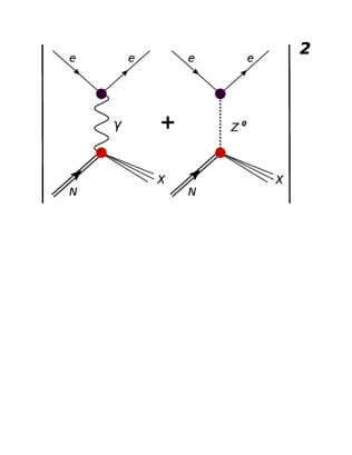
Figure 3: The dominant parity-violating contribution to neutral current DIS derives from the interaction of purely electromagnetic (left diagram) and purely weak amplitudes (right diagram).

Hadronic Tensor.

We begin with the differential cross section for inclusive electron–nucleon scattering, which in general can be written as the squared sum of the $\gamma$- and $Z^{0}$-exchange amplitudes. We will consider contributions to the cross section from the pure $\gamma$ exchange amplitude $A_{\gamma}$ and the $\gamma$–$Z$ interference $A_{\gamma Z}$ as depicted in Fig. 3; the purely weak $Z^{0}$ exchange contribution to the cross section is strongly suppressed relative to these by the weak coupling $G_{F}$ and is therefore not considered in the numerical analysis following these derivations.

Formally, the cross section can be written in terms of products of leptonic and hadronic tensors as [67, 69]:

$$\frac{d^{2}\sigma}{d\Omega dE^{\prime}} ={\alpha^{2}\over Q^{4}}{E^{\prime}\over E}\,\,\bigg{|}\,A_{\gamma}+A_{Z}\,\bigg{|}^{2}\ ,$$

$$={\alpha^{2}\over Q^{4}}{E^{\prime}\over E}\left(L^{\gamma}_{\mu\nu}W^{\mu\nu}_{\gamma}\ +\ {G_{F}\over 4\sqrt{2}\pi\alpha}L^{\gamma Z}_{\mu\nu}W^{\mu\nu}_{\gamma Z}+\ {G^{2}_{F}\over 32\pi^{2}\alpha^{2}}L^{Z}_{\mu\nu}W^{\mu\nu}_{Z}\right)\ ,$$ (17)

where $E$ and $E^{\prime}$ are the (rest frame) electron energies, $Q^{2}$ is (minus) the $4$-momentum transfer squared, and $\alpha$ is the electromagnetic fine structure constant, keeping with the conventions laid out in Chap. 1.1.

Following Eq. (5), the lepton tensor $L^{i}_{\mu\nu}$ encodes the coupling of the scattered electron/neutrino to the exchange boson(s) [i.e., ($i=\gamma,\ \gamma Z,\ Z$)] as [22]

$$L^{\gamma}_{\mu\nu} = 2\left(l_{\mu}l^{\prime}_{\nu}+l^{\prime}_{\mu}l_{\nu}-l\cdot l^{\prime}g_{\mu\nu}+i\lambda\varepsilon_{\mu\nu\alpha\beta}\ l^{\alpha}l^{\prime\beta}\right)\ ,$$

$$L^{\gamma Z}_{\mu\nu} = (g^{e}_{V}+\lambda g^{e}_{A})\ L^{\gamma}_{\mu\nu}\ ,$$

$$L^{Z}_{\mu\nu} = (g^{e}_{V}+\lambda g^{e}_{A})^{2}\ L^{\gamma}_{\mu\nu}\ ,$$

$$L^{W}_{\mu\nu} = (1+\lambda\cdot e)^{2}\ L^{\gamma}_{\mu\nu}\ ,$$ (18)

for leptons of charge $e=\pm 1$ and helicity $\lambda=\pm 1$. Note that the structure of $L^{W}_{\mu\nu}$ prohibits charged current exchanges for positive-helicity electrons or negative-helicity positrons.

The complementary hadronic tensors for the electromagnetic, interference, and weak contributions are then given by:

$$W_{\mu\nu}^{\gamma} = {1\over 2M}\sum_{X}\,\langle X|J_{\mu}^{\gamma}|N\rangle^{*}\langle X|J_{\nu}^{\gamma}|N\rangle\times(2\pi)^{3}\ \delta(k_{X}-p-q)\ ,$$ (19)

$$W_{\mu\nu}^{\gamma Z} = {1\over 2M}\sum_{X}\left\{\langle X|J_{\mu}^{Z}|N\rangle^{*}\langle X|J_{\nu}^{\gamma}|N\rangle+\langle X|J_{\mu}^{\gamma}|N\rangle^{*}\langle X|J_{\nu}^{Z}|N\rangle\right\}\times(2\pi)^{3}\ \delta(k_{X}-p-q)\ ,$$ (20)

$$W_{\mu\nu}^{Z} = {1\over 2M}\sum_{X}\,\langle X|J_{\mu}^{Z}|N\rangle^{*}\langle X|J_{\nu}^{Z}|N\rangle\times(2\pi)^{3}\ \delta(k_{X}-p-q)\ ,$$ (21)

where $M$ is again the nucleon mass, and $J_{\mu}^{\gamma,\gamma Z,Z}$ correspond to the electromagnetic, interference, and weak hadronic current, respectively, cf. Eq. (8). In general, the hadronic tensor for a nucleon with spin $4$-vector $S^{\mu}$ can be written in terms of three spin-independent and five spin-dependent structure functions [67]:

$$W_{\mu\nu}^{i} = -\frac{g_{\mu\nu}}{M}\ F_{1}^{i}\ +\ \frac{p_{\mu}p_{\nu}}{M\ p\cdot q}\ F_{2}^{i}\ +\ \frac{i\varepsilon_{\mu\nu\alpha\beta}p^{\alpha}q^{\beta}}{2Mp\cdot q}\ F_{3}^{i}$$

$$+ \frac{i\varepsilon_{\mu\nu\alpha\beta}}{p\cdot q}\left(q^{\alpha}S^{\beta}\ g_{1}^{i}+2xp^{\alpha}S^{\beta}\ g_{2}^{i}\right)\ -\ \frac{p_{\mu}S_{\nu}+S_{\mu}p_{\nu}}{2p\cdot q}\ g_{3}^{i}+\frac{S\cdot q\ p_{\mu}p_{\nu}}{(p\cdot q)^{2}}\ g_{4}^{i}+\ \frac{S\cdot q\ g_{\mu\nu}}{p\cdot q}\ g_{5}^{i}\ ,$$

for both the electromagnetic ($i=\gamma$) and interference ($i=\gamma Z$) currents. Each of the structure functions generally depend on two variables, usually taken to be $Q^{2}$ and the Bjorken scaling variable $x=Q^{2}/2M\nu$, where $\nu$ is the DIS energy transfer.

Performing the appropriate contractions of $W_{\mu\nu}$ with its leptonic counterpart, we can write a general expression in terms of the structure functions of Eq. (2). Up to kinematical prefactors independent of lepton helicity and target spin (and therefore of no consequence for left-right helicity or spin asymmetries), we have

$$\sigma_{\lambda}={d^{2}\sigma_{\lambda}\over d\Omega dE^{\prime}} =\sum_{\{i=\gamma,\ \gamma Z,\ Z\}}\eta_{i}\ g^{e}_{i}\,\biggl{\{}2xy\,F_{1}^{i}+{2\over y}\left(1-y-{xyM\over 2E}\right)(F_{2}^{i}+g_{3}^{i})-2\lambda x\left(1-{y\over 2}\right)F_{3}^{i}$$

$$-2\lambda x\left(2-y-{xyM\over E}\right)g_{1}^{i}+4\lambda{x^{2}M\over E}\,g_{2}^{i}+{2\over y}\left(1-y-{xyM\over 2E}\right)\,g_{3}^{i}$$

$$-{2\over y}\left(1+{xM\over E}\right)\left(1-y-{xyM\over 2E}\right)g_{4}^{i}+2xy\left(1+{xM\over E}\right)g_{5}^{i}\biggl{\}}\ ,\ \mathrm{and}$$

$$\eta_{\gamma}=1\ ,\ \ \ \eta_{\gamma Z}={G_{F}\over 4\sqrt{2}\pi\alpha}\ ,\ \ \ \eta_{Z}={G^{2}_{F}\over 32\pi^{2}\alpha^{2}}\ ;$$ (23)

for the sake of computing the asymmetry, we let $g^{e}_{\gamma}=1$, $g^{e}_{\gamma Z}=g^{e}_{V}+\lambda g^{e}_{A}$, and $g^{e}_{Z}=(g^{e}_{V}+\lambda g^{e}_{A})^{2}$, after choosing a convenient set of coordinates to treat a longitudinally spin-polarized nucleon target.

Below we will consider scattering of a polarized electron from an unpolarized hadron target, in which only the spin-independent structure functions $F_{1-3}^{\gamma Z}$ enter. Asymmetries resulting from scattering of an unpolarized electron beam from a polarized target, which are sensitive to the spin-dependent structure functions $g_{1-5}^{\gamma Z}$, will be discussed in Sec. 2.

Beam Asymmetries.

The PV interference structure functions can be isolated by constructing an asymmetry between cross sections for right- ($\sigma_{\lambda=+1}$) and left-hand ($\sigma_{\lambda=-1}$) polarized electrons:

$$A^{\rm PV}=\frac{\sigma_{\lambda=+1}-\sigma_{\lambda=-1}}{\sigma_{\lambda=+1}+\sigma_{\lambda=-1}}\ ,$$ (24)

in which $\sigma_{\lambda}\equiv d^{2}\sigma_{\lambda}/d\Omega dE^{\prime}$ as defined in Eq. (23). Since the purely electromagnetic contribution to the cross section is independent of electron helicity, it cancels in the numerator, essentially leaving only the $\gamma$–$Z$ interference term due to the strong suppression of the purely weak process by the squared coupling $G^{2}_{F}$. The denominator, on the other hand, contains all contributions, but is dominated by the purely electromagnetic component. In terms of structure functions, the PVDIS asymmetry may thus be written as

$$A^{\rm PV}=-\left({G_{F}Q^{2}\over 4\sqrt{2}\pi\alpha}\right){g^{e}_{A}\left(2xyF_{1}^{\gamma Z}-2[1-1/y+xM/E]F_{2}^{\gamma Z}\right)+g^{e}_{V}\ x(2-y)F_{3}^{\gamma Z}\over 2xyF_{1}^{\gamma}-2[1-1/y+xM/E]F_{2}^{\gamma}}\ ,$$ (25)

where $y=\nu/E$ is the lepton fractional energy loss.

In the Bjorken limit ($Q^{2},\nu\to\infty$, $x$ fixed), the interference structure functions $F_{1}^{\gamma Z}$ and $F_{2}^{\gamma Z}$ are related by the Callan-Gross relation, $F_{2}^{\gamma Z}=2xF_{1}^{\gamma Z}$, similar to the electromagnetic $F_{1,2}^{\gamma}$ structure functions [67]. This behavior may be encapsulated equivalently by the vanishing of a longitudinal structure function $F^{i}_{L}=F^{i}_{2}-2xF^{i}_{1}$ corresponding to the associated component of Eq. (45). At finite $Q^{2}$, however, corrections to the Callan-Gross relation are usually parametrized in terms of the ratio of the longitudinal to transverse virtual photon cross sections:

$$R^{\gamma(\gamma Z)}\ \equiv\ \frac{\sigma_{L}^{\gamma(\gamma Z)}}{\sigma_{T}^{\gamma(\gamma Z)}}\ =\ r^{2}\frac{F_{2}^{\gamma(\gamma Z)}}{2xF_{1}^{\gamma(\gamma Z)}}-1\ ,$$ (26)

for both the electromagnetic ($\gamma$) and interference ($\gamma Z$) contributions, with

$$r^{2}=1+{Q^{2}\over\nu^{2}}=1+{4M^{2}x^{2}\over Q^{2}}\ .$$ (27)

In terms of this ratio, the PVDIS asymmetry can be written more compactly as:

$$A^{\rm PV}=-\left({G_{F}Q^{2}\over 4\sqrt{2}\pi\alpha}\right)\left[g^{e}_{A}\ Y_{1}\ \frac{F_{1}^{\gamma Z}}{F_{1}^{\gamma}}\ +\ {g^{e}_{V}\over 2}\ Y_{3}\ \frac{F_{3}^{\gamma Z}}{F_{1}^{\gamma}}\right]\ ,$$ (28)

where the functions $Y_{1,3}$ parametrize the dependence on $y$ and on the $R$ ratios:

$$Y_{1} =\frac{1+(1-y)^{2}-y^{2}(1-r^{2}/(1+R^{\gamma Z}))-2xyM/E}{1+(1-y)^{2}-y^{2}(1-r^{2}/(1+R^{\gamma}))-2xyM/E}\left(\frac{1+R^{\gamma Z}}{1+R^{\gamma}}\right)\ ,$$ (29a)

$$Y_{3} =\frac{1-(1-y)^{2}}{1+(1-y)^{2}-y^{2}(1-r^{2}/(1+R^{\gamma}))-2xyM/E}\left(\frac{r^{2}}{1+R^{\gamma}}\right)\ .$$ (29b)

In the Bjorken limit, the kinematical ratio $r^{2}\to 1$, while the longitudinal cross section vanishes relative to the transverse, $R^{i}\to 0$, for both $i=\gamma$ and $\gamma Z$ as we described in Chap. The nonperturbative structure of hadrons. Physically, we are now in a position to correctly interpret this behavior as a feature of asymptotic scattering from pointlike constituent quarks, for which a purely leading twist calculation is an accurate treatment. On the other hand, for kinematics relevant to future experiments ($Q^{2}\sim$ few GeV², $\nu\sim$ few GeV), the factor $2xyM/E$ provides a small correction, and can for practical purposes be dropped. In this case the functions $Y_{1}$ and $Y_{3}$ have the familiar limits [48]:

$$Y_{1} \to 1\ ,$$ (30a)

$$Y_{3} \to\frac{1-(1-y)^{2}}{1+(1-y)^{2}}\ \equiv\ f(y)\ .$$ (30b)

Typically the contribution from the $Y_{3}$ term is much smaller than from the $Y_{1}$ term because $g_{V}^{e}\ll g_{A}^{e}$, although for quantitative comparisons it must be included.

Electroweak Structure Functions.

The PVDIS asymmetry $A^{\rm PV}$ can be evaluated from knowledge of the electromagnetic and interference structure functions. At leading twist, the electroweak structure functions may be expressed in terms of PDFs; for reference these are listed as follows (at leading order in $\alpha_{s}$):

$$\begin{aligned} F_{1}^{\gamma}(x)&=\frac{1}{2}\sum_{q}e_{q}^{2}\ (q(x)+\bar{q}(x))\ ;\\ F_{2}^{\gamma}(x)&=2xF_{1}^{\gamma}(x)\ ;\\ F_{3}^{\gamma}(x)&=0\ ;\end{aligned}\hskip 22.76228pt\vspace*{0.2cm}\begin{aligned} \vspace*{0.2cm}F_{1}^{\gamma Z}(x)&=\sum_{q}e_{q}\ g_{V}^{q}\ (q(x)+\bar{q}(x))\ ;\\ F_{2}^{\gamma Z}(x)&=2xF_{1}^{\gamma Z}(x)\ ;\\ F_{3}^{\gamma Z}(x)&=2\sum_{q}e_{q}\ g_{A}^{q}\ (q(x)-\bar{q}(x))\ ;\end{aligned}$$ (31)

in Eq. (31) the quark $q$ and antiquark $\bar{q}$ distributions are defined with respect to the proton.

For the sake of completeness, we note the weak neutral collection using our conventions to be

$$F_{1}^{Z}(x) =\frac{1}{2}\sum_{q}(g^{q\,2}_{A}+g^{q\,2}_{V})\ (q(x)+\bar{q}(x))\ ,$$ (32a)

$$F_{2}^{Z}(x) =2xF_{1}^{Z}(x)\ ,$$ (32b)

$$F_{3}^{Z}(x) =2\sum_{q}g_{A}^{q}\ g_{V}^{q}\ (q(x)-\bar{q}(x))\ .$$ (32c)

In terms of PDFs, the PV asymmetry in Eq. (28) can be neatly written as:

$$A^{\rm PV}=-\left({G_{F}Q^{2}\over 4\sqrt{2}\pi\alpha}\right)\left(Y_{1}\ a_{1}\ +\ Y_{3}\ a_{3}\right)\ ,$$ (33)

with the hadronic vector and axial-vector terms being respectively given by

$$a_{1}=\frac{2\sum_{q}e_{q}\ C_{1q}\ (q+\bar{q})}{\sum_{q}e_{q}^{2}\ (q+\bar{q})}\ ;\hskip 28.45274pta_{3}=\frac{2\sum_{q}e_{q}\ C_{2q}\ (q-\bar{q})}{\sum_{q}e_{q}^{2}\ (q+\bar{q})}\ .$$ (34)

In this analysis we will focus on the large-$x$ region dominated by valence quarks, so that the effects of sea quark will be negligible.

At finite $Q^{2}$, corrections to the parton model expressions appear in the form of perturbatively generated $\alpha_{s}$ corrections, target mass corrections [44], as well as higher twist ($1/Q^{2}$ suppressed) effects. Some of these effects have been tentatively investigated in the literature [70], and in Chap. 3 we consider the issue of TMCs, but in the present chapter we focus on the finite-$Q^{2}$ effects on the asymmetry arising from non-zero values of $R^{\gamma(\gamma Z)}$, which to date have not been systematically considered. While data and phenomenological parameterizations are available for $R^{\gamma}$ [72, 73, 74], currently no empirical information exists on $R^{\gamma Z}$. In our numerical estimates below, we shall consider a range of possible behaviors for $R^{\gamma Z}$ and examine its effect on $A^{\rm PV}$.

1 PVDIS on the Proton

Parity-violating DIS on a proton target has recently been discussed as a means of constraining the ratio of $d$ to $u$ quark distributions at large $x$ [60] — a quantity that has the means of differentiating among various quark models of the nucleon’s valence structure. At present the $d/u$ ratio is essentially unknown beyond $x\sim 0.6$ due to large uncertainties in the nuclear corrections in the deuteron, which is the main source of information on the $d$ quark distribution [62, 65]. Several new approaches to determining $d/u$ at large $x$ have been proposed, for example using spectator proton tagging in semi-inclusive DIS from the deuteron [64] (similar to the process analyzed in Chap. 5), or through a ratio of ³He and ³H targets to cancel the nuclear corrections [63]. The virtue of the PVDIS method is that, rather than using different hadrons (or nuclei) to select different flavors, here one uses [the interference of] different gauge bosons to act as a flavor “filter,” thereby avoiding nuclear uncertainties altogether.

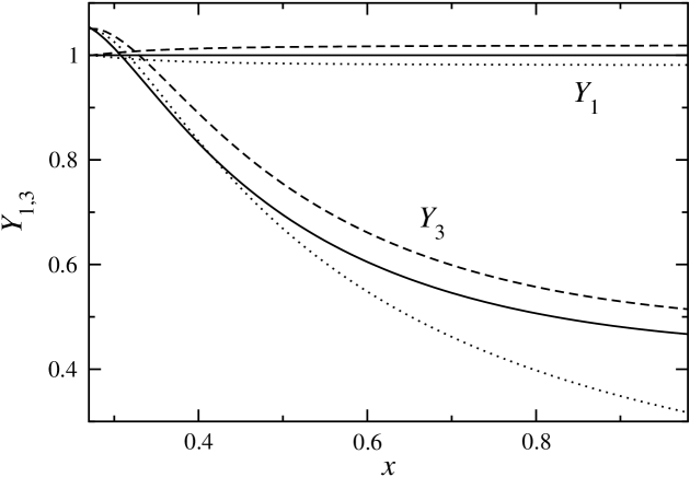
Figure 4: $Y_{1}$ and $Y_{3}$ as a function of $x$, for $Q^{2}=5$ GeV² and $E=10$ GeV. For $Y_{1}$, the solid line (at $Y_{1}=1$) corresponds to $R^{\gamma Z}=R^{\gamma}$ [72], while the dotted lines correspond to $\pm 20\%$ deviations of $R^{\gamma Z}$ from $R^{\gamma}$. For $Y_{3}$, the Bjorken limit result ($R^{\gamma}=0,r^{2}=1$) is given by the dotted curve, the dashed has $R^{\gamma}=0$ but $r^{2}\neq 1$, while the solid represents the full result.

In the valence region at large $x$, the PV asymmetry is sensitive to the valence $u$ and $d$ quark distributions in the proton. Here the functions $a_{1}$ and $a_{3}$ in Eqs. (34) for the proton can be simplified to:

$$a_{1}^{p}=\frac{12C_{1u}-6C_{1d}\ d/u}{4+d/u}\ ,$$ (35a)

and

$$a_{3}^{p}=\frac{12C_{2u}-6C_{2d}\ d/u}{4+d/u}\ .$$ (35b)

This reveals that both $a_{1}^{p}$ and $a_{3}^{p}$ depend directly on the $d/u$ quark distribution ratio.

To explore the relative sensitivity of the proton asymmetry $A^{\rm PV}_{p}$ to the vector and axial vector terms, in Fig. 4 we show the functions $Y_{1}$ and $Y_{3}$ for the proton as a function of $x$, evaluated at $Q^{2}=5$ GeV², for a beam energy $E=10$ GeV (which we will assume throughout). For $Y_{1}$, the solid line (at $Y_{1}=1$) corresponds to $R^{\gamma Z}=R^{\gamma}$, while the dashed (dotted) curves around it represent $+(-)20\%$ deviations of $R^{\gamma Z}$ from $R^{\gamma}$. For $Y_{3}$, the Bjorken limit result ($R^{\gamma}=0,r^{2}=1$) is given by the dotted curve, the dashed curve has $R^{\gamma}=0$ but $r^{2}\neq 1$, while the solid represents the full result with $R^{\gamma}\neq 0$ and $r^{2}\neq 1$. In all cases we use $R^{\gamma}$ from the parameterization of Ref. [72]. The results with the parameterization of Ref. [73] are very similar, and are consistent within the quoted uncertainties.

Note that at fixed $Q^{2}$, the large-$x$ region also corresponds to low hadronic final state masses $W$, so that with increasing $x$ one eventually encounters the resonance region at $W\lesssim 2$ GeV (akin to the behavior illustrated for exclusive photoproduction in Fig. 5 of Chap. 1.2). For $Q^{2}=5$ GeV² this occurs at $x\approx 0.62$, and for $Q^{2}=10$ GeV² at $x\approx 0.76$. This may introduce an additional source of uncertainty in the extraction of the PV asymmetry at large $x$, arising from possible higher twist corrections to structure functions. In actual experimental conditions, the value of $Q^{2}$ can be varied with $x$ to ensure that the resonance region is excluded from the data analysis. For the purposes of illustrating the finite-$Q^{2}$ effects in our analysis, we shall fix $Q^{2}$ at the low end of values attainable with an energy of $E=10$ GeV, namely $Q^{2}=5$ GeV².

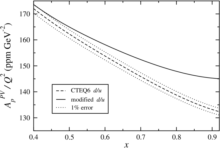
Figure 5: Proton PV asymmetry $A^{\rm PV}_{p}/Q^{2}$ as a function of $x$, for $Q^{2}=5$ GeV², in parts per million (ppm) $\cdot$ GeV^-2. The prediction with the standard CTEQ6 PDFs (dashed) is compared with that using a modified $d/u$ ratio at large $x$ (solid). A $\pm 1\%$ uncertainty band (dotted) is shown around the standard CTEQ6 prediction.

The sensitivity of the proton asymmetry $A^{\rm PV}_{p}$, measured in parts per million (ppm), to the $d/u$ ratio is illustrated in Fig. 5 as a function of $x$, for $Q^{2}=5$ GeV², where $A^{\rm PV}_{p}/Q^{2}$ is shown. Here we assume that $R^{\gamma Z}=R^{\gamma}$, so that the coefficient $Y_{1}$ in the vector term is unity. For the $u$ and $d$ distributions we use the CTEQ6 PDF set [75], in which the $d/u$ ratio vanishes as $x\to 1$, along with a modified $d/u$ ratio which has a finite $x\to 1$ limit of 0.2 [62], $d/u\to d/u+0.2\ x^{2}\ \exp(-(1-x)^{2})$ [76], motivated by theoretical counting rule arguments [77]. Also shown (dotted band around the CTEQ6 prediction) is a $\pm 1\%$ uncertainty, which is a conservative estimate of what may be expected experimentally at JLab with 12 GeV [60, 51]. The results indicate that a signal for a larger $d/u$ ratio would be clearly visible above the experimental errors.

At finite $Q^{2}$ the asymmetry $A^{\rm PV}_{p}$ depends not only on the PDFs, but also on the longitudinal to transverse cross sections ratios $R^{\gamma}$ and $R^{\gamma Z}$ for the electromagnetic and $\gamma Z$ interference contributions, respectively. A number of measurements of the former have been taken at SLAC and JLab [72, 73, 74], and parameterizations of $R^{\gamma}$ in the DIS region exist. As such, the contribution from $R^{\gamma}$ is under comparatively better control, both theoretically and experimentally.

These effects are to be compared with the relative change in $A^{\rm PV}_{p}$ arising from different large-$x$ behaviors of the $d/u$ ratio (dashed curve), expressed as a difference of the asymmetries with the standard CTEQ6 [75] PDFs and ones with a modified $d/u$ ratio [62, 76], $\delta^{(d/u)}A_{p}^{\rm PV}/A_{p}^{\rm PV(0)}$. where $A_{p}^{\rm PV(0)}$ is computed in terms of the standard (unmodified) PDFs. This is of the order 2% for $x\sim 0.5$, but rises rapidly to $\sim 10\%$ for $x\sim 0.9$. While the kinematical and $R^{\gamma}$ corrections are smaller than the (maximal) $d/u$ effect on the asymmetry, these must be included in the data analysis in order to minimize the uncertainties on the extracted $d/u$ ratio.

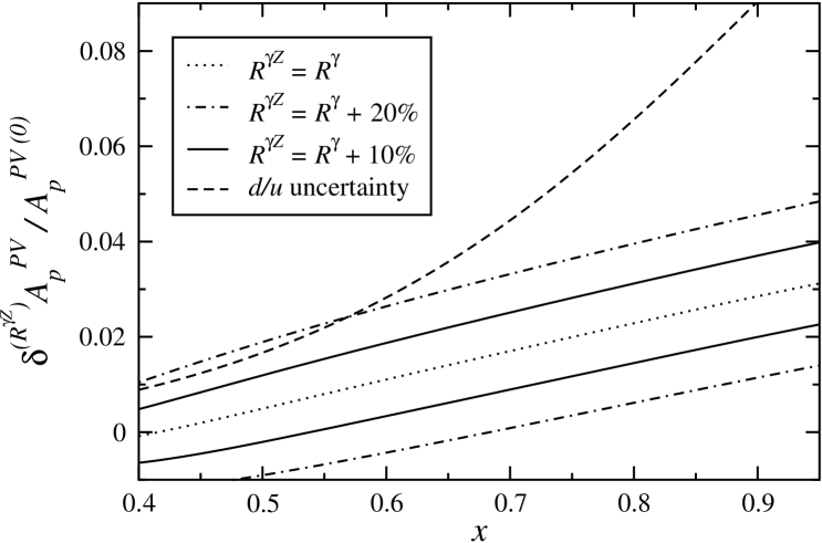
Figure 6: Relative effects on the proton PV asymmetry $A^{\rm PV}_{p}$ from the $\gamma Z$ interference ratio $R^{\gamma Z}$ compared with the Bjorken limit asymmetry $A^{\rm PV\ (0)}_{p}$. The baseline result for $R^{\gamma Z}=R^{\gamma}$ (dotted) is compared with the effects of modifying $R^{\gamma Z}$ by $\pm 10\%$ (solid) and $\pm 20\%$ (dot-dashed), for $Q^{2}=5$ GeV². For reference the relative uncertainty $\delta^{(d/u)}A_{p}^{\rm PV}/A_{p}^{\rm PV(0)}$ from the $d/u$ ratio is also shown (dashed).

In contrast to $R^{\gamma}$, no experimental information currently exists on the interference ratio $R^{\gamma Z}$. Since $R^{\gamma Z}$ enters in the relatively large $Y_{1}$ contribution to $A^{\rm PV}_{p}$, any differences between $R^{\gamma Z}$ and $R^{\gamma}$ could have important consequences for the asymmetry. At high $Q^{2}$ one expects that $R^{\gamma Z}\approx R^{\gamma}$ at leading twist, if the PVDIS process is dominated by single quark scattering. At low $Q^{2}$, however, since the current conservation constraints are different for weak and electromagnetic probes, there may be significant differences between these [78].

To explore the potential effects of $R^{\gamma Z}$ on $A^{\rm PV}_{p}$ we therefore consider several possible scenarios for the ratios. These are illustrated in Fig. 6, where we plot the ratio $\delta^{(R^{\gamma Z})}A^{\rm PV}_{p}/A^{\rm PV(0)}_{p}$, where $\delta^{(R^{\gamma Z})}A^{\rm PV}_{p}$ is the difference between the full asymmetry and that calculated in Bjorken limit kinematics, $A^{\rm PV(0)}_{p}$. The baseline correction with $R^{\gamma Z}=R^{\gamma}$ (dotted curve), with $R^{\gamma}$ from Ref. [72], is compared with the effects of modifying $R^{\gamma Z}$ by $\pm 10\%$ (solid) and $\pm 20\%$ (dot-dashed). The result of such a modification, which comes through the $Y_{1}$ term in the asymmetry, is an $\approx$ 1% (2%) shift of $A^{\rm PV}_{p}$ relative to the $R^{\gamma Z}$-independent asymmetry. For $x\lesssim 0.6$, a 20% difference between $R^{\gamma Z}$ and $R^{\gamma}$ would be comparable to, or exceed, the maximal $d/u$ uncertainty considered here (dashed curve), although at larger $x$ the sensitivity of $A^{\rm PV}_{p}$ to $d/u$ becomes increasingly stronger. As with the $R^{\gamma}$ corrections discussed at length in [66], the possible effects on the asymmetry due to $R^{\gamma Z}$ are potentially significant, which partially motivates work in subsequent chapters (esp., Chap. 3) to estimate possible differences with $R^{\gamma}$.

2 Spin-Polarized PVDIS

In this section we explore the possibility of extracting spin-dependent PDFs in parity-violating unpolarized-electron scattering from a polarized hadron. In particular, we examine the sensitivity of the polarized proton, neutron and deuteron PVDIS asymmetries to the polarized $\Delta u$ and $\Delta d$ distributions at large $x$, where these are poorly known. The $\Delta d$ distribution in particular remains essentially unknown beyond $x\approx 0.6$.

Using Eq. (23), the PV differential cross-section (with respect to the variables $x$ and $y$) for unpolarized electrons on longitudinally polarized nucleons can generally be written in terms of five spin-dependent structure functions [67]:

$$\frac{d^{2}\sigma^{\rm PV}}{dxdy}(\bar{\lambda},S_{L}) = 2x\left(2-y-\frac{xyM}{E}\right)g_{1}^{\gamma Z}\ -\ \frac{4x^{2}M}{E}\ g_{2}^{\gamma Z}\ +\ \frac{2}{y}\left(1-y-\frac{xyM}{2E}\right)g_{3}^{\gamma Z}$$ (36)

$$-\ \frac{2}{y}\left(1+\frac{xM}{E}\right)\left(1-y-\frac{xyM}{2E}\right)g_{4}^{\gamma Z}\ +\ 2xy\left(1+\frac{xM}{E}\right)g_{5}^{\gamma Z}\ ,$$

where the nucleon (longitudinal) spin vector $S_{L}$ is given by $S^{\mu}_{L}=(0;0,0,1)$, and $\bar{\lambda}$ is the average over $\lambda=+1$ and $\lambda=-1$ [see Eq. (23)]. The analogue of the PV asymmetry in Eq. (24) for a polarized target can be defined as:

$$\Delta A^{\rm PV}=\frac{\sigma^{\rm PV}(\bar{\lambda},S_{L})-\sigma^{\rm PV}(\bar{\lambda},-S_{L})}{\sigma^{\rm PV}(\bar{\lambda},S_{L})+\sigma^{\rm PV}(\bar{\lambda},-S_{L})}\ ,$$ (37)

where $\sigma^{\rm PV}(\bar{\lambda},S_{L})\equiv d^{2}\sigma^{\rm PV}/dxdy$. Some of the structure functions $g_{1-5}^{\gamma Z}$ have simple parton model interpretations, whereas others do not; either way, at present there is essentially no phenomenological information about them. In order to proceed, we shall therefore consider the asymmetry in the high energy limit, $M/E\to 0$, which eliminates the structure function $g_{2}^{\gamma Z}$. In this limit, the operator product expansion gives rise to the relation $g_{3}^{\gamma Z}-g_{4}^{\gamma Z}=2xg_{5}^{\gamma Z}$, which further eliminates one of the functions. Furthermore, in the parton model the $g_{4}^{\gamma Z}$ structure function vanishes, leaving the Callan-Gross-like relation $g_{3}^{\gamma Z}=2xg_{5}^{\gamma Z}$. In terms of the remaining two structure functions, the spin-dependent PV asymmetry may be written:

$$\Delta A^{\rm PV}=\frac{G_{F}Q^{2}}{4\sqrt{2}\pi\alpha}\left(g_{A}^{e}\ f(y)\ \frac{g_{1}^{\gamma Z}}{F_{1}^{\gamma}}\ +\ g_{V}^{e}\ \frac{g_{5}^{\gamma Z}}{F_{1}^{\gamma}}\right)\ ,$$ (38)

where the kinematical factor $f(y)$ is given in Eq. (30b).

As an aside we note that the clean isolation of such spin-polarized observables could present yet another opportunity to test the predictions and structure of QCD and the SM; this is evident by the form of spin-polarized sum rules analogous to the relations mentioned in Eqs. (5a & 5b), which may be derivable in the QPM in terms of quark-level quantities and electroweak parameters. For example, this is the case with the electromagnetic Bjorken sum rule [84],

$$S_{B}\ =\ \int_{0}^{1}\ dx\left\{g^{\gamma}_{1p}(x,Q^{2})\ -\ g^{\gamma}_{1n}(x,Q^{2})\right\}\ ={g_{A}\over 6}+\mathrm{O}(\alpha_{s})\ ,$$ (39)

where $g_{A}\sim 1.26$ is the axial charge of the nucleon predictable by the Adler-Weisberger relation.

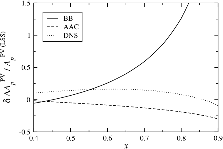
Figure 7: Sensitivity of the polarized proton PV asymmetry $\Delta A^{\rm PV}_{p}$ on the spin-dependent $\Delta u$ and $\Delta d$ distributions. The asymmetries for the BB [85] (solid), AAC [86] (dashed) and DNS [87] (dotted) distributions are evaluated relative to the baseline asymmetry for the LSS PDFs [88].

In the QCD parton model the $g_{1}^{\gamma Z}$ and $g_{5}^{\gamma Z}$ structure functions can be expressed in terms of helicity dependent PDFs $\Delta q$ as [67]:

$$g_{1}^{\gamma Z} = \sum_{q}e_{q}\ g_{V}^{q}\left(\Delta q+\Delta\bar{q}\right)\ ,$$ (40a)

$$g_{5}^{\gamma Z} = \sum_{q}e_{q}\ g_{A}^{q}\ \left(\Delta q-\Delta\bar{q}\right)\ ,$$ (40b)

where $\Delta q$ is a function of $x$ and $Q^{2}$. Using these expressions, the PV asymmetries for proton, neutron and deuteron (which in this analysis we take to be a sum of proton and neutron) targets can then be written [83]:

$$\Delta A^{\rm PV}_{p} = \frac{6\ G_{F}Q^{2}}{4\sqrt{2}\pi\alpha}\left[(2C_{1u}\Delta u-C_{1d}\Delta d)f(y)+(2C_{2u}\Delta u-C_{2d}\Delta d)\right]\left({1\over 4u+d}\right)\ ,$$ (41a)

$$\Delta A^{\rm PV}_{n} = \frac{6\ G_{F}Q^{2}}{4\sqrt{2}\pi\alpha}\left[(2C_{1u}\Delta d-C_{1d}\Delta u)f(y)+(2C_{2u}\Delta d-C_{2d}\Delta u)\right]\left({1\over u+4d}\right)\ ,$$ (41b)

$$\Delta A^{\rm PV}_{d} = \frac{3\ G_{F}Q^{2}}{10\sqrt{2}\pi\alpha}\left[(2C_{1u}-C_{1d})f(y)+2C_{2u}-C_{2d}\right]\left({\Delta u+\Delta d\over u+d}\right)\ .$$ (41c)

In Fig. 7 we illustrate the sensitivity of the proton asymmetry $\Delta A^{\rm PV}_{p}$ to the $\Delta u$ and $\Delta d$ PDFs, by comparing the difference $\delta\Delta A^{\rm PV}_{p}$ in the asymmetry arising from different parameterizations [85, 86, 87], relative to the LSS parameterization [88]. The spread among these various schemes reflects varying model assumptions that determine the initial input parametrizations, which are in turn constrained by the limited available data. The resulting effects in $\Delta A^{\rm PV}_{p}$ at intermediate $x$, $x\sim 0.5$–0.6, are of order 20%; however, these increase rapidly with $x$. At $x\approx 0.7$–0.8 the AAC [86], DNS [87] and LSS [88] parameterizations give asymmetries that are within $\sim 20\%$ of each other, whereas the BB fit [85] deviates by 50–100% in this range — a consequence of the lack of precise experimental constraints, especially at high $x$. The results for neutron and deuteron targets are found to be very similar to those in Fig. 7. While this does not constitute a systematic error on the uncertainty in $\Delta A^{\rm PV}_{p}$ due to PDFs, it does indicate the sensitivity of polarized PVDIS to helicity distributions at large $x$, and suggests that a measurement of $\Delta A^{\rm PV}_{p}$ at the 10–20% level could discriminate between different PDF behaviors.

Finally, for completeness we indicate that in principle it should be possible to extract data on the PDF quantities $\Delta u/u$ and $\Delta d/d$ from polarized asymmetries given knowledge of the unpolarized PDF behavior and experimental values for the DIS couplings.

Making the appropriate combinations of single-nucleon polarized asymmetries, we obtain:

$$\frac{\Delta u}{u} = \frac{\sqrt{8}\pi\alpha}{3G_{F}Q^{2}}\cdot{\left(2(C_{1u}f(y)+C_{2u})(4+d/u)\Delta A^{PV}_{p}+(C_{1d}+C_{2d})(4d/u+1)\Delta A^{PV}_{n}\right)\over 4[C_{1u}f(y)+C_{2u}]^{2}+[C_{1d}f(y)+C_{2d}]^{2}}\ ,$$

$$\frac{\Delta d}{d} = \frac{\sqrt{8}\pi\alpha}{3G_{F}Q^{2}}\cdot\frac{[2(C_{1u}f(y)+C_{2u})(4+u/d)\Delta A^{PV}_{n}+(C_{1d}+C_{2d})(4u/d+1)\Delta A^{PV}_{p}]}{4[C_{1u}f(y)+C_{2u}]^{2}+[C_{1d}f(y)+C_{2d}]^{2}}\ .$$

Alternatively, we may write these in terms of the proton and deuteron asymmetries:

$$\frac{\Delta u}{u} = \frac{\sqrt{8}\pi\alpha[(4+d/u)C_{1}(y)\Delta A^{PV}_{p}+5(1+d/u)[C_{1d}f(y)+C_{2d}]\Delta A^{PV}_{d}]}{3G_{F}Q^{2}(C_{1}(y)\cdot C_{2}(y)}\ ,$$ (43a)

$$\frac{\Delta d}{d} = \left(\sqrt{8}\pi\alpha[\frac{5(u/d+1)\Delta A^{PV}_{d}}{C_{1}(y)}-\frac{(4u/d+1)\Delta A^{PV}_{p}}{C_{1u}f(y)+C_{2u}}\right)\Bigg{/}\left(1+\frac{C_{1d}f(y)+C_{2d}}{2(C_{1u}f(y)+C_{2u})}\right)\ .$$

Thus, with precise measurements of $\Delta A^{PV}_{p},\,\Delta A^{PV}_{n},$ and $\Delta A^{PV}_{d}$ the light quark polarizations might be better constrained — a fact that urges further acquisition of spin-polarized DIS asymmetry measurements, particularly at high $x$.

3 Scattering from the Isoscalar Deuteron

For parity-violating scattering from an isoscalar deuteron, the dependence of the left-right asymmetry on PDFs cancels in the parton model, so that the asymmetry is determined entirely by the weak mixing angle, $\theta_{W}$. The deuteron asymmetry is therefore a sensitive test of effects beyond the parton model, such as higher twist contributions, or of more exotic effects such as charge symmetry violation in PDFs or new physics beyond the SM.

In fact as early as the late 1970s parity-violating DIS on the deuteron provided important early tests of the SM [48, 49]. In the parton model, the asymmetry for an isoscalar deuteron becomes independent of hadronic structure, and is therefore given entirely by electroweak coupling constants. At finite $Q^{2}$, however, contributions from longitudinal structure functions, or from higher twist effects, may play a role. The higher twists have been estimated in several phenomenological model studies [70], while more recently, it has been suggested that PVDIS on a deuteron could also be sensitive to charge symmetry violation (CSV) effects in PDFs (see Ref. [71] for a review of CSV in PDFs). In this section we explore the contributions from kinematical finite-$Q^{2}$ effects and the longitudinal structure functions $F^{i}_{L}$ on the PV asymmetry, and assess their impact on the extraction of CSV effects. Having done so, we outline a possible measurement at higher $Q^{2}$ which would be ideally suited to an envisioned electron-ion collider and may well yield an unambiguous CSV signal.

1 Electroweak Structure

Assuming the deuteron is composed of a proton and a neutron, and neglecting possible differences between free and bound nucleon PDFs, the functions $a_{1}$ and $a_{3}$ in Eq. (34) for a deuteron target become:

$$a_{1}^{d} = \frac{6}{5}\left(2C_{1u}-C_{1d}\right)\ ,$$ (44a)

$$a_{3}^{d} = \frac{6}{5}\left(2C_{2u}-C_{2d}\right)\ .$$ (44b)

If in addition $R^{\gamma}_{d}\approx R^{\gamma}_{p}$ and $R^{\gamma Z}_{d}\approx R^{\gamma Z}_{p}$, as is observed experimentally [72], then the $y$-dependent terms in the deuteron asymmetry become $Y_{1}^{d}\approx Y_{1}^{p}\equiv Y_{1}$ and $Y_{3}^{d}\approx Y_{3}^{p}\equiv Y_{3}$. The PV asymmetry can then be written as:

$$A^{\rm PV}=-\left(\frac{3G_{F}Q^{2}}{10\sqrt{2}\pi\alpha}\right)\left[Y_{1}\left(2C_{1u}-C_{1d}\right)\ +\ Y_{3}\left(2C_{2u}-C_{2d}\right)\ \right]\ ,$$ (45)

which in the Bjorken limit ($Y_{1}\to 1$, $Y_{3}\to f(y)$) becomes independent of hadron structure, and is a direct measure of the electroweak coefficients $C_{iq}$.

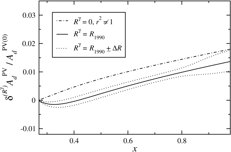
Figure 8: Relative effects on the deuteron PV asymmetry $A^{\rm PV}_{d}$ from the electromagnetic ratio $R^{\gamma}$ (with $R^{\gamma Z}=R^{\gamma}$), compared with the Bjorken limit asymmetry $A^{\rm PV\ (0)}_{d}$. The full results (solid), for $Q^{2}=5$ GeV², are compared with those for $R^{\gamma}=0$ (but $r^{2}\neq 1$) (dot-dashed), with the dotted curves representing the uncertainty on $R^{\gamma}$ from Ref. [72].

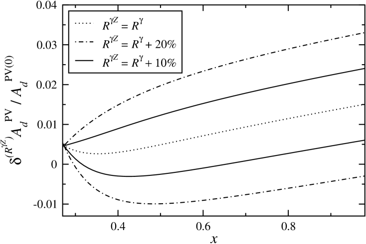
Figure 9: Relative effects on the deuteron PV asymmetry $A^{\rm PV}_{d}$ from the $\gamma Z$ interference ratio $R^{\gamma Z}$ compared with the Bjorken limit asymmetry $A^{\rm PV\ (0)}_{d}$. The baseline result for $R^{\gamma Z}=R^{\gamma}$ (dotted) is compared with the effects of modifying $R^{\gamma Z}$ by $\pm 10\%$ (solid) and $\pm 20\%$ (dot-dashed), for $Q^{2}=5$ GeV².

In Fig. 8 the relative effect on $A^{\rm PV}_{d}$ from $R^{\gamma}$ is shown via the ratio $\delta^{(R^{\gamma})}A^{\rm PV}_{d}/A^{\rm PV(0)}_{d}$, where $\delta^{(R^{\gamma})}A^{\rm PV}_{d}$ is the difference between the full asymmetry and that calculated in Bjorken limit kinematics, $A^{\rm PV(0)}_{d}$. The correction due to $R^{\gamma}$ is comparatively smaller in the deuteron. The effect on $A^{\rm PV}_{d}$ from the purely kinematical $r^{2}$ correction in the $Y_{3}$ term (with $R^{\gamma}=0$) is an increase of order $1\%$ over the Bjorken limit asymmetry in the range $0.5\lesssim x\lesssim 0.9$. Inclusion of the $R^{\gamma}$ ratio cancels the correction somewhat, reducing it to $\lesssim 0$–0.5% for $x\lesssim 0.6$, and to $\lesssim 0.5$–1% for $x>0.6$.

The effects of a possible difference between $R^{\gamma Z}$ and $R^{\gamma}$ are illustrated in Fig. 9 through the ratio $\delta^{(R^{\gamma Z})}A^{\rm PV}_{d}/A^{\rm PV(0)}_{d}$, where $\delta^{(R^{\gamma Z})}A^{\rm PV}_{p}$ is the difference between the full and Bjorken limit asymmetries. As for the proton in Fig. 6, the baseline correction with $R^{\gamma Z}=R^{\gamma}$ (dotted curve, equivalent to the solid curve in Fig. 8) is compared with the effects of modifying $R^{\gamma Z}$ by a constant $\pm 10\%$ (solid) and $\pm 20\%$ (dot-dashed). This results in an additional $\approx$ 1% (2%) shift of $A^{\rm PV}_{d}$ for a 10% (20%) modification relative to the baseline asymmetry for $x>0.5$. Such effects will need to be accounted for if one wishes to compare with SM predictions, or when extracting CSV effects in PDFs, which we discuss in the next subsection.

2 Charge Symmetry Violation

Aside from these general considerations regarding sub-leading $Q^{2}$ corrections to helicity asymmetry measurements from them, scattering from deuteron targets represents a fertile testing ground for the violation of partonic charge symmetry. By definition, charge symmetry is a precise operation involving isospin, which governs the interchange of protons and neutrons, or equivalently, of up and down quarks. The charge symmetry operator ${P_{CS}}$ corresponds to a rotation of $180^{\circ}$ about the $2$ axis in isospin space, such that

$${P_{CS}} =e^{i\pi T_{2}}\ ,$$

$${P_{CS}}|u\rangle =-|d\rangle;\hskip 17.07182pt{P_{CS}}|d\rangle=|u\rangle\ .$$ (46)

It is of particular importance because at low energies, where it has been studied extensively, charge symmetry is a far better symmetry than isospin in general, typically being respected to better than 1% [89, 90, 91]. It is therefore natural to assume that charge symmetry is also valid at the partonic level and, indeed, almost all analyses of parton distribution functions (PDFs) assume charge symmetry, whether the assumption is stated or not. The importance of charge symmetry violation in PDFs within the context of tests of the Standard Model has recently been of considerable interest [92, 93].

In the discussion above an implicit assumption has been made that charge symmetry is exact — namely, that the quark distributions in the proton and neutron are related by $u^{p}=d^{n}$ and $u^{n}=d^{p}$. Quark mass differences and electromagnetic effects are expected, however, to give rise to small violations of charge symmetry in PDFs, which may be parametrized by:

$$\delta u = u^{p}-d^{n}\ ,$$ (47a)

$$\delta d = d^{p}-u^{n}\ .$$ (47b)

Non-zero values of $\delta u$ and $\delta d$ have been predicted in nonperturbative models of the nucleon [79], and can in addition arise from radiative QED effects in $Q^{2}$ evolution [80, 81, 82].

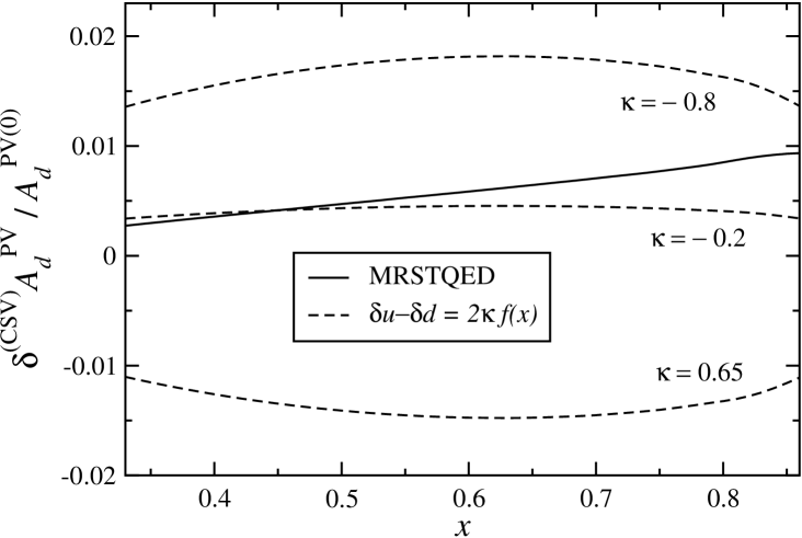
Figure 10: Relative effects on the deuteron PV asymmetry $A^{\rm PV}_{d}$ of CSV in PDFs, compared with the charge symmetric asymmetry. The CSV distributions $\delta u-\delta d$ are from the MRSTQED fit [81] (solid) and from the parameterization $\delta u-\delta d=2\kappa f(x)$ (dashed, see text), with $\kappa=-0.2$ (best fit), and the two 90% confidence levels, $\kappa=-0.8$ and $\kappa=+0.65$ [80].

It is convenient to define the $u$ and $d$ quark distributions in the presence of CSV according to [83]:

$$u\ \equiv\ u^{p}-\frac{\delta u}{2} = d^{n}+\frac{\delta u}{2}\ ,$$ (48a)

$$d\ \equiv\ d^{p}-\frac{\delta d}{2} = u^{n}+\frac{\delta d}{2}\ .$$ (48b)

With these definitions, the deuteron functions $a_{1}^{d}$ and $a_{3}^{d}$ in the $A_{d}^{\rm PV}$ asymmetry can be written:

$$a_{1}^{d} = a_{1}^{d(0)}+\delta^{\rm(CSV)}a_{1}^{d}\ ,$$ (49a)

$$a_{3}^{d} = a_{3}^{d(0)}+\delta^{\rm(CSV)}a_{3}^{d}\ ,$$ (49b)

where $a_{1}^{d(0)}$ and $a_{3}^{d(0)}$ are given by Eqs. (44a) and (44b), respectively. The fractional CSV corrections are then given by:

$$\frac{\delta^{\rm(CSV)}a_{1}^{d}}{a_{1}^{d(0)}} = \left(-\frac{3}{10}+\frac{2C_{1u}+C_{1d}}{2(2C_{1u}-C_{1d})}\right)\left(\frac{\delta u-\delta d}{u+d}\right)\ ,$$ (50a)

$$\frac{\delta^{\rm(CSV)}a_{3}^{d}}{a_{3}^{d(0)}} = \left(-\frac{3}{10}+\frac{2C_{2u}+C_{2d}}{2(2C_{2u}-C_{2d})}\right)\left(\frac{\delta u-\delta d}{u+d}\right)\ .$$ (50b)

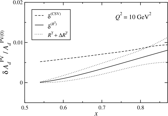
Figure 11: Relative effects on the deuteron PV asymmetry $A^{\rm PV}_{d}$ from CSV in PDFs [80] (dashed, see Fig. 10) and from $R^{\gamma}$ [72] (with $R^{\gamma Z}=R^{\gamma}$, solid) at $Q^{2}=10$ GeV², compared with the charge symmetric asymmetry in Bjorken limit kinematics. The shaded area represents the uncertainty in $R^{\gamma}$.

Using these definitions, we plot in Fig. 10 the effect of CSV in valence PDFs on the deuteron asymmetry $A_{d}^{\rm PV}$. The asymmetry using the MRSTQED paramterization [81] of $\delta u-\delta d$ (solid curve) gives an $\approx 0.5$–1% effect for $0.5\lesssim x\lesssim 0.9$, similar to the effect predicted from nonperturbative (e.g., bag model) calculations [79]. In this case, the constraint to $\delta u-\delta d$ follows from a QCD global fit that explicitly incorporates QED corrections due to finite photon distribution functions $\gamma_{p}(x,Q^{2})\neq\gamma_{n}(x,Q^{2})$. Alternatively, and more directly, MRST also performed a comparable estimate by means of the phenomenological fit [80]

$$\delta u-\delta d\ =\ 2\kappa\cdot f(x)\ ,$$

$$f(x)\ =\ x^{-1/2}(1-x)^{4}(x-0.0909)\ ,$$ (51)

where $\kappa$ is a free parameter; this resulted in a similar correction to the asymmetry, $\sim 0.5\%$ for most of the $x$ range considered. The best fit gives $\kappa=-0.2$, although the constraints on $\kappa$ are relatively weak, with values of $\kappa=-0.8$ and $+0.65$ giving $\sim 1.5$–2% effect for $0.5\lesssim x\lesssim 0.8$ at the 90% confidence level.

For the central values (best fit parameters), the magnitude of the CSV effect on the asymmetry at $Q^{2}=5$ GeV² is similar to that due to the finite-$Q^{2}$ kinematics ($r^{2}\neq 1$, $R^{\gamma}\neq 0$) seen in Fig. 8, and may be smaller than that due to possible differences between $R^{\gamma Z}$ and $R^{\gamma}$ in Fig. 9. Unless the finite-$Q^{2}$ corrections are known to greater accuracy than at present, they may impede the unambiguous extraction of CSV effects from the asymmetry.

On the other hand, since the finite-$Q^{2}$ corrections are expected to decrease with $Q^{2}$, a cleaner separation should be possible at larger $Q^{2}$, insofar as the CSV effects appear at leading twist. In Fig. 11 the effect of $R^{\gamma}$ on $A^{\rm PV}_{d}$ (solid) is compared with the CSV results [80] for different $\kappa$ values (dashed) at $Q^{2}=10$ GeV². The deviation from the Bjorken limit kinematics of the $\delta^{(R^{\gamma})}$ curve is clearly less than the corresponding result at $Q^{2}=5$ GeV² in Fig. 8 (the shaded region here indicates the uncertainty in $R^{\gamma}$), whereas the CSV results are similar to those at the lower $Q^{2}$. The contrast is especially striking at $x\sim 0.6$, where the CSV effects are several times larger than the correction to $A^{\rm PV}_{d}$ due to $R^{\gamma}$. At larger $x$ the CSV effects for the central $\kappa$ value become comparable to the $R^{\gamma}$ uncertainty, however, and the 90% confidence level corrections ($\kappa=-0.8$ and +0.65) are of the order 2% and are still several times larger than the $R^{\gamma}$ uncertainty.

These results suggest that if the CSV effects in PVDIS from the deuteron are of the order $\sim 0.5\%$, the optimal value of $x$ to observe them would be $x\sim 0.6$ at $Q^{2}=10$ GeV². If the CSV effects are of order $\sim 2\%$, they should be clearly visible over a larger $x$ range, even up to $x\approx 0.8$. Note that the minimum value of $x$ attainable at the $Q^{2}=10$ GeV² kinematics ($x\approx 0.53$) is somewhat smaller than at the lower $Q^{2}$ vales because at fixed incident energy and $Q^{2}$, the fractional lepton energy loss exceeds unity at higher $x$.

3 Partonic CSV at high $Q^{2}$

Of course, although it has been observed in hadronic processes [47], no unambiguous violation of charge symmetry has been seen at the partonic level thus far; this is aside from the fact that the one QCD global analysis that allowed for CSV converged upon a non-zero effect — albeit with very large errors [94]. The current upper limits are consistent with the validity of partonic charge symmetry in the range 5-10% [95]. Theoretical models as we have seen tend to produce estimations of charge symmetry violation (CSV) in PDFs which for many observables give effects at roughly the 1% level [95, 96]. As just argued, this reality presents experimentalists with a considerable challenge, first to observe effects of this magnitude, and then to isolate the signal from competing effects of similar size.

In marked contrast to the situation at moderate $Q^{2}$ outlined in Sec. 2, a new facility has recently been proposed that would collide electrons or positrons from an electron accelerator with protons or deuterons from the LHC [97]. In this paper we will show that such a facility (given the name LHeC) has the potential to produce charge symmetry violating effects which are considerably larger than those expected with other facilities. We will review the effect in question, show the results of theoretical calculations for the proposed CSV effects, and discuss why they ought to be expected to be relatively large at energies accessible to an electron-ion collider. It should be noted we make no presumptions regarding the likelihood or possible timetable for the construction of an LHeC [or similar electron-ion collider (EIC)]; in fact a wide range of proposals [98] and suggestions have been made. Rather, we aim only to demonstrate the physics capabilities of an archetypal EIC, and thereby provide some motivation for the experimental searches that might be undertaken at such a hypothetical facility.

The reactions of interest are the charged current (CC) cross sections for electron and positron deep inelastic scattering at energies in the range 50-100 GeV on protons and deuterons at LHC energies, i.e., several TeV. These are important because they directly and unambiguously probe the flavor structure of the proton PDFs in the valence region. Consider the deep inelastic reaction $(e^{-},\nu_{e})$, whereby a high-energy electron incident on a proton produces a neutrino. The process results from a $W^{-}$ which is absorbed on quarks from the proton, as shown schematically in Fig. 12, while the final hadronic state is characteristically unobserved. The signature for this process is disappearance of the electron, together with very large deposition of energy in the hadronic sector.

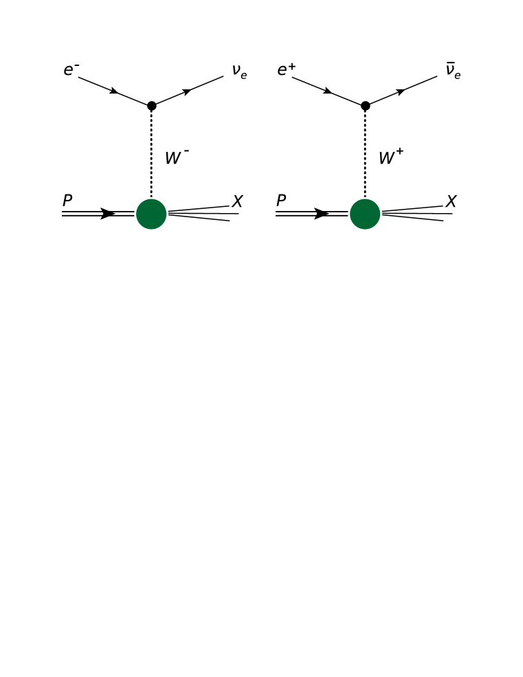
Figure 12: Schematic picture of charged-current neutrino production in DIS induced by an electron or positron on a proton.

The $F_{2}$ structure function for the CC reaction on a proton has the form

$$F_{2}^{W^{-}p}(x)=2x[u(x)+c(x)+{\overline{d}}(x)+{\overline{s}}(x)].$$ (52)

Of course, these reactions will occur at extremely high energies and very large $Q^{2}$, such that we assume corrections to the $F_{2}$ structure functions in Eq. (52) [and others] arising from quark mixing matrices, quark masses, or higher twist effects to be completely negligible.

We can also consider the corresponding reaction for positrons on protons, $(e^{+},{\overline{\nu}}_{e})$. This reaction involves the absorption of a $W^{+}$ on the proton, with the resulting $F_{2}$ structure function

$$F_{2}^{W^{+}p}(x)=2x[{\overline{u}}(x)+\bar{c}(x)+d(x)+s(x)].$$ (53)

Using Eqs. (52 & 53), we can straightforwardly calculate the $F_{2}$ structure functions (per nucleon) on the deuteron, finding

$$F_{2}^{W^{-}D}(x) = x[u^{+}(x)+d^{+}(x)+2c(x)+2{\overline{s}}(x)-\delta d(x)-\delta{\overline{u}}(x)]\ ;$$

$$F_{2}^{W^{+}D}(x) = x[u^{+}(x)+d^{+}(x)+2\bar{c}(x)+2s(x)-\delta{\overline{d}}(x)-\delta u(x)]\ .$$ (54)

Note that in Eq. (54) we have introduced combinations of quark parton distribution functions (PDFs) that are even or odd under charge conjugation, as well as the CSV PDFs

$$q^{\pm}(x) = q(x)\pm\bar{q}(x)\ ;$$

$$\delta u(x) = u^{p}(x)-d^{n}(x)\ ;$$

$$\delta d(x) = d^{p}(x)-u^{n}(x)\ .$$ (55)

There are analogous relations to Eq. (55) for the antiquark CSV PDFs, and for the remainder of this section we assume that ${\overline{c}}(x)=c(x)$ [actually, deviations away from this hypothesis will be presented systematically in Chap. 4]. The distributions $q^{-}(x)$, which involve the differences between quark and antiquark PDFs (alternatively, they are the $C$-odd combinations of quark distributions), are the valence parton distributions for a given quark flavor.

We now define the following quantity (the master-expression of this section),

$$R^{-}(x)\equiv\frac{2(F_{2}^{W^{-}D}(x)-F_{2}^{W^{+}D}(x))}{F_{2}^{W^{-}p}(x)+F_{2}^{W^{+}p}(x)}.$$ (56)

The quantity $R^{-}(x)$ is given by the difference in the $F_{2}$ structure functions per nucleon for electron-deuteron and positron-deuteron CC reactions, divided by the average $F_{2}$ structure function for CC reactions on protons initiated by electrons and by positrons.

Using Eqs. (52), (53) and (54) we can straightforwardly show that the quantity $R^{-}(x)$ in (56) has the form

$$R^{-}(x)=\frac{x[-2s^{-}(x)+\delta u^{-}(x)-\delta d^{-}(x)]}{x[u^{+}(x)+d^{+}(x)+s^{+}(x)+2c(x)]}\ .$$ (57)

Thus $R^{-}(x)$ is proportional to the valence quark CSV parton distributions plus the strange quark asymmetry (the difference between the strange and antistrange PDFs). Insofar as the strange quark asymmetry exists, it should be large only at quite small Bjorken $x<0.1$, while theoretical estimates of the valence CSV parton distributions [99, 100] suggest that for $Q^{2}\sim 10$ GeV² they peak at values $x\sim 0.4$.

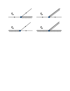
Figure 13: Schematic picture of quarks coupling to QCD gluons. This gives the origin of QCD splitting relevant for $C$-even parton distributions and gluons.

We thus consider a hypothetical collider with 50 GeV electrons or positrons colliding on protons and deuterons of roughly 7 TeV energy — similar to what might be achievable at a putative ‘LHeC-type’ machine. More specifically, we consider charged-current reactions at such a facility with $Q^{2}=10^{5}$ GeV², and simulate the two dominant mechanisms for charge symmetry violation in parton distribution functions. The first of these arises from radiation of a photon by a quark, such as is shown schematically in Fig. 14; such contributions were first calculated systematically by MRST [101] and Glück et al. [102]. QED corrections of this kind are analogous to the familiar couplings of gluons to quarks portrayed in Fig. 13, aside from the fact that photons do not exhibit self-coupling as do gluons. Inclusion of these ‘QED splitting’ terms will necessarily induce charge symmetry violation in parton distribution functions due to the differing electromagnetic (EM) couplings of the photon to up and down quarks.

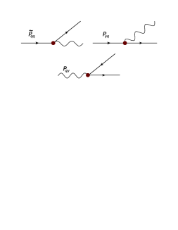
Figure 14: Schematic picture of quarks coupling to photons. This gives the origin of the QED splitting which produces CSV effects in parton distribution functions.

The behavior of parton distributions with increasing $Q^{2}$ is given by the DGLAP evolution equations [103, 104, 105]. We expand the DGLAP evolution equations to lowest order in both the strong coupling ${\alpha_{s}}$ and the electromagnetic coupling $\alpha$,

$$\frac{\partial q_{i}(x,\mu^{2})}{\partial\ln\mu^{2}} = {\frac{{\alpha_{s}}}{2\pi}}\left[P_{qq}\otimes q_{i}+P_{qg}\otimes g\right]+{\frac{\alpha}{2\pi}}e_{i}^{2}\widetilde{P}_{qq}\otimes q_{i}\ ;$$

$$\frac{\partial g(x,\mu^{2})}{\partial\ln\mu^{2}} = {\frac{{\alpha_{s}}}{2\pi}}\left[\sum_{j}P_{gq}\otimes q_{j}+P_{gg}\otimes g\right]+{\frac{\alpha}{2\pi}}e_{i}^{2}\widetilde{P}_{qq}\otimes q_{i}\ ;$$

$$\frac{\partial\gamma(x,\mu^{2})}{\partial\ln\mu^{2}} = {\frac{\alpha}{2\pi}}\sum_{j}e_{j}^{2}P_{\gamma q}\otimes q_{j}\ .$$ (58)

In Eq. (58), $q_{i}(x,\mu^{2})$ is the parton distribution for a given flavor $i$, $g(x,\mu^{2})$ is the gluon distribution, and $\gamma(x,\mu^{2})$ the photon parton distribution mentioned earlier [101]; these probability distributions are collectively bounded at some starting scale $Q^{2}=\mu^{2}$ by a global momentum conservation rule of the form

$$\int_{0}^{1}dx\ x\left\{\sum_{q}q(x,\mu^{2})\ +\ g(x,\mu^{2})\ +\ \gamma(x,\mu^{2})\right\}\ \equiv\ 1\ ,$$ (59)

where the convolutions in Eq. (58) we take to be

$$P\otimes q=\int_{x}^{1}\,\frac{dz}{z}P(z)\ q(\frac{x}{z},\mu^{2})\ .$$ (60)

The splitting functions themselves are given by

$$\widetilde{P}_{qq}(z) = \frac{P_{qq}(z)}{C_{F}}\ ;\hskip 8.5359ptP_{\gamma q}(z)\ =\ \frac{P_{gq}(z)}{C_{F}}\ ;$$

$$P_{q\gamma}(z) = \frac{P_{qg}(z)}{T_{R}}\ ;\hskip 8.5359ptP_{\gamma\gamma}(z)\ =\ \sum_{j}\frac{-2e_{j}^{2}}{3}\delta(1-z)\ .$$ (61)

Fortunately, the QCD probability distributions above are directly calculable from the amplitudes given in Fig. 13; at leading order we have

$$P_{qq}(z)=2\delta(1-z)-{4\over 3}(1+z)+{8\over 3}\left({1\over 1-z}-\delta(1-z)\cdot\int_{0}^{1}dz^{\prime}{1\over 1-z^{\prime}}\right)\ ,$$ (62a)

$$P_{gq}(z)={4\over 3}\left\{1+(1-z)^{2}\right\}\big{/}z\ ,$$ (62b)

$$P_{qg}(z)={1\over 2}\left\{z^{2}+(1-z)^{2}\right\}\big{/}z\ ,$$ (62c)

$$P_{gg}(z)=\left({11\over 2}-{N_{F}\over 3}\right)\delta(1-z) +6\ \bigg{\{}z(1-z)+{1\over z}-z$$

$$+\ \left({1\over 1-z}-\delta(1-z)\cdot\int_{0}^{1}dz^{\prime}{1\over 1-z^{\prime}}\right)\bigg{\}}\ ,$$ (62d)

while relations analogous to Eqs. (58 & 62) hold for antiquarks. Taking the valence combinations from Eq. (55), we obtain scaling relations for up and down valence quarks

$$\frac{\partial u^{-}(x,\mu^{2})}{\partial\ln\mu^{2}} = {\frac{{\alpha_{s}}}{2\pi}}P_{qq}\otimes u^{-}+\frac{2\alpha}{9\pi}\widetilde{P}_{qq}\otimes u^{-}\ ;$$

$$\frac{\partial d^{-}(x,\mu^{2})}{\partial\ln\mu^{2}} = {\frac{{\alpha_{s}}}{2\pi}}P_{qq}\otimes d^{-}+\frac{\alpha}{18\pi}\widetilde{P}_{qq}\otimes d^{-}$$ (63)

For the valence CSV parton distributions we desire on the other hand, since $\delta u^{-}(x)=u_{p}^{-}(x)-d_{n}^{-}(x)$, from Eq. (63) we may obtain the evolution equations to lowest order in ${\alpha_{s}}$ and $\alpha$,

$$\frac{\partial[\delta u^{-}(x,\mu^{2})]}{\partial\ln\mu^{2}} \approx {\frac{\alpha}{2\pi}}(e_{u}^{2}-e_{d}^{2})\widetilde{P}_{qq}\otimes u^{-}\ ;$$

$$\frac{\partial[\delta d^{-}(x,\mu^{2})]}{\partial\ln\mu^{2}} \approx -{\frac{\alpha}{2\pi}}(e_{u}^{2}-e_{d}^{2})\widetilde{P}_{qq}\otimes d^{-}\ .$$ (64)

Eqs. (63 & 64) describe how the valence and CSV quark distributions respectively evolve with $Q^{2}$, to lowest order in both ${\alpha_{s}}$ and $\alpha$. Note that the total strength of the CSV effect as embodied by the first moments $\int_{0}^{1}dx\ \delta q^{-}$ is preserved (approximately) under $Q^{2}$ evolution by Eq. (55). Physically, the above formalism establishes that, with increasing $Q^{2}$, partons radiate gluons and photons which carry off momentum; since the total momentum fraction carried by quarks is given by the second moment of the parton distributions, as $Q^{2}$ increases, the parton distribution functions will shift towards progressively smaller $x$.

Comparison of Eqs. (63) and (64) makes clear that the radiation from valence quarks will be greater than that from the valence CSV distributions. This occurs because to lowest order in ${\alpha_{s}}$ and $\alpha$, valence quark evolution contains contributions from both gluon and photon radiation, whereas the valence CSV distribution has only a single term from photon radiation. This suggests that with increasing $Q^{2}$, the valence parton distributions would experience a larger shift to low $x$ than would the valence CSV distributions. We note that the quantity $R^{-}(x)$ defined in Eq. (57) is proportional to the ratio of valence CSV distributions to valence PDFs, at a given $x$ value. Thus, if the CSV valence distributions are becoming large relative to the valence PDFs at high $Q^{2}$, we expect the quantity $R^{-}(x)$ to grow as $Q^{2}$ increases; specifically one would expect the ratio to increase logarithmically with $Q^{2}$.

Eq. (64), the QCD evolution equations for the valence CSV parton distributions, have been solved by Glück et al. [102] and also by MRST [101]; both made slightly different approximations for the initial conditions, and we point out that while the effect of photon radiation is clear, it is far less obvious that the boundary conditions imposed on the calculations are appropriate. That is to say, it is not unambiguous a priori that low scales typical of quark models necessarily represent the appropriate place to set the CSV effect to zero. Therefore, in the absence of a compelling theoretical derivation it would extremely helpful to test the idea experimentally.

As stated, MRST [101] confronted this method with experimental data by explicitly including QED effects in the DGLAP equations via the photon distribution $\gamma(x,Q^{2})$ introduced in Sec. 3 with a scale dependence determined by Eq. (58). Specifically, MRST aimed to identify this quantity in the direct photon production process $ep\rightarrow e\gamma X$ where the final state $e$ and $\gamma$ are produced with equal and opposite large transverse momentum. This mechanism has been observed by the ZEUS Collaboration in $ep$ collisions at $\sqrt{s}=300$ and 318 GeV [106]. The observed cross sections were in reasonable agreement with the MRST calculations but disagreed with calculations done using the Monte Carlo simulations PYTHIA [107] and HERWIG [108]. Again, it would hence be useful to have other experimental tests of this method for including radiation of photons by partons, and the experiment suggested here could provide additional confirmation of this method.

The second source of valence parton CSV we consider arises naturally from the mass difference between the $u$ and $d$ quarks and may be calculated within light cone quark models. Formally, models [69, 109, 110] generally specify the quark distributions in a fashion similar to the derivation of $\Phi_{q,\bar{q}}$ in Chap. 1.1:

$$q(x,\mu^{2})\ =\ {1\over 4\pi}\ \int d\xi e^{-iMx\xi}\ \langle N|\gamma^{+}\psi^{\dagger}(\xi^{-})\gamma^{+}\psi(0)|N\rangle\ \hskip 28.45274pt\implies$$ (65a)

$$=\ {1\over 2}\sum_{X}\,\int{d^{3}k\over 2E_{k}(2\pi)^{3}}\ |\langle X|\frac{1+\gamma^{0}\gamma^{3}}{2}\psi(0)|N\rangle|^{2}\,\times\,\delta(M(1-x)-p_{X}^{+})\ ,\ \ \mathrm{and}$$ (65b)

$$\bar{q}(x,\mu^{2})\ =\ {1\over 2}\sum_{X}\,\int{d^{3}k\over 2E_{k}(2\pi)^{3}}\ |\langle X|\frac{1+\gamma^{0}\gamma^{3}}{2}\psi^{\dagger}(0)|N\rangle|^{2}\,\times\,\delta(M(1-x)-p_{X}^{+})\ ,$$ (65c)

by which we conclude the light-front result for the $q_{v}(x)=q(x)-\bar{q}(x)$ valence-type distributions to be

$$q_{v}(x,\mu^{2})\ =M\sum_{X}\,|\langle X|\frac{1+\gamma^{0}\gamma^{3}}{2}\psi_{v}(0)|N\rangle|^{2}\,\times\,\delta(M(1-x)-p_{X}^{+})\ ,$$ (66)

where we have defined the field of the valence quark as $\psi_{v}\mathrel{\vbox{\hbox{\scriptsize.}\hbox{\scriptsize.}}}=\psi-\psi^{\dagger}$, and an explicit linear dependence on the nucleon mass $M$ has issued due to the fact that $dk^{+}=Mdx$ in the integration measures of Eq. (65).

Technically, Eq. (66) denotes the process where a valence quark is removed from a nucleon $|N\rangle$, and the result is summed over all final states $|X\rangle$. The quantity $p_{X}^{+}$ is the energy of the state following removal of a valence quark with momentum $k$, while $\mu^{2}$ represents the starting value for the $Q^{2}$ evolution of the parton distributions. Eq. (66) is formally exact and provides a natural starting point for calculations which provide the correct support to the PDFs.

Model quark wavefunctions are found to be nearly invariant under the small mass changes typical of CSV [100], so we concentrate on the breaking of partonic charge symmetry associated with energy shifts resulting from $u$ and $d$ quark mass differences. In particular, we consider the effect of the $n-p$ mass difference $\delta M\equiv M_{n}-M_{p}=1.3$ MeV, as well as the difference in diquark masses arising from the current quark mass difference between up and down quarks. We define the quantity

$${\delta\widetilde{m}}=m_{dd}-m_{uu}\,,$$ (67)

for which we have a robust estimate ${\delta\widetilde{m}}\sim 4$ MeV [111]. We determine CSV valence PDFs by calculating the variation of quark model parton distributions in Eq. (66) with respect to these quantities, i.e.,

$$\delta q_{v}\approx\frac{\partial q_{v}}{\partial({\delta\widetilde{m}})}{\delta\widetilde{m}}+\frac{\partial q_{v}}{\partial(\delta M)}\delta M\ .$$ (68)

Using the last relation, the valence charge symmetry violating parton distributions may be obtained by evaluating variations with respect to diquark and nucleon masses of quark model valence parton distributions. The resulting PDFs then account for the quark and nucleon mass differences that generate CSV effects.

In practice, we compute using the approach first developed by Sather [99], which is founded upon a static quark picture that ignores partonic transverse momentum $k_{\perp}$. On the down side, such models do not necessarily ensure the desire support in the quark distributions, but for our purposes the Sather prescription gives numerically similar results when compared with alternative models [100] that do not possess this limitation. By applying Eq. (68) to Eq. (66) within this scheme, an analytic approximation relating valence quark CSV to derivatives of the valence PDFs emerges. For instance, the Sather prescription approximates the CSV effect in the $u_{v}(x)$ distribution due to the nucleon mass difference $\delta M$ as

$$\delta u^{M}(x,Q^{2}_{0})\ \approx\ -{|\delta M|\over M}\ \left(u_{v}(x,Q^{2}_{0})+\{x-1\}\cdot{du_{v}(x,Q^{2}_{0})\over dx}\right)\ .$$ (69)

As a rule, the analytic approximation of Sather is appropriate only at $Q^{2}$ values appropriate for quark model calculations, i.e., $Q^{2}\sim 0.25-0.5$ GeV².

We hence proceed with the Sather prescription, differentiating valence parton distribution functions to obtain valence CSV PDFs. For this purpose we use the MRST2001 parton distributions [112] at the starting scale, $Q_{0}^{2}=1$ GeV². This is slightly too large a value of $Q^{2}$ for the validity of Sather’s analytic approximation, but the resulting errors should be small. We then insert the resulting CSV PDFs into the DGLAP evolution equations and evolve to the $Q^{2}$ appropriate for the electron collider experiments, finding results similar to those obtained using the CSV distributions of Rodionov et al..

Since the CSV effects arising from QED splitting effects and from quark mass differences are essentially independent, we simply add the two effects directly to produce an overall CSV effect.

Finally, there is one additional term that enters into the quantity $R^{-}(x)$ of Eq. (57), namely, the strange quark momentum asymmetry [113, 114]

$$xs^{-}(x)\equiv x[s(x)-\overline{s}(x)]\ .$$ (70)

Strange (antistrange) parton distributions can be measured through opposite-sign dimuon production initiated by neutrinos (antineutrinos). A neutrino undergoes a charged-current reaction, producing a $\mu^{-}$ and a $W^{+}$, which is then absorbed on an $s$ quark producing a charm quark. The charm quark subsequently undergoes a semileptonic decay producing a $\mu^{+}$ and an $s$ quark. The cross section for this process is proportional to the strange quark distribution. The corresponding reaction initiated by an antineutrino measures the antistrange PDF.

Dimuon cross sections have been measured by the CCFR [115] and NuTeV [116] experiments, by which one might extract the quantity $xs^{-}(x)$. These analyses have been undertaken by five groups: CTEQ [117]; Mason et al. [118]; the NNPDF Collaboration [119]; MSTW [120]; and Alekhin, Kulagin and Petti [121]. Hence, to control the potential contributions to $R^{-}$ from strangeness asymmetries, we exploited the NuTeV neutrino analysis of Mason et al. by constructing an analytic fit to the results of Ref. [118] at $Q^{2}=16$ GeV² with the form

$$xs^{-}(x)=Ax^{b}\exp{(-cx)}\cdot(x-0.004)\ .$$ (71)

The resulting strange quark asymmetry was then inserted into the DGLAP evolution equation and evolved to the putative LHeC scale.

Figure 15: (Left) Parton distributions that occur in the numerator of Eq. (57). Solid curve: $x\delta u^{-}(x)$; long-dashed curve: $x\delta d^{-}(x)$; short-dashed curve: $xs^{-}(x)$. The PDFs have been evolved to $Q^{2}=10^{5}$ GeV². (Right) Contributions to the quantity $R^{-}(x)$ vs. $x$ from Eq. (57), where the PDFs are evolved to $Q^{2}=10^{5}$ GeV². Solid curve: contribution from QED splitting parton CSV term only; long-dashed curve: includes contribution also from quark mass CSV term; short-dashed curve: contribution from all terms including strange quark asymmetry.

Having gathered the requisite pieces, the parton distribution functions that occur in the numerator of Eq. (57) are plotted in the left panel of Fig. 15. The solid black curve is $x\delta u^{-}(x)$, the red long-dashed curve is $x\delta d^{-}(x)$, and the blue short-dashed curve is $xs^{-}(x)$. As one might expect, the valence CSV distributions peak at a relatively large value $x\sim 0.2$, while the strange quark asymmetry peaks at an extremely small $x$ value. Note that due to valence quark normalization [as defined in Eq. (4)], all of these quantities must have zero first moment, i.e., $\langle q(x)\rangle=0$, where $q=[\delta u^{-},\delta d^{-},s^{-}]$. The strange quark asymmetry has zero first moment because the proton has no net strangeness; the valence CSV distributions must have zero first moment because otherwise this would change the total number of valence quarks in the neutron. As a result, each of these curves must cross zero at a small value of $x$ (not shown in Fig. 15).

Another notable point is that the signs of these quantities are such that (for values of $x$ above the crossover point for all of the parton distributions) all three contributions should add together in the numerator of Eq. (57). The right panel of Fig. 15 shows the expected value of $R^{-}(x)$ vs. Bjorken $x$. The solid curve on the right of Fig. 15 includes only the QED splitting contribution to partonic CSV. The long-dashed curve includes both QED splitting and quark mass contributions to valence quark CSV, while the short-dashed curve includes all three terms in the numerator of Eq. (57), including also the contribution from strange quark asymmetry.

Figure 16: A comparison of the CSV effects generated only by the MRSTQED breaking evolved via Eq. (63) to the putative LHeC scale with the more restrained kinematics of a first- and second-stage medium energy electron-ion colliders described in-text.

We see that for large $x>0.2$ the strange quark contribution is essentially negligible,but the predicted values of $R^{-}(x)$ are considerable: for $x=0.6$ the calculated ratio is greater than 6%. This is quite a sizable result for partonic CSV terms, which for most observables yield effects at the 1% level or smaller [95]. This confirms our argument that, while both the valence quark and valence CSV distributions shift to lower $x$ values with increasing $Q^{2}$, the CSV distributions experience a smaller shift (because to lowest order the CSV valence distributions only radiate photons while the valence parton PDFs radiate both gluons and photons), and thus for a given $x$ the ratio of valence CSV distributions to valence PDFs should increase slowly with $Q^{2}$. Our best theoretical estimate of the ratio $R^{-}(x)$ from Eq. (57) at large $x$ values is predicted to be rather large, of the order of several percent. For reasonably large values $x>0.1$, the ratio $R^{-}(x)$ is composed of relatively equal contributions from valence parton CSV effects arising from quark mass differences and from QED radiation. Thus the quantitative values obtained for the ratio $R^{-}(x)$ can provide a further check on the assumptions made in determining charge symmetry violation arising from QED radiation.

We finish up with one additional observation: significant partonic CSV signals embodied by $R^{-}(x,Q^{2})$ may in fact not even require the vaunted kinematics of a hypothetical LHeC-type machine. This is suggested by the $x$ dependence plotted in Fig. 16, wherein we compare the QED-generated contributions to $R^{-}$ at LHeC with the same computation at the more restricted kinematics of lower-energy machines [98], labeled ‘EIC-1’ and ‘EIC-2.’ For each, we assume the collision of $5,\,20$ GeV electrons on $20,\,250$ GeV deuterons at $Q^{2}=300,\,2000$ GeV² and center-of-mass energy $\sqrt{s}=45,\,140$ GeV, respectively. The fact that the lower energy curves quite closely tract the LHeC prediction signifies that the evolution enhancements to $R^{-}$ may not require such large intervals in $Q^{2}$ to become apparent, bolstering the accessibility of these effects at more modest kinematics; at the same time, the event rates corresponding to the $W$ exchange mechanisms of Eq. (54) remain to be estimated, and must be carefully simulated in the future.

It would therefore seem that a hypothetical high energy electron/positron collider whose beams interact with deuteron beams from the LHC may produce the most promising observable with which to search for partonic charge symmetry violating effects, although less energetic reactions may also be useful.

Chapter 3 Mass corrections to DIS

“Principles
You can’t say A is made of B
or vice versa.
All mass is interaction.”
      — Richard P. Feynman

Independent of the inherent interest in extending and strengthening the preceding formalism to analyze hadronic interactions, traditional DIS continues to build upon its earlier successes by probing new regions of experimental phase space. While the perturbative domain of large $Q^{2}$ and small parton momentum fraction $x$ has received considerable attention both experimentally and theoretically, the previous chapter demonstrated that the region of large $x$ and low $Q^{2}$ ($\sim 1-2$ GeV²), involves various nonperturbative effects which remain comparatively unexplored. This is perhaps unsurprising given the difficulty in reliably computing the various corrections that are needed to describe data in this region. Among the more vexing of these nonperturbative dynamics are the effects due to target mass corrections (TMCs) associated with finite values of $M^{2}/Q^{2}$, where $M$ is the nucleon mass, as well as higher twist terms arising from long-range nonperturbative multi-parton correlations.

This is particularly relevant for imminent proposed measurements at Jefferson Lab [124, 125, 126] and elsewhere, which seek to probe very large $x$ ($x\sim 0.85$) and provide improved access to many of the observables described in Chap. 2: the ratio of $d$ to $u$ quark distributions, partonic CSV, and SM tests in parity-violating asymmetries. Aside from this, better knowledge of PDFs at large $x$ is imperative in searches for new physics signals at collider experiments such as those of the Tevatron or LHC at large rapidities or for heavy mass particles [127], as well as at more central rapidities where uncertainties in large-$x$ PDFs at low $Q^{2}$ can, through $Q^{2}$ evolution, affect cross sections at small $x$ and large $Q^{2}$ [128].

1 Kinematical Higher Twist Effects

Among these effects, the most amenable to direct computation are, in principle, the TMCs, as well as their more general counterpart in semi-inclusive reactions, hadron mass corrections (HMCs). Therefore, drawing upon the findings of [129], we present in this chapter a systematic analysis of several frameworks for the computation of TMCs/HMCs, and assess the phenomenological impact on DIS observables of especial importance.

In Sec. 2 we summarize the main results for TMCs in the OPE and collinear factorization (CF) formulations for the $F_{1}$, $F_{2}$, $F_{3}$ and $F_{L}$ structure functions at NLO, and exhibit some numerical examples. Implications for various observables are discussed in Sec. 3, with special attention given to the longitudinal to transverse cross section ratios $R$, and parity-violating (PV) DIS asymmetries on the proton and deuteron, which are sensitive to $\gamma Z$ interference structure functions. We also quantify the effects of perturbative NLO corrections on the $R^{\gamma Z}$ ratio for the $\gamma Z$ interference, about which essentially nothing is known empirically. We conclude the chapter by extending our mass correction prescriptions to the more general setting of semi-inclusive DIS (SIDIS). As a slightly more exclusive counterpart to fully inclusive DIS, SIDIS by definition implies the production of specific final state hadrons, which necessitates a more subtle formalism for simultaneously incorporating both the initial and final state hadron masses. In Sec. 4 we present the contours of just such a model, developed in [142], which exploits the properties of CF as formulated in momentum space.

2 Target Mass Corrections

In this section we review the kinematic corrections to structure functions arising from scattering at finite values of $Q^{2}/\nu^{2}$. We consider several frameworks for the TMCs, including the conventional one based on the operator product expansion of Chap. 1.3, and various approximations to it, as well as a number of prescriptions using collinear factorization at leading and next-to-leading order in $\alpha_{s}$.

As discussed by Nachtmann [130], these target mass effects, sometimes called “kinematical higher twists” are in fact associated with leading twist operators (hence contain no additional information on the nonperturbative parton correlations), even though they give rise to $Q^{2}/\nu^{2}=4x^{2}M^{2}/Q^{2}$ corrections, where $\nu=Q^{2}/2Mx$ is the energy transfer. Nachtmann further showed that one could generalize the standard operator product expansion (OPE) of structure function moments to finite $Q^{2}$ such that only operators of a specific twist would appear at a given order in $1/Q^{2}$. The resulting target mass corrected structure functions can then be derived through an inverse Mellin transformation, as shown by Georgi and Politzer [131] and demonstrated below (for a thorough review of TMCs in the OPE approach see Ref. [44]).

Later, an alternative formulation in terms of collinear factorization (CF) was used by Ellis, Furmanski and Petronzio [132] to derive TMCs including the effects of off-shell partons and parton transverse motion. While the OPE and CF formulations yield identical results for leading twist PDFs, they differ in the details of how the target mass corrections are manifested at finite $Q^{2}$. Other versions of TMCs were subsequently derived [133, 134, 135] within the CF formalism using various assumptions about the intrinsic properties of partons and higher twist contributions, leading to rather large differences in some cases [135].

In any case, the structure functions for the scattering of an unpolarized lepton from an unpolarized nucleon are defined in terms of the nucleon hadron tensor introduced in Eq. (9),

$$W_{\mu\nu} = {1\over 4\pi}\int d^{4}z\,e^{iq\cdot z}\langle P\left|\left[J_{\mu}^{\dagger}(z),J_{\nu}(0)\right]\right|P\rangle$$ (1b)

$$= \left(-g_{\mu\nu}+\frac{q_{\mu}q_{\nu}}{q^{2}}\right)F_{1}(x,Q^{2})\ +\ \left(p_{\mu}-\frac{p\cdot q}{q^{2}}q_{\mu}\right)\left(p_{\nu}-\frac{p\cdot q}{q^{2}}q_{\nu}\right){F_{2}(x,Q^{2})\over p\cdot q}$$

$$-\ i\epsilon_{\mu\nu\alpha\beta}q^{\alpha}p^{\beta}\frac{F_{3}(x,Q^{2})}{2p\cdot q}\,,$$

where again $J_{\mu}$ is the electromagnetic or weak current operator for a given virtual boson ($\gamma$, $Z$ or $W^{\pm}$). Here $P$ and $q$ are again the nucleon and exchanged boson $4$-momenta, respectively, with $q^{2}=-Q^{2}$ as before.

The structure functions $F_{1,2}$ are related to the product of two vector or two axial-vector currents, while $F_{3}$ arises from the interference of vector and axial-vector currents. The $F_{1}$ structure function is proportional to the transverse virtual boson cross section, and $F_{2}$ is given by a combination of transverse and longitudinal cross sections. It is convenient to also study the longitudinal structure function introduced in Chap. 2,

$$F_{L}(x,Q^{2})\ =\ \rho^{2}F_{2}(x,Q^{2})-2xF_{1}(x,Q^{2})\,,$$ (2)

where

$$\rho^{2}\ =\ 1+\frac{4x^{2}M^{2}}{Q^{2}}\ \equiv\ r^{2}\ ,$$ (3)

with $r^{2}=1+Q^{2}/\nu^{2}$ having been used in Chap. 2. In the following we will summarize target mass corrections for each of these structure functions computed within the various approaches outlined above.

1 Operator product expansion

Target mass corrections to structure functions were first systematically considered by Georgi and Politzer [131] in the framework of the operator product expansion, and in the current section we reprise the essential details of their formalism. Actually, the basic foundation has already been introduced in Chap. The nonperturbative structure of hadrons.3 in which we outlined the main idea involving the expansion of the current operators of Eq. (1) into the general form presented in Eq. (45).

Formally, the OPE generates mass-dependent $1/Q^{2}$ corrections by introducing covariant derivatives into the twist-two quark bilinears of $J_{\mu}J_{\nu}$ in Eq. (1b): $\bar{\psi}\gamma^{\mu}D^{\mu_{1}}\cdots D^{\mu_{N}}\psi$; since each derivative $D^{\mu_{i}}$ increases both the dimension and spin of the operator by one unit, the twist (dimension minus spin) remains unchanged. Rather than the simple expression of Eq. (46),this practice demands a more complicated expansion of $\langle N(P)|\ \mathcal{O}^{\mu_{1}\dots\mu_{N}}_{i}(0)\ |N(P)\rangle$ — one that explicitly incorporates the $g^{\mu_{a}\mu_{b}}$ trace terms responsible for $1/Q^{2}$ corrections.

Making the replacement $N\rightarrow 2k$ in the language of [131], we can rearrange Eq. (46) as

$$\Pi^{\mu_{1}\ \dots\ \mu_{2k}} \mathrel{\vbox{\hbox{\scriptsize.}\hbox{\scriptsize.}}}=\langle N(P)|\ \mathcal{O}^{\mu_{1}\dots\mu_{2k}}_{i}(0)\ |N(P)\rangle$$

$$=\ \sum_{j=0}^{k}\ (-1)^{j}\ {(2k-j)!\over 2^{j}\ (2k)!}\ g\ \dots\ g\,\,P\ \dots\ P\ ,$$ (4)

where $g\ \dots\ g$ refers to a symmetric combination of $j$ metric terms $\sim g^{\mu_{a}\mu_{b}}$, while the $P\ \dots\ P$ is a product of $2k-2j$ factors of $P^{\mu_{a}}$. Note that the ‘trace terms’ mentioned in, e.g., Eq. (46) are thus accounted for by the $j>0$ contributions inside the summation of Eq. (4). By the same logic on the other hand, taking only the $j=0$ term recovers the leading contribution to the OPE found in Chap. 1.3 —

$$\Pi^{\mu_{1}\ \dots\ \mu_{2k}}=P^{\mu_{1}}\ \dots\ P^{\mu_{2k}}\ .$$ (5)

The calculation is then carried forward by inserting the expansion of Eq. (4) into the RHS for the OPE of $T_{\mu\nu}$ given in Eq. (45). The contributions for specific structure functions moments may be isolated from Eq. (4) by projecting the coefficients of the tensor structures $\kappa^{L,2,3}_{\mu\nu}$ defined in Eq. (48); for instance, projecting the coefficient of $\kappa^{2}_{\mu\nu}$ and keeping track of combinatoric factors as shown in [131] results in

$$\int_{0}^{1}dx\ x^{N-2}\ F^{\rm OPE}_{2}(x,Q^{2})\ =\ \sum_{j=0}^{\infty}\left({P^{2}\over Q^{2}}\right)^{j}{(N+j)!\over j!(N-2)!}\ {A^{(N+2j)}\cdot C^{N+2j}_{2}\over(N+2j)!\ (N+2j-1)!}\ ,$$

$$=\ \sum_{j=0}^{\infty}\left({M^{2}\over Q^{2}}\right)^{j}{(N+j)!\over j!(N-2)!}\ {M^{(0),\ N+2j}_{2}\over(N+2j)!\ (N+2j-1)!}\ ,$$ (6)

in which on-shellness of the nucleon grants $P^{2}=M^{2}$. In Eq. (6), we have recognized the fact that the matrix elements $A^{(N+2j)}$ are due to the correlated quark fields inside the nucleon; for our purposes here, we can relate them back to the “massless” structure functions of Eq. (54):

$$A^{(N+2j)}\cdot C^{N+2j}_{2}\ =\ M^{(0),\ N+2j}_{2}\ =\ \int_{0}^{1}dz\ z^{N+2j-2}\ F^{(0)}_{2}(z)\ ,$$ (7)

whence the second line of Eq. (6) follows.

It remains only to unfold the resulting target mass corrected structure functions. This may be accomplished by means of an inverse Mellin transformation; i.e., generically, for a suitably analytic function $f(x)$,

$$M^{n}\ =\ \int_{0}^{1}dx\ x^{n-1}\ f(x)\ \implies\ f(x)\ =\ {1\over 2\pi i}\int_{-i\infty}^{+i\infty}dn\ x^{-n}\ M^{n}\ .$$ (8)

Applying this transform to extract $F^{\rm OPE}_{2}(x,Q^{2})$ from Eq. (6) at last yields the desired result:

$$F_{2}^{\rm OPE}(x,Q^{2})={(1+\rho)^{2}\over 4\rho^{3}}F_{2}^{(0)}(\xi,Q^{2})\ +\ {3x(\rho^{2}-1)\over 2\rho^{4}}\left[h_{2}(\xi,Q^{2})+{\rho^{2}-1\over 2x\rho}g_{2}(\xi,Q^{2})\right]\ .$$ (9)

A very similar procedure suffices for the other $F^{\rm OPE}_{i}(x,Q^{2})$ [131], which we tabulate for completeness:

$$F_{1}^{\rm OPE}(x,Q^{2}) = {1+\rho\over 2\rho}F_{1}^{(0)}(\xi,Q^{2})\ +\ {\rho^{2}-1\over 4\rho^{2}}\left[h_{2}(\xi,Q^{2})+{\rho^{2}-1\over 2x\rho}g_{2}(\xi,Q^{2})\right],$$

$$F_{L}^{\rm OPE}(x,Q^{2}) = {(1+\rho)^{2}\over 4\rho}F_{L}^{(0)}(\xi,Q^{2})+\ {x(\rho^{2}-1)\over\rho^{2}}\left[h_{2}(\xi,Q^{2})+{\rho^{2}-1\over 2x\rho}g_{2}(\xi,Q^{2})\right],$$

$$F_{3}^{\rm OPE}(x,Q^{2}) = {(1+\rho)\over 2\rho^{2}}F_{3}^{(0)}(\xi,Q^{2})+\ {(\rho^{2}-1)\over 2\rho^{3}}h_{3}(\xi,Q^{2}).$$ (10)

Again, $F_{i}^{(0)}$ are the structure functions in the “massless” $M^{2}/Q^{2}\to 0$ limit, evaluated at the modified scaling variable $\xi$ [130, 138],

$$\xi={2x\over 1+\rho}\,,$$ (11)

which approaches $x$ as $M^{2}/Q^{2}\to 0$. The functions $h_{2}$, $g_{2}$ and $h_{3}$ are associated with higher order terms in $M^{2}/Q^{2}$ and are given by [131, 44]

$$h_{2}(\xi,Q^{2}) = \int_{\xi}^{1}du\,{F_{2}^{(0)}(u,Q^{2})\over u^{2}}\,,$$ (12a)

$$g_{2}(\xi,Q^{2}) = \int_{\xi}^{1}du\,\int_{u}^{1}dv{F_{2}^{(0)}(v,Q^{2})\over v^{2}}\ =\ \int_{\xi}^{1}du\,(u-\xi){F_{2}^{(0)}(u,Q^{2})\over u^{2}}\,,$$ (12b)

$$h_{3}(\xi,Q^{2}) = \int_{\xi}^{1}du\,{F_{3}^{(0)}(u,Q^{2})\over u}\,.$$ (12c)

(Note that the function $g_{2}$ here should not be confused with the spin-dependent $g_{2}$ structure function measured in polarized lepton–nucleon scattering.)

The expressions in Eqs. (10) are known to suffer from the “threshold problem”, in which the target mass corrected (leading twist) structure functions do not vanish as $x\to 1$, and are in fact nonzero in the kinematically forbidden $x>1$ region, where for a proton target baryon number conservation would be violated. This is clear from the ${\cal O}(1)$ terms in Eqs. (10) in which the massless functions $F_{i}^{(0)}$ are evaluated at $\xi$. Because at any finite $Q^{2}$ value one has $\xi<\xi_{0}\equiv\xi(x=1)<1$, for any input function $F_{i}^{(0)}$ which is nonzero for $0<x<1$, the target mass corrected function at $x=1$ will not vanish, $F_{i}^{\rm OPE}(x=1,Q^{2}<\infty)>0$. A number of attempts have been made to ameliorate the threshold problem [139, 140] using various prescriptions and ansätze, although none of these is unique and without additional complications [44].

Recently, Kulagin and Petti [141] showed that by expanding the target mass corrected structure functions to leading order in $1/Q^{2}$, the resulting functions have the correct $x\to 1$ limits,

$$F_{1}^{1/Q^{2}}(x,Q^{2}) = \frac{1}{4}\left(5-\rho^{2}\right)F_{1}^{(0)}(x,Q^{2})\ -\ \frac{1}{4}\left(\rho^{2}-1\right)\left[xF_{1}^{(0)\,\prime}(x,Q^{2})-\ h_{2}(x,Q^{2})\right],$$

$$F_{2}^{1/Q^{2}}(x,Q^{2}) = \left(2-\rho^{2}\right)F_{2}^{(0)}(x,Q^{2})\ -\ \frac{1}{4}\left(\rho^{2}-1\right)\left[xF_{2}^{(0)\,\prime}(x,Q^{2})-\ 6xh_{2}(x,Q^{2})\right],$$

$$F_{L}^{1/Q^{2}}(x,Q^{2}) = F_{L}^{(0)}(x,Q^{2})\ -\ \frac{1}{4}\left(\rho^{2}-1\right)\left[xF_{L}^{(0)\,\prime}(x,Q^{2})-\ 4xh_{2}(x,Q^{2})\right],$$

$$F_{3}^{1/Q^{2}}(x,Q^{2}) = \frac{1}{4}\left(7-3\rho^{2}\right)F_{3}^{(0)}(x,Q^{2})\ -\ \frac{1}{4}\left(\rho^{2}-1\right)\left[xF_{3}^{(0)\,\prime}(x,Q^{2})-\ 2h_{3}(x,Q^{2})\right].$$

While avoiding the threshold problem, this prescription, however, raises the question of whether the $1/Q^{2}$ approximation is sufficiently accurate for structure functions near $x\approx 1$ at moderate $Q^{2}$. To test the convergence of the $1/Q^{2}$ expansion at large $x$, we further expand the OPE results (10) to include ${\cal O}(1/Q^{4})$ corrections,

$$F_{1}^{1/Q^{4}}(x,Q^{2}) = F_{1}^{1/Q^{2}}(x,Q^{2})\ +\ \left(\rho^{2}-1\right)^{2}\left[\frac{3}{16}F_{1}^{(0)}(x,Q^{2})\ +\ \frac{1}{16x}F_{2}^{(0)}(x,Q^{2})\right.$$

$$+ \left.\frac{3x}{16}F_{1}^{(0)\,\prime}(x,Q^{2})\ +\ \frac{x^{2}}{32}\,F_{1}^{(0)\,\prime\prime}(x,Q^{2})\ -\ \frac{1}{4}\,h_{2}(x,Q^{2})\ +\ \frac{1}{8x}\,g_{2}(x,Q^{2})\right]$$

$$F_{2}^{1/Q^{4}}(x,Q^{2}) = F_{2}^{1/Q^{2}}(x,Q^{2})\ +\ \left(\rho^{2}-1\right)^{2}\left[\frac{23}{16}F_{2}^{(0)}(x,Q^{2})\ +\ \frac{3x}{8}F_{2}^{(0)\,\prime}(x,Q^{2})\right.$$

$$+ \left.\frac{x^{2}}{32}\,F_{2}^{(0)\,\prime\prime}(x,Q^{2})\ -\ 3x\,h_{2}(x,Q^{2})\ +\ \frac{3}{4}\,g_{2}(x,Q^{2})\right],$$

$$F_{L}^{1/Q^{4}}(x,Q^{2}) = F_{L}^{1/Q^{2}}(x,Q^{2})\ +\ \left(\rho^{2}-1\right)^{2}\left[\frac{3}{16}F_{L}^{(0)}(x,Q^{2})\ +\ \frac{1}{4}F_{2}^{(0)}(x,Q^{2})\right.$$

$$+ \left.\frac{x}{8}F_{L}^{(0)\,\prime}(x,Q^{2})\ +\ \frac{x^{2}}{32}F_{L}^{(0)\,\prime\prime}(x,Q^{2})\ -\ xh_{2}(x,Q^{2})\ +\ \frac{1}{2}g_{2}(x,Q^{2})\right],$$

$$F_{3}^{1/Q^{4}}(x,Q^{2}) = F_{3}^{1/Q^{2}}(x,Q^{2})\ +\ \left(\rho^{2}-1\right)^{2}\left[\frac{13}{16}F_{3}^{(0)}(x,Q^{2})+\ \frac{5x}{16}F_{3}^{(0)\,\prime}(x,Q^{2})\right.$$ (14)

$$+ \left.\frac{x^{2}}{32}\,F_{3}^{(0)\,\prime\prime}(x,Q^{2})\ -\ \frac{3}{4}\,h_{3}(x,Q^{2})\right],$$

where the first $(F_{i}^{(0)\,\prime})$ and second $(F_{2}^{(0)\,\prime\prime})$ derivatives of the structure functions are with respect to $x$. In fact, one can show that for a structure function that behaves at large $x$ as $(1-x)^{n}$, the target mass corrected result will vanish in the $x\to 1$ limit up to order $1/Q^{2n-2}$ in the expansion. For $n\approx 3$, as is typical for nucleon structure functions, the threshold problem will therefore appear only at order $1/Q^{6}$.

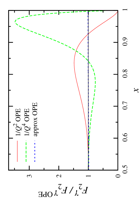
Figure 1: Ratio of the target mass corrected $F_{2}$ structure functions using the $1/Q^{2}$ (solid, red), $1/Q^{4}$ (long-dashed, green) and phenomenological (short-dashed, blue) OPE approximations compared with the exact OPE result, Eq. (9), at $Q^{2}=2$ GeV². Note that the phenomenological OPE approximation is almost indistinguishable from the exact OPE result, while the $1/Q^{2}$ and $1/Q^{4}$ expansions deviate from this for $x\gtrsim 0.6$.

The accuracy of the $1/Q^{2}$ expansions is illustrated in Fig. 1, where in order to isolate the target mass effect from the specific form of the structure function parametrization we have taken for simplicity the form $F_{2}\sim(1-x)^{3}$ and computed at a fixed $Q^{2}=2$ GeV². Both the $1/Q^{2}$ and $1/Q^{4}$ approximations are found to reproduce the full OPE result very well up to $x\approx 0.6$, but significant deviations are visible at larger $x$. Furthermore, while there is a modest improvement in the agreement with the exact result for $0.6\lesssim x\lesssim 0.8$ after inclusion of the $1/Q^{4}$ terms, both expansions appear to break down for $x\gtrsim 0.8$. The reliability of a low order $1/Q^{2}$ expansion is therefore questionable at these $x$ values, and hence their efficacy in removing the $x\to 1$ threshold problem.

Since the integrals in the functions $h_{2,3}$ and $g_{2}$ can be time consuming to compute numerically, Schienbein et al. [44] isolated phenomenological analytic forms which approximate the target mass corrected $F_{2}$ and $F_{3}$ structure functions in Eqs. (9) and (10) by

$$F_{2}^{\rm approx}(x,Q^{2}) = \frac{(1+\rho)^{2}}{2\rho^{3}}\left(1+\frac{3(\rho^{2}-1)}{\rho(1+\rho)}(1-\xi)^{2}\right)F_{2}^{(0)}(\xi,Q^{2}),\$$ (15a)

$$F_{3}^{\rm approx}(x,Q^{2}) = \frac{(1+\rho)}{2\rho^{2}}\left(1-\frac{(\rho^{2}-1)}{2\rho(1+\rho)}(1-\xi)\ln{\xi}\right)F_{3}^{(0)}(\xi,Q^{2}).$$ (15b)

These turn out to be rather good approximations to the exact results, as Fig. 1 illustrates for the $F_{2}$ case. For all values of $x$, the phenomenological approximation (15a) stays within 5% of the full OPE result.

2 Collinear factorization

An alternative approach to TMCs relies on the collinear factorization (CF) formalism [132, 133, 134, 135], which makes use of the factorization theorem to relate the hadronic tensor for lepton–hadron scattering to that for scattering from a parton. Here parton distributions are formulated directly in momentum space, avoiding the need to perform an inverse Mellin transform to obtain the PDF from its moments. An advantage of the CF formalism for TMCs is that it can be extended to other hard scattering processes, such as semi-inclusive DIS [142], where an OPE is not available; we shall demonstrate precisely this in Sec. 4.

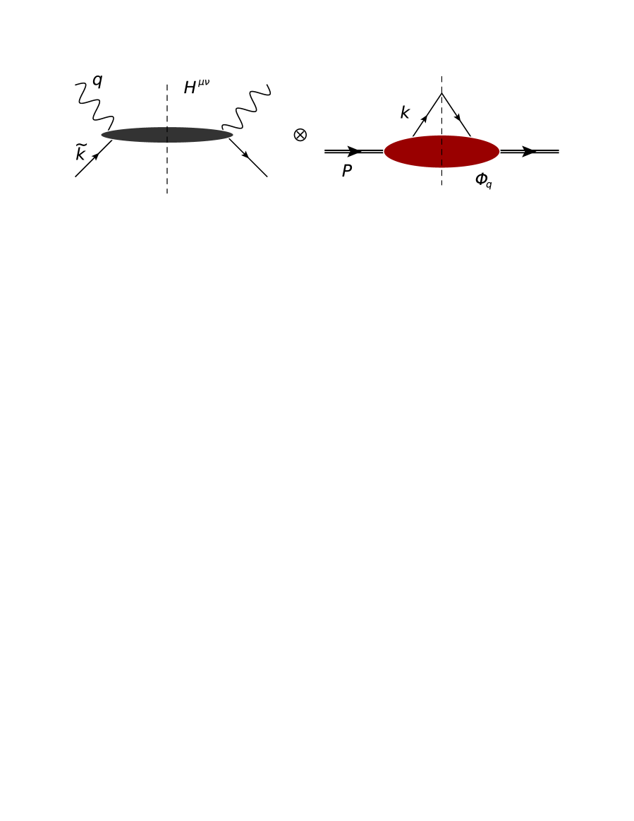
Figure 2: The factorization theorem for the $W_{\mu\nu}$ tensor is the basis of CF formalism applied to inclusive DIS. Here, the hard partonic scattering is represented by the left-hand diagram for $H_{\mu\nu}$, whereas the soft correlators $\Phi_{q}$ encode the nonperturbative dynamics.

Much as we shall illustrate in more formal detail in Sec. 4, the CF paradigm supposes the hadronic tensor of Eq. (1) can be separated in momentum space as

$$W_{\mu\nu}(P,q)\ =\ \sum_{q}\int{dx\over x}\ H^{q}_{\mu\nu}(\tilde{k},q)\cdot\Phi_{q}(x,Q^{2},M^{2})\ +\ \mathcal{O}(1/Q^{2})\ ,$$ (16)

where the sum is over quark flavors and the hard amplitude $H^{q}_{\mu\nu}$ and quark correlator $\Phi_{q}$ of Eq. (21) appear explicitly in Fig. 2. This factorized form is obtained by expanding the quark 4-momenta in the collinear “DIS frame”

$$P^{\mu} = P^{+}\,{\overline{n}}^{\mu}+\frac{M^{2}}{2P^{+}}\,n^{\mu}\ ,$$ (17a)

$$q^{\mu} = -\xi P^{+}\,{\overline{n}}^{\mu}+\frac{Q^{2}}{2\xi P^{+}}\,n^{\mu}\ ,$$ (17b)

$$k^{\mu} = xP^{+}\,{\overline{n}}^{\mu}+\frac{k^{2}+k^{2}_{\perp}}{2xP^{+}}\,n^{\mu}+{\bf k}_{\perp}^{\,\mu}\ ,$$ (17c)

about $\tilde{k}^{\mu}=xP^{+}n^{\mu}$. Roughly speaking, the mass-corrected structure functions can then be projected [135] from the tensor $H^{q}_{\mu\nu}$ using the fact that $F_{i}(x)=h^{q}_{i}\otimes\Phi_{q}(\xi)$, and noting that the $h_{i}$ are parton-level analogues of the helicity structure functions $F_{i}(x)$

Ellis, Furmanski and Petronzio

The first study of TMCs within CF was made by Ellis, Furmanski, and Petronzio (EFP) [132], who analyzed the virtual photon-hadron scattering amplitude using a Feynman diagram technique to expand the hard scattering term about the collinear direction, incorporating both parton off-shellness (or interactions) and parton transverse momentum in twist-4 contributions [143]; this is in contrast to the logic we just sketched, which was kept strictly to twist-2 for simplicity. Using the same notation as for the OPE TMCs above, the EFP results for the target mass corrected structure functions are given by

$$F_{1}^{\rm EFP}(x,Q^{2}) = \frac{2}{1+\rho}F_{1}^{(0)}(\xi,Q^{2})+\frac{(\rho^{2}-1)}{(1+\rho)^{2}}h_{2}(\xi,Q^{2})\,,$$ (18a)

$$F_{2}^{\rm EFP}(x,Q^{2}) = \frac{1}{\rho^{2}}F_{2}^{(0)}(\xi,Q^{2})+\frac{3\xi(\rho^{2}-1)}{\rho^{2}(1+\rho)}h_{2}(\xi,Q^{2})\,,$$ (18b)

$$F_{L}^{\rm EFP}(x,Q^{2}) = F_{L}^{(0)}(\xi,Q^{2})+\frac{2\xi(\rho^{2}-1)}{(1+\rho)}h_{2}(\xi,Q^{2})\,,$$ (18c)

$$F_{3}^{\rm EFP}(x,Q^{2}) = \frac{1}{\rho}F_{3}^{(0)}(\xi,Q^{2})+\frac{2(\rho^{2}-1)}{\rho(1+\rho)^{2}}h_{3}(\xi,Q^{2})\,,$$ (18d)

where again the $F_{i}^{(0)}$ refer to the uncorrected structure functions, and $h_{2,3}$ are given in Eqs. (12). (Note that the definition of the longitudinal structure function in EFP differs from the usual definition (2) by a factor $x$, and the $F_{2}$ structure function is proportional to what EFP call the “transverse” structure function, which in standard usage is proportional to $F_{1}$.) Because the massless functions $F_{i}^{(0)}$ are evaluated at $\xi$, the target mass corrected structure functions will suffer from the same threshold problem as in the OPE analysis in Eqs. (10). While the expressions in Eqs. (18) were derived in Ref. [132] at leading order in $\alpha_{s}$, in this work we will assume their validity also at NLO.

The prefactors for the leading terms proportional to $F_{i}^{(0)}$ in Eqs. (18) are remarkably close to those for the leading terms in the OPE expressions in Eqs. (10). To first order in $1/Q^{2}$, the leading term prefactors for $F_{1}$ in both OPE and EFP reduce to $(1-x^{2}M^{2}/Q^{2})$. Similarly, the $F_{2}$ prefactors both reduce to $(1-4x^{2}M^{2}/Q^{2})$, while those for $F_{L}$ reduce to 1. For the $F_{3}$ structure function, however, the ${\cal O}(1/Q^{2})$ prefactor is $(1-3x^{2}M^{2}/Q^{2})$ for OPE, whereas for the EFP CF result it is $(1-2x^{2}M^{2}/Q^{2})$.

At leading order in the massless limit the longitudinal structure function vanishes identically. At NLO, however, it receives contributions from both quark and gluon PDFs convoluted with the respective hard coefficient functions. For electromagnetic scattering, for example, one has [144, 145]

$$F_{L}^{\gamma(0)}(x,Q^{2})={\alpha_{s}(Q^{2})\over\pi}\int_{x}^{1}{dy\over y}\left({x\over y}\right)^{2}\left\{{4\over 3}F_{2}^{\gamma(0),\rm LO}(y,Q^{2})+c^{\gamma}(y-x)g(y,Q^{2})\right\},$$ (19)

where $c^{\gamma}=2\sum_{q}e_{q}^{2}$, and $F_{2}^{\gamma(0),\rm LO}$ is given by the leading order expression for $F_{2}^{\gamma(0)}$. Similar expressions hold also for the longitudinal structure functions associated with other electroweak currents. In our numerical calculations discussed below we will always compute $F_{L}$ at NLO, which serves as an input to determinations of the phenomenological $R$ ratios and PVDIS asymmetries.

It is important also to note that Eqs. (18) have been derived considering Feynman diagrams with 2 or 4 legs attached to the hadronic correlator (see Figs. 2 and 3 of Ref. [132]), which for $M=0$ give rise to twist-2 and twist-4 contributions to the structure functions, respectively. For $M\neq 0$, however, the quark and gluon equations of motion allow one to extract a twist-2 contribution from the 4-leg diagrams, which when added to the twist-2 target mass correction yields the full result in Eqs. (18). It is an interesting question whether by resumming the twist-2 parts of $n$-leg diagrams one would be able to recover the TMC expressions (18).

Accardi and Qiu

In both the EFP and OPE treatments of TMCs, the resulting structure functions are nonzero for $x>1$. The analysis of Accardi and Qiu (AQ) [135] traced this problem to baryon number nonconservation in the handbag diagram for $M\neq 0$. Working with 2-leg diagrams only, in contrast to EFP who also consider 4-leg diagrams up to twist-4, the AQ target mass corrected structure functions are given by [135]

$$F_{1}^{\rm AQ}(x,Q^{2}) = \widetilde{F}_{1}^{(0)}(\xi,Q^{2}),$$ (20a)

$$F_{2}^{\rm AQ}(x,Q^{2}) = \frac{1+\rho}{2\rho^{2}}\widetilde{F}_{2}^{(0)}(\xi,Q^{2}),$$ (20b)

$$F_{L}^{\rm AQ}(x,Q^{2}) = \frac{1+\rho}{2}\widetilde{F}_{L}^{(0)}(\xi,Q^{2}),$$ (20c)

$$F_{3}^{\rm AQ}(x,Q^{2}) = \frac{1}{\rho}\widetilde{F}_{3}^{(0)}(\xi,Q^{2}).$$ (20d)

Here the functions $\widetilde{F}_{i}^{(0)}$ are defined as

$$\widetilde{F}_{i}^{(0)}(\xi,Q^{2})=\sum_{f}\int_{\xi}^{\xi/x}\!\frac{dz}{z}\,C_{i}^{f}\left({\xi\over z},Q^{2}\right)\varphi_{f}(z,Q^{2}),$$ (21)

where $C_{i}^{f}$ are the perturbatively calculable hard coefficient functions for a given parton flavor $f$, including parton charge factors, $\varphi_{f}$ are the parton densities of the nucleon, and the sum is taken over all active flavors. The upper limit in Eq. (21) ensures that the target mass corrected structure functions vanish for $x>1$, as required by kinematics, although jet mass corrections need to be introduced in order to render the target mass corrected functions zero at $x=1$ [135]. It remains an interesting exercise to apply the same prescription to twist-4 diagrams as in Ref. [132] in order to establish a more direct correspondence between the AQ and EFP approaches. Of course, for $M^{2}/Q^{2}\to 0$ the upper limit of integration in Eq. (21) is 1, and both approaches recover the standard factorization theorem for structure functions [146].

$\xi$-scaling

When the upper limit of integration in Eq. (21) is taken to be 1, the AQ structure functions reduce to the simple $\xi$-scaling ($\xi$-S) form introduced by Aivazis et al. [133] and used by Kretzer and Reno [134]. The target mass corrected structure functions in this case are simply given by

$$F_{1}^{\rm\xi\mbox{-}S}(x,Q^{2}) = F_{1}^{(0)}(\xi,Q^{2})\,,$$ (22a)

$$F_{2}^{\rm\xi\mbox{-}S}(x,Q^{2}) = \frac{1+\rho}{2\rho^{2}}\ F_{2}^{(0)}(\xi,Q^{2})\,,$$ (22b)

$$F_{L}^{\rm\xi\mbox{-}S}(x,Q^{2}) = \frac{1+\rho}{2}F_{L}^{(0)}(\xi,Q^{2})\,,$$ (22c)

$$F_{3}^{\rm\xi\mbox{-}S}(x,Q^{2}) = \frac{1}{\rho}F_{3}^{(0)}(\xi,Q^{2})\,.$$ (22d)

Note that the form of the target mass corrected functions in Eqs. (22) closely resembles that in Eqs. (20), with the two forms equivalent at leading order. At this order the structure functions satisfy a modified Callan-Gross relation [135],

$$\rho^{2}\,F_{2}^{\rm\xi\mbox{-}S}(x,Q^{2})=2xF_{1}^{\rm\xi\mbox{-}S}(x,Q^{2})\,.$$ (23)

The leading order $\xi$-scaling structure functions are also related to the leading, ${\cal O}(1)$ terms of the OPE expressions in Eqs. (10),

$$F_{i}^{\rm OPE\,(leading)}(\xi,Q^{2})=\frac{1+\rho}{2\rho}\ F_{i}^{\rm\xi\mbox{-}S}(\xi,Q^{2})\,,$$ (24)

where the prefactor, to order $1/Q^{2}$, is given by $(1-x^{2}M^{2}/Q^{2})$. In fact, the $\xi$-scaling formulas (22) would coincide with the EFP results in Sec. 2 in the absence of 4-leg Feynman diagrams [132].

3 TMC comparisons

The effects of the different TMC prescriptions on the $F_{2}^{\gamma}$ structure function are illustrated in Fig. 3 as a stand-in for the analogous calculation for other quark flavor combinations and exchange bosons as collected exhaustively in [129].

The uncorrected proton structure function $F_{2}^{(0)}$ (and others required to compute parity-violating asymmetries, etc.) is constructed from the CTEQ-Jefferson Lab (CJ) global PDF fits [122], evaluated at $Q^{2}=2$ GeV². For each of the structure functions the effects of TMCs become more prominent with increasing $x$, and naturally their magnitude decreases at larger $Q^{2}$.

Figure 3: Ratio of target mass corrected to uncorrected (left) or to OPE (right) $F_{2}^{\gamma}$ proton structure functions at $Q^{2}=2$ GeV² for the OPE (solid, red), EFP (short-dashed, blue), $\xi\mbox{-S}$ (long-dashed, green), and AQ (dot-dashed, orange) TMC prescriptions.

For $F_{2}^{\gamma}$ as given in Fig. 3, a dip in the ratio of corrected to uncorrected functions at $x\sim 0.4$, however, delays the sharp rise above unity to $x\gtrsim 0.6$. More pointedly, the EFP result agrees with the OPE to a few percent over the entire $x$ range, and the AQ and $\xi$-scaling ratios are almost identical for $x<0.4$. The two sets of ratios differ by $\lesssim 7\%$ for $x\lesssim 0.7$, before diverging somewhat as $x\to 1$.

3 Implications for Observables

Having examined the differences between the various TMC prescriptions in $F_{2}^{\gamma}$ as an example, in the current section we consider the effects of TMCs, and in particular their model dependence, on several observables that will be measured in upcoming experiments. We train special focus upon the longitudinal to transverse (LT) cross section ratios, as well as the parity-violating deep-inelastic scattering asymmetries for the proton and deuteron, given their prominence in Chap. 2.

1 $R=\sigma_{L}/\sigma_{T}$ ratios

Given the importance of its phenomenology to the general control over the asymmetry $A^{PV}$ of Chap. 2, we first consider mass effects in the cross section ratio $R^{\gamma N}$. The effects of TMCs on the LT ratio are also important in connection with establishing the low-$Q^{2}$ behavior of $R^{\gamma N}$ at finite $x$, so as to determine the onset of gauge invariance constraints on the longitudinal structure function [147].

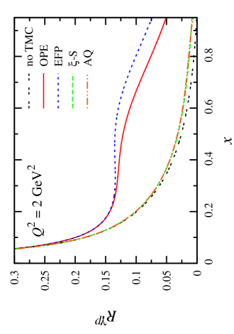
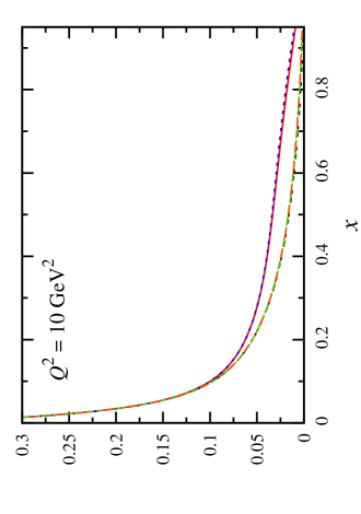
Figure 4: Longitudinal to transverse cross section ratio $R^{\gamma p}$ for the proton at $Q^{2}=2$ GeV² (left) and $Q^{2}=10$ GeV² (right), for no TMCs (double-dashed, black), the OPE (solid, red), EFP (short-dashed, blue), $\xi$-S (long-dashed, green), and AQ (dot-dashed, orange) TMC prescriptions.

In Fig. 4 we illustrate the TMC effects on $R^{\gamma p}$ for $Q^{2}=2$ and 10 GeV² for each of the TMC prescriptions considered in Sec. 2. All of the TMCs increase the magnitude of the $R^{\gamma p}$ ratio, with the AQ and $\xi$-S prescriptions having a relatively modest effect (approximately a factor 2 for $x\approx 0.6-0.8$ at $Q^{2}=2$ GeV², but only a few percent at $Q^{2}=10$ GeV²), whereas the EFP and OPE both modify the ratio significantly for $x\gtrsim 0.1$. The enhancement of $R^{\gamma p}$ for the latter is predicted to be about an order of magnitude for $x\approx 0.6-0.8$ at $Q^{2}=2$ GeV², and still a factor of $3-4$ at $Q^{2}=10$ GeV².

Some differences are also expected between the longitudinal to transverse cross section ratios at NLO for processes involving electromagnetic and weak currents. In particular, we have already quantified in Chap. 2 the fact that asymmetries measured in parity-violating electron scattering are sensitive to interference effects between $\gamma$ and $Z$ boson exchange, and differences between the $R^{\gamma}$ and $R^{\gamma Z}$ LT ratios can affect the measured asymmetries [66, 136].

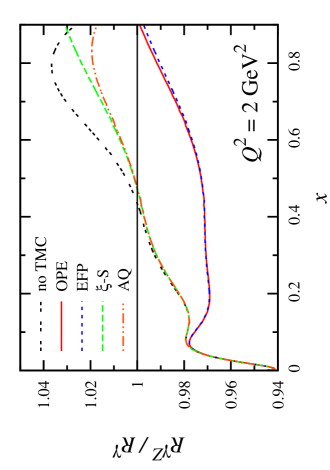
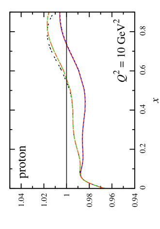
Figure 5: Ratio of $R^{\gamma Z}$ to $R^{\gamma}$ LT ratios for the proton computed at NLO for $Q^{2}=2$ GeV² (left) and $Q^{2}=10$ GeV² (right), for no TMCs (double-dashed, black), the OPE (solid, red), EFP (short-dashed, blue), $\xi$-S (long-dashed, green), and AQ (dot-dashed, orange) TMC prescriptions.

In Fig. 5 the ratio of the proton $R^{\gamma Z}$ to $R^{\gamma}$ LT ratios is shown at $Q^{2}=2$ and 10 GeV². While at leading order both of these ratios are zero, at NLO the different relative contributions from quark PDFs to the electromagnetic and $\gamma Z$ interference structure functions leads to deviations of the ratios from unity of up to $\approx 4\%$ at $Q^{2}=2$ GeV², and up to $\approx 2\%$ at $Q^{2}=10$ GeV². The effects of the TMCs are again very small for the $\xi$-scaling and AQ prescriptions, but more significant for the OPE and EFP results. Overall, the spread in the TMC predictions for the $R^{\gamma Z}/R^{\gamma}$ ratio amounts to $\lesssim 4-5\%$ for $x$ between 0.6 and 0.8 at $Q^{2}=2$ GeV², and $\lesssim 2\%$ at $Q^{2}=10$ GeV². Note that the dip in the ratios at $x<0.1$, which is insensitive to TMCs, reflects the greater role played by gluons at low $x$, but is mostly irrelevant for the kinematics of typical proposed experiments [124, 125, 126], and also more peripheral with regard to signals of nonperturbative physics in the high $x$ valence region.

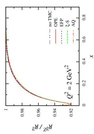
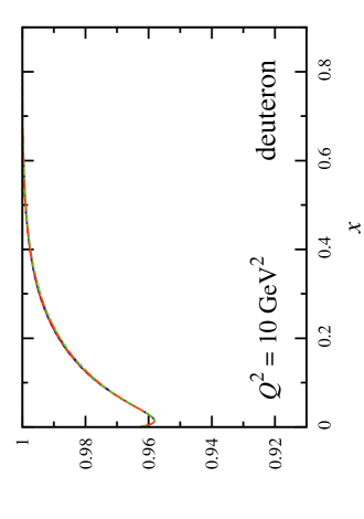
Figure 6: As in Fig. 5, but for the deuteron $R^{\gamma Z}$ to $R^{\gamma}$ LT ratio.

For the case of the isoscalar deuteron target, stronger cancellations between the quark content of $R^{\gamma Z}$ and $R^{\gamma}$ are expected to lead to smaller deviations of their ratio from unity at large $x$; this is perhaps unsurprising given a similar dampening of the finite-$Q^{2}$ effects relative to the proton as we observed in Figs. 9 & 8. This behavior is indeed observed again in Fig. 6, where, much like like Fig. 5, the dip in the ratio at very low $x$ is associated with NLO gluon dominance of the LT ratios as $x\to 0$. At $x=0.2$, for example, the gluonic content of $F_{L}$ suppresses the deuteron $R^{\gamma Z}/R^{\gamma}$ ratio by $\approx 2\%$ for $Q^{2}=2$ GeV², and $\approx 1\%$ for $Q^{2}=10$ GeV². At higher $x$ the deviations decrease until the ratio approaches unity asymptotically as $x\to 1$. In the region of $x$ where the LT ratios are dominated by quarks, the fact that the same isoscalar combination of quark PDFs enters both the electromagnetic and $\gamma Z$ interference structure functions leads to almost negligible TMC effects. The absence of significant TMC effects in the deuteron ratio is, as expected, even more clearly visible at the higher $Q^{2}$ value.

2 PVDIS asymmetries

In this section we examine the effects of TMCs on the PVDIS asymmetries of the proton and deuteron, and discuss the phenomenological implications of their uncertainties on future planned experiments.

Proton asymmetry

The proton PVDIS asymmetry is shown in Fig. 7 for $Q^{2}=2$ and 10 GeV² in the form of the ratio of the target mass corrected to uncorrected asymmetries. For all prescriptions the TMC effects are maximal at $x\approx 0.7$, where they are of the order of $3-4\%$ at $Q^{2}=2$ GeV² and $\lesssim 1\%$ at $Q^{2}=10$ GeV². The results are slightly higher for the $\xi$-S and AQ corrections (which are virtually indistinguishable) than for the OPE and EFP (which are also almost identical). The small size of the effects is principally due to the strong cancellation of the TMCs in the $F_{1}$ structure functions [effectively, the hadronic-vector part of $A^{PV}$ in Eq. (33)], namely, $(F_{1}^{\gamma Z}/F_{1}^{\gamma})^{\rm TMC}\approx(F_{1}^{\gamma Z}/F_{1}^{\gamma})^{(0)}$, even though $|F_{1}^{\rm TMC}/F_{1}^{(0)}|\gg 1$ at high $x$. Overall, the results indicate that the asymmetries themselves are less sensitive to TMCs than are the LT ratios $R^{\gamma,\gamma Z}$ on which the asymmetries depend.

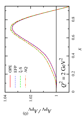
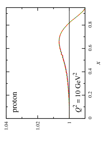
Figure 7: Ratio of target mass corrected ($A_{\rm PV}$) to uncorrected ($A_{\rm PV}^{(0)}$) PVDIS asymmetries for the proton at $Q^{2}=2$ GeV² (left) and $Q^{2}=10$ GeV² (right), for the OPE (solid, red), EFP (short-dashed, blue), $\xi$-S (long-dashed, green), and AQ (dot-dashed, orange) TMC prescriptions. Note that the AQ and $\xi$-S results are almost indistinguishable, as are the EFP and OPE prescriptions.

Since one of the main goals of the proton PVDIS measurements will be to reduce the uncertainties on PDFs at large $x$, particularly on the $d/u$ ratio, it is instructive to compare the magnitude of the TMC effects with the expected sensitivity of the asymmetry to different possible PDF behaviors at large $x$. In Fig. 8 we show the proton asymmetry $A_{\rm PV}$ computed from the full range of CJ PDFs [122] including minimal and maximal nuclear corrections (shaded bands) relative to the central PDF fits. The uncertainty band increases with increasing $x$, reflecting the larger uncertainty on the $d$ quark PDF at large $x$, and in the absence of TMCs ranges from $\approx 3\%$ at $x=0.6$ to $\approx 11\%$ at $x=0.8$ for both $Q^{2}=2$ and 10 GeV². This is significantly larger than the TMC uncertainty band in Fig. 7, where the spread of the TMC model predictions is $\ll 1\%$, even though the absolute target mass effect is somewhat larger.

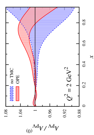
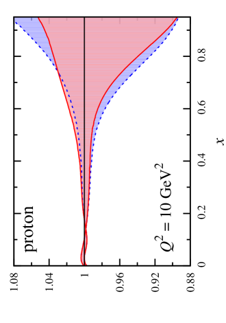
Figure 8: Proton PVDIS asymmetry $A_{\rm PV}$ at $Q^{2}=2$ GeV² (left) and $Q^{2}=10$ GeV² (right) for CJ PDFs with minimal and maximal nuclear effects [122] (shaded bands), relative to the asymmetry $A_{\rm PV}^{(0)}$ for the central CJ PDF fits, with no TMCs (dashed, blue) and using the OPE TMC prescription (solid, red).

The effect of TMCs on the PDF uncertainty, illustrated in Fig. 8 for the OPE prescription, is to reduce the uncertainty band at large $x$ for the lower $Q^{2}$ value, with strength resultingly moving from lower $x$ to higher $x$ by the $x\to\xi$ rescaling of the structure functions. The slightly different effects of TMCs on the various structure functions present in the asymmetry render the uncertainty band on $A_{\rm PV}$ more asymmetric at $Q^{2}=2$ GeV². At the higher $Q^{2}=10$ GeV² value, the impact of TMCs on the uncertainty band is reduced considerably, with the two bands (corresponding to no TMCs and the OPE TMC prescription) approximately coinciding for all $x$.

The conclusion from the combined results of Figs. 7 and 8 is that the effect of TMCs and particularly their uncertainties can be minimized in the $A_{\rm PV}$ ratio by measuring the asymmetry at values of $Q^{2}\sim 10$ GeV² or higher; at lower $Q^{2}$, although the TMC uncertainties are not large, some residual corrections will need to be applied in the range $0.4\lesssim x\lesssim 0.9$, where the TMCs are $\approx 1\%$ or higher.

Deuteron asymmetry

As we witnessed in Chap. 2, PVDIS on an isoscalar deuterium nucleus features a near total cancellation of the dependence on PDFs if charge symmetry is strictly assumed [137]. In fact, it is convenient for our purposes here to recast the valence quark region ($x\gtrsim 0.5$) deuteron asymmetry of Eq. (45) at leading order as

$$A_{\rm PV}^{d}\ \approx\ -\left({G_{F}Q^{2}\over 2\sqrt{2}\pi\alpha}\right){6\over 5}\left(g_{A}^{e}(2g_{V}^{u}-g_{V}^{d})\ +\ Y_{3}\,g_{V}^{e}(2g_{A}^{u}-g_{A}^{d})\right)\ ,\ \ \ \ \ \ [x\gg 0]\ ,$$ (25)

where the couplings $g_{V}^{u,d}$, etc., are again specified by Eq. (15) of Chap. 2. We have seen that accurate measurement of deuteron PVDIS is thus a potentially sensitive test of either the weak mixing angle $\sin^{2}\theta_{W}$ (deviations of which from its Standard Model value may signal the presence of new physics), or more conventionally, of charge symmetry violation (CSV) in PDFs.

We have also argued that nonzero values of $\delta u$ and $\delta d$ are predicted in various nonperturbative models of the nucleon to arise from quark mass differences and electromagnetic effects, and can also be generated from radiative QED corrections in $Q^{2}$ evolution [80, 81, 82] as we simulated in Chap. 2.3. If we again define charge symmetry violating PDFs by

$$\delta u=u^{p}-d^{n}\ ,\ \ \ \ \ \ \delta d=d^{p}-u^{n}\ ,$$ (26)

the PVDIS asymmetry (25) in the presence of CSV is modified according to

$$(2g_{V,A}^{u}-g_{V,A}^{d}) \to (2g_{V,A}^{u}-g_{V,A}^{d})(1+\Delta_{V,A})\ ,$$ (27)

where the fractional CSV corrections are given by

$$\Delta_{V,A} = \left(-\frac{3}{10}+\frac{2g_{V,A}^{u}+g_{V,A}^{d}}{2(2g_{V,A}^{u}-g_{V,A}^{d})}\right)\left(\frac{\delta u-\delta d}{u+d}\right)\ .$$ (28)

These approximate expressions serve to illustrate explicitly the role of CSV in the PVDIS asymmetry in a fashion that explicitly manifests the vector/axial-vector structure of Eq. (10), for example; in practice, however, the full deuteron asymmetry can be computed including the effects of CSV at NLO, as well as sea quarks and gluons.

Using the MRSTQED parametrization of PDFs [81] similar to our description in Sec. 2, we illustrate the effect of CSV on the deuteron asymmetry $A_{\rm PV}^{d}$ in Fig. 9. Deviations of the full NLO result from the valence approximation of Eq. (51) appear already at $x\lesssim 0.7$, and the various CSV treatments differ quite markedly at small $x$, as Fig. 9 indicates. Interestingly, the full asymmetry becomes larger at smaller $x$ because of CSV effects in the light sea quarks, which produce an asymmetry of about 2% at $x\approx 0.2$. On the other hand, cleanly separating the CSV effects from sea quark and gluon contributions, which introduce additional $x$ dependence beyond that in Eqs. (25), (27) and (28), as well as possible differences between CSV in valence and sea quark PDFs, becomes more challenging at small $x$.

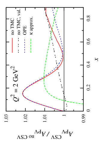
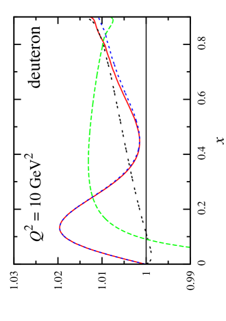
Figure 9: Deuteron PVDIS asymmetry including CSV effects, relative to the asymmetry with charge-symmetric PDFs, at $Q^{2}=2$ GeV² (left) and $Q^{2}=10$ GeV² (right). The CSV PDFs are computed from the MRSTQED parametrization [81] for the full asymmetry (solid, red) and for the valence approximation (double-dashed, black), and from the $\kappa$-dependent fit (see text) in Ref. [80] (long-dashed, green). The effects of TMCs on the full asymmetry with the MRSTQED PDFs are illustrated for the OPE prescription (short-dashed, blue).

With sought-after CSV effects that could be $\lesssim 1-2\%$, it is vital to quantify the impact of TMCs on the deuteron PVDIS asymmetries and in particular the TMC prescription dependence. The effect of TMCs on the full asymmetry relative to the charge-symmetric asymmetry is negligible at $x\lesssim 0.5$, but decreases the CSV signal by up to 50% at $x\approx 0.8$, as Fig. 9 demonstrates for the OPE prescription. The model dependence of the mass corrections is illustrated for the various prescriptions in Fig. 10, wherein we plot the ratio PV asymmetries with and without TMCs. The net effect is very small, peaking at $\sim 0.1\%$ at $x\approx 0.4$, even at the $Q^{2}=2$ GeV² value. The TMC prescription dependence of this ratio is even smaller, making it essentially negligible on the scale of a CSV signal of $\sim 1\%$. If the target mass corrected asymmetries were calculated with the charge symmetry violating MRSTQED PDFs, the effect would be somewhat larger, peaking at $\sim 0.3\%$ around $x\approx 0.4$. However, the TMC model dependence is still negligible at around 0.05%. As expected, the impact of TMCs on the deuteron asymmetries at the larger $Q^{2}=10$ GeV² value is considerably smaller. It is therefore likely that TMCs would only play a role in deuteron PVDIS measurements if the CSV effects were on the scale of a fraction of a percent, at which point they would not be discernible within the expected precision of proposed experiments, e.g., [126].

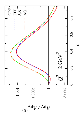
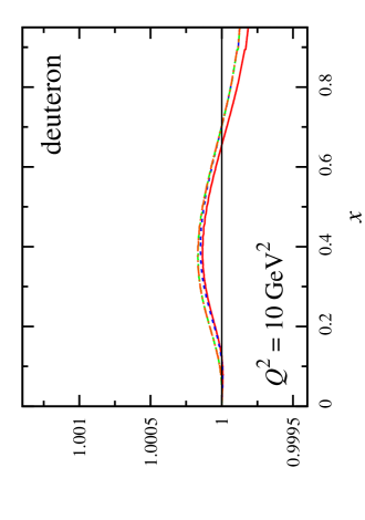
Figure 10: Ratio of target mass corrected to uncorrected PVDIS deuteron asymmetries $A_{\rm PV}^{d}$ at $Q^{2}=2$ GeV² (left) and $Q^{2}=10$ GeV² (right), for the OPE (solid, red), EFP (short-dashed, blue), $\xi$-S (long-dashed, green), and AQ (dot-dashed, orange) TMC prescriptions.

4 Semi-inclusive Hadron Mass Corrections

Having catalogued the physics of mass effects in fully inclusive DIS, we turn our attention to the corresponding treatment of semi-inclusive deep inelastic scattering (SIDIS), which has in recent years received great attention as a tool to investigate various aspects of hadron structure; counted highly among these is the flavor dependence of the nucleon’s parton distribution functions, polarized and unpolarized, which may be assessed through flavor tagging of final state hadrons. Observation of the momentum distribution of produced hadrons also allows access to the largely unexplored transverse momentum dependent parton distributions, which reveal a much richer landscape of the spin and momentum distribution of quarks in the nucleon. This will be made all the clearer by the phenomenological computations of Chap. 5.

At high energies the scattering and hadronization components of the SIDIS process factorize and the cross section can be represented as a product of parton distribution and fragmentation functions. In practice, however, experiments are often carried out at few-GeV energies with $Q^{2}$ as low as 1 GeV², suggesting that $1/Q^{2}$ power corrections must be controlled in order to determine the applicability of partonic analyses of the data. Despite the fairly robust use of the OPE in inclusive scattering we just observed, this method cannot be rigorously extended to the production of hadrons in the final state. This is because hadronic matrix elements in SIDIS are technically off-diagonal, and hence lack the symmetric basis required for expansions of the type given in Eq. (46). Due to their direct formulation in momentum space, collinear factorization techniques, however, can be extended to SIDIS, a fact we demonstrate in the present section.

In contrast to fully inclusive DIS, where the only mass scale entering the problem is that of the target hadron, in SIDIS finite-$Q^{2}$ corrections arise from both the target mass and the mass of the produced hadron. For generality we shall refer to their combined effects as “hadron mass corrections” (HMCs). Accordingly, we use the CF framework to derive the mass corrections to the SIDIS cross section at finite $Q^{2}$, and systematically investigate their implications at kinematics relevant to contemporary experiments. In Sec. 1 – 2 we review the formal aspects of the collinear approach and discuss their application to semi-inclusive hadron production. To expose the origin of the corrections we work at leading order in $\alpha_{s}$.

In Sec. 3 we explore the relative importance of the HMCs numerically, and evaluate the size of the corrections in the cross sections and fragmentation functions at various kinematics. To assess their possible impact on data analyses, we also compare the magnitude of the HMCs at kinematics typical of modern facilities like Jefferson Lab with experimental errors from recent experiments.

1 Collinear kinematics

We begin the discussion of SIDIS at finite values of the photon virtuality $Q^{2}$ by defining the relevant kinematics and momentum variables in a collinear frame, and introduce the hadronic tensor computed in a covariant parton model. Collinear factorization is then performed in the leading order approximation in which the produced hadron is effectively collinear with the scattered parton, which more directly reveals the effects of hadron masses on the cross sections and fragmentation functions.

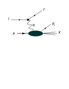
Figure 11: Unlike fully inclusive DIS, some of the hadronic final state is directly observed in SIDIS — in our case, a single produced hadron (e.g., a pion or kaon) of momentum $p_{h}$.

By definition, a collinear frame in Minkowski space is defined by any two 4-vectors. The intersection of the plane where they lie with the light-cone defines the light-cone $4$-vectors ${\overline{n}}^{\mu}$ and $n^{\mu}$, which satisfy $n^{2}={\overline{n}}^{2}=0$ and ${\overline{n}}\cdot n=1$. In SIDIS the hadronic tensor depends on the $4$-vectors $P^{\mu}$, $q^{\mu}$ and $p_{h}^{\mu}$ that in turn define three possible collinear frames denoted $(P,q)$, $(p_{h},q)$ and $(p_{h},P)$. More pointedly, these correspond to the $4$-momenta of the struck nucleon $(P)$, virtual exchange photon $(q)$, and final state, or ‘produced,’ hadron $(p_{h})$; the basic relationship among these parameters is illustrated schematically in Fig. 11.

The $(P,q)$ frame is the only frame that can be defined in DIS and is the one used in this work; the $(p_{h},q)$ frame on the other hand is unique to semi-inclusive hadron production in $e^{+}e^{-}$ collisions; and finally the $(p_{h},P)$ frame is typically preferred for analysis of transverse momentum dependent parton distributions in SIDIS.

In terms of the vectors $P$, $q$ and $p_{h}$ one can define two fragmentation invariants,

$$z_{h} =\frac{P\cdot p_{h}}{P\cdot q}\ ,\qquad\eta_{h}=\frac{2p_{h}\cdot q}{q^{2}}\,,$$ (29)

which together with $x_{B}$, $Q^{2}$, $M^{2}$ and $m_{h}^{2}$ form a complete set of scalar Lorentz invariants in SIDIS. Note that for the purposes of the present section, we refer to the Bjorken limit parameter $x$ of previous chapters as $x_{B}$, so as to prevent confusion with an analogous parton-level variable to be introduced shortly. Because the variable $\eta_{h}$ is defined independently of the target momentum, the effects of the final state hadron mass will decouple from those of the target mass in all reference frames. In contrast, $z_{h}$ is defined in terms of both the target and produced hadron momenta, so that the target and hadron mass effects here will be entangled.

The light-cone fractional momentum $\xi$ (Nachtmann variable) and the fragmentation variable $\zeta_{h}$ are defined in terms of the plus and minus components of the momenta as

$$\xi=-\frac{q^{+}}{P^{+}}\ ,\qquad\zeta_{h}=\frac{p_{h}^{-}}{q^{-}}\ .$$ (30)

We use these definitions in all three frames; however, in each frame the light-cone vectors (and therefore the plus and minus components of the 4-momenta) will be different. In the following we discuss each of the three collinear frames and the consequences within each frame of the choice of fragmentation invariant.

In the DIS frame $(P,q)$ used to compute in subsequent sections, the 4-momenta of the target nucleon ($P$), virtual photon ($q$) and produced hadron $h$ ($p_{h}$) can be decomposed in terms of light-cone unit vectors $n$ and ${\overline{n}}$ as [156]

$$P^{\mu} = P^{+}\,{\overline{n}}^{\mu}+\frac{M^{2}}{2P^{+}}\,n^{\mu}\ ,$$ (31a)

$$q^{\mu} = -\xi P^{+}\,{\overline{n}}^{\mu}+\frac{Q^{2}}{2\xi P^{+}}\,n^{\mu}\ ,$$ (31b)

$$p_{h}^{\mu} = \frac{\xi m_{h\perp}^{2}}{\zeta_{h}Q^{2}}P^{+}\,{\overline{n}}^{\mu}+\frac{\zeta_{h}Q^{2}}{2\xi P^{+}}\,n^{\mu}+p_{h\perp}^{\,\mu}\ ,$$ (31c)

where as usual $M$ is the target nucleon mass, $Q^{2}=-q^{2}$, and the light-cone vectors satisfy $n^{2}={\overline{n}}^{2}=0$ and $n\cdot{\overline{n}}=1$. Here we define light-cone components of any 4-vector $v$ by $v^{+}=v\cdot{\overline{n}}=(v_{0}+v_{z})/\sqrt{2}$ and $v^{-}=v\cdot n=(v_{0}-v_{z})/\sqrt{2}$. The momenta $P$ and $q$ are chosen to lie in the same plane as $n$ and ${\overline{n}}$; particularly advantageous for the analysis of inclusive DIS, we designate this the $(P,q)$ collinear frame.

The nucleon plus-momentum $P^{+}$ can be interpreted as a parameter for boosts along the $z$-axis, connecting the target rest frame to the infinite-momentum frame; the target rest frame ($P^{+}=M/\sqrt{2}$) and the Breit frame ($P^{+}=Q/(\sqrt{2}\xi$)) are part of this family of frames. The transverse momentum 4-vector of the produced hadron $p_{h\perp}^{\,\mu}$ satisfies $p_{h\perp}\cdot n=p_{h\perp}\cdot{\overline{n}}=0$, and we define the transverse mass squared as $m_{h\perp}^{2}=m_{h}^{2}-p_{h\perp}^{2}$, where $m_{h}$ is the produced hadron mass, and the transverse 4-vector squared is $p_{h\perp}^{2}=-\bm{p}_{h\perp}^{\,2}$.

In the chosen collinear frame the variable $\xi=-q^{+}/P^{+}$ defined in Eq. (31b) coincides with the finite-$Q^{2}$ Nachtmann scaling variable [153, 162],

$$\xi=\frac{2x_{B}}{1+\sqrt{1+4x_{B}^{2}M^{2}/Q^{2}}}\ ,$$ (32)

which in the Bjorken limit ($Q^{2}\to\infty$ at fixed $x_{B}$) reduces to the Bjorken scaling variable $x_{B}=Q^{2}/2P\cdot q$. The scaling fragmentation variable $\zeta_{h}=p_{h}^{-}/q^{-}$ defined in Eq. (31c) is related to the fragmentation invariant $z_{h}=P\cdot p_{h}/P\cdot q$ by

$$\zeta_{h} =\frac{z_{h}}{2}\frac{\xi}{x_{B}}\left(1+\sqrt{1-\frac{4x_{B}^{2}M^{2}m_{h\perp}^{2}}{z_{h}^{2}\ Q^{4}}}\right)\,,$$ (33a)

and the positivity of the argument in the radical in Eq. (33a) is ensured by the condition $$E_{h}\geq m_{h\perp}$$, which imposes

$$z_{h}\geq z_{h}^{\rm min}=2x_{B}\frac{Mm_{h}}{Q^{2}}\ .$$ (33b)

One can also define $$\zeta_{h} \eta_{h}=2p_{h}\cdot q/q^{2}$$ in terms of the invariant by

$$\zeta_{h} =\frac{\eta_{h}}{2}\left(1+\sqrt{1+\frac{4m_{h\perp}^{2}}{\eta_{h}^{2}\ Q^{2}}}\right)\ ,$$ (33c)

which is convenient for discriminating between the target and current fragmentation hemispheres in hadron production. Note that in the target rest frame $z_{h}=E_{h}/\nu$ is the usual ratio of the produced hadron to virtual photon energies. In the Breit frame $\eta_{h}=p_{hz}/q_{z}$ is the ratio of the longitudinal components of the hadron and photon energies, which can be used to define the current ($\eta_{h}>0$) and target ($\eta_{h}<0$) hemispheres for hadron production. In the Bjorken limit one has $\zeta_{h}\to z_{h}\to\eta_{h}$.

Conservation of 4-momentum and baryon number impose an upper limit on the $x_{B}$ variable,

$$x_{B}\leq\left(1+{m_{h}^{2}+2Mm_{h}\over Q^{2}}\right)^{-1}\equiv x_{B}^{\rm max}\,,$$ (34)

which corresponds to the exclusive production of a nucleon and a hadron $h$ in the final state. Similarly the limits on the fragmentation variable $\zeta_{h}$ are given by

$$\frac{\xi}{1-\xi}\frac{M^{2}}{Q^{2}}\leq\zeta_{h}\leq 1+\xi\frac{M^{2}}{Q^{2}}\,,$$ (35)

where the lower limit corresponds to diffractive production of the hadron $h$, and the upper limit reflects the fragmentation threshold, which approaches unity in the Bjorken limit.

As mentioned, the $(P,q)$ frame of Eq. (31) is hardly a unique selection, and we might equally well compute in an alternative collinear frame; these choices lead of course to slightly modified scaling parameters, as we summarize here.

For the sake of comparison and completeness, the $(p_{h},q)$ frame used in Ref. [160] defines the external SIDIS vectors as

$$P^{\mu} = P^{+}{\overline{n}}^{\mu}+\frac{M_{\perp}^{2}}{2P^{+}}n^{\mu}+P_{\perp}^{\,\mu}\ ,$$ (36a)

$$q^{\mu} = -\xi P^{+}{\overline{n}}^{\mu}+\frac{Q^{2}}{2\xi P^{+}}n^{\mu}\ ,$$ (36b)

$$p_{h}^{\mu} = \frac{m_{h}^{2}}{\zeta_{h}Q^{2}/\xi}P^{+}{\overline{n}}^{\mu}+\zeta_{h}\frac{Q^{2}}{2\xi P^{+}}n^{\mu}\ ,$$ (36c)

where $M_{\perp}^{2}=M^{2}-P_{\perp}^{2}=M^{2}+\bm{P}_{\perp}^{2}$ is the transverse mass of the target nucleon. The Nachtmann variable in this case is given by

$$\xi=\frac{2x_{B}}{1+\sqrt{1+4x_{B}^{2}M_{\perp}^{2}/Q^{2}}}\ ,$$ (37)

which, in contrast to its definition in the $(P,q)$ frame, depends explicitly on the transverse mass of the target nucleon. Furthermore, in terms of the fragmentation invariant $z_{h}$, the finite-$Q^{2}$ fragmentation variable $\zeta_{h}$ is given by

$$\zeta_{h}=\frac{z_{h}}{2}\frac{\xi}{x_{B}}\left(1+\sqrt{1-4\frac{x_{B}^{2}}{z_{h}^{2}}\frac{M_{\perp}^{2}m_{h}^{2}}{Q^{4}}}\right)\ ,$$ (38)

or in terms of $\eta_{h}$ by

$$\zeta_{h}=\frac{\eta_{h}}{2}\left(1+\sqrt{1+4\frac{1}{\eta_{h}^{2}}\frac{m_{h}^{2}}{Q^{2}}}\right)\ .$$ (39)

Lastly, we point out that the external vectors in the $(p_{h},P)$ frame of Ref. [161] are specified by

$$P^{\mu} = P^{+}{\overline{n}}^{\mu}+\frac{M^{2}}{2P^{+}}n^{\mu}\ ,$$ (40a)

$$q^{\mu} = -\xi P^{+}{\overline{n}}^{\mu}+\frac{Q_{\perp}^{2}}{2\xi P^{+}}n^{\mu}+q_{\perp}^{\,\mu}\ ,$$ (40b)

$$p_{h}^{\mu} = \frac{m_{h}^{2}}{\zeta_{h}Q^{2}/\xi}P^{+}{\overline{n}}^{\mu}+\zeta_{h}\frac{Q^{2}}{2\xi P^{+}}n^{\mu}\ ,$$ (40c)

where $Q_{\perp}^{2}=Q^{2}-q_{\perp}^{2}=Q^{2}+\bm{q}_{\perp}^{2}$ is the transverse mass of the virtual photon. The Nachtmann variable in this frame depends explicitly on $Q_{\perp}^{2}$,

$$\xi=\frac{Q_{\perp}^{2}}{Q^{2}}\frac{2x_{B}}{1+\sqrt{1+4x_{B}^{2}M^{2}Q_{\perp}^{2}/Q^{4}}}\ ,$$ (41)

and the finite-$Q^{2}$ fragmentation variable is given by

$$\zeta_{h}=\frac{z_{h}}{2}\frac{\xi}{x_{B}}\frac{Q^{2}}{Q_{\perp}^{2}}\left(1+\sqrt{1-4\frac{x_{B}^{2}}{z_{h}^{2}}\frac{M^{2}m_{h}^{2}}{Q^{4}}}\right)\ ,$$ (42)

or

$$\zeta_{h}=\frac{\eta_{h}}{2}\frac{Q^{2}}{Q_{\perp}^{2}}\left(1+\sqrt{1+\frac{4}{\eta_{h}^{2}}\frac{m_{h}^{2}Q_{\perp}^{2}}{Q^{4}}}\right)\ .$$ (43)

While the three frames discussed here are generally distinct, up to leading order in $1/Q^{2}$ the vectors $P$, $q$ and $p_{h}$ lie in the same plane and the frames actually coincide. Comparing the $(P,q)$ and $(p_{h},q)$ frames, for example, the differences between the transverse momenta and scaling variables can be expressed as

$$\bm{p}_{h\perp} =\bm{P}_{\perp}^{*}+{\cal O}(\bm{P}_{\perp}^{*2}/Q^{2})\,,$$ (44a)

$$\xi =\xi^{*}+{\cal O}(\bm{P}_{\perp}^{*2}/Q^{2})\,,$$ (44b)

$$\zeta_{h} =\zeta_{h}^{*}+{\cal O}(\bm{P}_{\perp}^{*2}/Q^{2})\,,$$ (44c)

where the asterisks (^∗) label quantities in the $(p_{h},q)$ frame. Similar relations are applicable also for the parton fractional momentum $x$ and the hadron fractional momentum $z$. At leading order in collinear factorization one has $\bm{p}_{h\perp}=0$ and the frames are manifestly equivalent. Moreover, since $\langle\bm{p}^{2}_{h\perp}\rangle\ll Q^{2}$ for $\bm{p}_{h\perp}$-integrated cross sections at next-to-leading order the differences between the collinear frames should remain small. For the sake of future work, it will be important to check more thoroughly whether, and in what kinematic range, this approximation is valid; this is especially true for unintegrated cross sections, where differences between frames become relevant and must be better quantified.

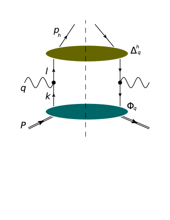
Figure 12: Parton-level kinematics of semi-inclusive deep inelastic lepton–nucleon scattering at leading order, producing a final state hadron $h$. The momenta of the target nucleon ($P$), virtual photon ($q$), incident ($k$) and scattered quarks ($l$), and the produced hadron ($p_{h}$) are labeled explicitly, with $\Phi_{q}$ and $\Delta^{h}_{q}$ denoting the correlators relevant to the quark distribution and fragmentation functions. The vertical dashed line represents the cut of the forward amplitude.

Parton kinematics in collinear factorization.

Having charted formal issues related to frame choices, we proceed with the analysis using the decomposition in the $(P,q)$ frame of Eq. (31). At the partonic level the SIDIS process at leading order in $\alpha_{s}$ is illustrated in Fig. 12. It occurs by means of scattering from a quark carrying a light-cone momentum fraction $x=k^{+}/P^{+}$, which then fragments (nonperturbatively) to a hadron $h$ carrying a light-cone momentum fraction $z=p_{h}^{-}/l^{-}$, where $k$ and $l$ are the 4-momenta of the initial and scattered quarks. At higher orders the hard scattering can also take place from a gluon, and additional partons might be created in the collision.

The parton momenta $k$ and $l$ can be parametrized in terms of the light-cone vectors $n$ and ${\overline{n}}$ as

$$k^{\mu} = xP^{+}\,\bar{n}^{\mu}+\frac{k^{2}+k_{\perp}^{2}}{2xP^{+}}\,n^{\mu}+k_{\perp}^{\mu}\ ,$$ (45a)

$$l^{\mu} = \frac{l^{2}+l_{\perp}^{2}}{2p_{h}^{-}/z}\,\bar{n}^{\mu}+\frac{p_{h}^{-}}{z}\,n^{\mu}+l_{\perp}^{\mu}\ ,$$ (45b)

with the parton transverse momentum 4-vectors $k_{\perp}$ and $l_{\perp}$ orthogonal to $n$ and ${\overline{n}}$. In collinear factorization the hard scattering amplitude is expanded around on-shell and collinear momenta $\tilde{k}$ and $\tilde{l}$,

$$\tilde{k}^{\mu} = xP^{+}\,\bar{n}^{\mu}+\frac{\tilde{k}^{2}}{2xP^{+}}\,n^{\mu}\,$$ (46a)

$$\tilde{l}^{\mu} = \frac{\tilde{l}^{2}+p_{h\perp}^{2}/z^{2}}{2p_{h}^{-}/z}\,\bar{n}^{\mu}+{p_{h}^{-}\over z}\,n^{\mu}+{p_{h\perp}^{\mu}\over z}\ ,$$ (46b)

where the initial and final collinear parton “masses” $\tilde{k}^{2}$ and $\tilde{l}^{2}$ are kept for generality.

Defining the invariant $\hat{x}=-q^{2}/2\tilde{k}\cdot q$ as the partonic analog of the Bjorken variable $x_{B}$, at finite $Q^{2}$ one has

$$\hat{x}={\xi\over x}\left(1+{x\over\xi}{\tilde{k}^{2}\over Q^{2}}\right)\,.$$ (47)

Using the formal methods of Ref. [159] one can show that for SIDIS cross sections integrated over $p_{h\perp}$, $\hat{x}$ is constrained to be in the range

$$1+\frac{m_{h}^{2}}{\zeta_{h}Q^{2}}-\frac{\tilde{k}^{2}}{Q^{2}}\left(1-\frac{\xi m_{h}^{2}}{x\zeta_{h}Q^{2}}\right)\leq\,\frac{1}{\,\hat{x}\,}\,\leq\frac{1}{x_{B}}\left(1-x_{B}\frac{2Mm_{h}+\tilde{k}^{2}}{Q^{2}}\right)\ ,$$ (48)

where the lower limit arises from the minimum of the current jet mass, and the upper limit corresponds to collinear spectators with minimal mass. These limits agree with the limit on $x_{B}$ in Eq. (34) for any $\tilde{k}^{2}\geq x(\zeta_{h}-1)Q^{2}/\xi$. For the fragmentation process one finds analogous limits on $\zeta_{h}$,

$$\zeta_{h}\ \leq\ {1\over z}\,\zeta_{h}\ \leq\ 1+{\xi\over x}{\tilde{k}^{2}\over Q^{2}}\ ,$$ (49)

which agrees with the limit in Eq. (35), provided that $\tilde{k}^{2}\leq xM^{2}$. The requirement that the collinear parton masses be independent of the parton momentum (viz., independent of $x$) implies $\tilde{k}^{2}\leq 0$. Combined with the above lower limit on $\tilde{k}^{2}$, this naturally leads to a collinear expansion around a massless initial state parton, $\tilde{k}^{2}=0$.

The choice of $\tilde{l}^{2}$ is made by considering the cross section at leading order in $\alpha_{s}$. Four-momentum conservation for the hard scattering, together with the choice $\tilde{k}^{2}=0$, leads to the relations $x=\xi(1+\tilde{l}^{2}/Q^{2})\equiv\xi_{h}$ and $z=\zeta_{h}$. Clearly $z$ falls within the kinematic limits (49). However, in order for $x$ to respect the limits (48) we choose $\tilde{l}^{2}=m_{h}^{2}/\zeta_{h}$, in which case

$$\xi_{h}\ =\ \xi\,\left(1+{m_{h}^{2}\over\zeta_{h}\,Q^{2}}\right)\,.$$ (50)

While larger values of $\tilde{l}^{2}$ would also allow $x$ to fall within the limits (48), this choice is the closest to the physical quark mass.

We stress that our prescription for the collinear parton masses $\tilde{k}^{2}$ and $\tilde{l}^{2}$ is dictated by the external kinematic limits in Eqs. (34) and (35), which are independent of the parton model and collinear factorization approximations. As discussed in [159], this is crucial when considering cross sections close to the kinematic limits, such as at large $x_{B}$ or large $z_{h}$. However, as we shall see in the next section, the SIDIS cross section can also receive non-negligible corrections at small $x_{B}$ since $\xi_{h}>\xi\approx x_{B}$. This is qualitatively different from the behavior of the target mass corrections in inclusive DIS, which are always suppressed at small $x_{B}$ [159].

2 Leading order cross sections

In collinear factorization the hadron tensor at leading order, to which we restrict the rest of our analysis, can be written as

$$2MW^{\mu\nu}(P,q,p_{h})=\sum_{q}e_{q}^{2}\int d^{4}k\ d^{4}l\ \delta^{(4)}(\tilde{k}+q-\tilde{l})\ {\rm Tr}[\Phi_{q}(P,k)\,\gamma^{\mu}\,\Delta_{q}^{h}(l,p_{h})\,\gamma^{\nu}]\ ,$$ (51)

where the sum is taken over quark flavors $q$, and the correlators $\Phi_{q}$ and $\Delta_{q}^{h}$ encode the relevant quark distribution and fragmentation functions, respectively [157, 158, 161]. According to our prescription for the collinear momenta, the $\delta$-function depends on the collinear momenta $\tilde{k}$ and $\tilde{l}$, so that integrations over $dk^{-}\,d^{2}k_{\perp}$ and $dl^{+}\,d^{2}l_{\perp}$ act directly on the correlators $\Phi$ and $\Delta$. The leading twist part of the cross section can then be extracted by retaining the ${\overline{n}}/\hskip 0.62604pt$ and $n/\hskip 0.62604pt$ components in the Dirac structure expansion of the integrated correlators,

$$\int dk^{-}d^{2}k_{\perp}\,\Phi_{q}(P,k) =\frac{1}{2}f_{q}(x){\overline{n}}/\hskip 0.62604pt+\ldots\ ,$$ (52a)

$$\int dl^{+}d^{2}l_{\perp}\,\Delta_{q}^{h}(l,p_{h}) =\frac{1}{2z}D_{q}^{h}(z)n/\hskip 0.62604pt+\ldots\ ,$$ (52b)

where the dots indicate contributions of higher twist [163]. The nonperturbative quark distribution function $f_{q}(x)$ and quark-to-hadron fragmentation function $D_{q}^{h}(z)$ are explicitly defined as

$$f_{q}(x) =\frac{1}{2}\int dk^{-}d^{2}k_{\perp}\,{\rm Tr}\left[\gamma^{+}\Phi_{q}(P,k)\right]_{k^{+}=xP^{+}}\$$

$$\stackrel{{\scriptstyle\text{LC}}}{{=}}\frac{1}{2}\int\frac{dw^{-}}{2\pi}e^{ixP^{+}w^{-}}\langle N|\overline{\psi}_{q}(0)\,\gamma^{+}\,\psi_{q}(w^{-}n)|N\rangle\ ,$$ (53a)

$$D_{q}^{h}(z) =\frac{z}{2}\int dl^{+}d^{2}l_{\perp}\,{\rm Tr}\left[\gamma^{-}\Delta_{q}^{h}(l,p_{h})\right]_{l^{-}=p_{h}^{-}/z}$$

$$\stackrel{{\scriptstyle\text{LC}}}{{=}}\frac{z}{2}\sum_{X}\int\frac{dw^{+}}{2\pi}e^{i(p_{h}^{-}/z)w^{+}}\langle 0|\psi_{q}(w^{+}n)|h,X\rangle\langle h,X|\overline{\psi}_{q}(0)\gamma^{-}|0\rangle\ ,$$ (53b)

where “LC” denotes use of the light-cone gauge, and the fragmentation function is normalized such that $\sum_{h}\int_{0}^{1}dz\,z\,D_{q}^{h}(z)=1$ [161]. By construction, the probability functions $D_{q}^{h}(z)$ are equivalent to the liklihood for a quark of species $q$ to “fragment” (a nonperturbative process) into a hadron $h$ as a function of the invariant momentum fraction $z$.

From Eq. (51) the energy-momentum conserving $\delta$-function can be decomposed along the plus, minus, and transverse components of the light-cone momentum. The plus and minus components yield a product of $\delta$-functions, which when integrated impose

$$\int dk^{+}\ \delta^{(+)}\left(\tilde{k}+q-\tilde{l}\right)\ \rightarrow\ xP^{+}+q^{+}-{z\tilde{l}^{2}\over 2p^{-}_{h}}\ =\ 0\ ,$$ (54a)

$$\int dl^{-}\ \delta^{(-)}\left(\tilde{k}+q-\tilde{l}\right)\ \rightarrow\ {\tilde{k}^{2}\over 2xP^{+}}+q^{-}-{p^{-}_{h}\over z}\ =\ 0\ ;$$ (54b)

factorizing the hard partonic process about $\tilde{k}^{2}=0$ and $\tilde{l}^{2}=m^{2}_{h}/\zeta_{h}$ as just argued, and evaluating Eq. (54) using the $(P,q)$ definitions of Eq. (31) fixes $x=\xi_{h}$ and $z=\zeta_{h}$. Concordantly, the transverse $\delta$-function components constrain the transverse momentum of the scattered quark to vanish, restricting the produced hadrons to be purely longitudinal, $p_{h\perp}=z\,l_{\perp}=0$. Hadrons with nonzero transverse momentum can be generated from higher order perturbative QCD processes, or from intrinsic transverse momentum in the parton distribution functions as with transverse momentum dependent distributions [163], but are not considered in this thesis. The resulting hadron tensor in the presence of hadron mass effects,

$$2MW^{\mu\nu}(P,q,p_{h})=\frac{\zeta_{h}}{4}\sum_{q}e_{q}^{2}\ \delta^{(2)}(\bm{p}_{\perp}){\rm Tr}\left[{\overline{n}}/\hskip 0.62604pt\gamma^{\mu}n/\hskip 0.62604pt\gamma^{\nu}\right]f_{q}(\xi_{h})D_{q}^{h}(\zeta_{h})\,,$$ (55)

is then factorized into a product of parton distribution and fragmentation functions evaluated at the finite-$Q^{2}$ scaling variables $\xi_{h}$ and $\zeta_{h}$, instead of $x_{B}$ and $z_{h}$ as would be obtained in the massless case, and recovered from Eq. (55) in the Bjorken limit.

Finally, the SIDIS cross section is computed by contracting the hadron tensor with the analogous lepton tensor of Eq. (5), leading to

$$\sigma\ \equiv\ \frac{d\sigma}{dx_{B}\,dQ^{2}\,dz_{h}} =\ \frac{2\pi\alpha_{s}^{2}}{Q^{4}}\frac{y^{2}}{1-\varepsilon}\frac{d\zeta_{h}}{dz_{h}}\sum_{q}e_{q}^{2}\,f_{q}(\xi_{h},Q^{2})\,D_{q}^{h}(\zeta_{h},Q^{2})\ ,$$ (56)

where the dependence of the functions on the scale $Q^{2}$ is made explicit, and the Jacobian $d\zeta_{h}/dz_{h}=(1-M^{2}\xi^{2}/Q^{2})/(1-\xi^{2}M^{2}m_{h}^{2}/\zeta_{h}^{2}Q^{4})$. In Eq. (56) the variable $y$ defined as $y=P\cdot q/P\cdot p_{\ell}$, where $p_{\ell}$ is the lepton momentum, represents the fractional energy transfer from the lepton to the hadron in the target rest frame ($y=\nu/E$, with $E$ the lepton energy), and $\varepsilon=(1-y-y^{2}\gamma^{2}/4)/(1-y+y^{2}[1/2+\gamma^{2}/4])$ is the ratio of longitudinal to transverse photon flux, with $\gamma^{2}=4x_{B}^{2}M^{2}/Q^{2}$. The cross section differential in $\eta_{h}$ can be obtained using $d\zeta_{h}/d\eta_{h}=1/(1+m_{h}^{2}/\zeta_{h}^{2}Q^{2})$ instead of $d\zeta_{h}/dz_{h}$. It is interesting to observe that since $\xi_{h}$ depends explicitly on $m_{h}$ and $\zeta_{h}$ depends on $z_{h}$ and $x_{B}$, at finite $Q^{2}$ the scattering and fragmentation parts of the cross section (56) are not independent.

As a final remark we note that at the maximum allowed $x_{B}$ for SIDIS, Eq. (34), the value of $\xi_{h}$ is smaller than $\xi_{h}(x_{B}=x_{B}^{\rm max})<1$. As in the case of inclusive DIS [159], the SIDIS cross section therefore does not vanish as $x_{B}\to x_{B}^{\rm max}$, which is yet another manifestation of the well-known threshold problem [152]. On the other hand, from Eq. (49) the fragmentation variable $\zeta_{h}\leq 1$, and no threshold problem appears in the fragmentation function since $D(\zeta_{h})\to 0$ as $\zeta_{h}\to 1$. In the next section we shall examine the phenomenological consequences of the finite-$Q^{2}$ rescaling of the SIDIS cross section numerically.

3 HMC Phenomenology

Using the hadron mass corrected expressions for the SIDIS cross section derived above, we next explore the dependence of the cross sections and fragmentation functions on the fragmentation variable $z_{h}$, for various $x_{B}$ and $Q^{2}$ values and for different final state hadron masses. We then compare the relative size of the HMCs with the experimental uncertainties from a recent SIDIS experiment at Jefferson Lab, as well as with higher energy data from the European Muon Collaboration (EMC) and HERA.

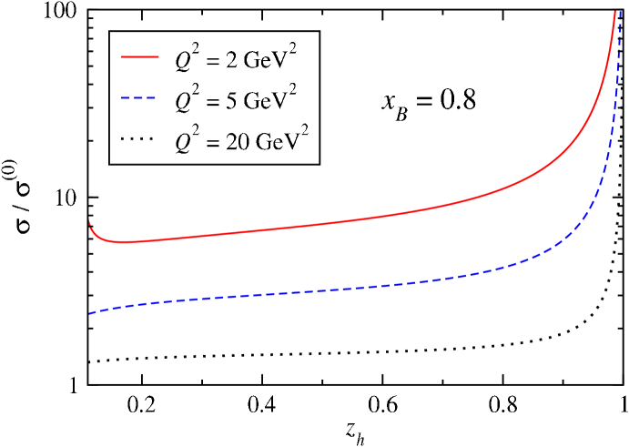
Figure 13: Ratio of cross sections $\sigma/\sigma^{(0)}$ for semi-inclusive charged-pion production (($\pi^{+}+\pi^{-})/2$) as a function of $z_{h}$ at several $Q^{2}$ values for $x_{B}=0.8$.

To illustrate most directly the effects of the HMCs, in Fig. 13 we consider charged pion production (average of $\pi^{+}$ and $\pi^{-}$) and plot as a function of $z_{h}$, for different $Q^{2}$ at $x_{B}=0.8$, the ratio of the full cross section $\sigma$ in Eq. (56) to the cross section $\sigma^{(0)}$, defined by taking the massless limit for the scaling variables $\sigma^{(0)}\equiv\sigma(\xi_{h}\to x_{B},\zeta_{h}\to z_{h})$ and setting $d\zeta_{h}/dz_{h}=1$. For the numerical computations we use the leading order CTEQ6L parton distributions [165] and the KKP leading order fragmentation functions [166], unless otherwise specified. The ratio at $x_{B}=0.8$ is strongly enhanced by nearly an order-of-magnitude at $Q^{2}=2$ GeV² for $z_{h}\lesssim 0.7$, but then becomes practically divergent in the limit $z_{h}\to 1$. This is of course an artifact of computing correction ratios with respect to “massless” cross sections that vanish at $z_{h}=1$ while the full cross section $\sigma$ remains finite due to rescaling by $(\xi_{h},\ \zeta_{h})$. The effect is naturally smaller at higher $Q^{2}$ values, but the rise at high $z_{h}$ is a common feature for all kinematics.

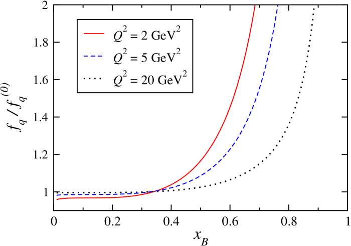
Figure 14: Ratio of the hadron mass corrected isoscalar parton distribution function $f_{q}(\xi_{h})$ for $q=u+d$ to the massless limit distribution $f_{q}^{(0)}$ as a function of $x_{B}$, for $m_{h}=m_{\pi}$ and $\zeta_{h}=0.2$.

On the other extreme of the spectrum, the small upturn in the ratios at low $z_{h}$ for the lowest $Q^{2}$ in Fig. 13 can be understood from the interplay between the finite-$Q^{2}$ kinematics and the shape of the fragmentation function. Assuming the fragmentation function is smooth, it is trivial to expand the ratio of corrected to uncorrected functions in a Taylor series as

$$\frac{D(\zeta_{h})}{D(z_{h})}\approx 1+\frac{D^{\prime}(z_{h})}{D(z_{h})}(\zeta_{h}-z_{h})\,.$$ (57)

The $z_{h}$ dependence of the HMCs arising in the fragmentation function is mostly determined by the negative shift in the fragmentation variable ($\zeta_{h}-z_{h}$) and by the local rate of change over $z_{h}$ of the fragmentation function. The pion fragmentation function generally behaves as a negative power of $z_{h}$ at small $z_{h}$, and the negative slope drives the ratio of corrected to uncorrected fragmentation functions upward as $z_{h}\to z_{h}^{\rm min}$, where $|\zeta_{h}-z_{h}|$ is maximum. For kaons and protons the slope of the form factor can be positive, which would suppress the mass corrected cross section in the vicinity of $z_{h}^{\rm min}$. In the limit $z_{h}\to 1$, on the other hand, the ratio $\sigma/\sigma^{(0)}$ becomes divergent for any kinematics and any hadron species because the cross section $\sigma^{(0)}\propto D(z_{h})$ vanishes, while the rescaled cross section remains finite.

At very small values of $z_{h}$ the factor $(1+m_{h}^{2}/\zeta_{h}Q^{2})$ in the definition of $\xi_{h}$ in Eq. (50) can render $\xi_{h}$ larger than $x_{B}$, suppressing the $\xi_{h}$-rescaled parton distributions relative to their asymptotic limit and driving $\sigma/\sigma^{(0)}$ slightly below unity. As discussed below, for heavier hadrons this effect will be more pronounced. The effect of the $\xi_{h}$ rescaling on the SIDIS cross section is illustrated explicitly in Fig. 14, where we show the ratio of the isoscalar parton distribution functions $f_{q}$, $q=u+d$, with [$f_{q}=f_{q}(\xi_{h})$] and without [$f_{q}^{(0)}=f_{q}(x_{B})$] hadron mass corrections, as a function of $x_{B}$ for $\zeta_{h}=0.2$ and $m_{h}=m_{\pi}$. At $Q^{2}=2$ GeV² the mass corrected parton distribution is several times larger than the uncorrected one at $x_{B}=0.8$, and even at $Q^{2}=20$ GeV² the HMC is some 50%, with the effect increasing dramatically as $x_{B}\to 1$. This sharp rise is analogous to that in inclusive DIS as seen in Fig. 3, and arises from $\xi_{h}$ being smaller than $x_{B}$ when the latter is large. In contrast, the $\xi_{h}$ rescaling effect becomes quite small at $x_{B}\lesssim 0.3$ for all the $Q^{2}$ considered, and in fact drives the ratio below unity, as discussed above.

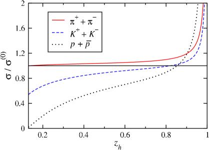
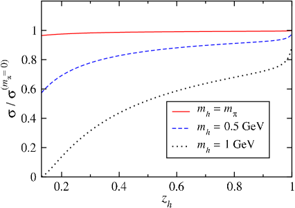
Figure 15: (Left) Dependence of the ratio of SIDIS cross sections $\sigma/\sigma^{(0)}$ with and without HMCs for different produced hadrons, $h=\pi^{+}+\pi^{-}$, $K^{+}+K^{-}$ or $p+\bar{p}$. (Right) Ratio of cross sections for $h=\pi^{+}+\pi^{-}$ for different values of the pion mass, relative to the massless cross section. In both cases the kinematics chosen are $x_{B}=0.3$ and $Q^{2}=5~{}$GeV².

The relative importance of HMCs for different produced hadron species is illustrated in the left panel of Fig. 15, where the ratio $\sigma/\sigma^{(0)}$ is shown as a function of $z_{h}$ for $x_{B}=0.3$ and $Q^{2}=5~{}$GeV². Over the range $0.3\lesssim z_{h}\lesssim 0.8$ the HMCs yield an upward correction of $\lesssim 10\%$ for the pions, but a downward correction of $\lesssim 20\%$ and $\lesssim 40\%$ for kaons and protons/antiprotons, respectively. At lower $z_{h}$ the cross section ratio for the heavier hadrons decreases dramatically because of the large suppression of the parton distribution from the $(1+m_{h}^{2}/\zeta_{h}Q^{2})$ factor in $\xi_{h}$, which overwhelms any other small-$z_{h}$ effect.

Note that in the left-hand side of Fig. 15 the appropriate fragmentation function for each produced hadron species has been used, which introduces a flavor dependence in the HMC because of the different fragmentation function shapes for each hadron. To isolate the effects of the hadron mass alone, on the RHS of Fig. 15 the ratios of cross sections computed with charged pion fragmentation functions and masses $m_{h}=m_{\pi}$ (= 0.139 GeV), 0.5 GeV and 1 GeV are shown relative to the cross section with $m_{\pi}=0$, for which $\zeta_{h}=z_{h}\xi/x_{B}$. One can see that in general increasing the hadron mass suppresses the cross section because of the $\xi_{h}$ scaling, and the inversion of the HMC hierarchy in the LHS of Fig. 15 going from low to high $z_{h}$ is due to the increasingly negative large-$z$ slope of the fragmentation functions for kaons and protons. While the differences at the physical pion mass are very small, for larger hadron masses $\sim 1$ GeV the effects can be quite significant at $z_{h}\lesssim 0.4$ even for $Q^{2}$ values of several GeV².

Experimental implications.

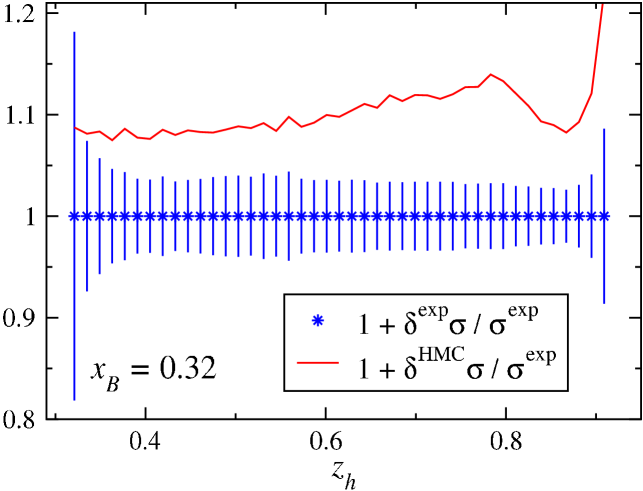
Figure 16: Comparison of the hadron mass correction to the SIDIS cross section for charged hadron production, $\delta^{\rm HMC}\sigma$, relative to the experimental cross section, $\delta^{\rm exp}\sigma$, with the relative experimental uncertainty as a function of $z_{h}$ for the Jefferson Lab experiment E00-108 [167] at $Q^{2}\sim 2.3$ GeV² and $x_{B}=0.32$.

The importance of the hadron mass corrections for experimental cross sections is examined in Fig. 16, where we compare the calculated difference $\delta^{\rm HMC}\sigma\equiv\sigma-\sigma^{(0)}$ with the experimental uncertainties $\delta^{\rm exp}\sigma$, normalized to the central values of the cross section for charged hadron production from Jefferson Lab [167]. As the JLab measurements are generally dominated by the semi-inclusive production of pions, $\xi_{h}\approx\xi$, and HMCs generally produce upward shifts relative to data. For the specific Jefferson Lab experiment E00-108 [167] of Fig. 16, $Q^{2}\sim 2.5$ GeV², with $x_{B}=0.32$, and the mass effects are approximately $2$ times larger than the experimental statistical errors. This illustrates the potentially significant impact that HMCs can have on leading-twist analyses of SIDIS data at moderate and large $x_{B}$ and low $Q^{2}$. To avoid these effects one would either need to go to smaller $x_{B}$ or larger $Q^{2}$ as might, for example, be afforded by the 12 GeV energy upgrade at Jefferson Lab. Alternatively, since the HMCs are calculated and model independent, lower $Q^{2}$ and higher $x_{B}$ data will still yield useful leading twist information provided the mass corrections are accounted for.

At higher energies, we find HMCs to fixed-angle measurements by the EMC [168] at large $x_{B}$ values to be negligible due to suppression by $Q^{2}$, which increases with $x_{B}$. Were these experiments conducted at smaller angles, however, it is likely that HMCs would become important.

Similarly, measurements at small $x_{B}\sim 0.001$ and $Q^{2}\gtrsim 12$ GeV² have been performed by the H1 collaboration [172] at HERA, and the data presented in terms of the fragmentation invariant $\eta_{h}$. The phenomenology of HMCs is markedly different in terms of $\eta_{h}$ from that discussed thus far in terms of $z_{h}$ because of the different functional forms for $\zeta_{h}$ in Eqs. (33), which constrains $\zeta_{h}>\eta_{h}$, and because of the Jacobian $d\zeta_{h}/d\eta_{h}$. In their analysis of the H1 data, Albino et al. [160] included the $\zeta_{h}$ rescaling of the fragmentation process, but neglected the effects of the target mass, which would be problematic for heavier hadrons such as kaons and protons. The H1 Collaboration measured charged hadron multiplicities, dominated by pions ($\sim$60%), with smaller contributions from kaons ($\sim$30%) and protons ($\sim$10%). In the measured $Q^{2}$ range the $m_{h}^{2}/Q^{2}$ term in $\xi_{h}$ is therefore strongly suppressed and at the typically low $x_{B}$ values one has $\xi\approx x_{B}$, so that overall we find the HMCs to be similar to those in Ref. [160]. However, for identified kaons, and especially protons, the SIDIS cross section would be more strongly suppressed compared to the results of Ref. [160] because $\xi_{h}\approx x_{B}(1+m_{h}^{2}/Q^{2})$ is significantly larger than $x_{B}$. This suppression may be non-negligible for the extraction of kaon and proton fragmentation functions from small-$x_{B}$ data. It therefore seems patent, particularly given the dramatic results of Fig. 16, that the nonperturbative mass of final state hadrons are a necessary analytical consideration in various processes; as always, this is especially true in the limit of small $Q^{2}$ and $x\sim 1$.

Chapter 4 Nonperturbative charm

“All the diversity, all the charm, and all the beauty of life are made up of light and shade.”
      — Leo Tolstoy

An improved grasp of the role played by heavy quarks is of critical importance for fully understanding the transition from the pQCD dynamics described in Chap. The nonperturbative structure of hadrons to the physics of color-neutral bound states. In particular, the constituent mass of the charm quark, $m_{c}\sim 1.3$ GeV, places the threshold for its production at the upper periphery of the nucleon excitation/resonance region discussed in some detail for elastic scattering in Chap. 1.2. Moreover, threshold effects in charm production are a necessary consideration for determinations of scaling violations and $Q^{2}$ dependence in QCD global analyses, as well as for computations of background processes in precision searches for novel physics outside the Standard Model.

Figure 1: At leading order, photon-gluon fusion predominates at $Q^{2}\sim m^{2}_{c}$ leading to the contribution to $F^{c}_{2}(x,Q^{2})$ given by Eq. (1).

In conventional analyses, charm is usually incorporated into the nucleon’s DIS structure functions by means of standard pQCD under the assumption that $c(x,Q^{2}\leq m^{2}_{c})=\bar{c}(x,Q^{2}\leq m^{2}_{c})\equiv 0$ below the physical charm production threshold $Q^{2}=m^{2}_{c}$. Any charm produced then for $Q^{2}>m^{2}_{c}$ enters extrinsically via perturbatively calculable diagrams, with the dominant leading order (LO) mechanisms coming from the gluon splitting and bremsstrahlung graphs depicted in Fig. 13, as well as from the boson-gluon fusion, or photon-gluon fusion process displayed in Fig. 1. For the former, we already saw in Chap.2.3 that generic DGLAP evolution stipulates convolutions of the charm distributions with pQCD splitting functions [Eq. (62)] according to Eq. (58). This procedure is numerically adequate at LO for large virtualities — i.e., $Q^{2}\gg m^{2}_{c}$, but at moderate kinematics characterized by $Q^{2}\sim m^{2}_{c}$, photon-gluon fusion is a more reliable approximation. Computing Fig. 1 by standard Feynman rules determined by Eq. (2), it can be shown that [173]

$$F^{c}_{2,\ {\rm PGF}}(x,Q^{2})\ =\ {\alpha_{s}(\mu^{2})\over 9\pi}\ \int_{x}^{z^{\prime}}\ {dz\over z}\ C^{\rm PGF}(z,Q^{2},m^{2}_{c})\cdot xg\left({x\over z},\mu^{2}\right)\ ,$$ (1a)

$$C^{\rm PGF}(z,Q^{2},m^{2}_{c})\ =\ 4\left\{1-2z+2z^{2}+4z(1-3z){m^{2}_{c}\over Q^{2}}-8z^{2}\left({m^{2}_{c}\over Q^{2}}\right)^{2}\right\}\ \ln\left({1+\beta\over 1-\beta}\right)$$

$$+\ \beta\left\{32z(1-z)-4-16z(1-z){m^{2}_{c}\over Q^{2}}\right\}\ ;\hskip 14.22636pt\beta\mathrel{\vbox{\hbox{\scriptsize.}\hbox{\scriptsize.}}}=\sqrt{1-{4z\over(1-z)}{m^{2}_{c}\over Q^{2}}}\ ;$$ (1b)

in Eq. (1a), to account for effects at the charm threshold, the upper bound on the convolution must be $z^{\prime}=1\Big{/}\Big{(}1+4m^{2}_{c}/Q^{2}\Big{)}$.

While this methodology and its extension to arbitrary order in perturbation theory are capable of predicting experimental results (especially at low $x$ and high $Q^{2}$) with admirable accuracy, potential nonperturbative effects may conspire to generate charm at more moderate $Q^{2}$ and higher $x$, signaling an intrinsic charm component of the nucleon. This would represent a fundamental contribution to the bound state structure of the nucleon apart from its known make-up consisting of a conventional mix of valence content with the light quark sea.

To estimate the plausibility and significance of this hypothesis, we first briefly review the existing literature concerning nonperturbative or intrinsic charm (IC) in the nucleon in Sec. 1. With this in mind, we then present in Secs. 2–3 the recently-published results of a comprehensive effective field theory calculation [175], which for the first time immediately connects intrinsic charm predictions to the $SU(4)$ hadronic spectrum. Finally, in Sec. 4 we constrain the model parameters of our formalism using the technology of a recently completed QCD global analysis [176].

1 Five-quark models of nucleon structure

In this section we review models of intrinsic charm based on particular five-quark Fock state components of the nucleon wave function. We will focus on models that describe the process by which a nucleon initially containing three light valence quarks transitions to a four quark plus one antiquark state containing a charm-anticharm quark pair as depicted in the final panel of Fig. 2.

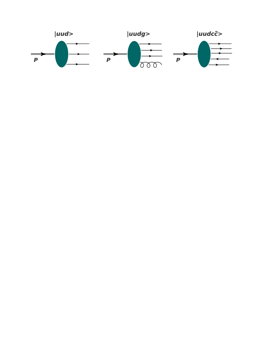
Figure 2: In the most basic conceptions, an intrinsic charm component appears in the higher states of a Fock space expansion of the proton wavefunction.

1 Scalar five-quark models

Before our calculation in [175], the various five-quark pictures essentially all involved the assumption of point-like interactions taken from naïve scalar field theories. Here we discuss some of the more archetypal options.

The BHPS model.

The earliest (and simplest) model for producing intrinsic charm was proposed over 30 years ago by Brodsky, Hoyer, Peterson, and Sakai (BHPS) [177]. In the infinite momentum frame (IMF) the probability for a proton with mass $M$ to make the transition $p\to uudc\bar{c}$ (or to a five-quark state containing any heavy quark pair) shown in the rightmost process of Fig. 2 involves an ‘old-fashioned’ perturbation theory energy denominator that can be rendered in terms of the masses $m_{i}$ and momentum fractions $x_{i}$ of its constituents,

$$P(p\to uudc\bar{c})\sim\left[M^{2}-\sum_{i=1}^{5}\frac{k_{\perp i}^{2}+m_{i}^{2}}{x_{i}}\right]^{-2}\ .$$ (2)

Here, $k_{\perp i}$ is the transverse momentum of quark $i$, and the heavy quarks in the $c\bar{c}$ pair are assigned indices $4$ and $5$.

For simplicity, the BHPS calculation assumed a point coupling for the $c\bar{c}$ production vertex, and neglected the effect of transverse momentum in the five-quark transition amplitudes. With the additional assumption that the charm mass is much greater than the nucleon and light quark masses, the probability for producing a single charm quark can be derived analytically,

$$P(x)=\frac{Nx^{2}}{2}\left[\frac{(1-x)}{3}\left(1+10x+x^{2}\right)+2x(1+x)\ln(x)\right]\ ,$$ (3)

with the normalization $N$ fixed by the overall charm quark probability in the proton. In Eq. (3), we have made the replacement $x_{5}\to x$ to go from Eq. (2).

Using the analytic expression (3) one obtains a “valence-like” (i.e., non-singular in the $x\rightarrow 0$ limit) charm quark distribution that is significant for $0.1\leq x\leq 0.5$. The valence-like shape arises from the structure of the energy denominator in Eq. (2), which for large quark masses $m_{i}$ favors configurations with large momentum fractions $x_{i}$. This feature is common to all similar five-quark models and invariably results in a valence-like heavy quark distribution.

It is also possible to compute the charm quark probability numerically without assuming that the charm quark mass is much greater than all other masses, though with realistic masses the charm quark distribution turns out to be similar to the analytic form of Eq. (3). Note also that since the charm and anticharm probabilities enter Eq. (2) symmetrically, the charm production mechanism in this model will produce equal probabilities for $c$ and $\bar{c}$, not unlike the pQCD contributions computed in, e.g., Eq. (1). Although the BHPS model is rather simplistic, it nevertheless provides a useful benchmark to test intrinsic charm and anticharm distributions obtained from other prescriptions.

The Pumplin model.

In a detailed study of intrinsic heavy quark probabilities, Pumplin [180] considered a series of models for the Fock space wave function on the light-front for a proton to make a transition to a four quark plus one antiquark system, with the heavy $q\bar{q}$ pair composed of either charm or bottom quarks. A simplified case was studied where a point scalar particle of mass $m_{0}$ couples with strength $g$ to $N$ scalar particles with masses $m_{1},m_{2},\ldots,m_{N}$. The light-front Fock space probability density $dP$ for such a process then takes the form [180]

$$dP = \frac{g^{2}}{(16\pi^{2})^{N-1}(N-2)!}\,\prod_{j=1}^{N}dx_{j}\,\delta\left(1-\sum_{j=1}^{N}x_{j}\right)\int_{s_{0}}^{\infty}ds\,\frac{(s-s_{0})^{N-2}}{(s-m_{0}^{2})^{2}}\,|F(s)|^{2}\ ,$$ (4)

where $s_{0}=\sum_{j=1}^{N}m_{j}^{2}/x_{j}$, and the form factor $F(s)$ serves to suppress contributions from high-mass states. If one neglects the effects of transverse momentum and the factors of $1/x_{j}$ in Eq. (4), and assumes a point form factor $F(s)=1$, then in the limit that the charm mass is much larger than all other masses one recovers the distribution in the BHPS model [177].

To incorporate the effects of the finite size of the nucleon, Pumplin considered both an exponential form factor,

$$|F(s)|^{2}=\exp\left[-(s-m_{0}^{2})/\Lambda^{2}\right]\ ,$$ (5)

and a power-law suppression factor,

$$|F(s)|^{2}={1\over(s+\Lambda^{2})^{n}}\ ,$$ (6)

with $\Lambda$ a cutoff mass regulator. Fixing the overall normalization to be a constant, the resulting shape of the charm quark momentum distribution with the power-law suppression, for a reasonable choice of $n=4$, turns out to be softer than the BHPS prediction for a range of cutoffs, $\Lambda=2-10$ GeV [180]. For the exponential suppression, the shape depends somewhat more strongly on the cutoff parameter, with the distribution being harder than the BHPS result for smaller $\Lambda$ values and softer for larger $\Lambda$. All of the resulting charm distributions are valence-like, however, with significant tails even beyond $x\approx 0.4$.

While these simple five-quark models give some qualitative insights into the possible generation of intrinsic charm at large $x$, they retain a high degree of dependence on the model parameters, whose connection with the underlying QCD dynamics is unclear. Furthermore, it is also not obvious how one could constrain the parameters phenomenologically by comparing deep-inelastic scattering with other observables, for instance. In the next section we discuss an alternative approach which may offer greater promise for relating intrinsic charm distributions to inputs determined from independent reactions.

2 Meson–baryon models

A hybrid class of intrinsic charm models that involves both quark and hadron degrees of freedom, and makes some unique and testable predictions for the $c$ and $\bar{c}$ distributions in the nucleon, are meson–baryon models (MBMs). Such models attempt to quantify the fluctuations of the nucleon to states with a virtual meson $M$ plus baryon $B$,

$$|N\rangle\ =\ \sqrt{Z_{2}}\,\left|N\right.\rangle_{0}\ +\ \sum_{M,B}\int\!dy\,d^{2}\bm{k}_{\perp}\,\phi_{MB}(y,k^{2}_{\perp})\,|M(y,\bm{k}_{\perp});B(1-y,-\bm{k}_{\perp})\rangle\ ,$$ (7)

where $\left|N\right.\rangle_{0}$ is the “bare”, three-quark nucleon state, and $Z_{2}$ is the wave function renormalization. The function $\phi_{MB}(y,k^{2}_{\perp})$ gives the probability amplitude for the physical nucleon to be in a state consisting of a virtual meson $M$ with longitudinal momentum fraction $y$ and transverse momentum $\bm{k}_{\perp}$, and a baryon $B$ with longitudinal momentum fraction $1-y$ and transverse momentum $-\bm{k}_{\perp}$. The total invariant mass squared of the meson–baryon system $s_{MB}$ can be written in the IMF as

$$s_{MB}(y,k^{2}_{\perp})=\frac{k^{2}_{\perp}+m_{M}^{2}}{y}+\frac{k^{2}_{\perp}+M_{B}^{2}}{1-y}\ ,$$ (8)

where $m_{M}$ and $M_{B}$ are the meson and baryon masses, respectively. If the meson–baryon terms include states containing charm quarks, the resulting probability distributions for anticharm and charm quarks in the nucleon can be written in the form of convolutions,

$$\bar{c}(x) = \sum_{M,B}\,\Big{[}\int_{x}^{1}\frac{dy}{y}\,f_{MB}(y)\,\bar{c}_{M}\Big{(}\frac{x}{y}\Big{)}+\int_{x}^{1}\frac{d\bar{y}}{\bar{y}}\,f_{BM}(\bar{y})\,\bar{c}_{B}\Big{(}\frac{x}{\bar{y}}\Big{)}\Big{]}\ ,$$ (9a)

$$c(x) = \sum_{B,M}\,\Big{[}\int_{x}^{1}\frac{d\bar{y}}{\bar{y}}\,f_{BM}(\bar{y})\,c_{B}\Big{(}\frac{x}{\bar{y}}\Big{)}+\int_{x}^{1}\frac{dy}{y}\,f_{MB}(y)\,c_{M}\Big{(}\frac{x}{y}\Big{)}\Big{]}\ ,$$ (9b)

where $\bar{y}\equiv 1-y$, and for ease of notation we have omitted the dependence of the distributions on the scale $Q^{2}$.

In analogy with the quark-gluon splitting functions of pQCD defined in Eq. (58), Eqs. (9) involve the splitting functions $f_{MB}(y)$ for a nucleon to fluctuate to meson $M$ with fraction $y$ of the proton’s momentum, and a spectator baryon $B$. The charm and anticharm distributions in the baryon $B$ are denoted by $c_{B}(z)$ and $\bar{c}_{B}(z)$, respectively, and carry a fraction $z=x/\bar{y}$ of the baryon’s momentum. On the same grounds, $f_{BM}(\bar{y})$ represents the splitting function for a nucleon fluctuating into a baryon $B$ with fraction $\bar{y}$ of the proton’s momentum, with a spectator meson $M$. The quark distributions inside the meson $M$ are denoted by $c_{M}(z)$ and $\bar{c}_{M}(z)$, respectively. If the charm quark resides exclusively in the baryon, with the anticharm in the meson (as is consistently the case in the present chapter), Eqs. (9) simplify further since

$$c_{M}(x)\ \to\ 0,\ \ \ \bar{c}_{B}(x)\ \to\ 0\ .$$ (10)

The splitting functions in Eqs. (9) are related to the probability amplitudes $\phi_{MB}$ by

$$f_{MB}(y) = \int_{0}^{\infty}d^{2}\bm{k}_{\perp}\,|\phi_{MB}(y,k^{2}_{\perp})|^{2}\ =\ f_{BM}(\bar{y})\ ,$$ (11)

where the reciprocity relation in the second equality arises from the conservation of $3$-momentum at the $MBN$ vertex [193, 194, 195]. This can be shown to be satisfied explicitly in the infinite momentum frame (or on the light-front), but is violated in covariant calculations [194, 195, 196] in the presence of $MBN$ form factors (or other ultraviolet regulators) which do not exhibit the $y\leftrightarrow\bar{y}$ symmetry of the amplitudes $\phi_{MB}$ [199].

The convolution equations (9) allow the symmetries of the splitting functions to be represented in terms of moments of the parton distributions $C^{(n)}$ and $\overline{C}^{(n)}$, defined as

$$\overline{C}^{(n)} = \int_{0}^{1}dx\,x^{n}\,\bar{c}(x)\ =\ \sum_{M,B}\,{\cal F}_{MB}^{(n)}\,\overline{C}_{M}^{(n)}\ ,$$ (12a)

$$C^{(n)} = \int_{0}^{1}dx\,x^{n}\,c(x)\ =\ \sum_{B,M}\,{\cal F}_{BM}^{(n)}\,C_{B}^{(n)}\ ,$$ (12b)

where

$${\cal F}_{MB}^{(n)} = \int_{0}^{1}dy\,y^{n}\,f_{MB}(y)\ ,$$ (13a)

$${\cal F}_{BM}^{(n)} = \int_{0}^{1}d\bar{y}\,\bar{y}^{n}\,f_{BM}(\bar{y})\ ,$$ (13b)

are the $n$-th moments of the splitting functions. The corresponding moments of the $\bar{c}$ and $c$ distributions in the meson $M$ and baryon $B$ are denoted $\overline{C}_{M}^{(n)}$ and $C_{B}^{(n)}$, respectively. In particular, the lowest moment of the splitting functions gives the average multiplicity of mesons $M$ and baryons $B$,

$$\langle n\rangle_{MB} \equiv {\cal F}_{MB}^{(0)}\ =\ {\cal F}_{BM}^{(0)}\ ,$$ (14)

which reflects global charge conservation, while conservation of momentum implies that the momentum fractions $\langle y\rangle_{MB}\equiv{\cal F}_{MB}^{(1)}$ and $\langle y\rangle_{BM}\equiv{\cal F}_{BM}^{(1)}$ are related by

$$\langle y\rangle_{BM}\ +\ \langle y\rangle_{MB} = \langle n\rangle_{MB}\ .$$ (15)

In contrast to the five-quark models discussed in Sec. 1, in which the $x$ dependence of the $c$ and $\bar{c}$ distributions was identical, in the MBM the distributions of heavy quarks and antiquarks in the nucleon are generally expected to be different. Indeed, since the $c$ in the baryon and $\bar{c}$ in the meson reside in rather different local environments, an asymmetry $c(x)\neq\bar{c}(x)$ is almost unavoidable. In fact, the experimental observation of $c(x)\neq\bar{c}(x)$, as might be extracted from charge asymmetries in charmed hadron production processes, is a trademark signal for nonperturbative charm [197]. Of course, since the proton has no net charm, the lowest moments of $c$ and $\bar{c}$ must cancel; however, all higher moments will be nonzero,

$$C^{(0)}-\overline{C}^{(0)}=0\ ,\ \ \ \ \ \ \ C^{(n)}-\overline{C}^{(n)}\neq 0\ \ (n\geq 1)\ ,$$ (16)

with the result of Eq. (55) ensuring the first relation for all $Q^{2}$ — up to NLO corrections. In general, however, the realization of Eq. (14) guarantees the proton to have no net charm at the nonperturbative scale $Q^{2}=m^{2}_{c}$.

Because quarks and antiquarks possess opposite intrinsic parities, parity conservation will require that the quark wave functions respect overall parity conservation. For example, if the initial proton state is treated as three constituent $(uud)$ quarks in $S$-wave orbitals and a $c\bar{c}$ pair is added, then the placement of a charm quark in an $S$ state necessitates that anticharm be in an odd-parity configuration. In the MBM, this behavior is accommodated by proper use of physical vertices that correctly account for the spin degrees of freedom of the relevant fields. As a rule, models that treat quarks as scalar point-like particles, for example, will therefore not satisfy these constraints [180, 181].

Table 1: Lowest mass meson–baryon Fock states of the proton containing charm and anticharm quarks. For each state the isospin $I$, spin $J$ and parity $P$ are listed for the meson and baryon, together with the masses.

Baryon	$I(J^{P})$	Meson	$I(J^{P})$
$p\,(938)$	$\frac{1}{2}\,(\frac{1}{2}^{+})$	$J/\psi(3097)$	$0\,(1^{-})$
$\Lambda_{c}^{+}(2286)$	$0\,(\frac{1}{2}^{+})$	$\bar{D}^{0}(1865)$	$\frac{1}{2}\,(0^{-})$
		$\bar{D}^{*0}(2007)$	$\frac{1}{2}\,(1^{-})$
$\Sigma_{c}^{+}(2455)$	$1\,(\frac{1}{2}^{+})$	$\bar{D}^{0}(1865)$	$\frac{1}{2}\,(0^{-})$
		$\bar{D}^{*0}(2007)$	$\frac{1}{2}\,(1^{-})$
$\Sigma_{c}^{++}(2455)$	$1\,(\frac{1}{2}^{+})$	$D^{-}(1870)$	$\frac{1}{2}\,(0^{-})$
		$D^{*-}(2010)$	$\frac{1}{2}\,(1^{-})$
$\Sigma_{c}^{*+}(2520)$	$1\,(\frac{3}{2}^{+})$	$\bar{D}^{0}(1865)$	$\frac{1}{2}\,(0^{-})$
		$\bar{D}^{*0}(2007)$	$\frac{1}{2}\,(1^{-})$
$\Sigma_{c}^{*++}(2520)$	$1\,(\frac{3}{2}^{+})$	$D^{-}(1870)$	$\frac{1}{2}\,(0^{-})$
		$D^{*-}(2010)$	$\frac{1}{2}\,(1^{-})$

In the present analysis, we consider various meson–baryon states containing charm quarks that could contribute to the intrinsic charm in the proton, as summarized in Table 1. These include the SU(4) octet isoscalar $\Lambda_{c}$ and isovector $\Sigma_{c}$ baryons, and the decuplet $\Sigma_{c}^{*}$, while for the mesons, the pseudoscalar $D$ and vector $D^{*}$ mesons are included. In addition, the state involving a proton fluctuation to $p+J/\psi$, where both the $c$ and $\bar{c}$ reside in the $J/\psi$, was considered in Ref. [180]. Although this has a combined mass which is actually lower than all the other charmed meson–baryon configurations, its contribution should be strongly suppressed by the OZI rule.

To constrain the model parameters in the calculations — namely, the hadronic couplings and form factor cutoffs — we use phenomenological input from $DN$ and $\bar{D}N$ scattering analyses [186, 187, 188, 189], together with inclusive charmed baryon production data in $pp$ collisions. We discuss the formal aspects of these considerations in Sec. 1 after first deriving in the next section the splitting functions $f_{MB}(y)$ for the various configurations in Table 1, as well as the associated distributions $c_{B}(z),\bar{c}_{M}(z)$ within them.

2 Amplitudes for IC

Derivation of meson–baryon splitting functions.

The essential ingredients of the two-step meson-baryon models are amplitudes formulated separately at hadron- and quark-level, which then undergo convolution per Eq. (9). Here we outline the technical details of the derivations of the splitting functions for the dissociation of a nucleon with $4$-momentum $P$ into a meson $M$ with momentum $k$ and baryon $B$ with momentum $p$. We consider dissociations into the SU(4) octet isoscalar $\Lambda_{c}$ and isovector $\Sigma_{c}$ baryons, and the decuplet $\Sigma_{c}^{*}$ baryon, accompanied by the charmed pseudoscalar $D$ and vector $D^{*}$ mesons. The transitions to specific isospin states are obtained using appropriate isospin transition factors, as discussed in Sec. 1.

The contribution of a specific meson–baryon component to the nucleon hadronic tensor $W_{\mu\nu}^{N}$ is defined in terms of the contributions $\delta^{[MB]}F_{1,2}^{N}$ to the structure functions as [22]

$$\delta^{[MB]}W_{\mu\nu}^{N}(P,q) = \widetilde{g}_{\mu\nu}\,\delta^{[MB]}F_{1}^{N}\ +\ \frac{\widetilde{P}_{\mu}\widetilde{P}_{\nu}}{P\cdot q}\,\delta^{[MB]}F_{2}^{N}\ ,$$ (17)

where $q$ is the $4$-momentum of the external electromagnetic field.

For reasons that will become clear in the subsequent discussion, we find it advantageous to compute strictly forward-propagating diagrams in the IMF. Within the framework of time-ordered perturbation theory evaluated in IMF kinematics ($P_{L}\to\infty$), with intermediate state particles on their mass-shells but off their “energy-shells”, the standard decomposition for the momentum variables is [209]

$$P_{0} = P_{L}+\frac{M^{2}}{2P_{L}}+{\cal O}\left(\frac{1}{P_{L}^{2}}\right)\ ,$$ (18a)

$$k_{0} = |y|P_{L}+\frac{k^{2}_{\perp}+m_{M}^{2}}{2|y|P_{L}}+{\cal O}\left(\frac{1}{P_{L}^{2}}\right)\ ,$$ (18b)

$$p_{0} = |1-y|P_{L}+\frac{k^{2}_{\perp}+M_{B}^{2}}{2|1-y|P_{L}}+{\cal O}\left(\frac{1}{P_{L}^{2}}\right)\ ,$$ (18c)

for the energies, and

$$\bm{k} = |y|\bm{P}+\bm{k_{\perp}}\ ,$$ (19a)

$$\bm{p} = |1-y|\bm{P}-\bm{k_{\perp}}\ ,$$ (19b)

for the $3$-momenta, with $\bm{k}_{\perp}\cdot\bm{P}=0$. In the non-vanishing forward limit one has $y\in[0,1]$, such that $|1-y|=(1-y)$.

Obeying the standard rules [190] for computing forward-moving TOPT diagrams such as Fig. 3, we find on purely general grounds

$$\delta^{[MB]}W_{\mu\nu}^{N}\ =\ \int{d^{3}{\bf k}\over(2\pi)^{3}(2P_{0})(2k_{0})^{2}}\,\frac{g^{2}_{MBN}({\bf k})}{(P_{0}-p_{0}-k_{0})^{2}}N^{MB}_{\mu\nu}\ ;$$ (20)

it is straightforward to show that the perturbation theory energy denominator can be rewritten as $(P_{0}-p_{0}-k_{0})=(M^{2}-s_{MB})\Large/2P_{L}$, where the center-of-mass energy $s_{MB}$ is as defined in Eq. (8). It is in fact simpler to translate to the space spanned by the parameters $(y,k^{2}_{\perp})$; keeping track of the phase space factor $d^{3}{\bf k}\rightarrow dydk^{2}_{\perp}$, and using the kinematical definitions of Eq. (18), we find that the generic one-loop diagram for the scattering from the meson $M$ evaluates to

$$\delta^{[MB]}W_{\mu\nu}^{N} = \frac{g^{2}_{DBN}}{16\pi^{2}}\int_{0}^{1}dy\int_{0}^{\infty}\frac{dk^{2}_{\perp}}{y(1-y)}\frac{|F(s)|^{2}}{(M^{2}-s)^{2}}\ N^{MB}_{\mu\nu}\ ,$$ (21)

where $y$ is the longitudinal momentum fraction carried by the meson, $F(s)$ is the $MBN$ hadronic factor, with the invariant mass squared of the $MB$ system $s$ defined in Eq. (8). The tensor $N^{MB}_{\mu\nu}$ is computed from the spin trace of the appropriate meson and baryon propagators and vertices, with explicit forms given below.

In addition, we shall find that the expression in Eq. (21) is generally evaluated in terms of inner products $P\cdot k$, $P\cdot p$ and $P\cdot k$ computed from Eqs. (18) and (19) as

$$P\cdot k =\ {1\over 2y}\ \Big{(}k^{2}_{\perp}+m^{2}_{M}+y^{2}M^{2}\Big{)}\ ,$$ (22a)

$$P\cdot p =\ {1\over 2(1-y)}\ \Big{(}k^{1}_{\perp}+M^{2}_{B}+(1-y)^{2}M^{2}\Big{)}\ ,$$ (22b)

$$p\cdot k =\ k^{2}_{\perp}\ +\ {y(k^{2}_{\perp}+M^{2}_{B})\over 2(1-y)}\ +\ {(1-y)\cdot(k^{2}_{\perp}+m^{2}_{M})\over 2y}\ ;$$ (22c)

the corrections to the structure functions $\delta^{[MB]}F_{1,2}^{N}$ follow after equating the coefficients of the tensors in Eqs. (17) and (21). The corrections to the $c$ and $\bar{c}$ distributions in Eqs. (9) may then be extracted from $\delta^{[MB]}F_{1,2}^{N}$ using parton model relations analogous to Eq. (31) as we now demonstrate.

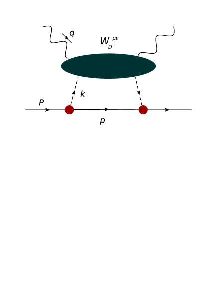
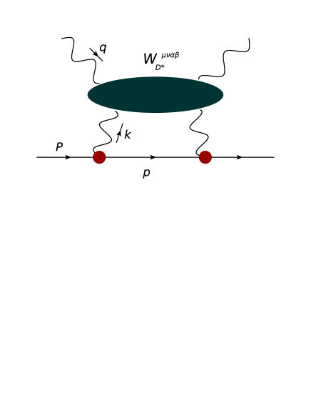
Figure 3: Diagrams for the $p\rightarrow DB$ (left) and $p\rightarrow D^{*}B$ (right) processes.

$N\to DB$ splitting

The dissociation of a nucleon to a spin-1/2 charmed baryon $B=\Lambda_{c}$ or $\Sigma_{c}$ and a pseudoscalar $D$ meson is derived from the effective hadronic lagrangian [189]

$${\cal L}_{DBN} = ig\,\bar{\psi}_{N}\,\gamma_{5}\,\psi_{B}\,\phi_{D}\ +\ \mathrm{h.c.}\ ,$$ (23)

where $\psi_{N}$ and $\psi_{B}$ are the nucleon and charmed baryon fields, respectively, $\phi_{D}$ is the spin-0 $D$ meson field, and the coupling constant $g\to g_{DBN}$. Treating the propagation of the meson and baryon fields as appropriate for point particles, the trace factor $N^{DB}_{\mu\nu}$ can be written as

$$N_{\mu\nu}^{DB} = \frac{1}{2}\ \sum_{s,s^{\prime}}\ \mathrm{Tr}\left[\bar{u}^{N}_{s}(P)(i\gamma_{5})u^{B}_{s^{\prime}}(p)\,W^{D}_{\mu\nu}(k,q)\,\bar{u}^{B}_{s^{\prime}}(p)(i\gamma_{5})u^{N}_{s}(P)\right]$$ (24)

$$= \frac{1}{2}\mathrm{Tr}\left[i\gamma_{5}(\not{P}+M)i\gamma_{5}\,W^{D}_{\mu\nu}(k,q)\,(\not{p}+M_{B})\right]$$

$$= -\frac{1}{2}\mathrm{Tr}\left[(\gamma_{5})^{2}(-\not{P}+M)\,(\not{p}+M_{B})\right]\,\widetilde{g}_{\mu\nu}F_{1}^{D}\,+\,\dots$$

$$= \left(2P\cdot p-2MM_{B}\right)\,\widetilde{g}_{\mu\nu}F_{1}^{D}\,+\,\dots\ ,$$

where $W_{D}^{\mu\nu}$ is the hadronic tensor for the $D$ meson, with a form similar to that in Eq. (17), and $F_{1}^{D}$ is the corresponding structure function which depends on the $\bar{c}$ distribution in $D$. Note also that to reduce the first line of Eq. (24) we used the property of the nucleon/baryon spinors that

$$\sum_{s}u_{s}(P)\cdot\bar{u}_{s}(P)\ =\ (\not{P}+M)\ {u\bar{u}\over 2M}\ ,\hskip 14.22636ptu\bar{u}\equiv 2M\$$ (25)

— a step we shall perform implicitly in the subsequent computations of this section. Using Eq. (22), and equating the coefficients of $\widetilde{g}_{\mu\nu}$ in Eqs. (17), (21) and (24) then yields the convolution expression in Eq. (9a) in which we identify the hadronic splitting function as

$$f_{DB}(y) = T_{B}\frac{g^{2}}{16\pi^{2}}\int{dk_{\perp}^{2}\over y(1-y)}{|F(s)|^{2}\over(s-M^{2})^{2}}\left[\frac{k_{\perp}^{2}+(M_{B}-(1-y)M)^{2}}{1-y}\right]\ ,$$ (26)

where for ease of notation we have used for the coupling constant $g\to g_{DBN}$ and for the $DB$ invariant mass $s\to s_{DB}$. The isospin transition factor $T_{B}$ is given by

$$T_{B}=1+\delta_{t_{B},+1}\ ,$$ (27)

in which the third component of the isospin of the charmed baryon is $t_{B}=0$ for $B=\Lambda_{c}^{+}$ and $\Sigma_{c}^{+}$, and $t_{B}=+1$ for $B=\Sigma_{c}^{++}$. The states described by the splitting function $f_{DB}(y)$ include the lowest-mass configuration $\bar{D}^{0}\Lambda_{c}^{+}$, as well as the isovector charmed baryon states $\bar{D}^{0}\Sigma_{c}^{+}$ and $D^{-}\Sigma_{c}^{++}$.

Performing an analogous calculation for the recoil process involving scattering from the baryon $B$ confirms the symmetry relation (11), which follows from the global charge and momentum conservation relations in Eqs. (14) and (15). Specifically, we evaluate the recoil analogue of the left diagram in Fig. 3, with scattering from an interacting baryon of $4$-momentum $p$. Much as before, the trace algebra yields

$$N_{\mu\nu}^{BD} = \frac{1}{2}\mathrm{Tr}\left[i\gamma_{5}(\not{P}+M)i\gamma_{5}\,W^{B}_{\mu\nu}(k,q)\,(\not{p}+M_{B})\right]$$ (28)

$$= \left(2P\cdot p-2MM_{B}\right)\,\widetilde{g}_{\mu\nu}F_{1}^{B}\,+\,\dots\ ,$$

though we must evaluate this using the proper recoil kinematics. These are now

$$P_{0} = P_{L}+\frac{M^{2}}{2P_{L}}+{\cal O}\left(\frac{1}{P_{L}^{2}}\right)\ ,$$ (29a)

$$p_{0} = |\bar{y}|P_{L}+\frac{k^{2}_{\perp}+M_{B}^{2}}{2|\bar{y}|P_{L}}+{\cal O}\left(\frac{1}{P_{L}^{2}}\right)\ ,$$ (29b)

$$k_{0} = |1-\bar{y}|P_{L}+\frac{k^{2}_{\perp}+m_{M}^{2}}{2|1-\bar{y}|P_{L}}+{\cal O}\left(\frac{1}{P_{L}^{2}}\right)\ ,$$ (29c)

for the $0$-components, while for the $3$-momenta we require

$$\bm{p} = |\bar{y}|\bm{P}+\bm{k_{\perp}}\ ,$$ (30a)

$$\bm{k} = |1-\bar{y}|\bm{P}-\bm{k_{\perp}}\ ,$$ (30b)

with $\bm{k}_{\perp}\cdot\bm{P}=0$ as before, and an appropriate redefinition of the baryon-meson invariant mass must be made vis-á-vis Eq. (8): $s_{MB}(y,k^{2}_{\perp})\rightarrow\bar{s}_{BM}(\bar{y},k^{2}_{\perp})$. Performing a series of deductions with these definitions similar to those used to obtain Eq. (26) leads to

$$f_{BD}(\bar{y}) = T_{B}\frac{g^{2}}{16\pi^{2}}\int{dk_{\perp}^{2}\over\bar{y}(1-\bar{y})}{|F(\bar{s})|^{2}\over(\bar{s}-M^{2})^{2}}\left[\frac{k_{\perp}^{2}+(M_{B}-\bar{y}M)^{2}}{\bar{y}}\right]\ ,$$ (31)

in which the reciprocity of Eq. (11) is clearly manifest. Similar operations with the following amplitudes also confirm such symmetry relations in each case.

$N\to D^{*}B$ splitting

For the interaction between the nucleon and spin-1/2 baryon with a vector $D^{*}$ meson, the effective lagrangian is given by [189]

$${\cal L}_{D^{*}BN} = g\,\bar{\psi}_{N}\gamma_{\mu}\,\psi_{B}\,\theta_{D^{*}}^{\mu}\ +\ \frac{f}{4M}\bar{\psi}_{N}\sigma_{\mu\nu}\psi_{B}\,F_{D^{*}}^{\mu\nu}\ +\ \mathrm{h.c.}\ ,$$ (32)

where $\theta_{D^{*}}^{\mu}$ is the vector meson field, with field strength tensor $F_{D^{*}}^{\mu\nu}=\partial^{\mu}\theta_{D^{*}}^{\nu}-\partial^{\nu}\theta_{D^{*}}^{\mu}$, the tensor operator $\sigma_{\mu\nu}=(i/2)[\gamma_{\mu},\gamma_{\nu}]$, and the vector and tensor couplings are $g\to g_{D^{*}BN}$ and $f\to f_{D^{*}BN}$. In this case the trace factor $N_{\mu\nu}^{D^{*}B}$ is given by

$$N_{\mu\nu}^{D^{*}B} = \frac{1}{2}\mathrm{Tr}\bigg{[}(\not{P}+M)\Big{(}g\gamma^{\alpha}+\frac{f}{2M}(\Delta^{\alpha}-\gamma^{\alpha}\not{\Delta})\Big{)}(\not{p}+M_{B})$$ (33)

$$\hskip 62.59596pt\times\Big{(}g\gamma^{\beta}-\frac{f}{2M}(\Delta^{\beta}-\gamma^{\beta}\not{\Delta})\Big{)}\bigg{]}\,W^{D^{*}}_{\mu\nu\alpha\beta}(k,q)$$

$$= \bigg{(}g^{2}G_{v}+\frac{gf}{M}G_{vt}+\frac{f^{2}}{M^{2}}G_{t}\bigg{)}\,\widetilde{g}_{\mu\nu}F_{1}^{D^{*}}\ +\ \dots\ ,$$

where $\Delta=P-p$, and the kinematical factors $G_{v}$, $G_{vt}$ and $G_{t}$ are given below in Eqs. (36). The rank-4 tensor for the interacting $D^{*}$ meson can be expressed in the form [194]

$$W^{D^{*}}_{\mu\nu\alpha\beta}(k,q) = \Big{(}\widetilde{g}_{\mu\nu}F_{1}^{D^{*}}+\frac{\widetilde{k}_{\mu}\widetilde{k}_{\nu}}{m^{2}_{D^{*}}}F_{2}^{D^{*}}\Big{)}\,\widetilde{g}_{\alpha\beta}\ ,$$ (34)

with $F_{1,2}^{D^{*}}$ the corresponding vector meson structure functions.

Thus for the dissociation of the proton to a charmed vector meson $D^{*}=\bar{D}^{*0}$ or $D^{*-}$ and spin-1/2 charmed baryon, the corresponding splitting function is given by a sum of vector ($G_{v}$), tensor ($G_{t}$) and vector-tensor interference ($G_{vt}$) terms,

$$f_{D^{*}B}(y) = T_{B}\frac{1}{16\pi^{2}}\int{dk_{\perp}^{2}\over y(1-y)}{|F(s)|^{2}\over(s-M^{2})^{2}}$$ (35)

$$\times\left[g^{2}\,G_{v}(y,k_{\perp}^{2})\ +\ {gf\over M}\,G_{vt}(y,k^{2}_{\perp})\ +\ \frac{f^{2}}{M^{2}}\,G_{t}(y,k^{2}_{\perp})\right]\ ,$$

where

$$G_{v}(y,k_{\perp}) = {1\over 2}\mathrm{Tr}\Big{[}(\not{P}+M)\gamma^{\alpha}(\not{p}+M_{B})\gamma^{\beta}\Big{]}\,\tilde{g}_{\alpha\beta}$$ (36a)

$$= -6MM_{B}\ +\ \frac{4(P\cdot k)(p\cdot k)}{m_{D}^{2}}\ +\ 2P\cdot p\ ,$$

$$G_{vt}(y,k_{\perp}) = {1\over 4}\mathrm{Tr}\Big{[}(\not{P}+M)(\Delta^{\alpha}-\gamma^{\alpha}\not{\Delta})(\not{p}+M_{B})\gamma^{\beta}$$ (36b)

$$\hskip 42.67912pt-\ (\not{P}+M)\gamma^{\alpha}(\not{p}+M_{B})(\Delta^{\beta}-\gamma^{\beta}\not{\Delta})\Big{]}\,\tilde{g}_{\alpha\beta}$$

$$= 4(M+M_{B})(P\cdot p-MM_{B})$$

$$-\ \frac{2}{m_{D}^{2}}\left[M_{B}(P\cdot k)^{2}-(M+M_{B})(P\cdot k)(p\cdot k)+M(p\cdot k)^{2}\right]\ ,$$

$$G_{t}(y,k_{\perp}) = {1\over 8}\mathrm{Tr}\Big{[}(\not{P}+M)(\Delta^{\alpha}-\gamma^{\alpha}\not{\Delta})(\not{p}+M_{B})(\gamma^{\beta}\not{\Delta}-\Delta^{\beta})\Big{]}\,\tilde{g}_{\alpha\beta}$$ (36c)

$$= -(P\cdot p)^{2}\ +\ (M+M_{B})^{2}\,P\cdot p\ -\ MM_{B}(M^{2}+M_{B}^{2}+MM_{B})$$

$$+\ \frac{1}{2m_{D}^{2}}\Big{[}(P\cdot p-MM_{B})[(P-p)\cdot k]^{2}-2(M_{B}^{2}P\cdot k-M^{2}p\cdot k)[(P-p)\cdot k]$$

$$\hskip 28.45274pt+2(P\cdot k)(p\cdot k)(2P\cdot k-M_{B}^{2}-M^{2})\Big{]}\ ,$$

and where $p$ is the $4$-momentum of the baryon, and the inner products $P\cdot p$, $P\cdot k$ and $p\cdot k$ have again been computed explicitly in Eq. (22). The splitting function $f_{D^{*}B}(y)$ describes transitions to the states $\bar{D}^{*0}\Lambda_{c}^{+}$, $\bar{D}^{*0}\Sigma_{c}^{+}$ and $D^{*-}\Sigma_{c}^{++}$, and the isospin transition factor $T_{B}$ is as in Eq. (27). As before, for compactness we have again used the shorthand notation for the couplings $g\to g_{D^{*}BN}$ and $f\to f_{D^{*}BN}$, with $s\to s_{D^{*}B}$.

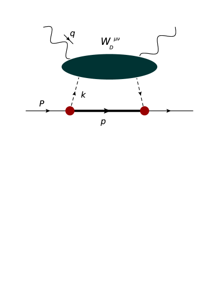
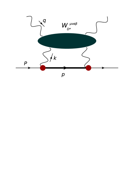
Figure 4: Diagrams for the $p\rightarrow DB^{*}$ (left) and $p\rightarrow D^{*}B^{*}$ (right) processes.

$N\to DB^{*}$ splitting

The interaction of a nucleon with a spin-3/2 charmed baryon $B^{*}=\Sigma_{c}^{*}$ and a pseudoscalar meson can be calculated using the lagrangian [189]

$${\cal L}_{DB^{*}N} = \frac{f}{m_{D}}\Big{(}\bar{\Psi}_{B^{*}}^{\mu}\,\psi_{N}\,\partial_{\mu}\phi_{D}\ +\ \bar{\psi}_{N}\Psi_{B^{*}}^{\mu}\partial_{\mu}\phi_{D}\Big{)}\ ,$$ (37)

where $\Psi_{B^{*}}^{\mu}$ is the Rarita-Schwinger spinor-vector field, and the coupling $f\to f_{DB^{*}N}$. From Eq. (37) and the LHS diagram of Fig. 4, the trace factor tensor is

$$N_{\mu\nu}^{DB^{*}} = \frac{1}{2}\mathrm{Tr}\bigg{[}(\not{P}+M)\,\Lambda^{\alpha\beta}_{B^{*}}(p)\,\Delta_{\alpha}\Delta_{\beta}\,W_{\mu\nu}^{D}(k,q)\bigg{]}$$ (38)

$$= \frac{4}{3}\left(P\cdot p+MM_{B^{*}}\right)\left(\frac{(p\cdot\Delta)^{2}}{M_{B^{*}}^{2}}-\Delta^{2}\right)\widetilde{g}^{\mu\nu}\,F_{1}^{D}\ +\ \dots\ ,$$

where the energy projector for the spinor-vector is

$$\Lambda^{\alpha\beta}_{B^{*}}(p) = (\not{p}+M_{B^{*}})\left(-g^{\alpha\beta}+{\gamma^{\alpha}\gamma^{\beta}\over 3}+{\gamma^{\alpha}p^{\beta}-\gamma^{\beta}p^{\alpha}\over 3M_{B^{*}}}+{2\,p^{\alpha}p^{\beta}\over 3M_{B^{*}}^{2}}\right)\ .$$ (39)

The inner products in Eq. (38) can once again be worked out in terms of $y,k^{2}_{\perp}$ using the definitions in Eq. (22) with the replacement $B\to B^{*}$, which leads directly to the desired hadronic amplitude for fluctuations to spin-3/2 charmed baryons $B^{*}=\Sigma_{c}^{*+}$ and $\Sigma_{c}^{*++}$. Namely, for the dissociations of a proton to states with a spin-0 $D$ meson, $\bar{D}^{0}\Sigma_{c}^{*+}$ and $D^{-}\Sigma_{c}^{*++}$, the splitting function is given by

$$f_{DB^{*}}(y) = T_{B^{*}}\frac{g^{2}}{16\pi^{2}}\int{dk_{\perp}^{2}\over y(1-y)}{|F(s)|^{2}\over(s-M^{2})^{2}}$$ (40)

$$\times{\left[k_{\perp}^{2}+(M_{B^{*}}-(1-y)M)^{2}\right]\left[k_{\perp}^{2}+(M_{B^{*}}+(1-y)M)^{2}\right]^{2}\over 6M_{B^{*}}^{2}(1-y)^{3}}\ ,$$

with $g\to g_{DB^{*}N}$ and $s\to s_{DB^{*}}$. The isospin transition factor $T_{B^{*}}$ here is similar to that in Eq. (27), but with the third component of the charmed baryon isospin $t_{B^{*}}=0$ for $B^{*}=\Sigma_{c}^{*+}$ and $t_{B^{*}}=+1$ for $B^{*}=\Sigma_{c}^{*++}$.

$N\to D^{*}B^{*}$ splitting

Finally, for the nucleon splitting to a spin-3/2 charmed baryon $B^{*}$ coupled to a vector meson $D^{*}$ the effective hadronic lagrangian is given by [189]

$${\cal L}_{D^{*}B^{*}N} = \frac{f}{m_{D^{*}}}i\Big{(}\bar{\Psi}_{B^{*}\nu}\gamma^{5}\gamma_{\mu}\psi_{N}-\bar{\psi}_{N}\gamma^{5}\gamma_{\mu}\Psi_{B^{*}\nu}\Big{)}F_{D^{*}}^{\mu\nu}\ ,$$ (41)

where $f\to f_{D^{*}B^{*}N}$. This yields the resulting trace tensor

$$N_{\mu\nu}^{D^{*}B^{*}} = \frac{1}{2}\mathrm{Tr}\bigg{[}(\not{P}+M)\gamma^{5}\gamma^{\alpha}\,\Lambda_{B^{*}}^{\alpha^{\prime}\beta^{\prime}}(p)\,\gamma^{5}\gamma^{\beta}\bigg{]}\mathcal{G}_{\alpha\beta\alpha^{\prime}\beta^{\prime}}\,\widetilde{g}_{\mu\nu}F_{1}^{D^{*}}\ +\ \dots\ ,$$ (42)

for which we define

$$\mathcal{G}_{\alpha\beta\alpha^{\prime}\beta^{\prime}} = \Delta_{\alpha\beta}\,\widetilde{g}_{\alpha^{\prime}\beta^{\prime}}-\Delta_{\alpha\beta^{\prime}}\,\widetilde{g}_{\alpha^{\prime}\beta}-\Delta_{\alpha^{\prime}\beta}\,\widetilde{g}_{\alpha\beta^{\prime}}+\Delta_{\alpha^{\prime}\beta^{\prime}}\,\widetilde{g}_{\alpha\beta}\ ,$$ (43)

with $\Delta_{\alpha\beta}\equiv\Delta_{\alpha}\Delta_{\beta}$, the other expressions having been defined above. Evaluating the trace in Eq. (42) and equating coefficients of the $\widetilde{g}_{\mu\nu}$ terms then leads to the convolution relation with the splitting function for the fluctuations to states with $D^{*}$ mesons and spin-3/2 baryons $B^{*}$ given by

$$f_{D^{*}B^{*}}(y) = T_{B^{*}}\frac{g^{2}}{m_{D^{*}}^{2}16\pi^{2}}\int{dk_{\perp}^{2}\over y(1-y)}{|F(s)|^{2}\over(s-M^{2})^{2}}$$

$$-\ \left[\frac{4MM_{B^{*}}}{3}\Big{(}2M_{B^{*}}^{2}+MM_{B^{*}}+2M^{2}\Big{)}-\frac{4MM_{B^{*}}}{3m_{D^{*}}^{2}}((P-p)\cdot k)^{2}\right.$$

$$-\ \frac{4}{3m_{D^{*}}^{2}}\Big{(}M_{B^{*}}^{2}(P\cdot k)^{2}+M^{2}(p\cdot k)^{2}\Big{)}+\frac{4P\cdot p}{3}\Big{(}2M_{B^{*}}^{2}+4MM_{B^{*}}+M^{2}\Big{)}$$

$$\left.+\ \frac{4P\cdot p}{3m_{D^{*}}^{2}}(p\cdot k)^{2}\Big{(}1-\frac{M^{2}}{M_{B^{*}}^{2}}\Big{)}-4(P\cdot p)^{2}\left(1-\frac{2(P\cdot k)(p\cdot k)}{3m_{D^{*}}^{2}M_{B^{*}}^{2}}-\frac{P\cdot p}{3M_{B^{*}}^{2}}\right)\right]\ ,$$

where $g\to g_{D^{*}B^{*}N}$, $s\to s_{D^{*}B^{*}}$, and the inner products in Eq. (2) are given by Eq. (22) after the replacements $D\to D^{*}$ and $B_{c}\to\Sigma_{c}^{*}$.

Charm content of charmed baryons and mesons.

In the literature estimates of the distributions of heavy quarks in heavy hadrons have been made using the heavy quark limit [178], and within a scalar constituent quark model [180]. Collecting and building upon several features of these approaches in constructing a relativistic quark model with the correct spin degrees of freedom, we compute results analogous to the hadronic splittings derived above. Again we apply the time-ordered perturbation theory framework in the IMF, but now at parton-level, defining the IMF momentum fraction $\hat{y}=\hat{k}_{L}/P_{L}$ to be the ratio of the longitudinal momentum of the constituent quark or antiquark ($\hat{k}_{L}$) to that of the parent charmed meson or baryon ($P_{L}$). Convolution with the leading twist point-like structure of constituent quarks gives distributions as functions of the quark-level Bjorken limit variable, denoted here by $z$ to prevent confusion with quark distributions in the proton. In the following we summarize the vital features of the derivations of $\bar{c}$ distributions in $D$ and $D^{*}$ mesons, and the $c$ distributions in the $\Lambda_{c}$ and $\Sigma_{c}^{*}$ baryons. The numerical results of this relativistic quark–spectator model vis-a-vis our eventual meson-baryon model shall be presented systematically in Sec. 2.

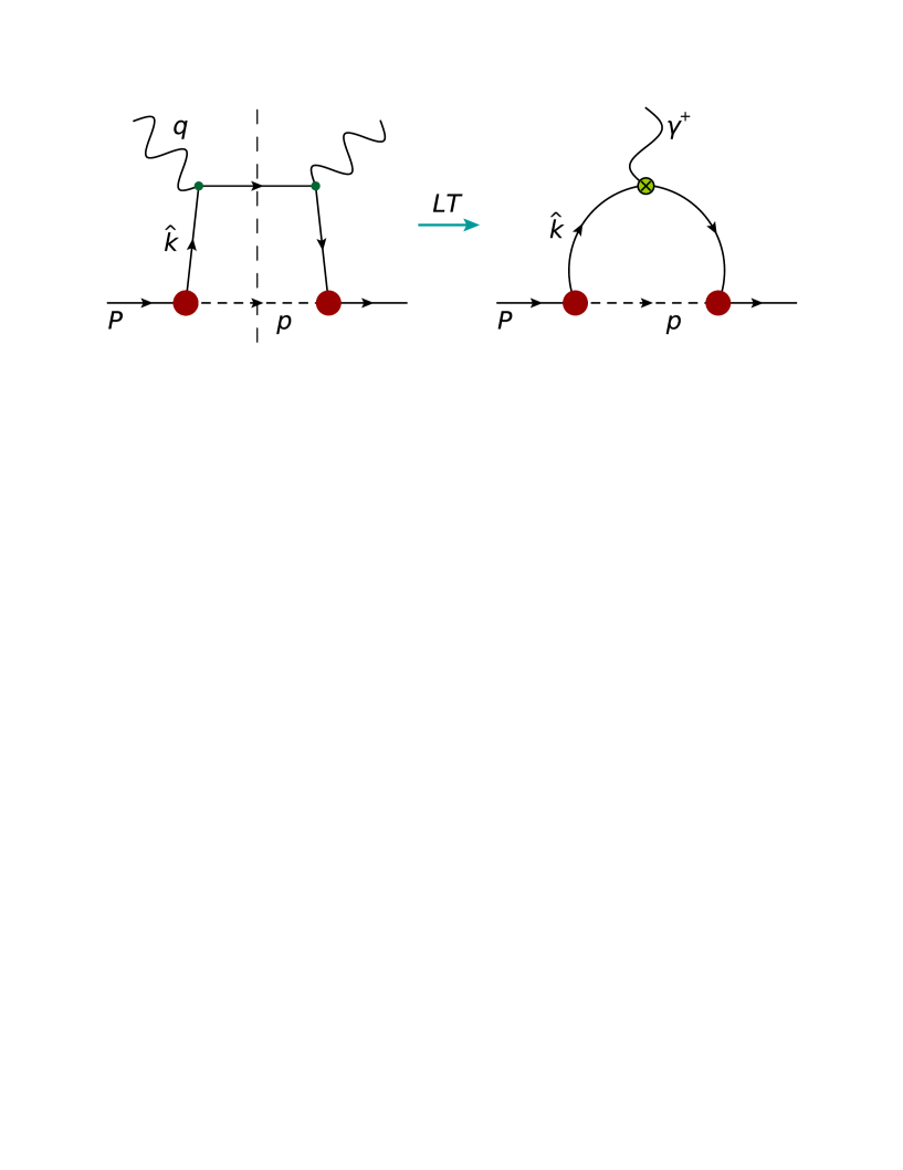
Figure 5: The leading twist (LT) reduction of the quark-level handbag diagram (left), to a form in which the quark-photon interaction enters explicitly via the $\gamma^{+}$ structure (right).

$\bar{c}$ in $D$

To model the distribution of a $\bar{c}$ quark in the pseudoscalar $D$ meson we consider the effective lagrangian describing the coupling of the $D$ to the $\bar{c}$ and a light quark $q$,

$${\cal L}_{\bar{c}qD} = ig\,\bar{\psi}_{\bar{c}}\,\gamma_{5}\,\psi_{q}\,\phi_{D}\ +\ \mathrm{h.c.}\ ,$$ (45)

where $\psi_{q}$ and $\psi_{\bar{c}}$ are the quark $q$ and $\bar{c}$ fields, and the effective coupling constant is now $g\to g_{\bar{c}qD}$. The contribution to the hadronic tensor of the $D$ meson from scattering off the $\bar{c}$ quark with a spectator light quark $q$ can be written in analogy with Eq. (21) for the hadronic calculation,

$$\bar{c}_{D}(z) = \frac{N_{D}}{16\pi^{2}}\int_{0}^{\infty}\frac{d\hat{k}^{2}_{\perp}}{z(1-z)}\frac{|G(\hat{s})|^{2}}{(m_{D}^{2}-\hat{s})^{2}}\,\widehat{T}^{\bar{c}q}\ ,$$ (46)

where $\hat{k}_{\perp}$ denotes the internal quark transverse momentum in the $D$ meson and $z$ is the Bjorken scaling variable for the quark inside the $D$ meson. Note that the total invariant mass squared of the $\bar{c}q$ pair is defined [see also Eq. (8)] for the corresponding invariant mass of the meson–baryon system) as

$$\hat{s}(z,\hat{k}^{2}_{\perp})=\frac{m_{\bar{c}}^{2}+\hat{k}^{2}_{\perp}}{z}+\frac{m_{q}^{2}+\hat{k}^{2}_{\perp}}{1-z}\ ,$$ (47)

where $m_{\bar{c}}$ is the constituent anticharm quark mass, $m_{q}$ is the mass of the (light) spectator quark.

The trace factor $\widehat{T}^{\bar{c}q}$ can then be computed from the quark-level “handbag” diagram, yielding

$$\widehat{T}^{\bar{c}q} = \frac{1}{4\hat{k}^{+}}\mathrm{Tr}\left[i\gamma_{5}(\hat{\not{k}}+m_{\bar{c}})\,\gamma^{+}\,(\hat{\not{k}}+m_{\bar{c}})\,(-i\gamma_{5})(-\hat{\not{p}}+m_{q})\right]\ ,$$ (48)

$$= 2\,\big{(}\hat{p}\cdot\hat{k}+m_{\bar{c}}m_{q}\big{)}\ ,$$

which follows from the on-mass-shell condition in time-ordered perturbation theory, $\hat{k}^{2}=m^{2}_{\bar{c}}$, with $\hat{p}$ the $4$-momentum of the spectator quark. Following the replacement shown in Fig. 5, the $\gamma^{+}$ structure arises from reducing the hard scattering amplitude to its leading twist approximation [210],

$$\gamma^{\mu}(\hat{\not{k}}+\not{q}+m_{\bar{c}})\gamma^{\nu}\,\,\delta\left([\hat{k}+q]^{2}-m_{\bar{c}}^{2}\right)\,\rightarrow\,{\gamma^{+}\over 2\hat{k}^{+}}\,\,\delta\left(1-{z\over\hat{y}}\right)\ ,$$ (49)

where $\hat{y}$ is the parton fraction of the hadron momentum, after equating the coefficients of $g^{\mu\nu}$ and selecting the $+$ component of the external photon current.

The result for $\bar{c}_{D}(z)$ is then obtained by inserting the expression for $\widehat{T}^{\bar{c}q}$ in Eq. (48) into Eq. (46), and using the IMF momenta as in Eq. (22) but with the replacements $y\to z$, $M\to M_{D}$, $m_{D}\to m_{\bar{c}}$, and $M_{B}\to m_{q}$. This yields the desired distribution of a relativistic $\bar{c}$ quark in a pseudoscalar $D$ meson, with a spectator $u$ or $d$ quark, in analogy with the $p\to D\Lambda_{c}$ splitting function in Eq. (26). Specifically, the manipulations of Eq. (48) demonstrate that using a pseudoscalar meson–quark–antiquark vertex parametrized by the structure $\gamma_{5}G(\hat{s})$, where $G(\hat{s})$ is the $D$-$\bar{c}$-$q$ vertex function ($q=u,d$), gives the distribution

$$\bar{c}_{D}(z) = \frac{N_{D}}{16\pi^{2}}\int_{0}^{\infty}\frac{d\hat{k}_{\perp}^{2}}{[z(1-z)]^{2}}\frac{|G(\hat{s})|^{2}}{(\hat{s}-m_{D}^{2})^{2}}\Big{[}\hat{k}^{2}_{\perp}+(z\,m_{q}+(1-z)\,m_{\bar{c}})^{2}\Big{]}\ ,$$ (50)

in which the integration is over the transverse momentum $\hat{k}_{\perp}^{2}$ of the interacting heavy quark, and $z$ is the Bjorken scaling variable of the heavy quark inside the charmed hadron. Here and in the following computations, the overall normalization $N_{D}$ is determined by the valence condition,

$$\int_{0}^{1}dz\,\bar{c}_{D}(z)=1\ .$$ (51)

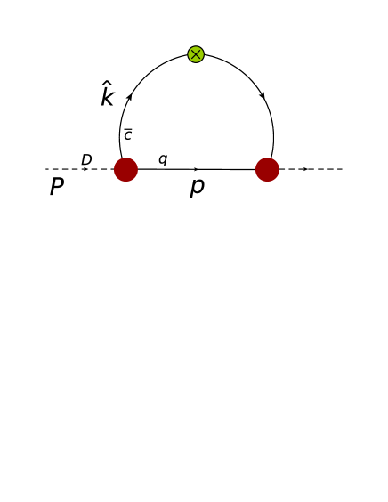
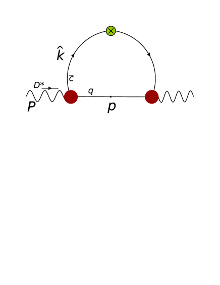
Figure 6: Diagrams for anticharm quark distributions inside charmed mesons.

$\bar{c}$ in $D^{*}$

For the $\bar{c}$ distribution in a vector $D^{*}$ meson, there exist in principle both the Dirac and Pauli couplings of the $D^{*}$ to a quark and antiquark, as for the $D^{*}B$ splitting function in Eq. (35). To reduce the number of free parameters in the calculation, we make the simplifying assumption that the $D^{*}$–quark–antiquark coupling is governed by a purely vector interaction, $\gamma_{\alpha}\,G(\hat{s})$. The result is that the following simple vector form is chosen for the lagrangian describing the $\bar{c}qD^{*}$ interaction,

$${\cal L}_{\bar{c}qD^{*}} = g\,\bar{\psi}_{\bar{c}}\,\gamma_{\mu}\,\psi_{q}\,\theta_{D^{*}}^{\mu}\ +\ \mathrm{h.c.}\ ,$$ (52)

where $g\to g_{D^{*}\bar{c}q}$. This yields the trace factor

$$\widehat{T}^{(\bar{c}q)^{*}} = \frac{1}{4\hat{k}^{+}}\mathrm{Tr}\left[(-\hat{\not{p}}+m_{q})\gamma^{\alpha}(\hat{\not{k}}+m_{\bar{c}})\,\gamma^{+}\,(\hat{\not{k}}+m_{\bar{c}})\,\gamma^{\beta}\right]\widetilde{g}_{\alpha\beta}$$ (53)

$$= 4\left(\frac{(P\cdot\hat{p})(P\cdot\hat{k})}{m_{D^{*}}^{2}}+\frac{3}{2}m_{\bar{c}}\,m_{q}+\frac{\hat{p}\cdot\hat{k}}{2}\right)\ .$$

Applying the same procedure as for the $\bar{c}$ distribution inside the pseudoscalar $D$ meson, one immediately arrives at the distribution of a $\bar{c}$ quark in the $D^{*}$ meson, which is given by

$$\bar{c}_{D^{*}}(z) = \frac{N_{D^{*}}}{16\pi^{2}}\int_{0}^{\infty}\frac{d\hat{k}_{\perp}^{2}}{[z(1-z)]^{2}}\frac{|G(\hat{s})|^{2}}{(\hat{s}-m_{D^{*}}^{2})^{2}}\Biggl{[}\left(\frac{\hat{k}^{2}_{\perp}+m_{q}^{2}}{m_{D^{*}}^{2}}+(1-z)^{2}\right)\left(\hat{k}^{2}_{\perp}+m_{\bar{c}}^{2}+z^{2}\,m_{D^{*}}^{2}\right)$$ (54)

$$\hskip 85.35826pt+\ \hat{k}^{2}_{\perp}\ +\ \left(z\,m_{q}+(1-z)\,m_{\bar{c}}\right)^{2}\ +\ 4z(1-z)\,m_{q}m_{\bar{c}}\Biggr{]}\ ,$$

with the normalization factor $N_{D^{*}}$ again determined by the valence quark number conservation condition in Eq. (51). As with the $\bar{c}$ distribution in the $D$ meson, for point interactions the integral in Eq. (54) would be divergent, in this case linearly in $\hat{k}_{\perp}^{2}$. This behavior can be controlled with vertex form factors $G(\hat{s})$ as we shall discuss in greater detail in Sec. 2.

$c$ in $\Lambda_{c}$, $\Sigma_{c}$

The charm quark distributions inside charmed baryons are obtained from an expression analogous to that in Eq. (46),

$$c_{B}(z) = \frac{N_{B}}{16\pi^{2}}\int_{0}^{\infty}\frac{d\hat{k}^{2}_{\perp}}{z(1-z)}\frac{|G(\hat{s})|^{2}}{(m_{B}^{2}-\hat{s})^{2}}\,\widehat{T}^{c[qq]}\ ,$$ (55)

where $\widehat{T}^{c[qq]}$ is the corresponding trace factor for the scattering from the $c$ quark with a spectator diquark $[qq]$ in the intermediate state. For spin-$1/2$ baryons, we consider the scalar interaction between the $c$ and $[qq]$ quarks and the charmed baryon, given by the lagrangian

$${\cal L}_{c[qq]B} = g\,\bar{\psi}_{B}\,\psi_{c}\,\phi_{[qq]}\ +\ \mathrm{h.c.}\ ,$$ (56)

with $g\to g_{c[qq]B}$, and $\phi_{[qq]}$ is the field of the scalar diquark. The trace factor $\widehat{T}^{c[qq]}$ can be explicitly derived from the left diagram of Fig 7 as

$$\widehat{T}^{c[qq]} = \frac{1}{4\hat{k}^{+}}\mathrm{Tr}\left[(\not{P}+M_{B})(\hat{\not{k}}+m_{c})\gamma^{+}(\hat{\not{k}}+m_{c})\right]$$ (57)

$$= 2\left(P\cdot\hat{k}+m_{c}\,M_{B}\right)\ ,$$

giving the net result for the charm quark distribution inside a spin-$1/2$ baryon $B$ ($B=\Lambda_{c}$ or $\Sigma_{c}$) with a scalar $qq$ spectator:

$$c_{B}(z) = \frac{N_{B}}{16\pi^{2}}\int_{0}^{\infty}\frac{d\hat{k}_{\perp}^{2}}{z^{2}(1-z)}\frac{|G(\hat{s})|^{2}}{(\hat{s}-M_{B}^{2})^{2}}\Big{[}\hat{k}^{2}_{\perp}+(m_{c}+zM_{B})^{2}\Big{]}\ ,$$ (58)

where for the charm quark mass we take $m_{c}=m_{\bar{c}}$, and the invariant mass squared of the quark–diquark system here is defined as

$$\hat{s}(z,\hat{k}^{2}_{\perp})=\frac{m_{c}^{2}+\hat{k}^{2}_{\perp}}{z}+\frac{m_{qq}^{2}+\hat{k}^{2}_{\perp}}{1-z}\ .$$ (59)

The functional form of the $B$-$c$-$qq$ vertex function $G(\hat{s})$ will be specified as for the $D$-$\bar{c}$-$q$ function in the phenomenological schemes to be outlined in Sec. 2, and the normalization constant $N_{B}$ is now determined from an analogous valence charm quark number condition to that in Eq. (51),

$$\int_{0}^{1}dz\,c_{B}(z)=1\ .$$ (60)

Note that for the $\Sigma_{c}^{++}$ baryon, the $uu$ spectator diquark has spin 1, so that the calculation of its $c$ quark distribution here is approximated by neglecting the diquark’s spin structure. In principle, it is straightforward to include both spin-0 and spin-1 diquark contributions in analogy with the spin structures discussed for the anticharm distributions; however, because the overall contribution from the dissociation of the proton to $D^{-}\Sigma_{c}^{++}$ is at least an order of magnitude smaller than for $\bar{D}^{*0}\Lambda_{c}^{+}$, this will have negligible effect on the numerical results.

$c$ in $\Sigma_{c}^{*}$

Lastly, for the charm density of the spin-$3/2$ $B^{*}$ baryons we adopt the following lagrangian,

$${\cal L}_{c[qq]^{*}B^{*}} = \frac{g}{m_{[qq]^{*}}}\ i\left(\bar{\Psi}_{B^{*}\nu}\gamma_{\mu}\psi_{c}-\bar{\psi}_{c}\gamma_{\mu}\Psi_{B^{*}\nu}\right)F_{[qq]^{*}}^{\mu\nu}\ ,$$ (61)

with $g\to g_{c[qq]^{*}B^{*}}$, which correctly gives the parities of the physical $B^{*}$ and quark fields. Again, the field strength tensor here has the form $F_{[qq]^{*}}^{\mu\nu}=\partial^{\mu}\theta_{[qq]^{*}}^{\nu}-\partial^{\nu}\theta_{[qq]^{*}}^{\mu}$, where $\theta_{[qq]^{*}}$ denotes the (spin-1) axial-vector diquark. The trace factor in this case is found to be

$$\widehat{T}^{c[qq]^{*}} = \frac{1}{4m^{2}_{[qq]^{*}}\hat{k}^{+}}\mathrm{Tr}\left[\Lambda_{B^{*}}^{\beta^{\prime}\alpha^{\prime}}(P)\gamma^{\alpha}(\hat{\not{k}}+m_{c})\,\gamma^{+}\,(\hat{\not{k}}+m_{c})\gamma^{\beta}\right]\mathcal{G}_{\alpha\beta\alpha^{\prime}\beta^{\prime}}\ .$$ (62)

After re-indexing, $\mathcal{G}_{\alpha\beta\alpha^{\prime}\beta^{\prime}}$ is given by Eq. (42), the exchange boson carries the $4$-momentum $\hat{\Delta}=P-\hat{k}$, and the metric tensor of the massive, spin-1 diquark is $\widetilde{g}^{\mu\nu}=-g^{\mu\nu}+P^{\mu}P^{\nu}/m^{2}_{[qq]^{*}}$. Computing the trace and contractions of Eq. (62) and evaluating the result with the appropriate kinematic definitions analogous to Eq. (22), the charm distribution in spin-3/2 $\Sigma_{c}^{*}$ baryons emerges. Here, the charm quark is always accompanied by a spin-1 diquark, such that after incorporating the fully relativistic Rarita-Schwinger structure for the spin-3/2 state, the charm quark distribution in the $\Sigma_{c}^{*}$ is given by

$$c_{B^{*}}(z) = \frac{N_{B^{*}}}{12\pi^{2}m_{qq}^{2}}\int_{0}^{\infty}\frac{d\hat{k}_{\perp}^{2}}{z(1-z)}\frac{|G(\hat{s})|^{2}}{(\hat{s}-M_{B^{*}}^{2})^{2}}\Biggl{(}(\hat{k}\cdot\hat{\Delta})(P\cdot\hat{\Delta})+2m_{c}M_{B^{*}}\hat{\Delta}^{2}$$

$$+ \frac{1}{m_{qq}^{2}}\Bigl{[}m_{c}M_{B^{*}}(\hat{p}\cdot\hat{\Delta})^{2}-(\hat{p}\cdot\hat{\Delta})\Bigl{(}(\hat{p}\cdot\hat{\Delta})(\hat{k}\cdot\hat{p})-(P\cdot\hat{\Delta})(\hat{k}\cdot\hat{p})-(\hat{k}\cdot\hat{\Delta})(P\cdot\hat{p})\Bigr{)}$$

$$- (P\cdot\hat{p})(\hat{k}\cdot\hat{p})\hat{\Delta}^{2}-\frac{P\cdot\hat{k}}{M_{B^{*}}^{2}}\Bigr{(}(P\cdot\hat{p})^{2}\hat{\Delta}^{2}-m_{qq}^{2}(P\cdot\hat{\Delta})^{2}-2(P\cdot\hat{\Delta})(\hat{p}\cdot\hat{\Delta})(P\cdot\hat{p})\Bigr{)}\Bigr{]}\Biggr{)}\ ,$$

in which $\hat{p}$ is the momentum of the spectator diquark $qq$, and $\hat{\Delta}\equiv P-\hat{k}$ [see Eq. (22)].

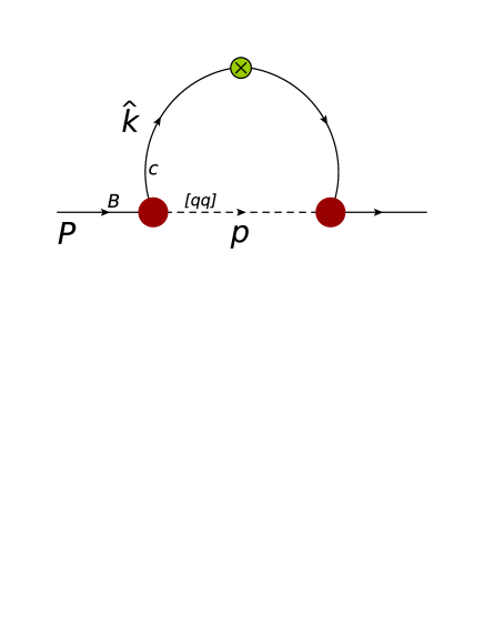
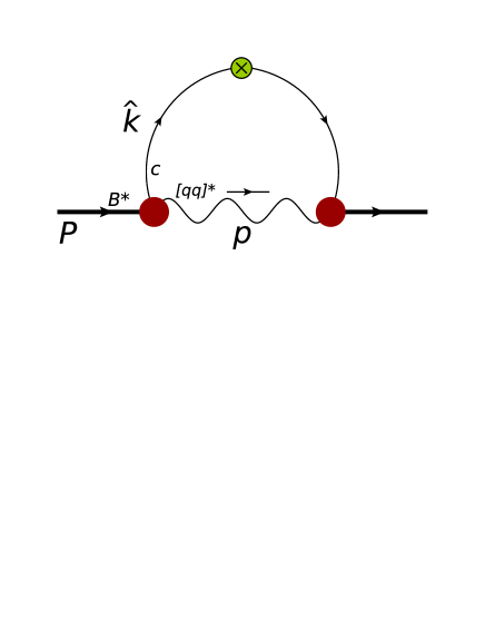
Figure 7: Diagrams for anticharm quark distributions inside baryons.

1 Hadronic Probability Distributions

Thus, for a given meson–baryon state $MB$, the splitting function can be evaluated as in Eq. (11) in terms of an integral over the transverse momentum of the square of the probability amplitude $\phi_{BM}(y,k^{2}_{\perp})$ which was defined in Eq. (7). The desired probability amplitudes can then be taken from time-ordered perturbation theory as we have just done at the start of Sec. 2.

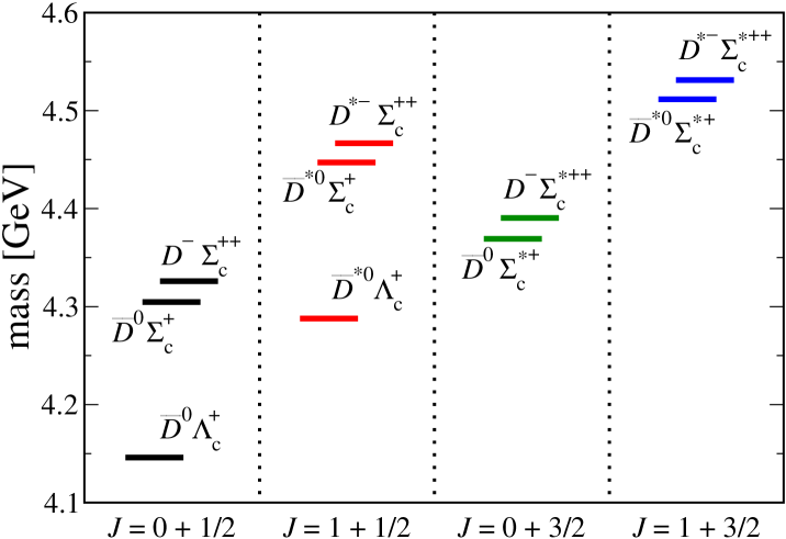
Figure 8: Spin configurations ($J=$ meson + baryon spin) and masses for the spectrum of charmed hadron configurations included in the present MBM calculation.

The full model is generated from an incoherent sum over the various states detailed in Table 1 and illustrated in Fig. 8 (with the exception of the $p\,J/\psi$ state). In particular, this requires all the hadronic splitting functions derived above for $p\to MB$ fluctuations in the spin transitions

$$\bm{\frac{1}{2}}\ \ \ \rightarrow\ \ \ \bm{0}\bigoplus\bm{\frac{1}{2}},\ \ \ \bm{1}\bigoplus\bm{\frac{1}{2}},\ \ \ \bm{0}\bigoplus\bm{\frac{3}{2}},\ \ \ \bm{1}\bigoplus\bm{\frac{3}{2}}\ .$$ (64)

We take numerical values for the couplings to each of these states from the lowest-order effective hadronic lagrangian for each transition as we describe momentarily, after a brief discussion of the phenomenology of the vertex calculation.

Vertex regularization.

At large transverse momenta, the invariant mass goes like $s\sim k_{\perp}^{2}$, making integrals of the type given in Eq. (26) logarithmically divergent. A simple way to regulate these divergences is through wave function suppression factors $F(s)$, which act to dampen the ultraviolet contributions. If we make the reasonable assumption that the quark model symmetries used to fix the hadronic coupling constants $g$ (discussed below) are not strongly broken, the scheme used to regulate these transverse divergences is is in fact the primary source of model dependence. The ambiguity as to which choice of functional form, etc., is most appropriate has led to a diverse collection of approaches, many of which possess unique numerical and phenomenological advantages.

Throughout the present analysis, we use an especially convenient parametrization in the form of an exponential function of $s$,

$$F(s)=\exp[-(s-M^{2})/\Lambda^{2}]\ ,$$ (65)

which has the merit of possessing simple normalization properties on-shell, although multipole, or power-law, functional forms as in Eq. (6) would also suffice.

Moreover, as we catalogued in Sec. 2, both the hadronic and quark-level amplitudes are evaluated in an IMF/light front framework; at the same time, in an explicitly covariant formulation, $t$-channel parametrizations of the form factor may possess more general consistency. Such a prescription specifies the splitting functions directly in terms of the Mandelstam variable $t=-k^{2}$ (here, the exchanged mass of the virtual meson), leading to, e.g.,

$$f_{MB}(y)={c_{I}\,g^{2}_{MBN}\over 16\pi^{2}}\,\,y\int_{t_{min}}^{\infty}dt\left(t+[M_{B}-M]^{2}\over(t+m_{M}^{2})^{2}\right)\,\,F^{2}(t)\ ,$$ (66)

for the simplest pseudoscalar process $p\rightarrow MB$, corresponding to Eq. (26). Typical choices for vertex suppression then usually involve multipole forms such as

$$F(t)=\left(\Lambda^{2}+m_{M}^{2}\over\Lambda^{2}-t\right)^{n}\ ,\,\,\,\,n\in\{1,\,2\}\ .$$ (67)

Despite the frame-independence conferred by the covariant approach, several shortfalls of this method prevent us from using it extensively here; perhaps the greatest of these is the explicit lack of symmetry between scattering and recoil processes typified by the $y\rightarrow\bar{y}\equiv 1-y$ reciprocity relation of Eq. (11), which prevails in the IMF framework. As we have seen, this property in the IMF enforces $3$-momentum conservation in interactions determined by the effective $\mathcal{L}_{MBN}$ of Sec. 2. It can be shown, however, that $f_{MB}(y)\neq f_{BM}(\bar{y})$ in amplitudes like those of Eqs. (66 & 67) — a fact which implies that covariant schemes generally fail to uphold explicit momentum conservation at hadronic vertices.

As mentioned, the splitting functions also depend upon the magnitude of the coupling $g$ to each meson–baryon state, which we take from baryon–baryon scattering models extended to the charm sector. For simplicity, we assume a universal exponential form factor for all couplings, where the resulting scale factor $\Lambda$ is varied to fit charmed baryon production in hadronic interactions, as discussed below. (Note that the exponential expression used to define $F(s)$ in Eq. (65) differs by the square of the form factor appearing in Eq. (5); the two can of course be related by a simple rescaling of the cutoff mass $\Lambda^{2}\to 2\Lambda^{2}$.)

Constraints from inclusive charmed hadron production.

To calculate the contributions of the various charmed mesons and baryons listed in Table 1 requires the couplings of these states to the proton. In this analysis we take the coupling constants from boson-exchange models that were originally applied to pion-nucleon interactions [200], and later generalized to $KN$ scattering [201]. In the extension to the strange sector, the relevant couplings are taken from non-strange analyses with SU(3) arguments used to incorporate the corresponding strange particles. The off-shell behavior of the amplitudes is typically regulated by a multipole form factor of the type

$$F(t)=\left(\frac{\Lambda^{2}+m_{M}^{2}}{\Lambda^{2}-t}\right)^{n}\ ,$$ (68)

where $t$ is the usual Mandelstam variable for the squared momentum transfer of the exchanged meson with mass $m_{M}$. A monopole form factor ($n=1$) is most often used for low-spin states, while for higher-spin states a dipole form factor ($n=2$) is typically employed to damp the higher powers of momentum that enter into the transition amplitudes.

The extension of meson–baryon couplings from the non-strange to the strange sector has generally been quite successful phenomenologically. Continuing this program further to the charm sector, Haidenbauer et al. [187, 188, 189] used SU(4) symmetry arguments to describe exclusive charmed hadron production in $\bar{D}N$ and $DN$ scattering within a one-boson-exchange framework. We fix the couplings for the spin-1/2 charmed baryons $\Lambda_{c}$ and $\Sigma_{c}$ to those found in Ref. [189], as summarized in Table 2. For the couplings to spin-3/2 states $\Sigma_{c}^{*}$, we take the couplings from those obtained for the analogous strange states by Holzenkamp et al. [202]. The signs of the couplings are related to the value of the $\pi NN$ coupling, for which we use $g_{\pi NN}/\sqrt{4\pi}=-3.795$.

Table 2: Charm-sector coupling constants, deduced from $DN$ and $\bar{D}N$ scattering analyses [189] for the spin-1/2 charmed baryons $\Lambda_{c}$ and $\Sigma_{c}$, and by extending the SU(3) sector analysis of Ref. [202] for the spin-3/2 $\Sigma_{c}^{*}$ states.

Vertex	$g_{MBN}/\sqrt{4\pi}$	$f_{MBN}/\sqrt{4\pi}$
$p\to\bar{D}^{0}\Lambda_{c}^{+}$	3.943	—
$p\to\bar{D}^{*0}\Lambda_{c}^{+}$	1.590	5.183
$p\to\bar{D}^{0}\Sigma_{c}^{+},\ D^{-}\Sigma_{c}^{++}$	0.759	—
$p\to\bar{D}^{*0}\Sigma_{c}^{+},\ D^{*-}\Sigma_{c}^{++}$	0.918	$-2.222$
$p\to\bar{D}^{0}\Sigma_{c}^{*+},\ D^{-}\Sigma_{c}^{*++}$	$-0.193$	—
$p\to\bar{D}^{*0}\Sigma_{c}^{*+},\ D^{*-}\Sigma_{c}^{*++}$	$-1.846$	—

The remaining parameters of the model are the form factor cutoffs, $\Lambda$, which could in principle be constrained for the various meson–baryon vertices by data from exclusive or inclusive charmed baryon production. In practice, such data are rather limited, and the most direct constraints come from inclusive $\Lambda_{c}$ production in proton–proton scattering, $pp\to\Lambda_{c}X$, measured by the R680 Collaboration at the ISR [191]. Since it is currently not possible to constrain the cutoffs for the individual charmed meson–baryon configurations, we assume a universal exponential form factor cutoff as in Eq. (65) for all the fluctuations listed in Table 2, and tune $\Lambda$ to best reproduce the shape and normalization of the inclusive $\Lambda_{c}$ production cross section data. This will place an upper bound on $\Lambda$ and the magnitude of the charmed meson–baryon contribution in the MBM.

Within the same one-boson exchange framework as adopted in the $DN$ and $\bar{D}N$ scattering analyses [187, 188, 189], the contribution from charmed meson exchange to the differential cross section for inclusive baryon production in $pp$ scattering can be written [195]

$$E\frac{d^{3}\sigma}{d^{3}\bm{p}}\ =\ \frac{\bar{y}}{\pi}\frac{d^{2}\sigma}{d\bar{y}\,dk_{\perp}^{2}}\ =\ \frac{\bar{y}}{\pi}\sum_{M}\left|\phi_{BM}(\bar{y},k_{\perp}^{2})\right|^{2}\,\sigma_{\rm tot}^{Mp}(sy)\ ,$$ (69)

where $E$ is the energy of the proton beam, and the sum over $M$ includes incoherent contributions from processes involving the exchange of meson $M$ leading to a final baryon $B$. The total meson–proton cross section $\sigma_{\rm tot}^{Mp}$ here is evaluated at the meson energy $sy$, with $s$ being the total $pp$ invariant mass squared. For the case of $\Lambda_{c}^{+}$ production, the sum is restricted to the $\bar{D}^{0}$ and $\bar{D}^{*0}$ mesons. The $k_{\perp}^{2}$-integrated cross section for $\Lambda_{c}^{+}$ production is then given by

$$\frac{d\sigma}{d\bar{y}}=\sum_{M=D,D^{*}}f_{\Lambda_{c}^{+}M}(\bar{y})\,\sigma_{\rm tot}^{Mp}(sy)\ .$$ (70)

Note that in Ref. [203] this cross section is defined with an additional factor $(\pi/\bar{y})$ on the right hand side. For the total charmed meson–proton cross section $\sigma_{\rm tot}^{Mp}$ we take a constant value, as suggested by the analysis of pion-nucleon scattering [195], where $\sigma_{\rm tot}^{\pi p}\approx\sigma_{\rm tot}^{\rho p}$. Adopting a similar approach to the strange and charmed meson cross sections, we have

$$\sigma_{\rm tot}^{Dp}\ \approx\ \sigma_{\rm tot}^{D^{*}p}\ \approx\ \sigma_{\rm tot}^{\bar{K}p}\ \approx\ (20\pm 10)\ \mathrm{mb}\ ,$$ (71)

where the value of the $\bar{K}p$ total cross section is taken from Ref. [22], and we assign a conservative 50% uncertainty on the central value.

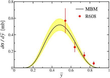
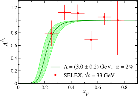
Figure 9: (Left) Differential cross section $d\sigma/d\bar{y}$ for the inclusive charm production reaction $pp\to\Lambda_{c}^{+}X$ as a function of the momentum fraction $\bar{y}$ carried by the $\Lambda_{c}^{+}$. The MBM cross section (solid) is computed using the central value for the $Dp$ cross section $\sigma^{Dp}_{\rm tot}=20$ mb, and the resulting error band (shaded) represents the purely statistical uncertainty. The data (red circles) are from the R608 collaboration at the ISR [191]. (Right) Charge asymmetry $A^{\Lambda_{c}}$ for $\Lambda_{c}^{+}/\bar{\Lambda}_{c}^{-}$ production in the MBM (solid), using the ${x_{{\scriptscriptstyle F}}}$ dependence of the $\bar{\Lambda}_{c}$ cross section in Eq. (74), compared with data from the SELEX Collaboration [192].

Using Eqs. (70) and (71), the calculated cross section is shown in the left-hand panel of Fig. 9 at the kinematics of the $\Lambda_{c}^{+}$ production data from the R608 Collaboration [191] at the ISR. The kinematical coverage of the ISR data was restricted to $k_{\perp}\leq 1.1$ GeV, which we impose in the computed cross section. For the central value of the $Dp$ total cross section, $\sigma_{\rm tot}^{Dp}=20$ mb, the best fit value of the cutoff parameter is found to be $\Lambda=(2.89\pm 0.04)$ GeV, which gives a good fit to both the overall normalization and the shape of the inclusive $\Lambda_{c}^{+}$ data. Including the uncertainty in the $Dp$ cross section from Eq. (71), the cutoff becomes $\Lambda=(3.0\pm 0.2)$ GeV.

In calculating the inclusive $\Lambda_{c}^{+}$ production cross section we have included the possibility that higher-mass baryons such as $\Lambda_{c}^{*}$ and $\Sigma_{c}^{*}$ are produced and subsequently decay to a $\Lambda_{c}^{+}$, using the relevant branching ratios for the decays. With the coupling constants from Table 2, we find that the dominant contribution to inclusive $\Lambda_{c}$ production arises from the state $\bar{D}^{*0}\Lambda_{c}^{+}$. This is in contrast to earlier analyses, where the largest contribution was assumed to be from the lowest-energy $\bar{D}^{0}\Lambda_{c}^{+}$ state. As we discuss below, this will have significant ramifications for intrinsic charm production in electromagnetic reactions.

We must point out that the original data from Ref. [191] were recorded in terms of the variable ${x_{{\scriptscriptstyle F}}}=2p_{\Lambda}^{0}/\sqrt{s}$, which in general differs from the momentum fraction $\bar{y}$ that scales the calculations of the MBM. It can be shown, however, that at high energies (i.e., $s\gg M_{B}^{2}$, $k_{\perp}^{2}$), one has $\bar{y}\to{x_{{\scriptscriptstyle F}}}$, which we used to create the abscissa of the left panel in Fig. 9.

Somewhat more recently the SELEX Collaboration at Fermilab [192] produced data on the charge asymmetry for inclusive $\Lambda_{c}^{+}$ and $\bar{\Lambda}_{c}^{-}$ production in the scattering of 540 GeV protons from copper and carbon targets,

$$A^{\Lambda_{c}}({x_{{\scriptscriptstyle F}}})={\sigma^{\Lambda_{c}}(x_{F})-\sigma^{\bar{\Lambda}_{c}}(x_{F})\over\sigma^{\Lambda_{c}}(x_{F})+\sigma^{\bar{\Lambda}_{c}}(x_{F})}\ ,$$ (72)

where $\sigma^{\Lambda_{c}}(x_{F})\equiv d\sigma^{\Lambda_{c}}/d{x_{{\scriptscriptstyle F}}}$. While the contribution to the production of $\Lambda_{c}^{+}$ can be calculated in the MBM, the computation of the asymmetry $A^{\Lambda_{c}}$ requires in addition an estimate of the $\bar{\Lambda}_{c}$ cross section. Following Ref. [192] we approximate this using a simple monomial parametrization. Furthermore, we assume that the $\Lambda_{c}^{+}$ cross sections can be written as the sum of valence and sea components, with the generation of the former described by the nonperturbative MBM and dominating at intermediate and high values of ${x_{{\scriptscriptstyle F}}}$, and the latter concentrated at small ${x_{{\scriptscriptstyle F}}}$,

$$\frac{d\sigma^{\Lambda_{c}}}{d{x_{{\scriptscriptstyle F}}}}=\frac{d\sigma^{\Lambda_{c}}_{\rm(val)}}{d{x_{{\scriptscriptstyle F}}}}+\frac{d\sigma^{\Lambda_{c}}_{\rm(sea)}}{d{x_{{\scriptscriptstyle F}}}}\ ,$$ (73)

where

$$\frac{d\sigma^{\Lambda_{c}}_{\rm(val)}}{d{x_{{\scriptscriptstyle F}}}} \approx \sigma_{0}\sum_{M}f_{\Lambda_{c}M}({x_{{\scriptscriptstyle F}}})\ ,$$ (74a)

$$\frac{d\sigma^{\Lambda_{c}}_{\rm(sea)}}{d{x_{{\scriptscriptstyle F}}}} \equiv \frac{d\sigma^{\bar{\Lambda}_{c}}}{d{x_{{\scriptscriptstyle F}}}}\ \approx\ \bar{\sigma}_{0}(1-{x_{{\scriptscriptstyle F}}})^{\bar{n}}\ .$$ (74b)

In Eq. (74a) the factor $\sigma_{0}$ corresponds to the total meson–proton cross section in Eq. (70), which we take to be independent of the flavor and spin of the meson, as in Eq. (71), while $\bar{\sigma}_{0}$ is a normalization parameter for the corresponding $\bar{\Lambda}_{c}$ production cross section. Using Eqs. (74), the asymmetry in Eq. (72) can then be written

$$A_{\Lambda_{c}}({x_{{\scriptscriptstyle F}}})=\frac{\sum_{M}f_{\Lambda_{c}M}({x_{{\scriptscriptstyle F}}})}{\sum_{M}f_{\Lambda_{c}M}({x_{{\scriptscriptstyle F}}})+2\alpha(1-{x_{{\scriptscriptstyle F}}})^{\bar{n}}}\ ,$$ (75)

where $\alpha=\bar{\sigma}_{0}/\sigma_{0}$ is the ratio of the sea to valence contributions to the $\Lambda_{c}$ cross sections. For $\bar{\Lambda}_{c}$ production induced by $\Sigma^{-}$ beams, the SELEX Collaboration found for the exponent $\bar{n}\approx 6.8$, which we assume also for the $x_{F}$ dependence of the proton induced cross section in Eq. (74b). Using the MBM cutoff parameter $\Lambda=(3.0\pm 0.2)$ GeV, a good fit to the SELEX charge asymmetry data can then be obtained with $\alpha\approx 2.0\%$, as displayed in the the right panel of Fig. 9. We should note, however, that $\Lambda_{c}$ charge asymmetry data are rather sensitive to the form of the $\bar{\Lambda}_{c}$ cross section, so that agreement with the SELEX data should not be considered as a stringent test of the MBM; rather, with an appropriate choice of parameter $\alpha$ the model is able to accommodate the empirical results. We therefore regard this reasonable description of SELEX data as a rough consistency argument on behalf of the MBM we have constructed, given the plausible behavior assumed for the sea contribution to $\Lambda_{c}$ production in Eq. (74b).

Having thus constrained the scale parameter for the meson–baryon form factor by the inclusive $\Lambda_{c}$ production data, and with the coupling constants for the various meson–baryon states given in Table 2, we are now able to compute the meson–baryon splitting functions in Eq. (11), which we consider in the following section.

Phenomenology of charmed meson–baryon splitting functions.

The complete set of the four basic splitting functions representing the dissociation of a proton to charmed meson–baryon states $p\to DB$ (pseudoscalar meson + octet baryon), $D^{*}B$ (vector meson + octet baryon), $DB^{*}$ (pseudoscalar meson + decuplet baryon) and $D^{*}B^{*}$ (vector meson + decuplet baryon) is illustrated in Fig. 10. The functions are shown for the neutral $\bar{D}^{0}$ and $\bar{D}^{*0}$ mesons, and all the other charge states in Table 2 can be obtained using appropriate Clebsch-Gordan coefficients. For the best fit value of the universal cutoff parameter $\Lambda=3$ GeV from the inclusive $\Lambda_{c}^{+}$ production data, the $\bar{D}^{*0}\Lambda_{c}^{+}$ contribution is found to be dominant — an order of magnitude larger than the corresponding $\bar{D}^{0}\Lambda_{c}^{+}$ and $\bar{D}^{*0}\Sigma_{c}^{*+}$ contributions. The $\bar{D}^{0}\Sigma_{c}^{*+}$ contribution is two orders of magnitude smaller still, and effectively plays no role in the phenomenology. To a good approximation, therefore, one can represent the total charm distribution in the proton by the single $\bar{D}^{*0}\Lambda_{c}^{+}$ state.

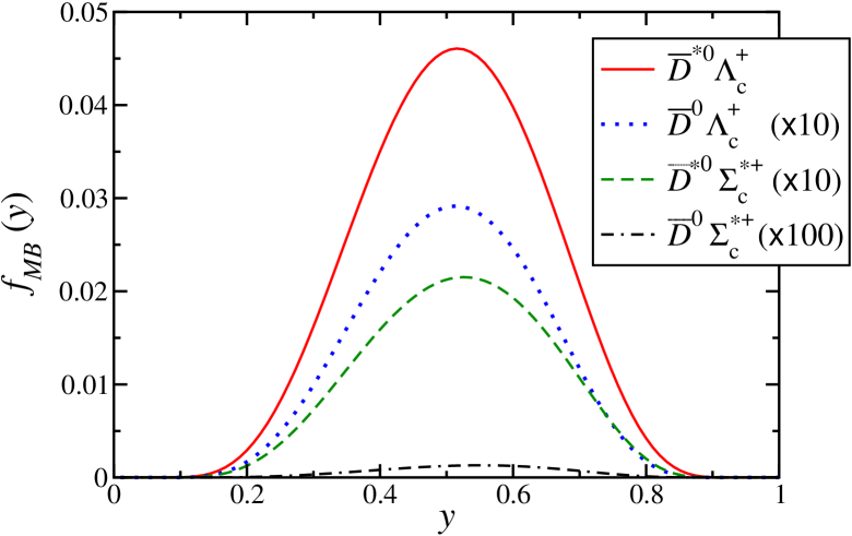
Figure 10: Splitting functions for the four basic dissociations of a proton into charmed meson–baryon states, for the spin-1 meson + spin-1/2 baryon state $\bar{D}^{*0}\Lambda_{c}^{+}$ (red solid), spin-0 meson + spin-1/2 baryon state $\bar{D}^{0}\Lambda_{c}^{+}$ (scaled $\times 10$, blue dotted), spin-1 meson + spin-3/2 baryon state $\bar{D}^{*0}\Sigma_{c}^{*+}$ (scaled $\times 10$, green dashed), and spin-0 meson + spin-3/2 baryon state $\bar{D}^{0}\Sigma_{c}^{*+}$ (scaled $\times 100$, black dot-dashed). A universal exponential cutoff mass $\Lambda=3$ GeV is used with the couplings from Table 2.

Again as indicated in Fig. 10, the shapes of the various charmed meson–baryon distributions $f_{MB}(y)$ are interestingly rather similar, peaking just above $y=1/2$. This is in contrast to the distributions in the light flavor sector, where the corresponding $\pi N$ splitting function is considerably more skewed in $y$ [194, 195]. The skewedness arises from the large difference in mass between the pion and nucleon in the dissociation, whereas the masses of both the charmed meson and baryon are of the order $\sim 2$ GeV. This is also one reason why the lowest mass $\pi N$ configuration is the dominant one in the pion sector (a fact to which we will return in Chap. 5), unlike the lowest mass charmed state $\bar{D}^{0}\Lambda_{c}^{+}$, which as Fig. 10 indicates gives a significantly smaller contribution than the $\bar{D}^{*0}\Lambda_{c}^{+}$. The dominance of the SU(2) flavor sector by the $\pi N$ state is ensured by the relatively large energy gap between higher mass configurations involving $\rho$ mesons or $\Delta$ baryons, whereas no significant energy gap exists between the various states in the charm sector.

To explore further the origin of the dominance of the $\bar{D}^{*0}\Lambda_{c}^{+}$ contribution, we note the relatively strong coupling to the vector meson state, particularly for the tensor coupling term, as seen in Table 2, where the tensor to vector coupling ratio is $f_{D^{*}\Lambda_{c}N}/g_{D^{*}\Lambda_{c}N}=3.26$ [187, 188, 189]. This is analogous to the large tensor coupling for the $\rho$ meson in one-boson exchange models of the $NN$ interaction [200], where in the Bonn-Jülich model, for instance, one has an even larger tensor/vector ratio, $f_{\rho NN}/g_{\rho NN}=6.1$ [204]. Using the charm couplings from Table 2, the tensor contribution clearly dominates over the vector term. This feature is preserved even if one uses the SU(2) couplings from the $\rho$ exchange in the $NN$ analysis instead of the SU(4) couplings [187, 188, 189] (but with the same charm hadron masses). In particular, since the SU(4) vector coupling $g_{D^{*}\Lambda_{c}N}^{2}/4\pi=2.53$ is around 5 times larger than that found for the $\rho$ from $NN$ analyses, $g_{\rho NN}^{2}/4\pi=0.55$ [204], the vector contribution to the charm splitting function is significantly larger than for the SU(2) coupling case. This is compensated somewhat by the $\sim 2$ times smaller SU(4) tensor/vector ratio, making the total contribution to the charmed vector meson splitting function $f_{\bar{D}^{*0}\Lambda_{c}^{+}}(y)$ similar.

At the effective lagrangian level, the large tensor contribution is associated with the additional momentum dependence induced by the derivative coupling in the tensor interaction, which is a general feature of couplings to states with higher spin [see Eq. (32)]. This additional momentum dependence can have a significant impact on the relative importance of various charmed meson–baryon transitions, as is evident from the form of the splitting function in Eq. (35). The effect of the momentum dependence of the meson–baryon vertices on the splitting functions can be illustrated even more dramatically by considering the normalizations $\langle n\rangle_{MB}=\int dy\,f_{MB}(y)$ as a function of the cutoff $\Lambda$. These are displayed in the left panel of Fig. 11 for the four charmed states shown in Fig. 10, together with the sum over all contributions. At the best fit value of $\Lambda\sim 3$ GeV, the lowest mass vector state $\bar{D}^{*0}\Lambda_{c}^{+}$ makes up around 70% of the total charm normalization of $\langle n\rangle_{MB}^{\rm(charm)}=2.40\%$. Including the uncertainty on the cutoff (indicated by the shaded band), the total charm normalization ranges from $\approx 1.04\%$ to $\approx 4.87\%$.

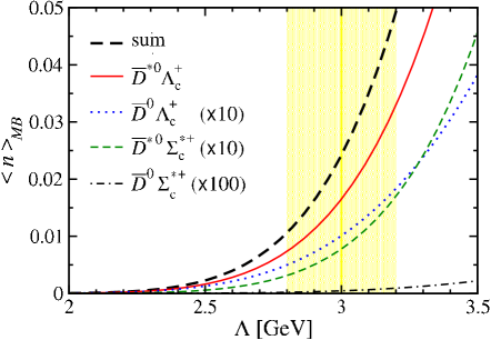
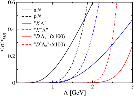
Figure 11: (Left) Normalizations $\langle n\rangle_{MB}$ of the charmed meson–baryon splitting functions as a function of the form factor cutoff $\Lambda$, for the states $\bar{D}^{*0}\Lambda_{c}^{+}$ (red solid), $\bar{D}^{0}\Lambda_{c}^{+}$ (scaled $\times 10$, blue dotted), $\bar{D}^{*0}\Sigma_{c}^{*+}$ (scaled $\times 10$, green dashed), and $\bar{D}^{0}\Sigma_{c}^{*+}$ (scaled $\times 100$, black dot-dashed), as well as the sum of all contributions (black dashed). The (yellow) shaded band represents the uncertainty on the cutoff obtained from fits to inclusive $\Lambda_{c}^{+}$ production data. (Right) Normalizations of the splitting functions to pseudoscalar (solid) and vector (dashed) mesons computed with SU(2) sector ($\pi N$ and $\rho N$) masses (black), SU(3) masses, denoted by “$K\Lambda$” and “$K^{*}\Lambda$” (blue), and SU(4) masses, denoted by “$D\Lambda_{c}$” and “$D^{*}\Lambda_{c}$” (scaled $\times 100$, red), all for the same SU(2) couplings.

While the variation of the charm splitting functions with the choice of SU(4) or SU(2) couplings is in reality relatively mild, a more significant effect is seen for the dependence of the splitting functions on the hadron masses. In Fig. 11(b) the normalizations $\langle n\rangle_{MB}$ of splitting functions to pseudoscalar and vector mesons are illustrated for the light-quark, strange and charmed sectors, using the SU(2) coupling constants for $\pi NN$ and $\rho NN$ listed above. The curves labeled “$K\Lambda$” and “$K^{*}\Lambda$” are obtained from the $\pi N$ and $\rho N$ splitting functions by replacing the pion and recoil baryon masses with the appropriate kaon and hyperon masses, and those labeled “$D\Lambda_{c}$” and those labeled “$D^{*}\Lambda_{c}$” are obtained by using the corresponding charmed meson and baryon masses. For small values of the cutoff, the normalizations of the pseudoscalar meson–baryon states is larger than for the vector meson states, but with increasing $\Lambda$ the contributions from the vector meson states eventually dominate. With increasing hadron masses the cross-over point between the pseudoscalar and vector meson states occurs at progressively smaller $\Lambda$ values. Neglecting differences between the coupling constants (which are small if quark model symmetries are assumed), the size of hadronic masses relative to the cutoff scale $\Lambda$ is the main determinant of the balance between the pseudoscalar and vector states for a given flavor sector.

The best fit value $\Lambda=3$ GeV for the charmed splitting functions corresponds to a region where the vector meson term clearly dominates over the pseudoscalar meson contribution. Had we found a significantly softer cutoff $\Lambda\sim 1$ GeV, the pseudoscalar contribution would have dominated, although for such values the total charm contribution would be negligible. Since only a single charmed baryon production cross section was available to constrain the charm splitting functions, only a single parameter $\Lambda$ could be determined. The existence of data for various charmed channels, on the other hand, would allow the cutoffs to be determined for individual meson–baryon states. This could in principle lead to hard form factor cutoffs for some states and soft cutoffs for others, which would affect the degree to which the charmed vector meson states dominate the splitting functions. The results of our MBM calculations imply that the production of charmed mesons in $pp$ reactions would occur almost entirely through $D^{*}$ mesons, with subsequent decays of $D^{*}$ to $D$ mesons.

2 Models for constituent quarks

Anticharm in charmed mesons.

For point particles, the ultraviolet behavior of the $\hat{k}_{\perp}^{2}$ integration would be logarithmically divergent for the $\bar{c}_{D}(z)$ distribution in Eq. (50), just as we discussed for the hadronic probability distributions. As before, this divergence may be regulated by defining the vertex function $G(\hat{s})$ to suppress contributions from large parton momenta. Following Sec. 1, we might use, for example, an exponential functional dependence on $\hat{s}$,

$$G(\hat{s}) = \exp\left[-(\hat{s}-m_{D}^{2})/\hat{\Lambda}^{2}\right]\ ,$$ (76)

with $\hat{\Lambda}$ serving the role of a corresponding momentum cutoff on the partonic quark-antiquark system.

At low momenta, on the other hand, a mass singularity can arise in the energy denominator $(\hat{s}-m_{D}^{2})^{-2}$ in the infrared limit ($\hat{k}_{\perp}^{2}\to 0$) for physical quark masses $m_{q}$ and $m_{\bar{c}}$. A simple solution adopted by Pumplin [180] was to assume an artificially large effective mass for the anticharm quark, $m_{\bar{c}}^{\rm eff}$, and a large constituent quark mass for the spectator $u$ or $d$ quark, $m_{q}^{\rm eff}$, such that

$$m_{\bar{c}}^{\rm eff}+m_{q}^{\rm eff} > m_{D}\ .$$ (77)

In our numerical analysis we fix the effective charm mass to be $m_{\bar{c}}^{\rm eff}=1.75$ GeV and the light constituent quark mass $m_{q}^{\rm eff}=M/3=0.31$ GeV, similar to that used in Ref. [180], which is sufficient to remove the propagator singularity.

An alternative method to avoid the pole is to utilize a form factor that simulates confinement by directly canceling the singular denominator, similar to that advocated in Ref. [196]. A form that satisfies this is

$$G(\hat{s}) = (\hat{s}-m_{D}^{2})\,\exp\left[-(\hat{s}-m_{D}^{2})/\hat{\Lambda}^{2}\right]\ .$$ (78)

An attractive feature of this form of the vertex function is that it permits any values of the quark masses to be used, allowing the partons to be confined without the need for ad hoc constraints to avoid singularities through judicious choice of effective quark masses.

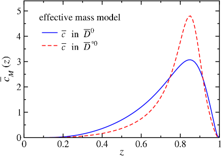
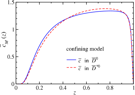
Figure 12: Anticharm quark distributions in charmed $D$ (solid) and $D^{*}$ (dashed) mesons, within the effective mass model (left), with the vertex form factor in Eqs. (76) and (77), and confining model (right), with the form factor in Eq. (78).

The results for the $\bar{c}$ distributions in the $D$ and $D^{*}$ mesons as computed formally in Eqs. (50 & 54) are illustrated in Fig. 12 for both types of vertex functions $G(\hat{s})$. In the absence of empirical constraints on PDFs in charmed mesons, the partonic cutoff $\hat{\Lambda}$ is a free parameter. However, since for heavy quarks the typical masses of the intermediate states ($DB$ or $\bar{c}q$) are comparable, to a first approximation we can fix $\hat{\Lambda}$ to the meson–baryon cutoff, $\hat{\Lambda}=\Lambda$. In the effective mass model, Eqs. (76) and (77), the peak of the anticharm distribution in $z$ reflects the fraction of the meson mass carried by the $\bar{c}$ quark. For both the $D$ and $D^{*}$ mesons, the $\bar{c}$ distribution peaks at $z\sim 0.85$, with the latter being slightly narrower. The distributions in the confining model, Eq. (78), also peak at similarly large momentum fractions, but are significantly broader.

A numerical feature of the effective mass model is the presence of the energy denominator $\propto(\hat{s}-m_{D}^{2})^{-2}$, which largely determines the qualitative shapes of the $\bar{c}$ distributions. For specific mass choices, $\hat{s}-m_{D}^{2}$ is minimized at a unique value of $z$, resulting in the strongly-peaked shapes observed in the effective mass model. In the confining model, on the other hand, the energy denominator responsible for this $z$ dependence is suppressed directly such that the resulting distribution shapes no longer possess pronounced maxima. In the effective charm model, however, the closer the energy denominator approaches its pole value, the more “singular” the behavior at the distribution maximum; as such, if we fix the charm and spectator masses according to Eq. (77), the energy denominator approaches the zero pole for heavier hadron masses, producing the more sharply peaked distributions seen in Fig. 12(a).

Charm in charmed baryons.

The calculation of the charm quark distributions in charmed baryons proceeds in similar fashion to that for the $D$ and $D^{*}$ mesons, but is more involved since the spectator system consists of two (or more) particles. In practice, however, one can simplify the calculation by treating the spectator $qq$ system as an effective “diquark” with a fixed mass $m_{qq}$. For spin-1/2 charmed baryons, in general the spectator diquark state can have either spin 0 or spin 1, with corresponding scalar and pseudovector vertex functions describing the momentum dependence. The spin of the spectator diquark can affect the spin and flavor dependence of the associated parton distribution; for example, the suppression of the $d/u$ ratio in the proton at large $x$ is usually attributed to a higher energy of the spin-1 diquark in the proton compared with the spin-0 diquark [178, 205]. Since here we are concerned with the total effect on the charm quark distribution, rather than the flavor dependence, it will be sufficient to consider only the leading contribution arising from the scalar spectators, for which we take an effective mass of $m_{qq}=1$ GeV.

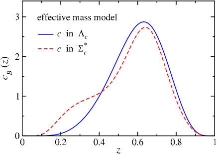
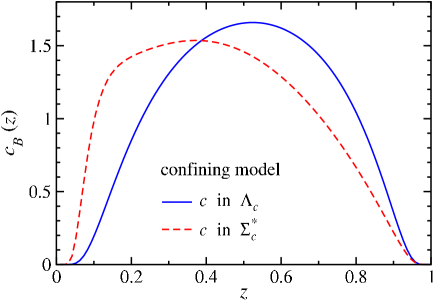
Figure 13: Charm distributions in the charmed $\Lambda_{c}$ (solid) and $\Sigma_{c}^{*}$ (dashed) baryons, within the effective mass model (left), and the confining model (right).

The resulting $c$ quark distributions in the spin-1/2 and spin-3/2 charmed baryons as generated by our formulas in Eqs. (58 & LABEL:eq:c_Sigma-st) are illustrated by Fig. 13; where relevant, we use the same numerical values for the masses and cutoffs as in the $\bar{c}$ calculation in the charmed mesons above. Compared with the $\bar{d}$ distributions in $D$ and $D^{*}$, the $c$ quark PDFs are peaked at somewhat smaller values of $z$. In the effective mass model for the $B$-$c$-$qq$ vertex function, both the $c$ distributions in $\Lambda_{c}$ and in $\Sigma_{c}^{*}$ are maximal at $z\approx 0.6-0.65$, with a relatively narrow distribution in $z$. The bulge in the $c$ distribution in the $\Sigma_{c}^{*}$ baryon is associated with the more complicated spin algebra compared with the $\Lambda_{c}$. The $c$ distributions with the confining model vertex function are once again somewhat broader, peaking at smaller $z$ values, $z\approx 0.55$ for the $\Lambda_{c}$ baryon and $z\approx 0.4$ for the $\Sigma_{c}^{*}$, with the latter having a sharp drop off at $z\to 0$. The broader distributions here are generated by the suppression of the energy denominator $(\hat{s}-M_{B}^{2})^{-2}$, which is mostly responsible for the strongly-peaked distributions in the effective mass model. In all cases the distributions have been normalized to respect the valence quark number sum rule, as in Eq. (60).

Having assembled the various ingredients for the calculation of the convolution expressions in Eqs. (9), in the next section we gather these inputs at last to compute the $c$ and $\bar{c}$ distributions in the nucleon.

3 Numerical results

Combining the distributions of $c$ and $\bar{c}$ quarks in the charmed mesons and baryons discussed in the previous section with the splitting functions summarized in Sec. 1, we present the resulting $c$ and $\bar{c}$ distributions in the physical nucleon. We consider in Sec. 1 contributions to the intrinsic charm PDFs $c(x)$ and $\bar{c}(x)$ from the various meson–baryon configurations in the MBM, as well as the dependence of the results on the models for the charm distributions inside the charm hadrons. To better control the systematic uncertainties within the calculation, we also compare our results with other prescriptions for intrinsic charm distributions in Sec. 2, and conclude the section with comparisons relative to measurements of the charm structure function $F^{c}_{2}$.

1 Intrinsic charm in the MBM

The contributions to the charm and anticharm quark distributions in the nucleon from various meson–baryon states are presented in Fig. 14, using as benchmark the confining model for the PDFs in the charmed hadrons (78) with a mass parameter $\Lambda=3$ GeV. The contributions correspond to the same configurations as in Fig. 10, namely, the dominant $\bar{D}^{*0}\Lambda_{c}^{+}$ state, the $\bar{D}^{0}\Lambda_{c}^{+}$ and $\bar{D}^{*0}\Sigma_{c}^{*+}$ states, as well as the (negligible) $\bar{D}^{0}\Sigma_{c}^{*+}$ contribution. As expected from the magnitudes of the splitting functions in Fig. 10, the $\bar{D}^{*}\Lambda_{c}^{+}$ state produces the dominant meson–baryon contribution.

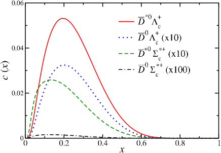
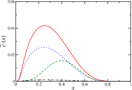
Figure 14: Charm (left) and anticharm (right) quark distributions in the nucleon in the MBM, with contributions from the meson–baryon configurations as in Fig. 10: $\bar{D}^{*0}\Lambda_{c}^{+}$ (red solid), $\bar{D}^{0}\Lambda_{c}^{+}$ (scaled $\times 10$, blue dotted), $\bar{D}^{*0}\Sigma_{c}^{*+}$ (scaled $\times 10$, green dashed), and $\bar{D}^{0}\Sigma_{c}^{*+}$ (scaled $\times 100$, black dot-dashed).

Summing over all the contributions listed in Fig. 8, the total $xc$ and $x\bar{c}$ distributions are shown in the left panel of Fig. 15, at the input scale $Q^{2}=m_{c}^{2}$ and evolved to $Q^{2}=50$ GeV² (which is typical for charm structure function measurements). In both cases, the dominant $\bar{D}^{*0}\Lambda_{c}^{+}$ contribution consistently accounts for approximately 70% of the total. An additional characteristic feature of our MBM evident in the left-hand side of Fig. 15 is the relative “hardness” of the $x\bar{c}(x)$ distribution over $xc(x)$ — a property that holds for every meson–baryon configuration in the MBM, reflecting the fact that the charm quark represents a larger fraction of the total mass of the meson than of the baryon. Since the peak in the charm distribution in a hadron is related to the fraction of the hadron mass carried by the charm quark, the resulting distribution of $\bar{c}$ in the $\bar{D}$ meson will typically be harder than that for the $c$ in the $\Lambda_{c}$. While it is possible to make the intrinsic $c$ distribution as hard as the $\bar{c}$ distribution in convolution models, doing so generally requires rather unnatural parton distributions inside the baryon and meson states.

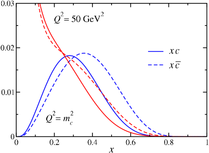
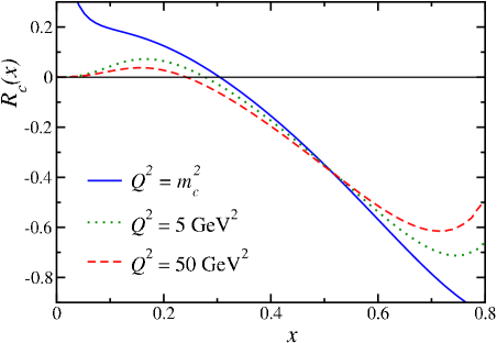
Figure 15: (Left) Total $xc$ (solid lines) and $x\bar{c}$ (dashed lines) distributions in the MBM with the confining model for the PDFs in the charmed hadrons, Eq. (78), at $Q^{2}=m_{c}^{2}$ (blue) and evolved to $Q^{2}=50$ GeV² (red). (Right) Corresponding charm–anticharm asymmetry $R_{c}(x)=(c(x)-\bar{c}(x))/(c(x)+\bar{c}(x))$ at $Q^{2}=m_{c}^{2}$ (solid), $Q^{2}=5$ GeV² (dotted), and $Q^{2}=50$ GeV² (dashed).

To quantify the magnitude of the nonperturbative charm in the nucleon, we can compute the total proton momentum carried by charm and anticharm quarks,

$$P_{c} = C^{(1)}+\overline{C}^{(1)}\ ,$$ (79)

where the moments $C^{(1)}$ and $\overline{C}^{(1)}$ are defined in Eqs. (12). For the confining model distributions in the charmed mesons and baryons, the momentum fraction at the input model scale $Q^{2}=m^{2}_{c}$ is found to be $P_{c}=1.34^{\,+1.35}_{\,-0.75}\,\%$ for the cutoff mass parameter $\Lambda=(3.0\pm 0.2)$ GeV obtained from the inclusive $\Lambda_{c}$ production data, Sec. 1. Again we note that these first moments differ numerically from the charm multiplicities also mentioned in Sec. 1, where we found $\langle n\rangle_{MB}^{\rm(charm)}=2.40^{\,+2.47}_{\,-1.36}\,\%$. The strong dependence of the total momentum on $\Lambda$ stems from the controlling influence of the dominant meson–baryon splitting function on the hadronic form factor, as seen in the left panel of Fig. 11. Contrastingly, the BHPS model normalized to a 1% charm probability in the nucleon yields a corresponding momentum fraction of $P_{c}=0.57$%; our MBM at $\Lambda=3$ GeV therefore predicts about twice the intrinsic charm momentum as the BHPS model.

Valence quark normalization requires that the first moment of $c-\bar{c}$ vanishes, as in Eq. (16), which follows for any splitting function that obeys the reciprocity relation, Eq. (11). Higher moments, on the other hand, are not required to vanish. In fact, the magnitude of the $c-\bar{c}$ asymmetry can be quantified in terms of the difference of the second moments (momentum carried by charm and anticharm quarks),

$$\Delta P_{c} = C^{(1)}-\overline{C}^{(1)}\ .$$ (80)

At the model scale $Q^{2}=m_{c}^{2}$, we find $\Delta P_{c}=-(0.13^{\,+0.14}_{\,-0.08})\,\%$ for $\Lambda=(3.0\pm 0.2)$ GeV. The overall negative values of $\Delta P_{c}$ follow from the behavior in the MBM that the $\bar{c}$ distribution is harder than the $c$ as we just argued.

The momentum imbalance of anticharm quarks compared to charm can be estimated from the ratio of the difference $\Delta P_{c}$ to the sum $P_{c}$, for which we find $\Delta P_{c}/P_{c}\approx-10\%$. As a function of $x$, however, the imbalance is not uniformly distributed. Defining the ratio

$$R_{c}(x) = \Big{(}c(x)-\bar{c}(x)\Big{)}\Big{/}\Big{(}c(x)+\bar{c}(x)\Big{)}\ ,$$ (81)

we see from the RHS of Fig. 15 that the relative asymmetry can exceed 50% at large values of $x$ ($x\gtrsim 0.5$). The $Q^{2}$ dependence of the ratio indicates relatively mild effects over the large range considered (up to $Q^{2}=50$ GeV²), with the slope of the asymmetry becoming slightly more shallow with increasing $Q^{2}$. Note that the ratio $R_{c}$ is nonzero at $x=0$ at the model scale, but perturbative evolution forces $R_{c}(x=0)$ to vanish at large $Q^{2}$ due to the growth of the denominator $c+\bar{c}$.

2 Comparison with other models

While some of the features of the nonperturbative $c$ and $\bar{c}$ distributions in the MBM are relatively robust, such as the generally harder $x$ dependence compared with the perturbatively generated distributions and the presence of a $c-\bar{c}$ asymmetry, the detailed $x$ dependence does depend on the specifics of the model.

To estimate the model dependence of the calculated $c$ and $\bar{c}$ PDFs, we compare the results obtained in the previous section, using the splitting functions and quark distributions from Sec. 2 and the confining prescription for the PDFs in the charmed hadrons of Sec. 2, with distributions computed under various assumptions and approximations.

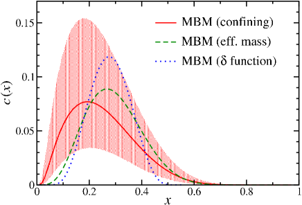
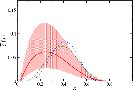
Figure 16: Model dependence of the charm distributions in the nucleon for $c(x)$ (left) and $\bar{c}(x)$ (right), for the MBM with the confining model for the PDFs in charmed hadrons (red solid), the effective mass model (green dashed), and the $\delta$ function model (blue dotted). All distributions use a common value for the cutoff mass of $\Lambda=(3.0\pm 0.2)$ GeV, with the uncertainty band shown for the confining model.

Within the same MBM framework, if one instead uses the effective mass model as defined in Eq. (77) for the (anti-)charm distributions in intermediate states, the resulting $c$ and $\bar{c}$ distributions in the nucleon are slightly harder, especially for the $\bar{c}$, as Fig. 16 illustrates. This generally follows from the shape of the $\bar{c}_{M}$ distribution in the confining and effective mass models in Fig. 12, where the latter is more strongly peaked at large values of the parton momentum fraction.

The corresponding value of the total nucleon momentum carried by charm and anticharm quarks in the effective mass model is $P_{c}=1.67^{\,+1.70}_{\,-0.94}\,\%$ for cutoff masses $\Lambda=(3.0\pm 0.2)$ GeV, and $\Delta P_{c}=-(0.24^{\,+0.28}_{\,-0.14})\,\%$ for the momentum asymmetry, with the resulting momentum imbalance $\Delta P_{c}/P_{c}\approx-15\%$. The $c-\bar{c}$ asymmetry in this model is therefore more pronounced than in the confining model.

In a more simplified approach, the $c$ and $\bar{c}$ distributions inside the charmed hadrons were approximated in Ref. [178] by $\delta$ functions centered at the $x$ values corresponding to the fraction of the hadron mass carried by the constituent charm or anticharm quark,

$$c_{B}(x)=\delta(x-x_{B})\hskip 8.5359pt{\rm and}\hskip 8.5359pt\overline{c}_{M}(x)=\delta(x-x_{M}).$$ (82)

From Eqs. (9), the charm and anticharm distributions in the nucleon are then given directly as sums over the various meson–baryon splitting functions,

$$c(x) = \sum_{B,M}\,\frac{1}{x_{B}}\,f_{BM}\left(\frac{x}{x_{B}}\right)\ ,$$ (83a)

$$\bar{c}(x) = \sum_{M,B}\,\frac{1}{x_{M}}\,f_{MB}\left(\frac{x}{x_{M}}\right)\ .$$ (83b)

This is especially easy to see if we use an equivalent form for the relevant convolution in Eqs. (9); for instance for anticharm:

$$\bar{c}(x)\ =\ \sum_{M,B}\ \int dx_{1}\int dx_{2}\ f_{MB}(x_{1})\ \bar{c}_{M}(x_{2})\ \delta(x-x_{1}x_{2})$$

$$=\ \sum_{M,B}\ \int_{0}^{1}{dx_{2}\over x_{2}}\ f_{MB}\left({x\over x_{1}}\right)\delta(x_{2}-x_{M})\ ,$$ (84)

whence comes the expression for $\bar{c}(x)$ in Eq. (83).

Since the masses of the charm quark [$m_{c}={\cal O}(1.5~{}{\rm GeV})$] and the $D$ mesons [$m_{D}={\cal O}(\mbox{1.8--2}~{}{\rm GeV})$] are similar, as a first approximation one can take $x_{M}\approx 1$. Similarly, for the fractional mass of the $c$ quark in the charmed baryon, the approximation $x_{B}\approx 2/3$ was utilized [178]. In a somewhat more sophisticated approach, one can choose $x_{M}$ and $x_{B}$ to minimize the $\hat{s}$-dependent energy denominator, which depends on the combination $m_{c}^{2}/x+m_{\rm spec}^{2}/(1-x)$, where the spectator mass $m_{\rm spec}$ corresponds to the light quark mass $m_{u,d}$ for a meson, and to an effective diquark mass $m_{qq}$ for a baryon. Choosing $m_{c}=1.3$ GeV, $m_{u,d}=0.313$ GeV and $m_{qq}=1$ GeV, one has

$$x_{B}\,=\,\frac{m_{c}}{m_{c}+m_{qq}}\approx 0.57\ ,\ \ \ \ \ \ x_{M}\,=\,\frac{m_{\bar{c}}}{m_{\bar{c}}+m_{u,d}}\approx 0.81\ .$$ (85)

For the best fit form factor cutoff mass $\Lambda=3$ GeV, the momentum carried by charm in this $\delta$ function approximation model is $P_{c}=1.66$%, which is slightly greater than in the MBM confining or effective mass models.

In Fig. 16 we compare the $c$ and $\bar{c}$ distributions in the MBM obtained using the confining model PDFs in the charmed hadrons with those computed from the effective mass model and $\delta$ function approximations, with a common cutoff mass $\Lambda=(3.0\pm 0.2)$ GeV. The MBM confining model distributions are generally softer than those in the effective mass and $\delta$ function schemes, with the confining model giving a slightly broader shape, and the $\delta$ function model having the narrowest distribution. Within the uncertainty bands of the parameters (for clarity we have only shown the uncertainty band for the confining model in Fig. 16), the distributions are indeed compatible with each other. In all three models the anticharm distributions are clearly harder than the charm, so that the qualitative features of the ratio $R_{c}$ in Fig. 15 are largely retained. Interestingly, the $\delta$ function model gives an $x$ dependence for the charm PDFs that closely resembled the shape of the effective mass model distributions for $\Lambda=3$ GeV. This feature may be exploited in simplified calculations that aim simply to approximate general features of nonperturbative charm distributions.

The charm structure function $F^{c}_{2}$.

Having explored the model dependence of the total intrinsic $c$ and $\bar{c}$ distributions in the nucleon, we can now directly confront the results with measurements of the charm structure function, $F_{2}^{c}$. This will provide additional constraints on the model parameters, complementing those of the inclusive $\Lambda_{c}$ production in $pp$ scattering discussed in Sec. 1.

Thought the calculations of intrinsic charm in this analysis have been normalized to inclusive charm production data in $pp$ collisions as discussed in Sec. 1, the results may also be confronted with data on the charm structure function $F_{2}^{c}$ obtained from measurements of charm production cross sections in deep-inelastic lepton scattering. In comparing with experimental measurements of $F_{2}^{c}$, in addition to intrinsic charm arising from nonperturbative fluctuations of the nucleon into states with 5 or more quarks, one must also consider the “extrinsic” charm arising from gluon radiation to $c\bar{c}$ pairs, which is described by perturbative QCD evolution. As we have already seen in the discussion of high-$Q^{2}$ CSV, these effects at LO in $\alpha_{s}$ are embodied by the diagrams in Fig. 13 and Eqs. (62).

To lowest order in the strong coupling constant $\alpha_{s}$, the charm structure function is straightforwardly related to the $c$ and $\bar{c}$ parton distributions in the nucleon,

$$F_{2}^{c}(x,Q^{2})=\frac{4x}{9}\left[c(x,Q^{2})+\bar{c}(x,Q^{2})\right]\ .$$ (86)

When combining the two charm contributions, it is necessary to assign a scale $Q_{0}^{2}$ at which the nonperturbative charm is generated, and then evolve this to the relevant $Q^{2}$ for comparison with experiment. While the absolute scale of the intrinsic contribution is a characteristic ingredient of the model (in our case, the MBM), it is customary to set this to the effective charm quark mass, $Q_{0}^{2}=m_{c}^{2}=1.69$ GeV².

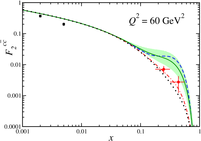
Figure 17: Charm structure function $F_{2}^{c}$ at 60 GeV². The perturbative QCD calculation (black dotted line) is compared with nonperturbative charm contributions in the MBM using the confining model with cutoff $\Lambda=(3.0\pm 0.2)$ GeV (green solid line and shaded band), confining model with $\Lambda=2.5$ GeV (red dot-dashed line), and effective mass model with $\Lambda=3.0$ GeV (blue dashed line). The data are from H1 and ZEUS (black squares) and EMC (red circles).

The calculated charm structure function $F_{2}^{c}(x,Q^{2})$ is shown in Fig. 17 at $Q^{2}=60$ GeV², and compared with data from the H1 [184] and ZEUS [185] Collaborations at HERA and with higher-$x$ data from EMC [183]. While the extrinsic charm distribution is generated completely perturbatively by evolving an initial “zero distribution” $c(x,Q^{2}_{0})=\bar{c}(x,Q^{2}_{0})\equiv 0$ with the next-to-leading order evolution code from Ref. [206], nonperturbative models for $F_{2}^{c}$ of course start with the MBM predictions at the scale $Q_{0}^{2}$ as just described. Since the experimental $Q^{2}$ values are large compared to $m_{c}^{2}$, standard massless QCD evolution in the form of the Variable Flavor Number Scheme is appropriate.

As has been suggested previously [215], at $Q^{2}=60$ GeV² the perturbative results usually underestimate the EMC data at high $x$, and the addition of a nonperturbative contribution raises the total $F_{2}^{c}$ in rough proportion to the amount of intrinsic charm assumed in the model. However, for our MBM with the confining model vertex functions, $\Lambda=(3.0\pm 0.2)$ GeV generally leads to overestimation of the EMC $F_{2}^{c}$ data at large $x$ and high $Q^{2}$, being marginally consistent with the data at the lower edge of the error band. Using instead the MBM with the effective mass model vertex functions and the same cutoff $\Lambda=3.0$ GeV, the peak at large $x$ is still more pronounced, and hence overestimates the EMC data to a slightly greater extent. Lowering the cutoff to $\Lambda=2.5$ GeV for the confining model, the resulting $F_{2}^{c}$ is in better agreement with the data, producing a smaller overestimate of the lower-$Q^{2}$ data points and resulting in a better fit to the $Q^{2}=60$ GeV² data. Note that for such a small cutoff the average charm normalization $\langle n\rangle_{MB}^{\rm(charm)}\lesssim 0.5\%$, which would significantly underestimate the inclusive $\Lambda_{c}^{+}$ production data (see Fig. 9).

4 A Global Analysis of IC

Having constructed a systematic framework for the analysis of intrinsic charm in Secs. 1–3, we turn now to a more comprehensive effort [176] to constrain its overall normalization via QCD global analysis. There have in fact already been several attempts of this sort.

In an earlier study [181], Pumplin, Lai and Tung carried out a global fit to high-energy data with phenomenological PDFs including an intrinsic charm component at the starting scale $Q_{0}=m_{c}$. Using several different phenomenological forms for the intrinsic charm (including the BHPS model, Eq. (3), a scalar MBM employing Eq. (4), and a “sea-like” charm model), the magnitude of the charm contribution was varied until a substantial increase in the $\chi^{2}$ was found with the set of global high-energy data. The analysis found that the global fits could accommodate charm momentum fractions of $P_{c}\approx 2\%$ in the BHPS and scalar MBM models and $P_{c}\approx 2.5\%$ in the sea-like model at the 90% confidence level, which are significantly larger than the constraints from the EMC $F_{2}^{c}$ data, and at the upper boundary of the range allowed by the ISR R608 $\Lambda_{c}^{+}$ production data. The more recent update [182] that includes NNLO corrections finds $P_{c}\leq 1.5\%$ for the sea-like model and $P_{c}\leq 2.5\%$ for the BHPS model at the scale $Q_{0}$.

We should note, however, that while the analysis in Ref. [181] fitted the precision low-$x$ charm structure function data from H1 and ZEUS, it did not include the EMC $F_{2}^{c}$ data at large $x$ [219], which results in tighter constraints on the magnitude of the intrinsic charm as we now show by explicit computation. Moreover, while the very same EMC data are occasionally mentioned [215] as a leading evidence for intrinsic charm, they have never been incorporated systematically into an analysis such as the present one.

Like these previous studies, e.g., [181, 182], we find it most natural to fit the total momentum carried by the nonperturbative $c(x),\ \bar{c}(x)$ contained in five-quark Fock states latent in the foregoing meson-baryon model. Explicitly, this is

$$\langle x\rangle_{\rm IC}\equiv\int_{0}^{1}dx\,x\,[c(x)+\bar{c}(x)]\ .$$ (87)

We saw that the distribution shapes can be reasonably well-determined by the relativistic wavefunctions employed to describe contributions from the $SU(4)$ spectrum shown in Fig. 8 (after fitting the momentum cutoff $\Lambda$ to the $pp\rightarrow\Lambda_{c}X$ data of Fig. 9); this procedure imposes $\Lambda=(3.0\pm 0.2)$ GeV, but perhaps less clearly limits the overall normalization of IC in the proton as evidenced by the sizable uncertainty extracted in Sec. 1 for the relevant moments:

$$\langle n\rangle_{MB}^{\rm(charm)}=2.40^{\,+2.47}_{\,-1.36}\,\%\ ,\hskip 42.67912ptP_{c}=1.34^{\,+1.35}_{\,-0.75}\,\%\ .$$ (88)

That being the case, it is useful to extend the analysis of preceding sections by considering the world’s $F_{2}^{c}$ and other high-energy scattering data, and performing a new global QCD analysis along the lines of the recent JR14 fit [214]. Unlike the previous global analyses [181, 182] which placed more stringent cuts on the data ($Q^{2}\gtrsim 4$ GeV² and $W^{2}\gtrsim 12$ GeV²), excluding, for instance, all fixed target cross section measurements from SLAC [123], we include all available data sets with $Q^{2}\geq 1$ GeV² and $W^{2}\geq 3.5$ GeV².

In order to have simple analytic forms to serve the QCD fit of the IC normalization, we follow Ref. [180] and provide compact three-parameter fits to the $c$ and $\bar{c}$ PDFs in the MBM computed using several different models for the charm quark distributions in the charmed mesons and baryons, including the confining model, effective mass model, and the $\delta$ function model. The parameters matching the best fits to each of these models generated at $\Lambda=3$ GeV are then given in Table 3. The parametric form for the charm distributions in the nucleon for the confining and effective mass models is taken to be

$$c(x) = C^{(0)}\,A\,x^{\alpha}(1-x)^{\beta}\ ,$$ (89a)

$$\bar{c}(x) = C^{(0)}\,\bar{A}\,x^{\bar{\alpha}}(1-x)^{\bar{\beta}}\ ,$$ (89b)

where the normalization constants $A=1/B(\alpha+1,\beta+1)$ and $\bar{A}=1/B(\bar{\alpha}+1,\bar{\beta}+1)$, with $B$ the Euler beta function, ensure that the distributions are normalized to $C^{(0)}$.

Table 3: Best fit parameter values for the $c$ and $\bar{c}$ distributions in the nucleon in Eqs. (89) and (90) in the MBM for a central cutoff mass $\Lambda=3.0$ GeV.

$c$, $\bar{c}$ fit	confining	effective	$\delta$ function
parameters	model	mass model	model
$A$	$1.720\times 10^{2}$	$1.052\times 10^{2}$	$2.638\times 10^{5}$
$\alpha$	1.590	3.673	4.266
$\beta$	6.586	10.16	4.485
$\bar{A}$	$7.404\times 10^{1}$	$4.160\times 10^{0}$	$2.463\times 10^{4}$
$\bar{\alpha}$	1.479	4.153	5.003
$\bar{\beta}$	4.624	6.800	4.857

For the $\delta$ function model, where the $c$ and $\bar{c}$ PDFs in the charmed hadrons are given by $\delta$ functions in $x$, it is more convenient to parametrize the distributions in Eqs. (83) as

$$c(x) = C^{(0)}\,A\,x^{\alpha}(x_{B}-x)^{\beta}\,\theta(x_{B}-x)\ ,$$ (90a)

$$\bar{c}(x) = C^{(0)}\,\bar{A}\,x^{\bar{\alpha}}(x_{M}-x)^{\bar{\beta}}\,\theta(x_{M}-x)\ ,$$ (90b)

with $x_{B}$ and $x_{M}$ given by Eq. (85). Note that in each of these prescriptions, it is simple to use Eq. (87) to go between the specific $C^{(0)}$ preferred by fits and the values of $\langle x\rangle_{\rm IC}$ plotted in subsequent figures.

The guiding philosophy of QCD global analysis [211] is the validity of the factorization theorem, which posits the separability of QCD-mediated processes into hard and soft components. For instance, in the case of the electromagnetic structure functions of a hadron $h$,

$$F^{\gamma}_{ih}(x,Q^{2})\ =\ \sum_{f}\ \int_{0}^{1}\ {d\xi\over\xi}\ C^{\gamma f}_{i}\left({x\over\xi},{Q^{2}\over\mu^{2}},{\mu^{2}_{F}\over\mu},\alpha_{S}(\mu^{2})\right)\ \cdot\ \phi_{f/h}(\xi,\mu^{2}_{F},\mu^{2})\ ,$$ (91)

suggests that the $F^{\gamma}_{ih}(x,Q^{2})$ contain information on the universal parton densities$\phi_{f/h}(\xi,\mu^{2}_{F},\mu^{2})$ of flavor $f$; these in turn may be found with high precision given an accurate computation of the hard process encoded in the coefficient function $C^{\gamma f}_{i}$. The presence of the renormalization and factorization scales $\mu,\ \mu_{F}$ demands that we must elect to use a particular scheme, upon which our results will depend. In the present treatment we consistently compute in the $\overline{\rm MS}$ scheme.

For the QCD analysis we use the framework of the JR14 global analysis [214], in which the total $F_{2}$ structure function is given by

$$F_{2}=F_{2}^{\rm light}+F_{2}^{\rm heavy}\ ,$$ (92)

where $F_{2}^{\rm light}$ denotes the light-quark ($u$, $d$, $s$) contributions, and $F_{2}^{\rm heavy}$ includes contributions from the heavy $c$ and $b$ quarks. The charm structure function is further decomposed into a perturbative part, $F_{2}^{c\bar{c}}$, and a nonperturbative (IC) component, $F_{2}^{\rm IC}$,

$$F_{2}^{c}=F_{2}^{c\bar{c}}+F_{2}^{{}^{\rm IC}}\ .$$ (93)

The perturbative contribution is computed in the fixed-flavor number scheme (FFNS) from the photon-gluon fusion process,

$$F_{2}^{c\bar{c}}(x,Q^{2},m_{c}^{2})=\frac{Q^{2}\alpha_{s}}{4\pi^{2}m_{c}^{2}}\sum_{i}\int\frac{dz}{z}\ \hat{\sigma}_{i}(\eta,\xi)\ \cdot\ f_{i}\Big{(}\frac{x}{z},\mu\Big{)}\ ,$$ (94)

where $\hat{\sigma}_{i}$ is the hard scattering cross section for the production of a $c\bar{c}$ pair from a parton of flavor $i$, with $i=u,d,s$ or $g$, and $f_{i}$ is the corresponding parton distribution, both calculated to NLO [${\cal O}(\alpha_{s})$] accuracy. The partonic cross section $\hat{\sigma}_{i}$ is evaluated as a function of the variables $\xi=Q^{2}/m_{c}^{2}$ and $\eta=Q^{2}\cdot(1-z)\big{/}(4m^{2}_{c}z)-1$; the PDF is computed at the factorization scale $\mu_{F}^{2}=4m_{c}^{2}+Q^{2}$, where the charm mass is $m_{c}=1.3$ GeV at threshold.

On the other hand, $F_{2}^{{}^{\rm IC}}$ of Eq. (93) is actually specified only at the charm production threshold by the MBM of the previous sections; whereas before we relied upon a brute-force integration of the DGLAP equations to render Eq. (86) at the $Q^{2}$ of the EMC measurements, we now require a more thorough scheme to complement the photon-gluon FFNS used in Eq. (94). For this purpose, we turn to the ansätz of Hoffmann and Moore described in [212].

In this method, the scale dependence of the IC distributions parametrized in Eqs. (89) is incorporated through target and quark mass effects as implemented in the OPE — much as described in Sec. 1. A version of Eq. (11), slightly altered to depend on the heavy quark mass, therefore rescales the intrinsic distributions as

$$c(x)\ \,\,\,\,\rightarrow\,\,\,\,c(\xi_{c},\gamma_{c})\ =\ c(\xi_{c})-{\xi_{c}\over\gamma_{c}}\ c(\gamma_{c})\ \iff\ \xi_{c}<\gamma_{c}$$ (95)

$$=0\ \iff\ \xi_{c}\geq\gamma_{c}\ ,$$ (96)

where the modified Nachtmann variable is now

$$\xi_{c}\ =\ {2ax\over\left(1+\sqrt{1+4x^{2}M^{2}\Big{/}Q^{2}}\right)}\ ,\hskip 42.67912pta={1\over 2}\ \Big{(}1+\sqrt{1+4m^{2}_{c}\Big{/}Q^{2}}\Big{)}\ .$$ (97)

$\gamma_{c}$ serves as another means of circumventing the OPE threshold problem, in this case by simply terminating input distributions at $\xi_{c}<\gamma_{c}$, where the latter is just $\xi_{c}$ evaluated at $x=\hat{x}\mathrel{\vbox{\hbox{\scriptsize.}\hbox{\scriptsize.}}}=Q^{2}\Big{/}(Q^{2}+4m^{2}_{c}+M^{2})$.

With these expressions, we can write the full OPE result:

$$F_{2}^{{}^{\rm IC}}\ =\ {4x^{2}\over 9(1+4x^{2}M^{2}/Q^{2})^{3/2}}\ \left\{{1+4m^{2}_{c}/Q^{2}\over\xi_{c}}\ \Big{(}c(\xi_{c},\gamma_{c})+\bar{c}(\xi_{c},\gamma_{c})\Big{)}\ +\ 3\hat{g}(\xi_{c},\gamma_{c})\right\}\ ,$$ (98)

$$\hat{g}(\xi_{c},\gamma_{c})\ =\ {2xM^{2}/Q^{2}\over(1+4x^{2}M^{2}/Q^{2})}\ \int_{\xi_{c}}^{\gamma_{c}}\ {dt\over t}\ \left(c(t,\gamma_{c})+\bar{c}(t,\gamma_{c})\right)\$$ (99)

$$\hskip 128.0374pt\times\left[1+2xtM^{2}/Q^{2}+2xM^{2}/(tQ^{2})\right]\cdot\left(1-{m^{2}_{c}\over t^{2}M^{2}}\right)\ .$$

The expression in Eq. (98), together with NLO corrections from gluon loops and bremsstrahlung, is the primary input to the global analysis by which we constrain $\langle x\rangle_{\rm IC}$. For a detailed description of the choice of data and kinematic cuts we refer to the JR14 analysis; however, whenever possible the original cross section data were used rather than structure functions and ratios of structure functions extracted from those cross sections. Since data at relatively low $Q^{2}$ were used in this global fit, higher-twist corrections were employed for the low-$Q^{2}$ data. For deuteron data nuclear corrections were supplied by the CJ group [216], while for data on heavier nuclei nuclear corrections were used from nDS09 [217].

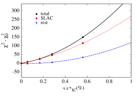
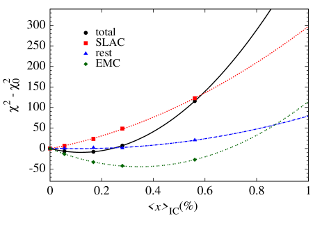
Figure 18: Contributions of various data sets to $\chi^{2}$ vs. $\langle x\rangle_{\rm IC}$. Solid circles: total $\chi^{2}$; red squares: contribution from SLAC data [213]; blue triangles: all other data sets. EMC $F^{c}_{2}$ data is excluded in the left panel. The right panel includes EMC charm data, and the resulting contribution to $\chi^{2}$ is represented by open green squares.

Our results for intrinsic charm are summarized in Fig. 18, where the solid circles show the total $\chi^{2}$ for the global fit vs. the fraction of the proton momentum carried by intrinsic charm. The left panel shows the result excluding the EMC inclusive charm leptoproduction data, while the lower panel includes EMC charm data. Results were calculated using the confining approximation of Table 3 as a proxy for the other models, which yield qualitatively similar constraints to $\langle x\rangle_{\rm IC}$. The upper limit allowed for momentum carried by charm quarks is a fraction of a percent; namely, the $\chi^{2}$ profile for the ‘Total’ fit without EMC $F_{2}^{c\bar{c}}$ data in the top panel of Fig. 18 excludes an IC of $\langle x\rangle_{\rm IC}\geq 0.1$ at the $5\sigma$ level. This high level of exclusion is largely due to the constraints provided by SLAC data [213]. In the absence of the SLAC data – that is, for the ‘Rest’ fits shown as blue dot-dashed lines in Fig. 18 – results are comparable to earlier CTEQ findings [181] when statistical tolerances are considered. Namely, $\langle x\rangle_{\rm IC}=0.1\%$ is contained within the $1\sigma$ interval. On the other hand, the $2\sigma$ and $3\sigma$ confidence levels permit IC up to $\langle x\rangle_{\rm IC}=0.2\%$ and $0.3\%$, respectively. If the $\Delta\chi^{2}=100$ statistical tolerance of CTEQ is used, these limits must be multiplied by $10$ to give, for instance, $\langle x\rangle_{\rm IC}=2.0\%$ at the $2\sigma$ C.L., in agreement with [181].

Thus, if the EMC data are to be neglected, the minimum of the $\chi^{2}$ curve occurs at $\langle x\rangle_{\rm IC}=0$. On the contrary, including EMC data gives a best value $\langle x\rangle_{\rm IC}=0.13\pm 0.04$%, also at the $1\sigma$ level. Clearly this is a much smaller upper limit on IC than obtained by the CTEQ analysis from Dulat et al. [182], who found that their global analysis allowed IC momentum up to 2.5%.

This sharp discrepancy is understandable in light of the content of Fig. 18. The red squares show the contribution to $\chi^{2}$ from SLAC $ep$ and $ed$ data [213], while the blue triangles show the contribution from all the remaining data. The rapid take-off of the red curves highlights the fact that the limits on intrinsic charm are dominated by the SLAC DIS data — especially those at low-$Q^{2}$ and high-$x$. But this is of course precisely the kinematic regime at which one would anticipate the effects of nonperturbative heavy quarks to be most sizable. Contrastingly, the kinematic cuts of the CTEQ and MSTW global fits [218, 120] are targeted at high energy collider processes typified by the LHC, and consequently emphasize data at substantially lower $x$ and higher $Q^{2}$.

The global fits, either with or without the EMC charm data, agree very well with the inclusive charm electroproduction measurements at HERA [220]; our results are essentially identical with those given in Fig. 10 of the JR14 analysis [214]. The HERA data are at very small $x$, a region where intrinsic charm is relatively unimportant. On the other hand, the global fits here do poorly in reproducing the EMC inclusive charm data, as evidenced by the fact that the fit quality degrades sharply to $\chi^{2}/\mathrm{d.o.f.}=4.3$ for those measurements. In fact, regardless of whether the fits are or are not directly constrained by the EMC charm data, they are not well fit — a finding which suggests that the EMC points, being older and considerably less precise than the HERA data, have significant tension with the latter. This fact necessarily calls into question the reliability of such data for the purposes of extracting a nonperturbative component of $F^{c}_{2}$ at higher $x$.

Chapter 5 Epilogue: The pion cloud and final state tagging

“Almost everybody that’s well-known gets tagged with a nickname.”
      — Alan Alda

In spite of its early discovery [221] and numerous decades of related phenomenology, much remains unknown regarding the structure and interactions of the pion. Nowhere is this quite as evident as in the still-perplexing behavior of the pion electromagnetic form factor $F_{\pi}(Q^{2})$, which is traditionally accessed via exclusive processes such as electroproduction and defined as

$$q^{2}<0\ \implies\ \langle\pi^{+}(k^{\prime})|J_{\mu}(0)|\pi^{+}(k)\rangle\ =\ e(k_{\mu}+k^{\prime}_{\mu})\ F_{\pi}(q^{2})\ ,$$ (1a)

$$q^{2}>0\ \implies\ \langle\pi^{+}(k^{\prime})\pi^{-}(k)|J_{\mu}(0)|0\rangle\ =\ e(k^{\prime}_{\mu}-k_{\mu})\ F_{\pi}(q^{2})\ ,$$ (1b)

where as usual, $Q^{2}=-q^{2}$, the 4-momenta are $q=k^{\prime}-k$ in Eq. (1a), and $q=k+k^{\prime}$ in Eq. (1b), and a normalization condition ensures $F_{\pi}(0)=1$. For spacelike $Q^{2}>0$, $F_{\pi}(Q^{2})$ is indeed calculable in the context of pQCD [222], which suggests a very simple form for its asymptotic behavior; namely,

$$Q^{2}\gg\Lambda^{2}_{QCD}\,\,\,\,\,:\ \,\,\,\,Q^{2}F_{\pi}(Q^{2})\ \sim\ 16\pi\ \alpha_{s}(Q^{2})\ f^{2}_{\pi}\omega^{2}_{\pi}\ ,$$ (2)

in which the pion decay constant is $f_{\pi}=93$ MeV, and $\omega_{\pi}$ depends upon the behavior of the valence parton distribution amplitude of the pion, and approaches unity at sufficiently large $Q^{2}$.

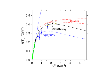
Figure 1: (Left) As illustrated in this plot from [223], the behavior of the spacelike pion form factor has been the object of many modeling efforts, given the ambiguity of the $Q^{2}$ scale at which the pQCD result of Eq. (2) becomes an accurate description. (Right) As we shall demonstrate, the pion cloud of the nucleon is responsible for potential flavor asymmetries in the light quark sea as computed in [224].

Of course there has been no shortage of experimental determinations of $F_{\pi}(Q^{2})$ as shown, for instance, in the left panel of Fig. 1, but these have typically been at rather shallow values of $Q^{2}$, and therefore not adequately near the expected transition region at which the onset of the pQCD prediction of Eq. (2) should begin. Rather, at these intermediate kinematics ($2\lesssim Q^{2}\lesssim 5$ GeV²) there exists a menu of discrepant model predictions that necessitate various proposed and upcoming measurements [225]. Typically, these measurements seek to access the $F_{\pi}(Q^{2})$ form factor at intermediate $Q^{2}$ via extrapolation to a physical $t=m^{2}_{\pi}$ pole based upon pion electroproduction measurements off the proton obeying

$${d\sigma\over dt}\ \sim\ g^{2}_{\pi NN}\ \left[{-t\over(t-m^{2}_{\pi})^{2}}\right]\ Q^{2}F^{2}_{\pi}(Q^{2})\ ,$$ (3)

which results from a “pion cloud” picture of nucleon structure similar to what we present shortly.

Moreover, through the dynamics of the Sullivan process [226] as described in the preceding analysis of Chap. 4 for intrinsic charm, the pion is expected to contribute crucially to various nonperturbative aspects of the nucleon’s flavor and spin decomposition. In particular, the parton distributions in the nucleon are expected to receive contributions of the form

$$\delta q(x)\ =\ \Big{\{}\delta^{[\pi N]}q(x)\ +\ \delta^{[N\pi]}q(x)\Big{\}}\ +\ \dots\ ,$$ (4a)

$$\delta\bar{q}(x)\ =\ \Big{\{}\delta^{[\pi N]}\bar{q}(x)\ +\ \delta^{[N\pi]}\bar{q}(x)\Big{\}}\ +\ \dots\ .$$ (4b)

Among other things, the differing flavor content of the charge states in the isovector pion triplet implies that the combinations contained in Eq. (4) would naturally induce flavor asymmetries such as $\bar{d}/\bar{u}\neq 1$, plotted in the right panel of Fig. 1. In fact, it was the observation of strong violations of the Gottfried Sum Rule defined in Eq. (5b) by NMC [227] that called attention to the experimental significance of light quark asymmetries and gave added currency to modeling efforts aimed at nonperturbative effects in the nucleon quark sea. This is simple to see by unpacking the expression in Eq. (5b) using the QPM under the assumption of partonic charge symmetry (unlike the analyses of Chap. 2.3); using the electromagnetic quark-level expressions of Eq. (31), we get

$$S_{G}\ =\ \int\ {dx\over x}\ \Big{(}F^{p}_{2}(x,Q^{2})-F^{n}_{2}(x,Q^{2})\Big{)}$$

$$=\ \sum_{q}\ e^{2}_{q}\int dx\ \left\{q^{p}_{v}(x)+2\bar{q}^{p}(x)\ -\ \Big{(}q^{n}_{v}(x)+2\bar{q}^{n}(x)\Big{)}\right\}$$

$$={1\over 3}\ \left\{1\ +\ 2\int_{0}^{1}dx[\bar{u}(x)-\bar{d}(x)]\right\}\ ,$$ (5)

such that the original NMC finding $S_{G}=0.240\pm 0.016$ suggests an $SU(2)$ flavor symmetry breaking pattern that favors $\bar{d}$ over $\bar{u}$, much as suggested by the right panel of Fig. 1. The direction of the asymmetry in Eq. (5) is at least qualitatively in line with expectations based upon cloud mechanisms in the proton of the form $p\rightarrow(\pi^{+}n)$, given the positively charged pion’s valence quark content $\pi^{+}=(u\bar{d})$.

Thus, in both examples embodied by Eqs. (3) and (4), the pion cloud of the nucleon figures prominently — i.e., through the possible contribution to exclusive electroproduction off the meson cloud of the nucleon for the former, and through the role of the Sullivan process in electron-nucleon DIS in the case of the latter. The realization of the importance of this mechanism makes clear that its phenomenology should be probed in further detail, with a special premium on precise data, which even now remain fairly elusive.

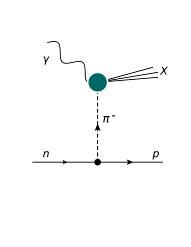
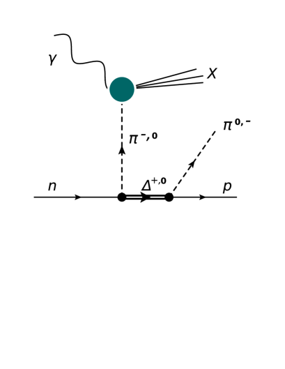
Figure 2: Representative processes contributing to single-inclusive production of forward protons off the neutron.

As it happens, for specific regions of kinematics, the observation of low-momentum recoil protons in the semi-inclusive reaction $eN\to eNX$ depicted (for select possibilities) in Fig. 2 can reveal features associated with correlated $q\bar{q}$ pairs in the nucleon, i.e., the nucleon’s pion cloud as just described. In particular, at low values of the $4$-momentum transfer squared $t\equiv k^{2}=(p-p^{\prime})^{2}\sim m^{2}_{\pi}$, where $p$ and $p^{\prime}$ are the initial and final nucleon $4$-momenta, the cross section displays behavior characteristic of pion pole dominance — akin to the behavior implied by the relation in Eq. (3) for exclusive electroproduction. In the DIS process at low $t$, contributions from exchanges of non-pseudoscalar quantum numbers ($J^{P}=0^{-}$), such as those of the $\rho$ meson and its isosinglet counterpart the $\omega$, are suppressed. That this must be the case is made plain in the analysis surrounding the right panel of Fig. 11, whereby we argued that the prodigious energy gap between the $\pi$ and $\rho$ masses suppresses the contribution of the latter to the $SU(2)$ Fock space expansion. Furthermore, the direct fragmentation of the scattered quark, or spectator “diquark” system that remains after a quark is pulled out of the nucleon, generally produces a considerably flatter $t$ dependence, which is qualitatively different from behavior near the pion pole.

This general behavior should permit a precise extraction of the pion cloud’s role in DIS from the nucleon, and we perform here some illustrative phenomenological computations that make this case; we do so by first exploring for context inclusive DIS in Sec. 1, before performing in Sec. 2 analogous calculations of semi-inclusive cross sections, where hadronic tagging of the final state may yield the desired information.

1 Pion cloud for inclusive DIS

Separate from its identity as a hadronic bound state, the pion may also be understood according to its status as the pseudo-Goldstone boson [228] associated with spontaneous breaking of QCD’s chiral symmetry. That nature confers upon chiral perturbation theory ($\chi$PT) as formulated in terms of pionic degrees of freedom considerable power in elucidating the dynamics of pion-nucleon interactions.

$\chi$PT specifies the appropriate pseudovector lagrangian for the pion-nucleon interactions [229] as

$${\cal L}_{\pi N} = {g_{A}\over 2f_{\pi}}\,\bar{\psi}_{N}\gamma^{\mu}\gamma_{5}\,\bm{\tau}\cdot\partial_{\mu}\bm{\pi}\,\psi_{N}\ -\ {1\over(2f_{\pi})^{2}}\,\bar{\psi}_{N}\gamma^{\mu}\,\bm{\tau}\cdot(\bm{\pi}\times\partial_{\mu}\bm{\pi})\,\psi_{N}\ ,$$ (6)

where the first term generates characteristic “rainbow” diagrams representing the dominant piece of the one-loop contribution to the nucleon wavefunction due to its ($N\rightarrow\pi N$) dissociations in the Sullivan process [226]. This contribution allows us to write the $SU(2)$ counterpart to Eq. (7) that we encountered in the $SU(4)$ flavor sector:

$$|N\rangle\ =\ \sqrt{Z_{2}}\,\left|N\right.\rangle_{0}\ +\ \sum_{M,B}\int\!dz\,f_{MB}(z)\,|M(z);B(1-z)\rangle\ ,$$ (7)

where the sum over states $(M,B)$ now runs over light hadrons represented by multiplets like the $s=0$ entries of Fig. 1; the resulting contribution to the inclusive $F_{2}$ structure function of the nucleon from scattering off a virtual pion emitted from the nucleon is therefore

$$F_{2}^{(\pi N)}(x)=\int_{x}^{1}dz\,f_{\pi N}(z)\ \cdot\ F_{2\pi}\Big{(}\frac{x}{z}\Big{)},$$ (8)

where $z=k^{+}/p^{+}$ is the light-cone momentum fraction of the initial nucleon carried by the interacting pion. For reasons of more general compatibility with the standing literature related to semi-inclusive production of final state protons, we resort to $z$, rather than $y$ for the light front momentum fraction $k^{+}/p^{+}$ as we had in Chap. 4. We point out that the second term of Eq. (6) produces four-point pion-nucleon vertices responsible for “bubble” diagrams that do not participate at $z\neq 0$; since the present study is mainly concerned with observable effects at finite $z$, we dispense with these contributions altogether. While this may be the case, the bubble diagrams generated by the second term of Eq. (6) do in fact contribute for $z\equiv 0$ — an important and largely uninvestigated consideration of consequence to sum rules like Eq. (5).

In the infinite momentum frame, the light-front definition $z=k^{+}/p^{+}$ coincides with the longitudinal momentum fraction, whereas in the rest frame of the target nucleon used in the subsequent treatment, $z$ is expressed as

$$z=\Big{(} k_{0}+|{\bm{k}}|\cos\theta\Big{)}\Big{/}M\ ,$$

$$k_{0}=M-\sqrt{M^{2}+{\bm{k}}^{2}}\ ,$$ (9)

where yet again $M$ is the mass of the nucleon, $k_{0}$ the pion energy, and $\theta$ is the angle between the vector $\bm{k}$ and the $z$-axis (which is equal to the angle between the recoil proton momentum ${\bm{p}}^{\prime}$ and the photon direction). For ease of notation, we also suppress the explicit dependence of the structure functions on the scale $Q^{2}$.

In this setting, the function $f_{\pi N}(z)$ gives the light-cone momentum distribution of pions in the nucleon [similar to Eq.(26)],

$$f_{\pi N}(z)=c_{I}\frac{g_{\pi NN}^{2}}{16\pi^{2}}\int_{0}^{\infty}\frac{dk^{2}_{\perp}}{(1-z)}\frac{G_{\pi N}^{2}}{z\ (M^{2}-s_{\pi N})^{2}}\left(\frac{k^{2}_{\perp}+z^{2}M^{2}}{1-z}\right),$$ (10)

where $k_{\perp}$ is the transverse momentum of the pion, $g_{\pi NN}$ is the $\pi NN$ coupling constant, and the isospin factor $c_{I}=1$ for $\pi^{0}$ ($p\to p\pi^{0}$ or $n\to n\pi^{0}$) and $c_{I}=2$ for $\pi^{\pm}$ ($p\to n\pi^{+}$ or $n\to p\pi^{-}$). The function $G_{\pi N}$ parametrizes the momentum dependence of the $\pi NN$ vertex function, which, due to the finite size of the nucleon, suppresses contributions from large-$|\bm{k}|$ configurations. Similar expressions may of course be written for various other contributions, such as those of $\rho$ mesons or involving $\Delta$ baryons in an intermediate state (e.g., the right panel of Fig. 2): we have already developed the required technology in Chap. 4 with Eqs. (35 & 40). However, because of the small mass of the pion, the $\pi N$ configuration is expected to be the dominant one as we demonstrate below through explicit calculation. Also, as in Chap. 4 the variable $s_{\pi N}=(k_{\perp}^{2}+m_{\pi}^{2})/z+(k_{\perp}^{2}+M^{2})/(1-z)$ of Eq. (10) represents the total squared center of mass energy of the intermediate $\pi N$ system, and is related to the pion virtuality $t$ by $t-m_{\pi}^{2}=z\cdot(M^{2}-s_{\pi N})$.

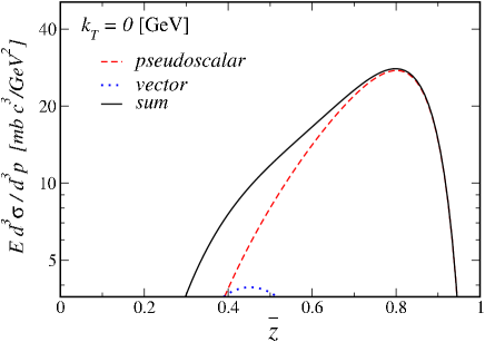
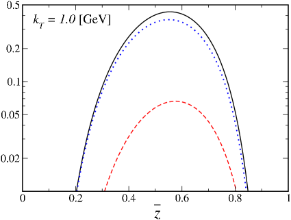
Figure 3: Typical spectra for the differential cross section $Ed^{3}\sigma/d^{3}p^{\prime}$ in the $pp\to nX$ reaction for transverse momentum $k_{\perp}=0$ (left) and $k_{\perp}=1$ GeV (right), as a function of the light-cone momentum fraction $\bar{z}\equiv 1-z$. The pseudoscalar $\pi$ (red dashed lines) and vector $\rho$ (blue dotted lines) contributions, and their sum (black solid lines), are indicated explicitly.

The form factor $G_{\pi N}$ (or more generally $G_{MN}$ for a meson $M$) can be constrained by comparing the pion cloud contributions with data on inclusive $pp\to nX$ scattering (akin to the ISR $\Lambda_{c}$ production data used to fit the analogous model parameters of Chap. 4.1), as performed by Holtmann et al. [195]. For the purpose of this penultimate chapter, we use the parametric form

$$G_{\pi N}=\exp\left[(M^{2}-s_{\pi N})/\Lambda^{2}\right],$$ (11)

where $\Lambda$ is the form factor cutoff parameter. (Note that in Ref. [195] a parametrization of the form $\exp[(M^{2}-s_{\pi N})/2\Lambda^{2}]$ is used, so that the corresponding cutoffs there are smaller by a factor of $\sqrt{2}$.) An illustration of the typical spectra for the differential cross section $Ed^{3}\sigma/d^{3}p^{\prime}$ in the $pp\to nX$ reaction arising from $\pi$ and $\rho$ exchange is shown in Fig. 3 as a function of the light-cone momentum fraction $\bar{z}\equiv 1-z$ carried by the final nucleon, for two values of the transverse momentum $k_{\perp}$. For small $k_{\perp}$ the $\pi$ exchange contribution clearly dominates at all $\bar{z}$, while at larger momenta the contributions from heavier mesons such as the $\rho$ become more important. Again, the specifics of this momentum dependent balance between pseudoscalar and vector exchange mechanisms is largely accounted for by the profile shown in the right panel of Fig. 11.

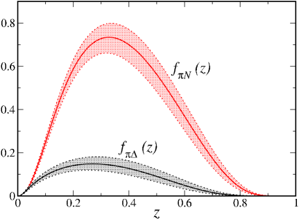
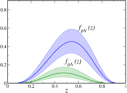
Figure 4: Light-cone momentum distributions of the pion, $f_{\pi N}$ and $f_{\pi\Delta}$ (left) and the $\rho$ meson, $f_{\rho N}$ and $f_{\rho\Delta}$ (right), as a function of the meson light-cone momentum fraction $z$. The error bands correspond to the cutoff parameter ranges as given in the text.

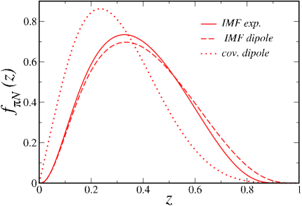
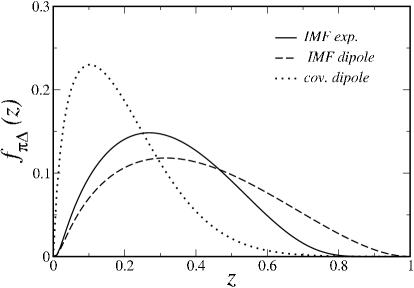
Figure 5: Light-cone momentum distributions for the $\pi N$ (left) and $\pi\Delta$ (right) intermediate states, for several different functional forms of the form factor $G$ in Eq. (10): “IMF” refers to $s$-dependent forms such as in Eq. (11), while “cov” denotes a form factor that depends only on the variable $t$.

Using cutoff parameters constrained by the inclusive hadronic $pp\to nX$ data, which were found in Ref. [195] and reproduced here as $\Lambda_{\pi N}=\Lambda_{\rho N}=1.56\pm 0.07$ GeV and $\Lambda_{\pi\Delta}=\Lambda_{\rho\Delta}=1.39\pm 0.07$ GeV, the light-cone momentum distributions $f(z)$ are shown in Fig. 4. The principal model uncertainty in these results comes from the ultraviolet regulator $G_{MN}(s)$ used to truncate the $k_{\perp}$ integrations in the distribution functions. Various functional forms have been advocated in the literature aside from the $s$-dependent exponential form factor in Eq. (11), and we compare several of these, including $s$- and $t$-dependent dipole forms) in Fig. 5. For the $s$- and $t$-dependent forms in particular, the differences are noticeable mostly at small values of $z$, where the $t$-dependent parametrization (of the form $G\sim 1/(t-\Lambda^{2})^{2}$) gives somewhat larger distributions that are peaked at smaller $z$ compared to the $s$-dependent form, which tend to be broader.

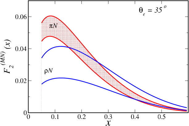
Figure 6: Contributions from $\pi N$ and $\rho N$ intermediate states to the inclusive $F_{2}$ structure function of the proton for a typical fixed electron scattering angle.

Convoluting the light-cone distributions with the structure function of the meson as in Eq. (8), the resulting contributions from the $\pi N$ and $\rho N$ intermediate states to the inclusive $F_{2}$ structure function of the proton are illustrated in Fig. 6. For the meson structure function we use a parametrization from GRV [230], and assume $F_{2\pi}(x)\approx F_{2\rho}(x)$. The results are plotted for a plausible value of the scattering angle of the final state electron $\theta_{e}\sim 35^{\circ}$, which determines the $Q^{2}$ dependence of the contribution at a given $x$ via a few simple manipulations of the DIS definitions given in Chap. 1.1:

$$Q^{2}\ =\ 2xME\ \left\{1\ -\ \left({2E\over xM}\sin^{2}{{\theta_{e}\over 2}}\ +\ 1\right)^{-1}\right\}\ .$$ (12)

We thus find that for typical lepton scattering angles at, e.g., JLab with $E=11$ GeV, the sensitivity to $Q^{2}$ is rather small at shallow $x\lesssim 0.2$ due to the mild scale dependence of the meson structure functions used. For the fully integrated results of Fig. 6, the model uncertainties are greatest for the lowest accessible values of $x\sim 0.05$; depending upon choice of the phenomenological cutoff parameter $\Lambda$, the $\pi$ contribution to $F_{2}$ can either be comparable to that of the $\rho$, or even larger at high values of $x$ (where the calculation is also less reliable).

2 Tagged structure functions

While the inclusive reactions require integration of the pion momentum over all possible values, detecting — “tagging” — the recoil proton in the final state allows one to dissect the internal structure with significantly more detail and increase the sensitivity to the dynamics of the meson exchange reaction; this is attributable to the fact that final state tagging effectively isolates contributions of the type shown in Fig. 2 in specific kinematical bins of produced hadron momenta, angle, etc. Our interests lie foremost in the relative contributions of the semi-inclusive reaction with respect to the inclusive process. In practice, the semi-inclusive structure function will be given by the unintegrated product

$$F_{2}^{(\pi N)}(x,z,k_{\perp})=f_{\pi N}(z,k_{\perp})\ \cdot\ F_{2\pi}\Big{(}\frac{x}{z}\Big{)}\ ,$$ (13)

where the unintegrated distribution function $f_{\pi N}(z,k_{\perp})$ is defined by

$$f_{\pi N}(z)={1\over M^{2}}\int_{0}^{\infty}dk^{2}_{\perp}\ f_{\pi N}(z,k^{2}_{\perp})\ .$$ (14)

The dependence of the tagged structure functions on the kinematical variables that are measured experimentally can be studied by relating the magnitude of the 3-momentum ${\bm{k}}$ of the exchanged pion in the target rest frame to the pion’s transverse momentum $k_{\perp}$ and light-cone fraction $z$,

$$\bm{k}^{2} =k^{2}_{\perp}+k^{2}_{\parallel}$$

$$=k^{2}_{\perp}+\frac{\left[k^{2}_{\perp}+(1-[1-z]^{2})M^{2}\right]^{2}}{4M^{2}(1-z)^{2}}\ .$$ (15)

Experimentally, the quantities most readily measured are the momentum of the produced proton, ${\bm{p}^{\prime}}$, which in the rest frame is ${\bm{p}^{\prime}}=-\bm{k}$, and the scattering angle $\theta_{p^{\prime}}$ of the final state proton with respect to the virtual photon direction. In the limit $k^{2}_{\perp}=0$, the magnitude of ${\bm{k}}$ becomes

$$|\bm{k}|_{k^{2}_{\perp}=0}=\frac{zM}{2}\left(\frac{2-z}{1-z}\right)\ ,$$ (16)

which imposes the restriction $z\lesssim|\bm{k}|/M$. This relation is illustrated in Fig. 7 for values of $z$ up to 0.2, and establishes the bound placed upon the momentum fraction $z$ imposed by the soft limit proximate to the $t=+m^{2}_{\pi}$ pole.

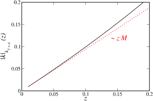
Figure 7: Pion momentum $|\bm{k}|$ as a function of the light-cone fraction $z$ for $k_{\perp}=0$ (black solid). The linear approximation $\sim zM$ (red dotted) is shown for comparison.

This kinematic restriction on $|\bm{k}|$ for a given $z$ can also be illustrated by considering the unintegrated light-cone distribution functions as a function of the variable $t$. This is relevant since one way of identifying the pion exchange mechanism is through its characteristic $t$ dependence, which is pronounced near the pion pole. The production of a physical proton (or $\Delta$ baryon) in the final state restricts the maximum value of $t$, however (corresponding to the minimum transverse momentum, $k_{\perp}=0$), to

$$t^{N}_{\rm max}=-{M^{2}z^{2}\over 1-z}\ ,\ \ \ \ t^{\Delta}_{\rm max}=-{\left(M_{\Delta}^{2}-(1-z)M^{2}\right)z\over 1-z}\ ,$$ (17)

for final state nucleons $N$ and intermediate $\Delta$ states, respectively. Implementing these limits, the $t$-dependence of the distributions for $\pi$ exchange with a nucleon or $\Delta$ recoil is illustrated in Fig. 8. Note that at the larger $z$ value there is a considerable gap between the values of $t$ at which $\Delta$ production is possible compared with $N$ production.

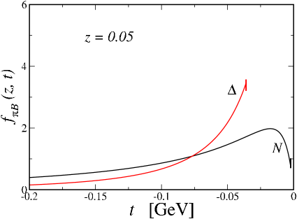
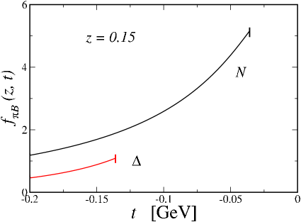
Figure 8: Unintegrated light-cone distribution functions for $\pi N$ (black solid) and $\pi\Delta$ (red solid) states as a function of $t$, for fixed values of $z=0.05$ (left) and $z=0.15$ (right).

The most judicious way of proceeding experimentally would then be to measure the semi-inclusive cross section in specific bins of recoil proton momentum $|\bm{p}^{\prime}|=|\bm{k}|$ and scattering angle $\theta_{p^{\prime}}$ (or equivalently $z$ and $k_{\perp}$). For this purpose, we hence define a partially integrated semi-inclusive structure function $F_{2}^{(\pi N)}(x,\Delta z,\Delta k_{\perp}^{2})$,

$$F_{2}^{(\pi N)}(x,\Delta z,\Delta k_{\perp}^{2})={1\over M^{2}}\int_{\Delta z}dz\int_{\Delta k_{\perp}^{2}}dk^{2}_{\perp}\ f_{\pi N}(z,k_{\perp})\ \cdot\ F_{2\pi}\Big{(}\frac{x}{z}\Big{)}\ ,$$ (18)

integrated over the range $\Delta z=[z_{\rm min},z_{\rm max}]$ and $\Delta k_{\perp}^{2}=[k_{\perp\rm min}^{2},k_{\perp\rm max}^{2}]$. Of course, this is composed in the “theory” space spanned by $(z,k^{2}_{\perp})$, and lab frame expressions would be preferred; one can therefore translate to an alternative expression for the semi-inclusive structure function integrated over the target-frame variables $|\bm{k}|$ and $\theta_{p^{\prime}}$. With this, we shall evaluate, e.g.,

$$F_{2}^{(\pi N)}(x,\Delta|{\bm{k}}|,\Delta\theta_{p^{\prime}})={1\over M^{2}}\int_{\Delta|{\bm{k}}|}d|{\bm{k}}|\int_{\Delta\theta_{p^{\prime}}}d\theta_{p^{\prime}}\ J(x,|{\bm{k}}|,\theta_{p^{\prime}})\ \cdot\ f_{\pi N}(\tilde{z},\tilde{k}_{\perp})\,F_{2\pi}\Big{(}\frac{x}{\tilde{z}}\Big{)}\ ,$$ (19)

where now $\Delta|{\bm{k}}|=[|{\bm{k}}|_{\rm min},|{\bm{k}}|_{\rm max}]$, $\Delta\theta_{p^{\prime}}=[\theta_{p^{\prime}}^{\rm min},\theta_{p^{\prime}}^{\rm max}]$, and the Jacobian appropriate to the lab-frame transformations

$$\tilde{z}(|{\bm{k}}|,\theta_{p^{\prime}})\ =\ {1\over M}|{\bm{k}}|\cos{\theta_{p^{\prime}}}\ +\ {1\over M}\left(M-\sqrt{M^{2}+|{\bm{k}}|^{2}}\right)$$ (20a)

$$\tilde{k}_{\perp}(|{\bm{k}}|,\theta_{p^{\prime}})\ =\ |{\bm{k}}|\sin{\theta_{p^{\prime}}}$$ (20b)

can be put down as

$$J(x,|{\bm{k}}|,\theta_{p^{\prime}})\ \mathrel{\vbox{\hbox{\scriptsize.}\hbox{\scriptsize.}}}=\ {\partial(x,\tilde{z},\tilde{k}^{2}_{\perp})\over\partial(x,|{\bm{k}}|,\theta_{p^{\prime}})}$$

$$=\ {2\over M}|{\bm{k}}|^{2}\sin{\theta_{p^{\prime}}}\left(1-\sin{\phi_{k}}\cdot\cos{\theta_{p^{\prime}}}\right)\ ,$$ (21)

and we have defined the parameter $\phi_{k}\mathrel{\vbox{\hbox{\scriptsize.}\hbox{\scriptsize.}}}=\tan^{-1}(|{\bm{k}}|/M)$. JLab experiments such as that proposed in [225] promise to probe the kinematical ranges $0.05\lesssim z\lesssim 0.2$ and $60\lesssim|\bm{k}|\lesssim 400$ MeV, and angles $30^{\circ}\lesssim\theta_{p^{\prime}}\lesssim 160^{\circ}$, with $x$ in the vicinity of $x\sim 0.05-0.2$, wherein we trace some of the more salient signals for DIS from the nucleon’s pion cloud using tagged structure functions such as Eq. (19).

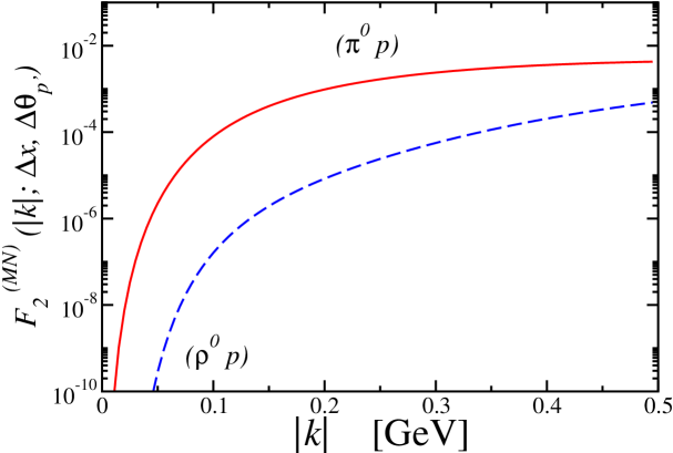
Figure 9: Semi-inclusive structure functions $F_{2}^{(MN)}(|{\bm{k}}|;\Delta x,\Delta\theta_{p^{\prime}})$ over an illustrative range for $|{\bm{k}}|$ up to 0.5 GeV for the $p\to M\,p$ process, with $M=\pi^{0}$ (red solid) and $M=\rho^{0}$ (blue dashed), as a function of the recoil proton momentum $|{\bm{k}}|$, integrated over $\Delta x=[0,0.6]$ and all angles $\theta_{p^{\prime}}$.

To that end, Fig. 9 shows the semi-inclusive structure functions$F_{2}^{(MN)}(|{\bm{k}}|;\Delta x,\Delta\theta_{p^{\prime}})$ for the neutral-exchanges $p\to\pi^{0}\,p$ and $p\to\rho^{0}\,p$, as a function of the momentum $|{\bm{k}}|$, integrated over $x$ between 0 and 0.6, and over all angles $\theta_{p^{\prime}}$ from 0 to $\pi$. The $\rho$ contribution is clearly suppressed relative to the pion contribution, with the structure functions rising steadily at increasing $|{\bm{k}}|$ in the sampled region $|{\bm{k}}|\lesssim 0.5$ GeV. At larger momenta, beyond the kinematic region plotted in Fig. 9, the effects of the meson–nucleon form factors become more important, eventually suppressing the contributions from high-$|{\bm{k}}|$ tails of the distributions. The peak in the $\pi$ distribution occurs at $|{\bm{k}}|\approx 0.6$ GeV, while the $\rho$ distribution peaks at higher momenta, $|{\bm{k}}|\approx 1.2$ GeV, and has a slower fall-off with $|{\bm{k}}|$.

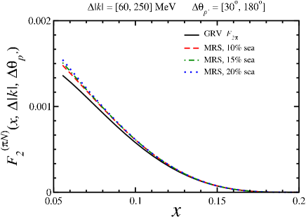
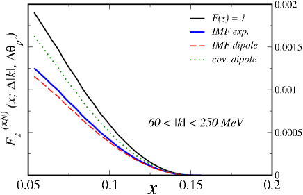
Figure 10: (Left) Semi-inclusive structure function $F_{2}^{(\pi N)}(x,\Delta|{\bm{k}}|,\Delta\theta_{p^{\prime}})$ for the $p\to\pi^{0}\,p$ process, integrated over the momentum range $\Delta|{\bm{k}}|=[60,250]$ MeV and angular range $\Delta\theta_{p^{\prime}}=[30^{\circ},180^{\circ}]$. The results with the GRV [230] (black solid) parametrization of the pion structure function are compared with those using the MRS [231] fit with different amounts of sea, 10% (red dashed), 15% (green dot-dashed) and 20% (blue dotted). (Right) The same quantity, but now examining the variations due to different choices for the vertex form factor $G_{\pi N}$, as explicitly indicated above.

The dependence of the semi-inclusive structure function $F_{2}^{(\pi N)}(x,\Delta|{\bm{k}}|,\Delta\theta_{p^{\prime}})$ on the pion structure function parametrization is shown in the left of Fig. 10 as a function of $x$, integrated over the proposed momentum range $\Delta|{\bm{k}}|=[60,250]$ MeV and angular range $\Delta\theta_{p^{\prime}}=[30^{\circ},180^{\circ}]$. The results with the GRV parametrization [230] of the pion parton distribution functions are compared with those using the MRS parametrization [231] with different amounts of sea, ranging from 10% to 20%. The pion structure function is relatively well constrained from pion–nucleon Drell-Yan data at Fermilab at intermediate and large values of $x$, but is not as well determined at small $x$ values.

Nevertheless, the variation in the computed semi-inclusive proton structure function from uncertainties in the pion distribution functions is quite small, and considerably smaller than the uncertainties from the pion–nucleon vertex form factor dependence, which is illustrated in the right panel of Fig. 10. Specifically, we exhibit the semi-inclusive structure functions as a function of $x$ and integrated over the momentum range $\Delta|\bm{k}|=[60,250]$ MeV; we compare the $s$-dependent (IMF) exponential and dipole form factors with the $t$-dependent dipole form factor, as well as with a calculation without any form factor suppression. In this case, the comparatively wide spread in predictions for the $x$ dependence corresponding to different scenarios for the $G_{\pi N}$ vertex suggests that this element of the calculation is indeed the least under control, and would benefit most from experimental guidance from direct measurement as might come from [225]. For instance, while the computation of $F^{(\pi N)}_{2}$ is apparently fairly insensitive to the specific functional form employed for the vertex form factor in the IMF, the more general choice of $s$ vs. $t$-dependent parametrizations is quite significant, being responsible for a $\sim$30% systematic effect at lower $x$.

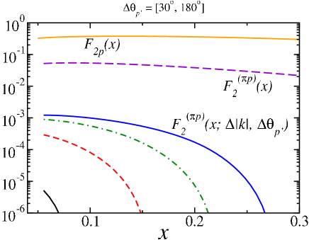
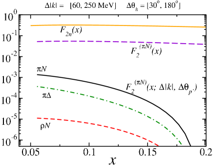
Figure 11: (Left) $x$ dependence of the semi-inclusive structure function $F_{2}^{(\pi p)}(x,\Delta|{\bm{k}}|,\Delta\theta_{p^{\prime}})$. For comparison, the total integrated $\pi p$ contribution $F_{2}^{(\pi p)}$ to the inclusive proton structure function is shown (violet dashed), as is the total inclusive $F_{2p}$ structure function (orange solid).The lower bands follow from varying the integration range $\Delta|{\bm{k}}|$ as described in the text. (Right) The corresponding quantity for charge-exchange in the $n\to\pi^{-}\,p$ process. The tagged semi-inclusive structure function for $(\pi^{-}p)$ (black, solid), $(\rho^{-}p)$ (red, dashed), and $(\pi^{0}\Delta^{0}+\pi^{-}\Delta^{+})$ (green, dot-dashed) are compared with the inclusive structure function of the neutron $F_{2n}(x)$ (orange), and the fully-integrated $(\pi^{-}p)$ contribution $F_{2}^{\pi N}(x)$ (violet, dashed).

Lastly, in Fig. 11 we predict the $x$ dependence for $F_{2}^{(\pi p)}(x,\Delta|{\bm{k}}|,\Delta\theta_{p^{\prime}})$ in several of the kinematical ranges we have proposed involving the charge-neutral process. First, in the LHS of Fig. 11 the colorful bands at bottom follow from varying the integration range $\Delta|{\bm{k}}|$; namely, they correspond to $\Delta|{\bm{k}}|=[60,100]$ MeV (black, solid), $\Delta|{\bm{k}}|=[100,200]$ MeV (red, dashed), $\Delta|{\bm{k}}|=[200,300]$ MeV (green, dot-dashed), and $\Delta|{\bm{k}}|=[300,400]$ MeV (blue, solid). While these steps in the integration range for $|{\bm{k}}|$ are fairly modest, the momentum dependence characterized in the preceding discussion induces large, order-of-magnitude separations among the results for various $|{\bm{k}}|$ intervals. At the same time, these observables are admittedly overshadowed by the much larger inclusive structure functions, which are given for comparison, but current and future facilities promise a high level of sensitivity. For instance, with a relatively standard initial run, the JLab measurement proposed in [225] should be sensitive to tagged structure functions down to $F_{2}^{(\pi p)}\sim 10^{-5}$.

That these measurements have the capacity to cleanly disentangle the role of scattering from the pion cloud is made evident by the complementary information shown in the right panel of Fig. 11, which is plotted for the charge exchange process $(n\rightarrow\pi^{-}p)$. As had already been hinted in Fig. 9, $\pi$-exchange is the dominant meson cloud process, eclipsing the corresponding mechanism involving the $\rho$ by $\sim 2$ orders of magnitude, even at the modest integration ranges shown, namely, $\Delta|{\bm{k}}|=[60,250]$ MeV and $\Delta\theta_{p^{\prime}}=[30^{\circ},180^{\circ}]$. Contributions from scattering via channels that consist of intermediate $\Delta$ baryons are midway between these two scenarios, being suppressed by an approximate order of magnitude relative to the simpler reaction shown in the left diagram of Fig. 2. Of course, in the absence of direct coincidence measurements of final state pions produced by the decay of the $\Delta$ (RHS of Fig. 3), these processes interfere, though the doubly-inclusive detection of a final state proton and pion may allow the structure of the $\Delta$ to be better isolated.

These demonstrations emphasize the accessibility of the nucleon’s pion cloud at a level which heretofore had been unprecedented. Computing within the ambitious but achievable kinematics outlined in this chapter, measurements have the novel ability to separate the contributions shown in Fig. 2 from various background processes, and better control their momentum dependence with sufficient resolution in $|{\bm{k}}|$ (as established by the LHS of Fig. 11). Moreover, with these resolution enhancements, measurements of cloud contributions can in principle be made very near the coveted $t=m^{2}_{\pi}$ pion pole as shown in Fig. 8; much same, this would also constrain the model dependence associated with the detailed behavior of the pion-nucleon vertex shown in Fig. 10 — information that would significantly clarify the pion cloud’s role in the structure of the interacting nucleon.

Chapter 6 Conclusion

“Reasoning draws a conclusion, but does not make the conclusion certain, unless the mind discovers it by the path of experience.”
      — Roger Bacon

This thesis has chiefly been concerned with hadronic structure as a nonperturbative problem — one that defies ready explanation in terms of the standard QCD interactions introduced in Chap. The nonperturbative structure of hadrons that have so successfully guided work at higher energies. In the course of investigation, we have in fact seen these nonperturbative properties to encompass an enormous range of phenomenology, and require dedicated theoretical effort on many fronts to make even halting progress. In spite of sustained attention, much remains fundamentally mysterious, and, true to form, improved understanding if anything only leads to more and deeper questions.

With the formal description in Chap. 1 of the DIS process and operator structure of inclusive scattering, we were launched upon this study by the dual recognition of the Compton amplitude’s ability to provide new information regarding the quark substructure of the nucleon (Chap. 1.2), and the problematic aspects of performing DIS measurements at intermediate $Q^{2}$ (Chap. 2). In the latter case, we noticed that parity-violating DIS is uniquely adapted as a tool to study novel aspects of the partonic structure of the nucleon, including the flavor dependence of PDFs in the region $x\sim 1$ or quark-level charge-symmetry violation, to say nothing of more exotic physics beyond the Standard Model.

While the numerical suppression of the leptonic vector couplings $C_{2q}$ relative to the axial-vector couplings $C_{1q}$ is the main culprit in the dominance of the hadronic-vector term $a_{1}$ inside the parity-violating asymmetry $A^{\rm PV}$, we observed that the axial-vector $a_{3}$ contribution can amount to as much as 20% of the total; the fact that this occurs for both proton and deuteron targets, and in particular, introduces dependence on the still somewhat uncontrolled electromagnetic ratio $R^{\gamma}$, implies that work remains in quantitatively understanding the vector/axial-vector separation of $A^{\rm PV}$.

A perhaps greater concern unique to the nonperturbative, low-$Q^{2}$ regime of DIS comes from the interference ratio $R^{\gamma Z}$, which enters through the larger $C_{1q}$-weighted vector term. Given its entirely unexplored phenomenology, $R^{\gamma Z}$ may well contribute to $A^{\rm PV}_{p}$ if it differs significantly from $R^{\gamma}$. We found that even modest deviations away from $R^{\gamma Z}\approx R^{\gamma}$ could potentially obscure the main physics objectives of DIS on the proton and deuteron — namely, enhanced access to flavor information (e.g., the $d/u$ PDF ratio) and quark-level CSV, respectively; this fact makes a more thorough understanding of $R^{\gamma Z}$ and related finite-$Q^{2}$ effects a matter of some urgency. Regarding the direct measurement of partonic CSV, we postulated an alternative mechanism in Chap. 2.3 involving $ed$ scattering mediated by $W$-exchange; using a framework partly based on electromagnetically induced CSV, we concluded a multi-percent signal could be observable at a TeV-scale electron-ion collider — yet another elusive physics objective such a machine might advance.

Work on the possible extension of these considerations to the domain of spin-polarized physics [148, 149, 150, 151] remains in its early stages, though we highlighted in Chap. 2.2 some suggestive ideas. The true push would be to reduce the uncertainties on the spin-dependent quark distributions, which remain quite egregious; for this purpose, new inputs from high precision PVDIS spin asymmetry measurements would obviously be invaluable.

Prodded forward by the potential importance of the largely uncontrolled ratio $R^{\gamma Z}$, we found a better understanding of the nonperturbative contributions to that quantity necessary in order to be more disposed in making definitive conclusions about its role in PVDIS. Among the more accessible effects in this wise are the target mass corrections, which we considered in both fully- and semi-inclusive reactions. While the nature of the deuteron as an isoscalar target insulates it from significant corrections from mass effects, this is much less the case for the proton, which experiences a multi-percent correction in both the asymmetry $A^{\rm PV}$ and the phenomenological ratio $R^{\gamma Z}$. For the latter, model dependence remains a serious issue, and a motivation for additional calculation and measurement.

In the future, additional effects may need to be considered at large $x$, not least of which are dynamical higher twist corrections associated with nonperturbative multi-parton correlations. These are of course very difficult to compute from first principles, and until the present time, only rudimentary model estimates have been available. Despite this limitation, our results on the phenomenology of the target mass corrections should provide a benchmark for future theoretical and experimental investigations of these additional corrections.

As for the hadron mass corrections to semi-inclusive processes we studied in Chap. 3.4, their most immediate use would be in leading twist analyses of SIDIS cross sections, for which such corrections are an unavoidable consideration before reliable extractions of parton distribution and fragmentation functions can be made at large $x$ and $z_{h}$. Clear applications of this work are also to be found in analyses of semi-inclusive data in the nucleon resonance region, which has been the recent focus of attention for the sake of understanding quark-hadron duality [169, 170, 171].

While the analysis of Chap. 3 was kept strictly to leading order in $\alpha_{s}$, an extended formalism at NLO is becoming more of a crying necessity; such a treatment is all the more imperative due to the current lack of a more quantitative description of transverse mass dependence of the produced hadrons, $p_{h\perp}\neq 0$. Such an improvement would indubitably be a great service to on-going studies of the Sivers, Boer-Mulders, and other effects related to transverse momentum dependent parton distributions (TMDs), in which nonzero parton transverse momentum, $k_{\perp}\neq 0$, is a defining feature.

At the same time, unresolved challenges in the formalism itself remain. This is clear given that the corrected SIDIS cross section still exhibits the threshold problem which renders it nonzero as $x\to x^{\rm max}$, much as we saw for inclusive DIS. Solutions of this problem proposed in the literature for inclusive structure functions [154, 155, 159] must be extended to SIDIS in future work.

Throughout the analysis of Chaps. 2–3 we assumed (as is in fact the case) that the electroweak structure functions are dominated in the QPM by their light $(u,d,s)$ degrees of freedom. In this thesis’ spirit of accounting for potential signals of nonperturbative dynamics at large $x$ and moderate $Q^{2}$, Chap. 4 presented a comprehensive analysis of intrinsic charm in the nucleon using a phenomenological model formulated in terms of effective meson–baryon degrees of freedom; in doing so, we derived couplings from $DN$ and $\bar{D}N$ Lippmann-Schwinger analyses [187, 188, 189], which permitted us to constrain model parameters in the form of ultraviolet regulators using hadroproduction data [191] and consistency checks [192].

In stark contrast to previous studies that neglected the spin structure [180] and assumed dominance by the lowest mass state [178, 179], we included all low-lying hadrons of the $SU(4)$ spectrum in an ansätz that directly connects the properties of the bound state spectrum to the multiplicity and momentum dependence of the underlying charm quarks. Additionally, it was necessary to model internal distributions for $c$ and $\bar{c}$ quarks within the charmed baryons and mesons, and this was accomplished by means of a relativistic quark–spectator model, in which the momentum distributions of the quarks are parametrized through phenomenological quark–spectator–nucleon vertex functions. This procedure involved a number of assumptions, and we therefore compared several numerical approaches to understand the systematic sources of model dependence. While this permitted a range of final shapes for charm and anticharm momentum distributions, we turned to the technology of QCD global analysis to further constrain the overall normalization of the intrinsic charm multiplicity. Keeping a special eye to SLAC $ep$ and $ed$ data at $Q^{2}\gtrsim 1$ GeV² and $W^{2}\gtrsim 3.5$ GeV² [213], the fits presented in Chap. 4.4 strongly constrained the momentum carried by intrinsic charm; in the absence of high-$x$ $F^{c}_{2}$ measurements from EMC, we found a quite restrictive upper bound, $\langle x\rangle_{\rm IC}\leq 0.1$% at the $5\sigma$ level, though fits that do include EMC data favor a rather small intrinsic charm component, $\langle x\rangle_{\rm IC}=0.13\pm 0.04$%.

In the end, however, direct charm production data at high $x$ and moderate $Q^{2}$ would have the most immediate bearing on the intrinsic charm question, and such measurements would advance this topic markedly. One might proceed experimentally by searching for the characteristic asymmetries in the $x$ dependence of the $c$ and $\bar{c}$ distributions (or analogously, charge asymmetries in the hadroproduction of, e.g., $D^{+}/D^{-}$ or $\Lambda_{c}/\bar{\Lambda}_{c}$), that are an inevitable consequence of MBMs such as the one presented in Chap. 4. Slightly more indirect channels might also be of use: for instance, the measurement of $W$ and $Z$ cross sections at the LHC [207], which receive significant contributions from charm production, or photon plus charm jet production, also at LHC kinematics [208].

Extension in a more detailed fashion to the strange $SU(3)$ sector (which possesses more plentiful data in specific meson and baryon production channels), as well as confrontation with new charm production data that might emerge from an eventual electron-ion collider would aid in gauging the reliability of some of the model assumptions made in Chap. 4 — particularly regarding the truncation of the Fock state expansion of Eq. (7).

Finally, in Chap. 5 we provided further phenomenological justification for the Fock state expansion of the nucleon used in Chap. 4, exploiting the spontaneously broken chiral symmetry of QCD as motivation for modeling the nucleon’s “pion cloud.” This effect provides an avenue to precise intermediate $Q^{2}$ determinations of both the much-sought pion form factor $F_{\pi}$, and, as we demonstrated for a proposed JLab experiment [225], the DIS structure function $F^{\pi}_{2}$. These measurements stand to improve the connection between the pion as a pseudo-Goldstone boson and its light quark substructure — a relationship that has been the subject of numerous modeling efforts, but as always, requires experimental input to constrain the diverse range of predictions.

Several of the author’s scientific publications have contributed to this thesis with permission.

• T. Hobbs and W. Melnitchouk,
        Phys. Rev. D 77, 114023 (2008) [arXiv:0801.4791 [hep-ph]].
        Finite-$Q^{2}$ corrections to parity-violating DIS.
        Copyright 2008 by the American Physical Society.

• A. Accardi, T. Hobbs and W. Melnitchouk,
        JHEP 0911, 084 (2009) [arXiv:0907.2395 [hep-ph]].
        Hadron mass corrections in semi-inclusive deep inelastic scattering.

• T. J. Hobbs, J. T. Londergan, D. P. Murdock and A. W. Thomas,
        Phys. Lett. B 698, 123 (2011) [arXiv:1101.3923 [hep-ph]].
        Testing Partonic Charge Symmetry at a High-Energy Electron Collider.
        Copyright 2011 by Elsevier.

• L. T. Brady, A. Accardi, T. J. Hobbs and W. Melnitchouk,
        Phys. Rev. D 84, 074008 (2011) [arXiv:1108.4734 [hep-ph]].
        NLO analysis of target mass corrections to structure functions and asymmetries.
        Copyright 2011 by the American Physical Society.

• M. Gorchtein, T. Hobbs, J. T. Londergan and A. P. Szczepaniak,
        Phys. Rev. C 84, 065202 (2011) [arXiv:1110.5982 [nucl-th]].
        Compton Scattering and Photo-absorption Sum Rules on Nuclei.
        Copyright 2011 by the American Physical Society.

• T. J. Hobbs, J. T. Londergan and W. Melnitchouk,
        Phys. Rev. D 89, 074008 (2014) [arXiv:1311.1578 [hep-ph]].
        Phenomenology of nonperturbative charm in the nucleon.
        Copyright 2014 by the American Physical Society.

• P. Jimenez-Delgado, T. J. Hobbs, J. T. Londergan and W. Melnitchouk,
        arXiv:1408.1708 [hep-ph].
        New limits on intrinsic charm in the nucleon from global analysis of parton distributions.

• A. Camsonne, et al.,
        Jefferson Lab Proposal PR12-14-010, (2014).
        Measurement of Tagged Deep Inelastic Scattering (TDIS).

CURRICULUM VITAE

Timothy John Hobbs          timjhobb@indiana.edu          Citizenship: USA

Education

• Ph.D. Physics (Nuclear/HEP theory), Indiana University, August 2014.
  Thesis: The Nonperturbative Structure of Hadrons;
  advisor(s): J. Timothy Londergan and Wally Melnitchouk.

• M.S. Physics, Indiana University, December 2010.

• B.A. Physics, The University of Chicago, June 2009.
  Thesis: Oblique Corrections in Electroweak Physics;
  advisor: Jon Rosner.

• B.A. Mathematics, The University of Chicago, June 2009.

Teaching Experience

Associate Instructor at Indiana University:

• (Grading), Physics 453 (Quantum Mechanics)
  Spring 2012

• (Laboratory), Physics 202 (Introductory Electricity & Magnetism)
  Fall/Spring 2011/12

• (Recitation), Physics 221/2 (Calculus-based Mechanics/Electricity-Magnetism)
  Fall/Spring 2010/11

• (Laboratory), Physics 201 (Introductory Mechanics)
  Fall/Spring 2009/10

Journal Articles

1. T. J. Hobbs, Chueng-Ryong Ji, J. T. Londergan and W. Melnitchouk
   in progress:
   The role of the Delta in relativistic pion loop corrections to photon-nucleon vertices

2. T. J. Hobbs, P. Jimenez-Delgado, J. T. Londergan and W. Melnitchouk
   Phys. Rev. Lett. (submitted), [arXiv:1408.1708 [hep-ph]]:
   New limits on intrinsic charm in the nucleon from global analysis of parton distributions

3. T. J. Hobbs, J. T. Londergan and W. Melnitchouk
   Phys. Rev. D 89, 074008 (2014), [arXiv:1311.1578 [hep-ph]]:
   Phenomenology of nonperturbative charm in the nucleon

4. M. Gorchtein, T. Hobbs, J. T. Londergan and A. P. Szczepaniak
   Phys. Rev. C 84, 065202 (2011), [arXiv:1110.5982 [nucl-th]]:
   Compton Scattering and Photo-absorption Sum Rules on Nuclei

5. L. T. Brady, A. Accardi, T. J. Hobbs and W. Melnitchouk
   Phys. Rev. D 84, 074008 (2011), [arXiv:1108.4734 [hep-ph]]:
   Next-to leading order analysis of target mass corrections to structure functions and asymmetries

6. T. J. Hobbs, J. T. Londergan, D. P. Murdock and A. W. Thomas
   Phys. Lett. B 698, 123 (2011), [arXiv:1101.3923 [hep-ph]]:
   Testing Partonic Charge Symmetry at a High-Energy Electron Collider

7. T. Hobbs and J. L. Rosner
   Phys. Rev. D 82, 013001 (2010), [arXiv:1005.0797 [hep-ph]]:
   Electroweak Constraints from Atomic Parity Violation and Neutrino Scattering

8. A. Accardi, T. Hobbs and W. Melnitchouk
   JHEP 0911, 084 (2009), [arXiv:0907.2395 [hep-ph]]:
   Hadron mass corrections in semi-inclusive deep inelastic scattering

9. T. Hobbs and W. Melnitchouk
   Phys. Rev.  D 77, 114023 (2008), [arXiv:0801.4791 [hep-ph]]:
   Finite-Q² corrections to parity-violating DIS

Talks and Conferences

• Invited talk: “Phenomenological implications of the nucleon’s meson cloud” at the Light Cone 2014 International Workshop, Raleigh, NC; May 27, 2014.

• Invited seminar(s): “Nonperturbative aspects of hadron structure phenomenology” at the University of Washington Nuclear Theory Group, Seattle, WA; January 30, 2014 AND the Argonne National Lab Physics Division Theory Group, Lemont, IL; February 11, 2014.

• Invited talk: “Numerical estimates of chiral cloud contributions to tagged proton electroproduction” at the JLab workshop “Exploring Hadron Structure with Tagged Structure Functions,” Newport News, VA; January 16-18, 2014.

• Contributed talk: “Phenomenology of nonperturbative heavy quarks in the nucleon” at the 2013 Fall Meeting of the APS Prairie Section, Columbia, MO; November 7-9, 2013.

• Contributed talk: “Comparative study of nonperturbative heavy quarks in the nucleon” at the 2013 DNP Meeting, Newport News, Virginia; October 23-26, 2013.

• Contributed talk: “Nonperturbative heavy quarks in the nucleon” at the 26^th Annual Midwest Theory Get-Together, Argonne National Lab; September 6 & 7, 2013.

• Contributed poster: “Nonperturbative charm content of the nucleon” EPJ Web of Conf. 66, 06007 (2014) [INPC 2013]; at the 2013 International Nuclear Physics Conference, Firenze, Italy; June 2-7, 2013.

• Invited talk: “Non-perturbative (and perturbative) charm contributions to various processes” at the 5th Workshop of the APS Topical Group on Hadronic Physics, Denver, Colorado; April 10-12, 2013.

• Contributed talk: “Intrinsic charm of the proton” at the 25^th Annual Midwest Theory Get-Together, Argonne National Lab; September 7 & 8, 2012.

• Invited talk: “Non-perturbative charm content of the nucleon” at the International Workshop on “Physics Opportunities at an Electron-Ion Collider,” held at Indiana University, Bloomington; August 20-22, 2012.

• Contributed talk: “Partonic charge symmetry violation at LHC kinematics” at the 24^th Annual Midwest Theory Get-Together, Argonne National Lab; September 23 & 24, 2011.

• Contributed talk/poster: “The J=0 pole and finite-energy sums rules in real Compton scattering” at the LesNabis School on Amplitude Analysis in Modern Physics, Bad Honnef, Germany; August 1-5, 2011.

• Invited talk: “Target mass corrections to parity-violating DIS,” AIP Conf. Proc.  1369, 51 (2011) [arXiv:1102.1106 [hep-ph]]; at the 3rd International Workshop on Nucleon Structure at Large Bjorken x, Jefferson Lab; October 13 - 15, 2010.

• Contributed poster: “Mass corrections in semi-inclusive deep inelastic scattering” at the 2009 JLab Users Group Meeting; June 8-10, 2009.

• Invited talk: “Finite Q² corrections to PV DIS” at the PV DIS Workshop, University of Wisconsin, Madison; June 3 - 5, 2009.

• Invited talk: “Parity violation in leptonic DIS” at the JLab Theory Center “Cake Seminar,” Newport News, Virginia; September 5, 2007.

Awards

• Indiana University Dept. of Physics “Outstanding Graduate Student in Theoretical Research” (2014), given in Bloomington, IN ($\$$500).

• 2014 Gary McCartor Fellowship, given by the International Light Cone Advisory Committee (ILCAC) at the Raleigh, NC Light Cone Meeting ($\$$1000).

• Best Young Poster Award: International Nuclear Physics Conference (INPC) 2013 in Firenze, Italy (€ 750).

• American Physical Society, FGSA Travel Grant for Excellence in Graduate Research ($\$$500) to attend the CTEQ-Fermilab School on QCD and Electroweak Phenomenology at PUCP Lima, Peru; July, 30 – August 9, 2012.

• First Place: 2009 JLab Users Group Annual Meeting, Graduate Student Poster Contest ($\$$1000).

• Selection for the DOE Office of Science, Science Undergraduate Laboratory Internship Program (SULI) at Jefferson Lab; 2007 and 2008.

References

- [1]
- [2] H. R. Pagels, The Cosmic Code: Quantum Physics as the Language of Nature (Simon & Schuster, New York, 1982).
- [3] Aristotle, On Generation and Corruption 1.2 316a13–b16.
- [4] J. Dalton, A New System of Chemical Philosophy (William Dawson & Sons LTD., London, 1808).
- [5] J. J. Thomson, Phil. Mag. 44, (1897) 293–316.
- [6] E. Rutherford, Phil. Mag. 21, (1911) 669–688.
- [7] P. A. M. Dirac, Proc. Roy. Soc. Lond. A 117, 610 (1928).
- [8] T. Regge, Nuovo Cim. 14, 951 (1959).
- [9] G. F. Chew and A. Pignotti, Phys. Rev. 176, 2112 (1968).
- [10] L. D. Landau, “Fundamental Problems,” in Pauli Memorial Volume, pg. 245, (Interscience, New York, 1960).
- [11] M. Gell-Mann, Phys. Lett. 8, 214 (1964).
- [12] G. Zweig, Developments in the Quark Theory of Hadrons, Volume 1. Edited by D. Lichtenberg and S. Rosen. pp. 22-101
- [13] R. Hofstadter, Rev. Mod. Phys. 28, 214 (1956).
- [14] T. Janssens, R. Hofstadter, E. B. Hughes and M. R. Yearian, Phys. Rev. 142, 922 (1966).
- [15] J. D. Bjorken, Phys. Rev. 179, 1547 (1969).
- [16] G. ’t Hooft and M. J. G. Veltman, Nucl. Phys. B 44, 189 (1972).
- [17] D. J. Gross and F. Wilczek, Phys. Rev. Lett. 30, 1343 (1973).
- [18] D. Allasia, C. Angelini, A. Baldini, L. Bertanza, A. Bigi, V. Bisi, F. Bobisut and T. Bolognese et al., Z. Phys. C 28, 321 (1985).
- [19] D. Allasia et al. [New Muon Collaboration (NMC)], Phys. Lett. B 249, 366 (1990).
- [20] W. Melnitchouk and A. W. Thomas, Phys. Rev. D 47, 3783 (1993) [nucl-th/9301016].
- [21] R. P. Feynman, Phys. Rev. Lett. 23, 1415 (1969).
- [22] J. Beringer et al. [Particle Data Group Collaboration], Phys. Rev. D 86, 010001 (2012).
- [23] R. E. Cutkosky, J. Math. Phys. 1, 429 (1960).
- [24] A. Bacchetta (PhD thesis), hep-ph/0212025.
- [25] M. Gorchtein, T. Hobbs, J. T. Londergan and A. P. Szczepaniak, Phys. Rev. C 84, 065202 (2011) [arXiv:1110.5982 [nucl-th]].
- [26] J. S. Toll, Phys. Rev. 104, 1760 (1956).
- [27] J. S. Levinger, Nuclear Photo-Disintegration, Oxford University Press, London, 1960.
- [28] M. Damashek and F. J. Gilman, Phys. Rev. D 1, 1319 (1970).
- [29] S. J. Brodsky, F. J. Llanes-Estrada and A. P. Szczepaniak, Phys. Rev. D 79, 033012 (2009).
- [30] C. A. Dominguez, C. Ferro Fontan and R. Suaya, Phys. Lett. B 31, 365 (1970).
- [31] I. Shibasaki, T. Minamikawa, T. Watanabe, Prog. Theor. Phys. 46, 173 (1971).
- [32] N. R. S. Tait, J. N. J. White, Nucl. Phys. B 43, 27 (1972).
- [33] W. Thomas, Naturwissenschaften 13, 627 (1925).
- [34] R. R. Harvey, J. T. Caldwell, R. L. Bramblett, and S. C. Fultz, Phys. Rev. 138, B126 (1964).
- [35] W. P. Hesse, D. O. Caldwell, V. B. Elings, R. J. Morrison, F. V. Murphy, B. W. Worster and D. E. Yount, Phys. Rev. Lett. 25, 613 (1970).
- [36] D. O. Caldwell, V. B. Elings, W. P. Hesse, R. J. Morrison, F. V. Murphy, and D. E. Yount, Phys. Rev. D 7, 1362 (1973).
- [37] D. O. Caldwell et al., Phys. Rev. Lett. 42, 553 (1979).
- [38] N. Bianchi et al., Phys. Rev. C 54, 1688 (1996).
- [39] M. Froissart, Phys. Rev. 123, 1053 (1961).
- [40] J. Beringer et al. [Particle Data Group Collaboration], Phys. Rev. D 86, 010001 (2012).
- [41] J. Breitweg et al. [ZEUS Collaboration], Eur. Phys. J. C 7, 609 (1999); B. Surrow, Eur. Phys. J. direct C 2, 1 (1999).
- [42] K. G. Wilson, Phys. Rev. 179, 1499 (1969).
- [43] K. Symanzik, Commun. Math. Phys. 18, 227 (1970).
- [44] I. Schienbein, V. A. Radescu, G. P. Zeller, M. E. Christy, C. E. Keppel, K. S. McFarland, W. Melnitchouk and F. I. Olness et al., J. Phys. G 35, 053101 (2008) [arXiv:0709.1775 [hep-ph]].
- [45] W. Greiner, S. Schramm, and E. Stein, Quantum Chromodynamics (Springer-Verlag, Berlin, 2002).
- [46] D. A. Ross and C. T. Sachrajda, Nucl. Phys. B 149, 497 (1979).
- [47] E. J. Stephenson, A. D. Bacher, C. E. Allgower, A. Gardestig, C. Lavelle, G. A. Miller, H. Nann and J. Olmsted et al., Phys. Rev. Lett. 91, 142302 (2003) [nucl-ex/0305032].
- [48] C. Y. Prescott et al., Phys. Lett. B 77, 347 (1978); C. Y. Prescott et al., Phys. Lett. B 84, 524 (1979).
- [49] R. N. Cahn and F. J. Gilman, Phys. Rev. D 17, 1313 (1978).
- [50] Jefferson Lab experiment E-05-007, R. Michaels, P. Reimer and X. Zheng spokespersons; Jefferson Lab experiment E12-07-102, K. Paschke, P. Reimer and X. Zheng spokespersons.
- [51] P. Souder, talk given at the Workshop Inclusive and Semi-Inclusive Spin Physics with High Luminosity and Large Acceptance at 11 GeV, Jefferson Lab, Dec. 13-14, 2006; K. S. Kumar, 15th International Workshop on Deep-Inelastic Scattering and Related Subjects (DIS2007), Munich, Germany, Apr. 16-20, 2007.
- [52] K. S. Kumar, S. Mantry, W. J. Marciano and P. A. Souder, Ann. Rev. Nucl. Part. Sci. 63, 237 (2013) [arXiv:1302.6263 [hep-ex]].
- [53] S. L. Glashow, Nucl. Phys. 22, 579 (1961).
- [54] A. Salam, Conf. Proc. C 680519, 367 (1968).
- [55] S. Weinberg, Phys. Rev. Lett. 19, 1264 (1967).
- [56] N. Cabibbo, Phys. Rev. Lett. 10, 531 (1963).
- [57] T. Hobbs and J. L. Rosner, Phys. Rev. D 82, 013001 (2010) [arXiv:1005.0797 [hep-ph]].
- [58] D. Wang et al. [PVDIS Collaboration], Nature 506, no. 7486, 67 (2014).
- [59] A. Deandrea, Phys. Lett. B 409, 277 (1997) [hep-ph/9705435].
- [60] P. A. Souder, AIP Conf. Proc. 747, 199 (2005).
- [61] SLAC proposal E-149 (1992), P. E. Bosted spokesperson.
- [62] W. Melnitchouk and A. W. Thomas, Phys. Lett. B 377, 11 (1996).
- [63] I. R. Afnan et al., Phys. Lett. B 493, 36 (2000); I. R. Afnan et al., Phys. Rev. C 68, 035201 (2003).
- [64] L. L. Frankfurt and M. I. Strikman, Phys. Rept. 76, 215 (1981); S. Simula, Phys. Lett. B 387, 245 (1996); W. Melnitchouk, M. Sargsian and M. I. Strikman, Z. Phys. A 359, 99 (1997); Jefferson Lab experiment E03-012, S. Kuhn et al. spokespersons.
- [65] W. Melnitchouk, I. R. Afnan, F. R. P. Bissey and A. W. Thomas, Phys. Rev. Lett. 84, 5455 (2000).
- [66] T. Hobbs and W. Melnitchouk, Phys. Rev. D 77, 114023 (2008). Note that in Eqs. (9) and (13) the mass-dependent correction factor should have the energy replaced by .
- [67] M. Anselmino, P. Gambino and J. Kalinowski, Z. Phys. C 64, 267 (1994). Note that the electroweak couplings used here differ by a factor of two relative to those of Ref. [40], .
- [68] T. J. Hobbs, J. T. Londergan, D. P. Murdock and A. W. Thomas, Phys. Lett. B 698, 123 (2011) [arXiv:1101.3923 [hep-ph]].
- [69] A. W. Thomas and W. Weise, The Structure of the Nucleon (Wiley-VCH, Berlin, 2001).
- [70] S. Fajfer and R. J. Oakes, Phys. Rev. D 30, 1585 (1984); P. Castorina and P. J. Mulders, Phys. Rev. D 31, 2760 (1985); M. Dasgupta and B. R. Webber, Phys. Lett. B 382, 273 (1996); E. Stein et al., Phys. Lett. B 376, 177 (1996); A. I. Signal, Nucl. Phys. B497, 415 (1997); E. Stein et al., Nucl. Phys. B536, 318 (1998); M. Beneke, Phys. Rep. 317, 1 (1999).
- [71] J. T. Londergan and A. W. Thomas, Prog. Part. Nucl. Phys. 41, 49 (1998); J. T. Londergan and A. W. Thomas, J. Phys. G 31, 1151 (2005).
- [72] L. W. Whitlow et al., Phys. Lett. B 250, 193 (1990).
- [73] K. Abe et al., Phys. Lett. B 452, 194 (1999).
- [74] V. Tvaskis, M. E. Christy, J. Arrington, R. Asaturyan, O. K. Baker, H. P. Blok, P. Bosted and M. Boswell et al., Phys. Rev. Lett. 98, 142301 (2007) [nucl-ex/0611023].
- [75] W. K. Tung et al., JHEP 0702, 053 (2007).
- [76] W. Melnitchouk and J. C. Peng, Phys. Lett. B 400, 220 (1997).
- [77] G. R. Farrar and D. R. Jackson, Phys. Rev. Lett. 35, 1416 (1975).
- [78] S. A. Kulagin and R. Petti, Phys. Rev. D 76, 094023 (2007).
- [79] E. Sather, Phys. Lett. B 274, 433 (1992); J. T. Londergan et al., Phys. Lett. B 340, 115 (1994); C. Boros, F. M. Steffens, J. T. Londergan and A. W. Thomas, Phys. Lett. B 468, 161 (1999).
- [80] A. D. Martin, R. G. Roberts, W. J. Stirling and R. S. Thorne, Eur. Phys. J. C 35, 325 (2004).
- [81] A. D. Martin, R. G. Roberts, W. J. Stirling and R. S. Thorne, Eur. Phys. J. C 39, 155 (2005).
- [82] M. Gluck, P. Jimenez-Delgado and E. Reya, Phys. Rev. Lett. 95, 022002 (2005).
- [83] K. S. Kumar, private communication.
- [84] J. D. Bjorken, Phys. Rev. 148, 1467 (1966).
- [85] J. Bluemlein and H. Bottcher, Nucl. Phys. B 636, 225 (2002).
- [86] M. Hirai, S. Kumano and N. Saito, Phys. Rev. D 69, 054021 (2004).
- [87] D. de Florian, G. A. Navarro and R. Sassot, Phys. Rev. D 71, 094018 (2005).
- [88] E. Leader, A. V. Sidorov and D. B. Stamenov, Phys. Rev. D 73, 034023 (2006).
- [89] E.M. Henley and G.A. Miller, Mesons in Nuclei, ed. M. Rho and D.H. Wilkinson, (North-Holland, Amsterdam, 1979), p. 116.
- [90] G.A. Miller, B.M.K. Nefkens and I. Slaus, Phys. Rept. 194, 1 (1990).
- [91] G. A. Miller, A. K. Opper and E. J. Stephenson, Ann. Rev. Nucl. Part. Sci. 56, 253 (2006) [nucl-ex/0602021].
- [92] W. Bentz, I. C. Cloet, J. T. Londergan et al., Phys. Lett. B693, 462-466 (2010). [arXiv:0908.3198 [nucl-th]].
- [93] J. T. Londergan, A. W. Thomas, Phys. Rev. D67, 111901 (2003). [hep-ph/0303155].
- [94] A.D. Martin, R.G. Roberts, W.J. Stirling and R.S. Thorne, Eur. Phys. J. C35, 325 (2004).
- [95] J. T. Londergan, J. C. Peng, A. W. Thomas, Rev. Mod. Phys. 82, 2009-2052 (2010). [arXiv:0907.2352 [hep-ph]].
- [96] J. T. Londergan and A. W. Thomas, Prog. in Part. Nucl. Phys. 41, 49 (1998).
- [97] For details see: http://www.lhec.org.uk
- [98] A. Accardi, J. L. Albacete, M. Anselmino, N. Armesto, E. C. Aschenauer, A. Bacchetta, D. Boer and W. Brooks et al., arXiv:1212.1701 [nucl-ex].
- [99] E. Sather, Phys. Lett. B274, 433 (1992).
- [100] E.N. Rodionov, A.W. Thomas and J.T. Londergan, Mod. Phys. Lett. A9, 1799 (1994).
- [101] A.D. Martin, R.G. Roberts, W.J. Stirling and R.S. Thorne, Eur. Phys. J. C39, 155 (2005).
- [102] M. Glueck, P. Jimenez-Delgado and E. Reya, Phys. Rev. Lett. 95, 022002 (2005).
- [103] Y.L. Dokshitzer, Sov. Phys. JETP 46, 641 (1977).
- [104] V.N. Gribov and L.N. Lipatov, Sov. J. Nucl. Phys. 15, 438 (1972).
- [105] G. Altarelli and G. Parisi, Nucl. Phys. B146, 298 (1977).
- [106] S. Chekanov et al. (ZEUS Collaboration), Phys. Lett. B595, 86 (2004).
- [107] T. Sjostrand et al., Comput. Phys. Commun. 135, 238 (2001).
- [108] G. Marchesini et al., Comput. Phys. Commun. 67, 465 (1992).
- [109] R.L. Jaffe, Nucl. Phys. B229, 205 (1983).
- [110] A.I. Signal and A.W. Thomas, Phys. Rev. D 40, 2832 (1989).
- [111] R.P. Bickerstaff and A.W. Thomas, J. Phys. G 15, 1523 (1989).
- [112] A.D. Martin, R.G. Roberts, W.J. Stirling and R.S. Thorne, Eur. Phys. J. C23, 73 (2002).
- [113] A. I. Signal, A. W. Thomas, Phys. Lett. B191, 205 (1987).
- [114] A. W. Thomas, W. Melnitchouk, F. M. Steffens, Phys. Rev. Lett. 85, 2892-2894 (2000). [hep-ph/0005043].
- [115] A.O. Bazarko et al. (CCFR Collaboration), Z. Phys. C65, 189 (1995).
- [116] M. Goncharov et al. (NuTeV Collaboration), Phys. Rev. D64, 112006 (2001).
- [117] H. L. Lai, P. M. Nadolsky, J. Pumplin, D. Stump, W. K. Tung and C. P. Yuan, JHEP 0704, 089 (2007).
- [118] D. Mason et al., Phys. Rev. Lett. 99, 192001 (2007).
- [119] R. D. Ball et al. [NNPDF Collaboration], Nucl. Phys. B823, 195 (2009).
- [120] A. D. Martin, W. J. Stirling, R. S. Thorne and G. Watt, Eur. Phys. J. C63, 189 (2009).
- [121] S. Alekhin, S. Kulagin and R. Petti, Phys. Lett. B675, 433 (2009).
- [122] A. Accardi et al., Phys. Rev. D 84, 014008 (2011).
- [123] L. W. Whitlow et al., Phys. Lett. B282, 475 (1992).
- [124] Jefferson Lab Experiment E12-10-102 [BONUS12], S. Bültmann, M. E. Christy, H. Fenker, K. Griffioen, C. E. Keppel, S. Kuhn and W. Melnitchouk, spokespersons.
- [125] Jefferson Lab Experiment E12-10-103 [MARATHON], G. G. Petratos, J. Gomez, R. J. Holt and R. D. Ransome, spokespersons.
- [126] Jefferson Lab Experiment E12-10-007 [SoLID], P. Souder, spokesperson.
- [127] L. T. Brady, A. Accardi, W. Melnitchouk and J. F. Owens, arXiv:1110.5398 [hep-ph].
- [128] S. Kuhlmann et al., Phys. Lett. B 476, 291 (2000).
- [129] L. T. Brady, A. Accardi, T. J. Hobbs and W. Melnitchouk, Phys. Rev. D 84, 074008 (2011) [Erratum-ibid. D 85, 039902 (2012)] [arXiv:1108.4734 [hep-ph]].
- [130] O. Nachtmann, Nucl. Phys. B 63, 237 (1973).
- [131] H. Georgi and H. D. Politzer, Phys. Rev. D 14, 1829 (1976).
- [132] R. K. Ellis, W. Furmanski and R. Petronzio, Nucl. Phys. B 212, 29 (1983).
- [133] M. A. G. Aivazis, F. I. Olness and W. K. Tung, Phys. Rev. D 50, 3085 (1994).
- [134] S. Kretzer and M. H. Reno, Phys. Rev. D 66, 113007 (2002).
- [135] A. Accardi and J. W. Qiu, JHEP 07, 090 (2008).
- [136] T. Hobbs, AIP Conf. Proc. 1369, 51 (2011).
- [137] J. D. Bjorken, Phys. Rev. D 18, 3239 (1978).
- [138] O. W. Greenberg and D. Bhaumik, Phys. Rev. D 4, 2048 (1971).
- [139] K. Bitar, P. W. Johnson and W. K. Tung, Phys. Lett. B 83 (1979) 114; P. W. Johnson and W. K. Tung, Print-79-1018 (Illinois Tech), Contribution to Neutrino ’79, Bergen, Norway (1979).
- [140] F. M. Steffens and W. Melnitchouk. Phys. Rev. C 73, 055202 (2006).
- [141] S. A. Kulagin and R. Petti, Nucl. Phys. A 765 (2006) 126.
- [142] A. Accardi, T. Hobbs and W. Melnitchouk, JHEP 11, 084 (2009).
- [143] J. -W. Qiu, Phys. Rev. D42, 30-44 (1990).
- [144] G. Altarelli and G. Martinelli, Phys. Lett. B 76, 89 (1978).
- [145] W. A. Bardeen, A. J. Buras, D. W. Duke and T. Muta, Phys. Rev. D 18, 3998 (1978).
- [146] J. C. Collins, D. E. Soper and G. F. Sterman, Adv. Ser. Direct. High Energy Phys. 5, 1 (1988).
- [147] W. Melnitchouk, R. Ent and C. E. Keppel, Phys. Rep. 406, 127 (2005).
- [148] J. Blümlein and A. Tkabladze, Nucl. Phys. B553, 427 (1999).
- [149] W. Detmold, Phys. Lett. B 632, 261 (2006).
- [150] A. Accardi and W. Melnitchouk, Phys. Lett. B 670, 114 (2008).
- [151] U. D’Alesio, E. Leader and F. Murgia, Phys. Rev. D 81, 036010 (2010).
- [152] I. Schienbein et al., J. Phys. G 35 (2008) 053101.
- [153] O. Nachtmann, Nucl. Phys. B 63 (1973) 237.
- [154] K. Bitar, P. W. Johnson and W. K. Tung, Phys. Lett. B 83 (1979) 114; P. W. Johnson and W. K. Tung, Print-79-1018 (Illinois Tech) Contribution to Neutrino ’79, Bergen, Norway, June 18-22, 1979.
- [155] F. M. Steffens and W. Melnitchouk, Phys. Rev. C 73 (2006) 055202.
- [156] R. K. Ellis, W. Furmanski and R. Petronzio, Nucl. Phys. B 212 (1983) 29.
- [157] J. C. Collins, D. E. Soper and G. Sterman, Adv. Ser. Direct. High Energy Phys. 5 (1988) 1.
- [158] J. C. Collins and D. E. Soper, Nucl. Phys. B 194 (1982) 445.
- [159] A. Accardi and J. W. Qiu, JHEP 0807 (2008) 090.
- [160] S. Albino, B. A. Kniehl, G. Kramer and C. Sandoval, Phys. Rev. D 75 (2007) 034018.
- [161] P. J. Mulders, “Transverse momentum dependence in structure functions in hard scattering processes”, lecture notes, http://www.nikhef.nl/pietm/COR-0.pdf, 2001 (unpublished).
- [162] O. W. Greenberg and D. Bhaumik, Phys. Rev. D 4 (1971) 2048.
- [163] A. Bacchetta, M. Diehl, K. Goeke, A. Metz, P. J. Mulders and M. Schlegel, JHEP 0702 (2007) 093.
- [164] S. D. Drell, D. J. Levy and T. -M. Yan, Phys. Rev. 187, 2159 (1969).
- [165] J. Pumplin, D. R. Stump, J. Huston, H. L. Lai, P. M. Nadolsky and W. K. Tung, JHEP 0207 (2002) 012.
- [166] B. A. Kniehl, G. Kramer, B. Potter, Nucl. Phys. B 582 (2000) 514.
- [167] T. Navasardyan et al., Phys. Rev. Lett. 98 (2007) 022001.
- [168] J. Ashman et al., Z. Phys. C 52 (1991) 361.
- [169] W. Melnitchouk, R. Ent and C. Keppel, Phys. Rept. 406 (2005) 127.
- [170] F. E. Close and N. Isgur, Phys. Lett. B 509 (2001) 81.
- [171] F. E. Close and W. Melnitchouk, Phys. Rev. C 79 (2009) 055202.
- [172] C. Adloff et al., Nucl. Phys. B 504 (1997) 3.
- [173] F. M. Steffens, W. Melnitchouk and A. W. Thomas, Eur. Phys. J. C 11, 673 (1999).
- [174] T. Stavreva, F. I. Olness, I. Schienbein, T. Jezo, A. Kusina, K. Kovarik and J. Y. Yu, Phys. Rev. D 85, 114014 (2012) [arXiv:1203.0282 [hep-ph]].
- [175] T. J. Hobbs, J. T. Londergan and W. Melnitchouk, Phys. Rev. D 89, 074008 (2014) [arXiv:1311.1578 [hep-ph]].
- [176] P. Jimenez-Delgado, T. J. Hobbs, J. T. Londergan and W. Melnitchouk, arXiv:1408.1708 [hep-ph].
- [177] S. J. Brodsky, P. Hoyer, C. Peterson and N. Sakai, Phys. Lett. B 93, 451 (1980).
- [178] W. Melnitchouk and A. W. Thomas, Phys. Lett. B 414, 134 (1997).
- [179] F. S. Navarra, M. Nielsen, C. A. A. Nunes and M. Teixeira, Phys. Rev. D 54, 842 (1996).
- [180] J. Pumplin, Phys. Rev. D 73, 114015 (2006).
- [181] J. Pumplin, H. L. Lai and W.-K. Tung, Phys. Rev. D 75, 054029 (2007).
- [182] S. Dulat, T.-J. Hou, J. Gao, J. Huston, J. Pumplin, C. Schmidt, D. Stump and C.-P. Yuan, arXiv:1309.0025 [hep-ph].
- [183] J. J. Aubert et al., Nucl. Phys. B213, 31 (1983); Phys. Lett. B 94, 96 (1980); ibid. B 110, 73 (1982).
- [184] A. Aktas et al., Eur. Phys. J. C 45, 23 (2006).
- [185] S. Chekanov et al., JHEP 0707, 074 (2007).
- [186] A. Sibirtsev, K. Tsushima and A. W. Thomas, Phys. Rev. C 63, 044906 (2001).
- [187] J. Haidenbauer, G. Krein, U.-G. Meißner and A. Sibirtsev, Eur. Phys. J. A 33, 107 (2007).
- [188] J. Haidenbauer, G. Krein, U.-G. Meißner and A. Sibirtsev, Eur. Phys. J. A 37, 55 (2008).
- [189] J. Haidenbauer, G. Krein, U.-G. Meißner and L. Tolos, Eur. Phys. J. A 47, 18 (2011).
- [190] S. Weinberg, Phys. Rev. 150, 1313 (1966).
- [191] P. Chauvat et al., Phys. Lett. B 199, 304 (1987).
- [192] F. G. Garcia et al., Phys. Lett. B 528, 49 (2002).
- [193] V. R. Zoller, Z. Phys. C 53, 443 (1992).
- [194] W. Melnitchouk and A. W. Thomas, Phys. Rev. D 47, 3794 (1993).
- [195] H. Holtmann, A. Szczurek and J. Speth, Nucl. Phys. A596, 631 (1996).
- [196] W. Melnitchouk, A. W. Schreiber and A. W. Thomas, Phys. Rev. D 49, 1183 (1994).
- [197] Heavy quark asymmetries can be generated perturbatively, but only at three-loop order, see S. Catani, D. de Florian, G. Rodrigo and W. Vogelsang, Phys. Rev. Lett. 93, 152003 (2004).
- [198] S. S. Adler et al. [PHENIX Collaboration], Phys. Rev. Lett. 92, 051802 (2004) [hep-ex/0307019].
- [199] M. Burkardt, K. S. Hendricks, C. -R. Ji, W. Melnitchouk and A. W. Thomas, Phys. Rev. D 87, 056009 (2013).
- [200] R. Machleidt, K. Holinde and C. Elster, Phys. Rep. 149, 1 (1987).
- [201] M. Hoffman, J. W. Durso, K. Holinde, B. C. Pearce and J. Speth, Nucl. Phys. A593, 341 (1995).
- [202] B. Holzenkamp, K. Holinde and J. Speth, Nucl. Phys. A500, 485 (1989).
- [203] E. R. Cazaroto, V. P. Goncalves, F. S. Navarra and M. Nielsen, arXiv:1302.0035 [hep-ph].
- [204] G. Hohler and E. Pietarinen, Nucl. Phys. B95, 210 (1975).
- [205] F. E. Close and A. W. Thomas, Phys. Lett. B 212, 227 (1988).
- [206] M. Miyama and S. Kumano, Comput. Phys. Commun. 94, 185 (1996).
- [207] F. Halzen, Y. S. Jeong and C. S. Kim, arXiv:1304.0322.
- [208] V. A. Bednyakov, M. A. Demichev, G. I. Lykasov, T. Stavreva and M. Stockton, arXiv:1305.3548.
- [209] S. D. Drell, D. J. Levy and T. -M. Yan, Phys. Rev. D 1, 1035 (1970).
- [210] P. J. Mulders, A. W. Schreiber and H. Meyer, Nucl. Phys. A 549, 498 (1992).
- [211] R. Brock et al. [CTEQ Collaboration], Rev. Mod. Phys. 67, 157 (1995).
- [212] E. Hoffmann and R. Moore, Z. Phys. C 20, 71 (1983).
- [213] L. W. Whitlow, E. M. Riordan, S. Dasu, S. Rock and A. Bodek, Phys. Lett. B 282, 475 (1992).
- [214] P. Jimenez-Delgado and E. Reya, Phys. Rev. D 89, 074049 (2014) arXiv:1403.1852 [hep-ph].
- [215] S. J. Brodsky, W. -K. Tang and P. Hoyer, Phys. Rev. D 52, 6285 (1995) [hep-ph/9506474].
- [216] A. Accardi, W. Melnitchouk, J. F. Owens, M. E. Christy, C. E. Keppel, L. Zhu and J. G. Morfin, Phys. Rev. D 84, 014008 (2011) [arXiv:1102.3686 [hep-ph]].
- [217] D. de Florian and R. Sassot, Phys. Rev. D 69, 074028 (2004) [hep-ph/0311227].
- [218] W. K. Tung, H. L. Lai, A. Belyaev, J. Pumplin, D. Stump and C. -P. Yuan, JHEP 0702, 053 (2007) [hep-ph/0611254].
- [219] J. J. Aubert et al. [European Muon Collaboration], Nucl. Phys. B 213, 31 (1983); Phys. Lett. B94, 96 (1980); ibid. B110, 73 (1982).
- [220] H. Abramowicz et al. [H1 and ZEUS Collaborations], Eur. Phys. J. C 73, 2311 (2013) [arXiv:1211.1182 [hep-ex]].
- [221] C. M. G. Lattes, H. Muirhead, G. P. S. Occhialini and C. F. Powell, Nature 159, 694 (1947).
- [222] L. Chang, I. C. Cloët, C. D. Roberts, S. M. Schmidt and P. C. Tandy, Phys. Rev. Lett. 111, 141802 (2013) [arXiv:1307.0026 [nucl-th]].
- [223] G. M. Huber et al. [Jefferson Lab Collaboration], Phys. Rev. C 78, 045203 (2008) [arXiv:0809.3052 [nucl-ex]].
- [224] W. Melnitchouk, J. Speth and A. W. Thomas, Phys. Rev. D 59, 014033 (1998) [hep-ph/9806255].
- [225] A. Camsonne, et al., “Measurement of Tagged Deep Inelastic Scattering (TDIS),” Jefferson Lab Proposal PR12-14-010, (2014).
- [226] J. D. Sullivan, Phys. Rev. D 5, 1732 (1972).
- [227] P. Amaudruz et al. [New Muon Collaboration], Phys. Rev. Lett. 66, 2712 (1991).
- [228] M. Gell-Mann, R. J. Oakes and B. Renner, Phys. Rev. 175, 2195 (1968).
- [229] M. Burkardt, K. S. Hendricks, C. -R. Ji, W. Melnitchouk and A. W. Thomas, Phys. Rev. D 87, 056009 (2013) [arXiv:1211.5853 [hep-ph]].
- [230] M. Glück, E. Reya, A. Vogt, Z. Phys. C 53, 651 (1992).
- [231] A. D. Martin, R. G. Roberts, W. J. Stirling and P. J. Sutton, Phys. Rev. D 45, 2349 (1992).