Radiative energy loss and radiative $p_{\perp}$-broadening of high-energy partons in QCD matter

Abstract

We study the connection between radiative energy loss and radiative $p_{\perp}$-broadening of a high-energy quark or gluon passing through QCD matter. The generalized Baier-Dokshitzer-Mueller-Peigne-Schiff-Zakharov (BDMPS-Z) formalism is used to calculate energy loss due to multiple gluon emission. With $L$ the length of the matter and $l_{0}$ the size of constituents of the matter we find a double logarithmic correction $\propto\ln^{2}\frac{L}{l_{0}}$ to parton energy loss due to two-gluon emission. We also show that the radiative energy loss per unit length $-\frac{dE}{dz}=\frac{\alpha_{s}N_{c}}{12}\langle p_{\perp}^{2}\rangle$ by carrying out a resummation of the double logarithmic terms. Here, the transverse momentum broadening $\langle p_{\perp}^{2}\rangle$ is obtained by resumming terms $\propto\alpha_{s}\ln^{2}\frac{L}{l_{0}}$ in Ref. Liou:Mueller:Wu:2013 . Our result agrees with that by the renormalization of $\hat{q}$ proposed in Refs. Blaizot:Mehtar-Tani:2014 ; Iancu:2014 .

I Introduction

Jet quenching is an important signal of the production of dense QCD matter in the ultra-relativistic heavy-ion collisions at RHICAdler:2003 ; Adams:2003 and LHCALICE:2010 ; CMS:2012 ; ATLAS:2012 . Parton energy loss in QCD matter is believed to be responsible for such a suppression of the yields of large $p_{\perp}$ hadrons and jets with respect to $p+p$ collisions (see Muller:2012 for a recent review).

The radiative energy loss and the $p_{\perp}$-broadening of a high-energy parton in QCD matter are closely related to each other. Energy loss is dominated by radiating a gluon with the maximum energy $\omega_{c}$. The gluon picks up a transverse momentum broadening $\langle p_{\perp}^{2}\rangle=\frac{\omega_{c}}{t_{c}}$ within the coherent (formation) time $t_{c}$. As a result, the energy loss of the parton per unit length is given byBDMPS:1996pt

$$-\frac{dE}{dz}\sim\alpha_{s}N_{c}\frac{\omega_{c}}{t_{c}}=\alpha_{s}N_{c}\langle p_{\perp}^{2}\rangle.$$ (1)

In a medium of length $L$ the $p_{\perp}$-broadening due to multiple scattering is given by $\langle p_{\perp}^{2}\rangle=\hat{q}L$ with $\hat{q}$ being the transport coefficient. If one only considers multiple scattering, radiative energy loss is dominated by one gluon with $t_{c}\simeq L$ and $\omega_{c}\simeq\hat{q}L^{2}$. In this case one hasBDMPS:1996 ; BDMPS:1998

$$-\frac{dE}{dz}\sim\alpha_{s}N_{c}\hat{q}L.$$ (2)

The radiative $p_{\perp}$-broadening of a high-energy parton in QCD matter is first studied in Ref. Wu:2011 . Double logarithmic terms due to the recoil effect of one-gluon emission are found in the kinetic region of single scattering. The complete result of such a double logarithmic correction is obtained in Ref. Liou:Mueller:Wu:2013 , which takes the form

$$\langle p_{\perp}^{2}\rangle_{rad}=\frac{\alpha_{s}N_{c}}{8\pi}\hat{q}L\ln^{2}\left(\frac{L}{l_{0}}\right)^{2},$$ (3)

where $l_{0}$ is the size of constituents of the matter. Moreover, the resummation of the double logarithmic terms can be carried out to giveLiou:Mueller:Wu:2013

$$\langle p_{\perp}^{2}\rangle=\hat{q}L\sqrt{\frac{4\pi}{\alpha_{s}N_{c}}}\frac{1}{\ln\frac{L^{2}}{l_{0}^{2}}}I_{1}\left[\sqrt{\frac{\alpha_{s}N_{c}}{\pi}}\ln\frac{L^{2}}{l_{0}^{2}}\right].$$ (4)

The transport coefficient $\hat{q}$ can be written as the expectation value of a gauge-invariant operator, which is proportional to the gluon distribution function of the mediumBDMPS:1996pt and can be studied non-perturbatively via simulations on a Euclidean latticePanero:2013 . A renormalization of $\hat{q}$, based on the DGLAP evolution of the gluon distribution, has been proposed in Ref. CasalderreySolana:Wang:2007 (see Xing:2014 for a recent development of such a proposal). More recently, Refs. Blaizot:Mehtar-Tani:2014 ; Iancu:2014 propose another evolution equation for the renormalization of $\hat{q}$, valid in the double logarithmic approximation. This equation applies in the regime of multiple soft scattering while the former one in Ref. CasalderreySolana:Wang:2007 is better suited for the study of the high-momentum tail of the $p_{\perp}$-broadening associated with a single hard scatteringIancu:2014 . The solution $\hat{q}_{\rm ren}(L)$ to the equation in Blaizot:Mehtar-Tani:2014 ; Iancu:2014 is consistent with the result in eq. (4) provided it is rewritten as $\langle p_{\perp}^{2}\rangle={\hat{q}_{\rm ren}}L$. Based on such a proposal, eq. (1) is expected to hold for radiating an arbitrary number of gluons in the double logarithmic approximation.

In this paper we give a detailed calculation of the double logarithmic correction to the energy loss of a high-energy parton by radiating two or more gluons in QCD matter. Our aim is to go beyond the parametric estimate in eq. (1) and to show explicitly how the double logarithmic correction to radiative energy loss is related to the radiative $p_{\perp}$-broadening in eq. (3).

The paper is organized as follows. In Sec. II, we first give the general formalism, as a generalization of that by BDMPS-ZBDMPS:1996 ; BDMPS:1998 ; Zakharov:1996 ; Zakharov:1997 , for calculating parton energy loss due to multiple gluon emission. Then, we give all the diagrams relevant for energy loss due to two-gluon emission. The time-evolution of two gluons together with a dipole in the medium is studied in Sec. III. In Sec. IV we evaluate the double logarithmic correction to radiative energy loss in details. Our conclusion is presented in Sec. V.

II Medium-induced energy loss due to two-gluon emission

II.1 Review of the generalized BDMPS-Z formalism for radiative energy loss

In this subsection we first give the general formalism for medium-induced energy loss of a high-energy parton due to multiple gluon emission. The formalism, used to calculate the radiative $p_{\perp}$-broadening in Refs.Wu:2011 ; Liou:Mueller:Wu:2013 , is a slight extension of the BDMPS-Z formalismBDMPS:1996 ; BDMPS:1998 ; Zakharov:1996 ; Zakharov:1997 by including virtual gluon emission. In this paper we choose to use the path integral representation in the transverse coordinate spaceZakharov:1996 ; Zakharov:1997 ; Liou:Mueller:Wu:2013 .

To calculate the medium-induced energy loss of a high-energy parton, one needs the spectrum of $n$ soft gluons. Since the gluons can be real or virtual, the spectrum shall be denoted by

$$\int d\omega_{m+1}d\omega_{m+2}\cdots d\omega_{n}\frac{dI^{(m,n-m)}}{d\omega_{1}d\omega_{2}\cdots d\omega_{n}}$$ (5)

where the energyies of $m$ ($\leq n$) real gluons are respectively denoted by $\omega_{1},\omega_{2},\cdots,\omega_{m}$ and the energies of $(n-m)$ virtual gluons are respectively denoted by $\omega_{m+1},\omega_{m+2},\cdots,\omega_{n}$. The spectrum can be calculated using the following steps

1. Draw all the relevant graphs with $m$ real gluons and $(n-m)$ virtual gluons.
   Inside the medium it is usually more convenient to draw graphs as a product of amplitudes and their complex conjugates.

2. Obtain the contributions of each graph from the following Feynman rules

   $$\begin{array}[]{c}\includegraphics[width=85.35826pt]{quark}\end{array}=\int\limits_{{\bf x}(z_{1})={\bf x}_{1}}^{{\bf x}(z_{2})={\bf x}_{2}}D{\bf{x}}e^{i\frac{\omega}{2}\int_{z_{1}}^{z_{2}}dt~{}\dot{\bf x}^{2}}Pe^{ig\int_{z_{1}}^{z_{2}}dtA^{a-}(t,{\bf x}(t))T_{R}^{a}},$$ (7)

   $$\begin{array}[]{c}\includegraphics[width=85.35826pt]{qqg}\end{array}=\delta({\bf B}-{\bf x}_{1})\delta({\bf x}_{2}-{\bf x}_{1})\frac{g}{\omega}T^{c}_{R}\epsilon^{*}_{\perp\lambda}\cdot\nabla_{\bf B},$$ (9)

   where $T^{a}_{R}$ is the $SU(N_{c})$ matrix in the representation $R$ corresponding to the high-energy parton, which can be either a quark ($R=F$) or a gluon ($R=A$) represented by the solid lines in the above graphs, and the gluon transverse polarization vector $\epsilon_{\lambda\perp}$ satisfies

   $$\sum\limits_{\lambda}\epsilon_{\lambda\perp}^{i}\epsilon_{\lambda\perp}^{*j}=\delta_{ij}.$$ (10)

   In this paper vectors in the transverse plane are denoted by bold letters.

3. Put in the overall prefactor $\frac{1}{(4\pi)^{n}}$.

4. Integrate out the background medium.
   The background medium is modelled by the background gluon field $A^{a-}(t,{\bf x})$ with $a$ the color index. The ensemble average over the background field is defined by

   $$\langle A^{a-}(t_{1},{\bf{x}})A^{b-}(t_{2},{\bf{y}})\rangle=\delta(t_{1}-t_{2})\delta_{ab}n(t_{1})\Gamma({\bf{x}-\bf{y}}),$$ (11)

   which is related to the transport coefficient $\hat{q}$ by

   $$g^{2}C_{R}n(t)\left[\Gamma({\bf{0}})-\Gamma({\bf{x}})\right]\equiv n(t)\left[\sigma_{R}({\bf{0}})-\sigma_{R}({\bf{x}})\right]\simeq\frac{1}{4}\hat{q}x_{\perp}^{2}$$ (12)

   where $n(t)$ is the number density of the scatterers and $\sigma_{R}({\bf x})$ is defined byWu:2011

   $$\sigma_{R}({\bf x})\equiv\int\frac{d^{2}{\bf q}}{(2\pi)^{2}}e^{i{\bf q\cdot x}}\frac{d\sigma_{R}}{d^{2}{\bf q}}=\frac{\alpha_{s}C_{R}}{\pi}\int\frac{d^{2}{\bf q}}{(2\pi)^{2}}e^{i{\bf q\cdot x}}|A^{-}(t,{\bf q})|^{2}$$ (13)

   with $C_{R}=N_{c}$ for gluons and $C_{R}=C_{F}\equiv\frac{N_{c}^{2}-1}{2N_{c}}$ for quarks.

II.2 Diagrams for the energy loss due to two-gluon emission

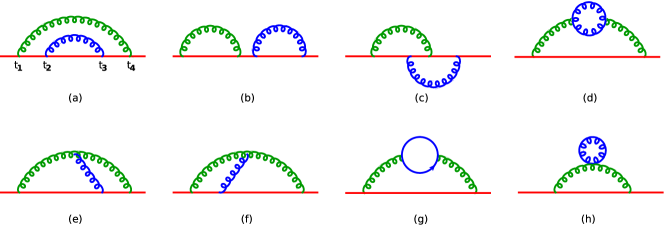
Figure 1: Forward scattering amplitudes at $O(\alpha_{s}^{2})$. All the relevant graphs for calculating the energy loss due to two-gluon emission can be obtained by cutting through these amplitudes.

In this subsection we give all the graphs for the energy loss due to two-gluon emission, which is denoted by $\Delta E_{2}$. In these graphs at least one of the two gluons is real. In terms of the spectra defined in the previous subsection, $\Delta E_{2}$ is given by

$$\Delta E_{2}=\int d\omega_{1}d\omega_{2}\left(\omega_{1}+\omega_{2}\right)\frac{dI^{(2,0)}}{d\omega_{1}d\omega_{2}}+\int d\omega_{1}d\omega_{2}\omega_{1}\frac{dI^{(1,1)}}{d\omega_{1}d\omega_{2}}.$$ (14)

All the graphs contributing to $\Delta E_{2}$ can be obtained by cutting through the forward amplitudes in Fig. 1. The cuts of Fig. 1 (h) are not relevant for medium-induced energy loss and shall be ignored. Besides, we shall also ignore the graphs obtained by cutting Fig. 1 (g) because the gluon-quark transition is suppressed compared to the soft gluon emission at high energies. Then, we are left with 17 possible cuts of Fig. 1 (a) to (f).

Even in the same graph, different orderings in the 4 emission (absorption) times of the two gluons give different contributions, which need to be dealt with separately. The complete calculate of $\Delta E_{2}$ involves all the possible orderings in these 4 time variables. The graph with one of such orderings is referred to as a diagram in this paper. It is easy to show that there are a total of $78$ different diagrams, which can be classified as follows

• 12 uncorrelated emissions:
  In these diagrams both of the two emission times of one gluon are later than those of the other. The distribution of the uncorrelated soft gluons is the QCD analog of that of the soft photons in QED, which has the form of a Poisson distribution after all the uncorrelated multiple gluon emissions are includedBDMS:2001:uncorrelated . And there is no double logarithmic correction proportional to $\ln^{2}\left(\frac{L}{l_{0}}\right)^{2}$ from these diagrams.

• 26 fully-overlapping emissions:
  In these diagrams both of the two emission times of one gluon lie in between those of the other gluon. In the following sections we shall show that there is a double logarithmic correction to $\Delta E_{2}$ from these diagrams, which is the same as that to $\langle p_{\perp}^{2}\rangle$ in Ref. Liou:Mueller:Wu:2013 .

• 40 partially-overlapping emissions:
  In these diagrams only one of the two emission times of one gluon lies in between those of the other gluon. The evaluation of those diagrams is the most difficult part to obtain the complete result of $\Delta E_{2}$. Fortunately, unlike the fully-overlapping emissions the diagrams contributing to the double logarithmic terms $\propto\ln^{2}\frac{L}{l_{0}}$ of $\langle p_{\perp}^{2}\rangle$ do not show up as subdiagrams of these diagrams. Therefore, there is no double logarithmic correction the same as that in $\langle p_{\perp}^{2}\rangle$ from these diagrams.

III The time evolution of two gluons in the medium

Figure 2: Time-evolution of two gluons and a dipole in the medium. The first gluon with energy $\omega_{1}$ emitted off the quark at $t=z_{1}$ lives until $t=z_{4}$. The second gluon with energy $\omega_{2}$ is emitted at $t=z_{2}$ and absorbed at $t=z_{3}$ either by the first gluon or by the dipole. The transverse coordinates of the first and the second gluon are respectively denoted by ${\bf x}$ and ${\bf B}$, and the dipole locates at ${\bf{0}}$. Here, the time variables satisfy $0<z_{1}<z_{2}<z_{3}<z_{4}<L$.

In this paper we use a dipole-like picture to describe the whole process of two-gluon emission in the QCD mediumLiou:Mueller:Wu:2013 . In our calculation we shall only include the fully-overlapping emissions as illustrated in Fig. 2: the first gluon with energy $\omega_{1}$ emitted off the quark at $t=z_{1}$ lives until $t=z_{4}$; and the second gluon with energy $\omega_{2}$ is emitted at $t=z_{2}>z_{1}$ and absorbed at $t=z_{3}<z_{4}$ either by the first gluon or by the dipole. In our case the energy of the high-energy parton $E\gg\hat{q}L^{2}$ and, therefore, the change of the transverse coordinates of the dipole can be neglected. Due to the homogeneity of the medium in the transverse plane, our result should be independent of the transverse coordinates of the dipole, which are chozen to be ${\bf 0}$.

The time evolution of one gluon with energy $\omega_{1}$ together with the dipole inside the medium is described by $G^{(3)}$BDMPS:1996 ; BDMPS:1998 ; Zakharov:1996 ; Zakharov:1997

$$G^{(3)}({\bf B}_{2},z_{2},{\bf B}_{1},z_{1};\omega_{1})$$

$$\equiv\int\limits_{{\bf B}(z_{1})={\bf B}_{1}}^{{\bf B}(z_{2})={\bf B}_{2}}D{\bf B}\exp\left\{\int_{z_{1}}^{z_{2}}d\xi\left[i\frac{\omega_{1}}{2}\dot{{\bf B}}^{2}+\frac{N_{c}n(\xi)}{C_{R}}\left(\sigma_{R}({\bf B},\xi)-\sigma_{R}(0_{\perp},\xi)\right)\right]\right\}.$$ (15)

For the medium-induced energy loss the harmonic oscillator approximation is justifiedBDMPS:1996 and one has

$$G^{(3)}({\bf B}_{2},z_{2},{\bf B}_{1},z_{1};\omega)\simeq G({\bf B}_{2},{\bf B}_{1},z_{2}-z_{1};\omega_{1},\Omega_{1}),$$ (16)

where

$$\Omega_{j}=\frac{1-i}{2}\sqrt{\frac{\hat{q}_{A}}{\omega_{j}}}\qquad\text{ with }j=1,2\text{ and }\hat{q}_{A}\equiv\frac{N_{c}}{C_{R}}\hat{q},$$ (17)

and the propagator of the harmonic oscillator

$$G({\bf B}_{2},{\bf B}_{1},z,\omega,\Omega)\equiv\frac{\omega\Omega}{2\pi i\sin(\Omega z)}\exp\left\{\frac{i\omega\Omega}{2\sin(\Omega z)}\left[\left({\bf B}_{2}^{2}+{\bf B}_{1}^{2}\right)\cos(\Omega z)-2{\bf B}_{2}\cdot{\bf B}_{1}\right]\right\}.$$ (18)

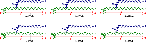
Figure 3: Scattering of two gluons and a dipole off one scatterer. All the possible hookings of the two gluon lines issued from the scatterer on the 4 partons are shown in this figure. In the cases when one gluon line of the scatterer is hooked either on the quark line or on the antiquark line of the dipole, the end of the gluon line is put in between the quark-antiquark pair. Here, $a,b,c$ and $d$ are color indices, ${\bf 0},{\bf x}$ and ${\bf B}$ are the transverse coordinates, and $\omega_{1}$ and $\omega_{2}$ are the energies of the two gluons.

During $z_{3}>t>z_{2}$ one needs to understand how the two gluons together with the dipole evolve in the medium. Fig. 3 shows all the possible diagrams for the scattering of the two gluons and the dipole off one scatterer. Without any scattering one has the color matrix $(T_{A}^{d})_{ce}T^{e}_{R}$ for the 4-body system. Including the scattering off one scatterer one has $\frac{N_{c}}{2}(T_{A}^{d})_{ce}T^{e}_{R}$ for each diagram in the figure, which gives the color factor $\frac{N_{c}}{2}$ for each diagram. As a result the potential of the evolution Hamiltonian of the 4-body system can be easily calculated, which takes the form

$$-iV^{(4)}(t,{\bf x},{\bf B})=\frac{N_{c}n(t)}{2C_{R}}\left[\sigma_{R}({\bf x})+\sigma_{R}({\bf B})+\sigma_{R}({\bf B}-{\bf x})-3\sigma_{R}({\bf 0})\right].$$ (19)

Let us assume that the first gluon is emitted off the quark of the dipole. If the second gluon is emitted off the first gluon or the quark, the propagator of the 4-body system is given by

$$G^{(4)}({\bf x}_{3},{\bf B}_{3},z_{3};{\bf x}_{2},{\bf B}_{2},z_{2};\omega_{1},\omega_{2})$$

$$\equiv\int\limits_{{\bf x}(z_{2})={\bf x}_{2},{\bf B}(z_{2})={\bf B}_{2}}^{{\bf x}(z_{3})={\bf x}_{3},{\bf B}(z_{3})={\bf B}_{3}}D{\bf x}D{\bf B}e^{i\int_{z_{1}}^{z_{2}}d\xi\left[\frac{1}{2}\omega_{1}\dot{{\bf x}}^{2}+\frac{1}{2}\omega_{2}\dot{{\bf B}}^{2}-V^{(4)}(\xi,{\bf x},{\bf B})\right]}.$$ (20)

Otherwise, the propagator takes the form

$$\bar{G}^{(4)}({\bf x}_{3},{\bf B}_{3},z_{3};{\bf x}_{2},{\bf B}_{2},z_{2};\omega_{1},\omega_{2})$$

$$\equiv\int\limits_{{\bf x}(z_{2})={\bf x}_{2},{\bf B}(z_{2})={\bf B}_{2}}^{{\bf x}(z_{3})={\bf x}_{3},{\bf B}(z_{3})={\bf B}_{3}}D{\bf x}D{\bf B}e^{i\int_{z_{1}}^{z_{2}}d\xi\left[\frac{1}{2}\omega_{1}\dot{{\bf x}}^{2}-\frac{1}{2}\omega_{2}\dot{{\bf B}}^{2}-V^{(4)}(\xi,{\bf x},{\bf B})\right]}$$

$$=G^{(4)}({\bf x}_{3},{\bf B}_{3},z_{3};{\bf x}_{2},{\bf B}_{2},z_{2};\omega_{1},-\omega_{2}).$$ (21)

In the harmonic oscillator approximation one has

$$G^{(4)}({\bf x}_{3},{\bf B}_{3},z_{3};{\bf x}_{2},{\bf B}_{2},z_{2};\omega_{1},\omega_{2})$$

$$\simeq\int\limits_{{\bf x}(z_{2})={\bf x}_{2},{\bf B}(z_{2})={\bf B}_{2}}^{{\bf x}(z_{3})={\bf x}_{3},{\bf B}(z_{3})={\bf B}_{3}}D{\bf x}D{\bf B}e^{\int_{z_{1}}^{z_{2}}d\xi\left\{\frac{i}{2}\omega_{1}\dot{{\bf x}}^{2}+\frac{i}{2}\omega_{2}\dot{{\bf B}}^{2}-\frac{\hat{q}_{A}}{8}\left[{\bf x}^{2}+{\bf B}^{2}+({\bf B}-{\bf x})^{2}\right]\right\}}$$

$$=G(\tilde{{\bf x}}_{3},\tilde{{\bf x}}_{2},z_{3}-z_{2},m_{1},K_{1})G(\tilde{{\bf B}}_{3},\tilde{{\bf B}}_{2},z_{3}-z_{2},m_{2},K_{2}),$$ (22)

where the new coordinates are defined as

$$\left(\begin{array}[]{c}\tilde{{\bf x}}\\ \tilde{{\bf B}}\end{array}\right)=\left(\begin{array}[]{cc}1&\frac{-\omega_{1}+\omega_{2}+\sqrt{\omega_{1}^{2}-\omega_{1}\omega_{2}+\omega_{2}^{2}}}{\omega_{1}}\\ -\frac{1}{2}&\frac{\omega_{1}-\omega_{2}+\sqrt{\omega_{1}^{2}-\omega_{1}\omega_{2}+\omega_{2}^{2}}}{2\omega_{1}}\\ \end{array}\right)\left(\begin{array}[]{c}{\bf x}\\ {\bf B}\end{array}\right),$$ (29)

and

$$m_{1}=\frac{\omega_{1}\left(\omega_{1}-\omega_{2}+\sqrt{\omega_{1}^{2}-\omega_{1}\omega_{2}+\omega_{2}^{2}}\right)}{2\sqrt{\omega_{1}^{2}-\omega_{2}\omega_{1}+\omega_{2}^{2}}},$$ (30)

$$m_{2}=\frac{2\omega_{1}\left(\omega_{2}-\omega_{1}+\sqrt{\omega_{1}^{2}-\omega_{1}\omega_{2}+\omega_{2}^{2}}\right)}{\sqrt{\omega_{1}^{2}-\omega_{2}\omega_{1}+\omega_{2}^{2}}},$$ (31)

$$K_{1}^{2}=-\frac{i\hat{q}_{A}\left(\omega_{1}+\omega_{2}-\sqrt{\omega_{1}^{2}-\omega_{1}\omega_{2}+\omega_{2}^{2}}\right)}{4\omega_{1}\omega_{2}},$$ (32)

$$K_{2}^{2}=-\frac{i\hat{q}_{A}\left(\omega_{1}+\omega_{2}+\sqrt{\omega_{1}^{2}-\omega_{1}\omega_{2}+\omega_{2}^{2}}\right)}{4\omega_{1}\omega_{2}}.$$ (33)

In the case $\omega_{1}\gg\omega_{2}$ one has

$$G^{(4)} ({\bf x}_{3},{\bf B}_{3},z_{3};{\bf x}_{2},{\bf B}_{2},z_{2};\omega_{1},\omega_{2})$$ (34)

$$\simeq G({\bf x}_{3},{\bf x}_{2},z_{3}-z_{2},\omega_{1},\frac{\sqrt{3}}{2}\Omega_{1})G(\bar{{\bf B}}_{3},\bar{{\bf B}}_{2},z_{3}-z_{2},\omega_{2},\Omega_{2}),$$

$$\bar{G}^{(4)} ({\bf x}_{3},{\bf B}_{3},z_{3};{\bf x}_{2},{\bf B}_{2},z_{2};\omega_{1},\omega_{2})$$ (35)

$$\simeq G({\bf x}_{3},{\bf x}_{2},z_{3}-z_{2},\omega_{1},\frac{\sqrt{3}}{2}\Omega_{1})G^{*}(\bar{{\bf B}}_{3},\bar{{\bf B}}_{2},z_{3}-z_{2},\omega_{2},\Omega_{2}),$$

where

$$\bar{{\bf B}}_{2}\equiv{\bf B}_{2}-\frac{{\bf x}_{2}}{2},\qquad\text{and}\qquad\bar{{\bf B}}_{3}\equiv{\bf B}_{3}-\frac{{\bf x}_{3}}{2}.$$ (36)

IV The double logarithmic correction to radiative energy loss

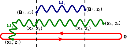
Figure 4: Diagrams with fully-overlapping emissions. 13 diagrams can be constructed from this figure as follows. If the first gluon with energy $\omega_{1}$ is absorbed by the antiquark at $t=z_{4}$, the ends of the second gluon line with energy $\omega_{2}$ can be attached to the first gluon line or the diplole in 9 different ways. In contrast, the ends of the second gluon line can be attached to the first gluon line or the dipole in 4 different ways if the first gluon is absorbed by the quark. These 13 diagrams and their complex conjugates all contribute to $\Delta E_{2}$.

In this section we calculate the double logarithmic correction to radiative energy loss. The double logarithmic correction comes from the diagrams with fully-overlapping emission defined in Sec. II. All these diagrams can be constructed either from Fig. 4 or its complex conjugate. First, we give all the contributions of these diagrams to $\Delta E_{2}$ in a compact form in terms of $G^{(3)}$ and $G^{(4)}$ ($\bar{G}^{(4)}$) defined in the previous section. Next, we shall show that they give a double logarithmic correction to radiative energy loss, which is the same as that to the radiative $p_{\perp}$-broadening in Ref. Liou:Mueller:Wu:2013 .

IV.1 Contributions from diagrams with fully-overlapping emission

In total, there are 26 diagrams with fully-overlapping emission. Let us denote the energies of the two gluons respectively by $\omega_{1}$ and $\omega_{2}$ and their formation times respectively by $t_{1}\equiv z_{4}-z_{1}$ and $t_{2}\equiv z_{3}-z_{2}$. And we assume that $\omega_{1}\gtrsim\omega_{2}$ and $t_{1}\gtrsim t_{2}$. As illustrated in Fig. 4, there are respectively 4 or 9 diagrams in which the gluon with energy $\omega_{1}$ is virtual or real. The 26 fully-overlapping emissions include these 13 diagrams and their complex conjugates. And one can obtain the corrections to the energy loss from fully-overlapping emissions by taking 2 times the real part of the contributions of these 13 diagrams.

There are some cancellations between the contributions from different diagrams. As a consequence of the conservation of probability, moving one gluon emission (absorption) vertex from the quark (antiquark) line to the antiquark (quark) line in a diagram only changes the overall sign of the contribution of the diagramWu:2011 . To see such a cancellation easily, we use a diagramatic representation in which the integrations over all the time variables and transverse coordinates in Fig. 4 are omitted. It is easy to see that we have the following cancellation

$$I_{a}=\int d\omega_{1}d\omega_{2} \left\{\left[\left(\omega_{1}+\omega_{2}\right)\left(\begin{array}[]{c}\includegraphics[width=56.9055pt]{f04}\end{array}\right)+\omega_{2}\left(\begin{array}[]{c}\includegraphics[width=56.9055pt]{f04c}\end{array}\right)\right]\right.$$ (48)

$$+\left[\left(\omega_{1}+\omega_{2}\right)\left(\begin{array}[]{c}\includegraphics[width=56.9055pt]{f05}\end{array}\right)+\omega_{2}\left(\begin{array}[]{c}\includegraphics[width=56.9055pt]{f05c}\end{array}\right)\right]$$

$$+\left[\left(\omega_{1}+\omega_{2}\right)\left(\begin{array}[]{c}\includegraphics[width=56.9055pt]{f08}\end{array}\right)+\omega_{2}\left(\begin{array}[]{c}\includegraphics[width=56.9055pt]{f08c}\end{array}\right)\right]$$

$$+\left.\left[\left(\omega_{1}+\omega_{2}\right)\left(\begin{array}[]{c}\includegraphics[width=56.9055pt]{f09}\end{array}\right)+\omega_{2}\left(\begin{array}[]{c}\includegraphics[width=56.9055pt]{f09c}\end{array}\right)\right]\right\}$$

$$=\int d\omega_{1}d\omega_{2} ~{}\omega_{1}~{}\left\{\left(\begin{array}[]{c}\includegraphics[width=56.9055pt]{f04}\end{array}\right)+\left(\begin{array}[]{c}\includegraphics[width=56.9055pt]{f05}\end{array}\right)\right.$$ (54)

$$+\left.\left(\begin{array}[]{c}\includegraphics[width=56.9055pt]{f08}\end{array}\right)+\left(\begin{array}[]{c}\includegraphics[width=56.9055pt]{f09}\end{array}\right)\right\}.$$

Therefore, only these 9 diagrams with the gluon of energy $\omega_{1}$ being real contribute to $\Delta E_{2}$.

The contributions to $\Delta E_{2}$ from these 9 diagrams and their complex conjugates can be classified as follows

$$e_{1}\equiv \frac{2}{(4\pi)^{2}}\text{Re}\int d\omega_{1}d\omega_{2}\omega_{1}\left[\left(\begin{array}[]{c}\includegraphics[width=56.9055pt]{f01}\end{array}\right)+\left(\begin{array}[]{c}\includegraphics[width=56.9055pt]{f04}\end{array}\right)+\left(\begin{array}[]{c}\includegraphics[width=56.9055pt]{f06}\end{array}\right)\right],$$ (58)

$$e_{2}\equiv \frac{2}{(4\pi)^{2}}\text{Re}\int d\omega_{1}d\omega_{2}\omega_{1}\left[\left(\begin{array}[]{c}\includegraphics[width=56.9055pt]{f07}\end{array}\right)+\left(\begin{array}[]{c}\includegraphics[width=56.9055pt]{f08}\end{array}\right)+\left(\begin{array}[]{c}\includegraphics[width=56.9055pt]{f02}\end{array}\right)\right],$$ (62)

$$e_{3}\equiv \frac{2}{(4\pi)^{2}}\text{Re}\int d\omega_{1}d\omega_{2}\omega_{1}\left[\left(\begin{array}[]{c}\includegraphics[width=56.9055pt]{f05}\end{array}\right)+\left(\begin{array}[]{c}\includegraphics[width=56.9055pt]{f03}\end{array}\right)+\left(\begin{array}[]{c}\includegraphics[width=56.9055pt]{f09}\end{array}\right)\right].$$ (66)

It is easy to show that the overall color factors for $e_{1},e_{2}$ and $e_{3}$ are respectively given by $N_{c}C_{R}$, $N_{c}C_{R}/2$ and $N_{c}C_{R}/2$. In terms of $G^{(3)}$, $G^{(4)}$ and $\bar{G}^{(4)}$, we get, from the Feynman rules in Sec. II, the following compact expressions

$$e_{1}=2\alpha_{s}^{2}N_{c}C_{R}~{}\text{Re} ~{}\iiint\triangledown_{{\bf x}_{1}}\cdot\left.\triangledown_{{\bf x}_{4}}\left[G^{(3)}({\bf x}_{4},z_{4},{\bf x}_{3},z_{3};\omega_{1})G^{(3)}({\bf x}_{2},z_{2};{\bf x}_{1},z_{1};\omega_{1})\right]\right|^{{\bf x}_{1}=0={\bf x}_{4}}$$ (67)

$$\times\triangledown_{{\bf B}_{2}}\cdot\left.\triangledown_{{\bf B}_{3}}G^{(4)}({\bf x}_{3},{\bf B}_{3},z_{3};{\bf x}_{2},{\bf B}_{2},z_{2};\omega_{1},\omega_{2})\right|^{{\bf B}_{2}={\bf x}_{2},{\bf B}_{3}=0}_{{\bf B}_{2}={\bf x}_{2},{\bf B}_{3}={\bf x}_{3}},$$

$$e_{2}=\alpha_{s}^{2}N_{c}C_{R}~{}\text{Re}~{} \iiint\triangledown_{{\bf x}_{1}}\cdot\left.\triangledown_{{\bf x}_{4}}\left[G^{(3)}({\bf x}_{4},z_{4},{\bf x}_{3},z_{3};\omega_{1})G^{(3)}({\bf x}_{2},z_{2};{\bf x}_{1},z_{1};\omega_{1})\right]\right|^{{\bf x}_{1}=0={\bf x}_{4}}$$ (68)

$$\times\triangledown_{{\bf B}_{2}}\cdot\left.\triangledown_{{\bf B}_{3}}G^{(4)}({\bf x}_{3},{\bf B}_{3},z_{3};{\bf x}_{2},{\bf B}_{2},z_{2};\omega_{1},\omega_{2})\right|^{{\bf B}_{2}=0,{\bf B}_{3}={\bf x}_{3}}_{{\bf B}_{2}=0,{\bf B}_{3}=0},$$

$$e_{3}=\alpha_{s}^{2}N_{c}C_{R}~{}\text{Re}~{} \iiint\triangledown_{{\bf x}_{1}}\cdot\left.\triangledown_{{\bf x}_{4}}\left[G^{(3)}({\bf x}_{4},z_{4},{\bf x}_{3},z_{3};\omega_{1})G^{(3)}({\bf x}_{2},z_{2};{\bf x}_{1},z_{1};\omega_{1})\right]\right|^{{\bf x}_{1}=0={\bf x}_{4}}$$ (69)

$$\times\triangledown_{{\bf B}_{2}}\cdot\left.\triangledown_{{\bf B}_{3}}\bar{G}^{(4)}({\bf x}_{3},{\bf B}_{3},z_{3};{\bf x}_{2},{\bf B}_{2},z_{2};\omega_{1},\omega_{2})\right|^{{\bf B}_{2}=0,{\bf B}_{3}={\bf x}_{3}}_{{\bf B}_{2}=0,{\bf B}_{3}=0},$$

where the short-hand notation

$$\iiint\equiv\int\frac{d\omega_{1}}{\omega_{1}^{2}}\frac{d\omega_{2}}{\omega_{2}^{3}}\int_{0}^{L}dz_{4}\int_{0}^{z_{4}}dz_{3}\int_{0}^{z_{3}}dz_{2}\int_{0}^{z_{2}}dz_{1}\int d^{2}{\bf x}_{2}d^{2}{\bf x}_{3}.$$ (70)

And the contributions from all the fully-overlapping emissions to the energy loss are given by

$$\Delta E_{2}= e_{1}+e_{2}+e_{3}.$$ (71)

It is still too complicated to be evaluated analytically even in the harmonic oscillator approximation. In the next subsection, we shall evaluate it in the double logarithmic approximation following Ref. Liou:Mueller:Wu:2013 .

IV.2 $\Delta E_{2}$ in the double logarithmic approximation

The calculation of $\Delta E_{2}$ in eq. (71) is simplified in the double logarithmic region. The first gluon with energy $\omega_{1}$, similar to that in the case with one-gluon emission, typically has $t_{1}\equiv z_{4}-z_{1}\simeq L$, $\omega_{1}\simeq\hat{q}L^{2}$ and $|{\bf x}|^{2}\simeq\frac{1}{\hat{q}L}$. In the double logarithmic regionLiou:Mueller:Wu:2013 , the second gluon with energy $\omega_{2}$ typically has

$$|{\bf B}|^{2}\gtrsim|{\bf x}|^{2},\qquad\omega_{2}\lesssim\omega_{1},\qquad\text{and}\qquad t_{2}\lesssim\sqrt{\frac{\omega_{2}}{\hat{q}_{A}}}\lesssim\sqrt{\frac{\omega_{1}}{\hat{q}_{A}}}\simeq t_{1}.$$ (72)

In this region one can use the following approximation

$$G^{(4)}({\bf x}_{3},{\bf B}_{3},z_{3};{\bf x}_{2},{\bf B}_{2},z_{2};\omega_{1},\omega_{2})\simeq\delta({\bf x}_{3}-{\bf x}_{2})e^{-\frac{3}{16}\hat{q}_{A}x_{2}^{2}t_{2}}G(\bar{\bf B}_{3},\bar{\bf B}_{2},t_{2},\omega_{2},\Omega_{2}),$$ (73)

$$\bar{G}^{(4)}({\bf x}_{3},{\bf B}_{3},z_{3};{\bf x}_{2},{\bf B}_{2},z_{2};\omega_{1},\omega_{2})\simeq\delta({\bf x}_{3}-{\bf x}_{2})e^{-\frac{3}{16}\hat{q}_{A}x_{2}^{2}t_{2}}G^{*}(\bar{\bf B}_{3},\bar{\bf B}_{2},t_{2},\omega_{2},\Omega_{2}).$$ (74)

By inserting (16), (73) and (74) into (71), we have

$$\Delta E_{2}\simeq 2\alpha_{s}^{2}N_{c}C_{R}\int\frac{d\omega_{1}}{\omega_{1}^{2}}\frac{d\omega_{2}}{\omega_{2}^{3}}\int_{0}^{L}dz_{4}\int_{0}^{L-z_{4}}dz_{1}\int_{z_{1}}^{z_{4}}dz_{3}\int_{0}^{z_{3}-z_{1}}dt_{2}\int d^{2}{\bf x}_{2}e^{-\frac{3}{16}\hat{q}_{A}x_{2}^{2}t_{2}}$$ (75)

$$\times\text{Re}\left\{\triangledown_{{\bf x}_{1}}\cdot\left.\triangledown_{{\bf x}_{4}}\left[G({\bf x}_{4},{\bf x}_{2},z_{4}-z_{3};\omega_{1},\Omega_{1})G({\bf x}_{2},{\bf x}_{1},z_{3}-t_{2}-z_{1};\omega_{1},\Omega_{1})\right]\right|^{{\bf x}_{1}=0={\bf x}_{4}}\right.$$

$$\times\left.\left[\triangledown_{{\bf B}_{2}}\cdot\left.\triangledown_{{\bf B}_{3}}G({\bf B}_{3}-\frac{{\bf x}_{2}}{2},{\bf B}_{2}-\frac{{\bf x}_{2}}{2},t_{2};\omega_{2},\Omega_{2})\right|^{{\bf B}_{2}={\bf x}_{2},{\bf B}_{3}=0}_{{\bf B}_{2}={\bf x}_{2},{\bf B}_{3}={\bf x}_{2}}\right.\right.$$

$$+\left.\left.\text{Re}\triangledown_{{\bf B}_{2}}\cdot\left.\triangledown_{{\bf B}_{3}}G({\bf B}_{3}-\frac{{\bf x}_{2}}{2},{\bf B}_{2}-\frac{{\bf x}_{2}}{2},t_{2};\omega_{2},\Omega_{2})\right|^{{\bf B}_{2}=0,{\bf B}_{3}={\bf x}_{2}}_{{\bf B}_{2}=0,{\bf B}_{3}=0}\right]\right\}.$$

In the double logarithmic region one has $t_{1}\lesssim t_{2}$. Therefore, we can neglect the difference between $z_{3}$ and $z_{2}$ and write

$$\Delta E_{2}\simeq 2\alpha_{s}N_{c}\int\frac{d\omega_{1}}{\omega_{1}^{2}}\int_{0}^{L}dz_{4}\int_{0}^{L-z_{4}}dz_{1}\int_{z_{1}}^{z_{4}}dz_{3}\int d^{2}{\bf x}_{2}\text{Re}\left\{S({\bf x}_{2},z_{3}-z_{1})\right.$$ (76)

$$\times\left.\left.\triangledown_{{\bf x}_{1}}\cdot\triangledown_{{\bf x}_{4}}\left[G({\bf x}_{4},{\bf x}_{2},z_{4}-z_{3};\omega_{1},\Omega_{1})G({\bf x}_{2},{\bf x}_{1},z_{3}-z_{1};\omega_{1},\Omega_{1})\right]\right|^{{\bf x}_{1}=0={\bf x}_{4}}\right\},$$

where

$$S({\bf x}_{2}, z_{3}-z_{1})\equiv\alpha_{s}C_{R}\int\frac{d\omega_{2}}{\omega_{2}^{3}}\int_{0}^{z_{3}-z_{1}}dt_{2}e^{-\frac{3}{16}\hat{q}_{A}x_{2}^{2}t_{2}}$$ (77)

$$\times\left.\left[\triangledown_{{\bf B}_{2}}\cdot\left.\triangledown_{{\bf B}_{3}}G({\bf B}_{3}-\frac{{\bf x}_{2}}{2},{\bf B}_{2}-\frac{{\bf x}_{2}}{2},t_{2};\omega_{2},\Omega_{2})\right|^{{\bf B}_{2}={\bf x}_{2},{\bf B}_{3}=0}_{{\bf B}_{2}={\bf x}_{2},{\bf B}_{3}={\bf x}_{2}}\right.\right.$$

$$+\left.\text{Re}\triangledown_{{\bf B}_{2}}\cdot\left.\triangledown_{{\bf B}_{3}}G({\bf B}_{3}-\frac{{\bf x}_{2}}{2},{\bf B}_{2}-\frac{{\bf x}_{2}}{2},t_{2};\omega_{2},\Omega_{2})\right|^{{\bf B}_{2}=0,{\bf B}_{3}={\bf x}_{2}}_{{\bf B}_{2}=0,{\bf B}_{3}=0}\right].$$

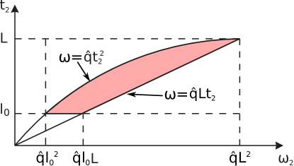
Figure 5: Kinetic region for double logarithmic correctionLiou:Mueller:Wu:2013 . The double logarithmic region is enclosed by the following three curves: $t_{2}=l_{0}$, $\omega_{2}=\hat{q}Lt_{2}$ and $\omega_{2}=\hat{q}t_{2}^{2}$.

Now we are ready to show how the double logarithmic correction to radiative $p_{\perp}$-broadening shows up in the calculation of radiative energy loss. By dropping terms independent of $\hat{q}$ and keeping only the double logarithmic terms proportional to $x_{2}^{2}$, we have

$$S({\bf x}_{2}, z_{3}-z_{1})\simeq-\frac{\alpha_{s}N_{c}}{4\pi}\hat{q}x_{2}^{2}\int\frac{d\omega_{2}}{\omega_{2}}\int_{0}^{z_{3}-z_{1}}\frac{dt_{2}}{t_{2}}=-\frac{\alpha_{s}N_{c}}{32\pi}\hat{q}x_{2}^{2}\ln^{2}\left(\frac{z_{3}-z_{1}}{l_{0}}\right)^{2},$$ (78)

where $t_{2}$ and $\omega_{2}$ have been integrated over the double logarithmic region in Fig. 5 with $L$ replaced by $z_{3}-z_{1}$. As we shall show below, one can simply replace $z_{3}-z_{1}$ in (78) by $L$ in the double logarithmic approximation. Therefore, such a double logarithmic result is exactly the same as that of radiative $\langle p_{\perp}^{2}\rangle$ and eq. (78) is the same as eq. (26) in Ref. Liou:Mueller:Wu:2013 divided by $L$.

Let us evaluate the double logarithmic correction to radiative energy loss. Inserting (78) into (76) and integrating out $x_{2}$ gives

$$\Delta E_{2}\simeq \frac{\alpha_{s}^{2}N_{c}^{2}}{4\pi^{2}}\hat{q}\text{Re}~{}i\int\frac{d\omega_{1}}{\omega_{1}}\int_{0}^{L}dz_{4}\int_{0}^{L-z_{4}}dz_{1}$$ (79)

$$\times\int_{z_{1}}^{z_{4}}dz_{3}\ln^{2}\left(\frac{z_{3}-z_{1}}{l_{0}}\right)^{2}\frac{\Omega_{1}\sin(\Omega_{1}(z_{4}-z_{3}))\sin(\Omega_{1}(z_{3}-z_{1}))}{\sin^{3}(\Omega_{1}(z_{4}-z_{1}))}.$$

Since the integrand on the right-hand side of the above equation is proportional to $z_{3}-z_{1}$ as $z_{3}\to z_{1}$, the leading double logarithmic term from the integration over $z_{3}$ can be obtained simply by integration by parts, that is,

$$\Delta E_{2}\simeq \frac{\alpha_{s}^{2}N_{c}^{2}}{4\pi^{2}}\hat{q}\text{Re}~{}i\int\frac{d\omega_{1}}{\omega_{1}}\int_{0}^{L}dz_{4}\int_{0}^{L-z_{4}}dz_{1}\ln^{2}\left(\frac{z_{4}-z_{1}}{l_{0}}\right)^{2}$$

$$\times\int_{z_{1}}^{z_{4}}dz_{3}\frac{\Omega_{1}\sin(\Omega_{1}(z_{4}-z_{3}))\sin(\Omega_{1}(z_{3}-z_{1}))}{\sin^{3}(\Omega_{1}(z_{4}-z_{1}))}$$

$$= \frac{\alpha_{s}^{2}N_{c}^{2}}{8\pi^{2}}\hat{q}\text{Re}~{}i\int\frac{d\omega_{1}}{\omega_{1}}\int_{0}^{L}dt_{1}(L-t_{1})\ln^{2}\left(\frac{t_{1}}{l_{0}}\right)^{2}\frac{\Omega_{1}\sin(\Omega_{1}t_{1})-\Omega_{1}t_{1}\cos(\Omega_{1}t_{1})}{\sin^{3}(\Omega_{1}t_{1})}.$$ (80)

Similarly, the leading double logarithmic term from the integration over $t_{1}$ is of the form

$$\Delta E_{2}\simeq \frac{\alpha_{s}^{2}N_{c}^{2}}{8\pi^{2}}\hat{q}\ln^{2}\left(\frac{L}{l_{0}}\right)^{2}\text{Re}~{}i\int_{0}^{\infty}\frac{d\omega_{1}}{\omega_{1}}\int_{0}^{L}dt_{1}(L-t_{1})\frac{\Omega_{1}\sin(\Omega_{1}t_{1})-\Omega_{1}t_{1}\cos(\Omega_{1}t_{1})}{\sin^{3}(\Omega_{1}t_{1})}$$

$$= \frac{\alpha_{s}^{2}N_{c}^{2}}{16\pi^{2}}\hat{q}\ln^{2}\left(\frac{L}{l_{0}}\right)^{2}\text{Re}~{}i\int_{0}^{\infty}\frac{d\omega_{1}}{\omega_{1}}\frac{1}{\Omega_{1}^{2}}\left(1-\frac{\Omega_{1}L}{\tan(\Omega_{1}L)}\right)$$

$$= \frac{\alpha_{s}^{2}N_{c}^{2}}{16\pi^{2}}\hat{q}L^{2}\ln^{2}\left(\frac{L}{l_{0}}\right)^{2}\text{Re}\int_{0}^{\infty}\frac{d\hat{\omega}}{\hat{\omega}^{3}}\left(\frac{(1-i)\hat{\omega}}{\tan((1-i)\hat{\omega})}-1\right)$$

$$= \frac{\alpha_{s}N_{c}}{12}L\times\frac{\alpha_{s}N_{c}}{8\pi}\hat{q}\ln^{2}\left(\frac{L}{l_{0}}\right)^{2}L=\frac{\alpha_{s}N_{c}}{12}L\langle p_{\perp}^{2}\rangle_{rad},$$ (81)

where $\hat{\omega}\equiv\frac{1}{2}\sqrt{\frac{\hat{q}_{A}L^{2}}{\omega}}$ and recall that radiative energy loss due to one-gluon emission is given byBDMPS:1998

$$\Delta E_{1}= 2\alpha_{s}C_{R}\text{Re}\int\frac{d\omega_{1}}{\omega_{1}^{2}}\int_{0}^{L}dt(L-t)\triangledown_{{\bf x}_{1}}\cdot\triangledown_{{\bf x}_{4}}\left.\left[G({\bf x}_{4},{\bf x}_{1},t;\omega_{1},\Omega_{1})\right.\right.$$ (82)

$$\left.\left.-G({\bf x}_{4},{\bf x}_{1},t;\omega_{1},0)\right]\right|^{{\bf x}_{1}=0={\bf x}_{4}}=\frac{\alpha_{s}N_{c}}{12}\hat{q}L^{2}.$$

The resummation of the double logarithmic correction in eq. (IV.2) can be carried out in exactly the same way as that in the calculation of $\langle p_{\perp}^{2}\rangle$. For $(n+1)$-gluon emission, one has

$$S({\bf x}_{2}, z_{3}-z_{1})\simeq-\frac{1}{4}\hat{q}x_{2}^{2}\frac{1}{n!(n+1)!}\left[\frac{\alpha_{s}N_{c}}{4\pi}\ln^{2}\left(\frac{z_{3}-z_{1}}{l_{0}}\right)^{2}\right]^{n},$$ (83)

which gives

$$\Delta E_{n+1}= \frac{\alpha_{s}N_{c}}{12}L\frac{\hat{q}L}{n!(n+1)!}\left[\frac{\alpha_{s}N_{c}}{4\pi}\ln^{2}\frac{L^{2}}{l_{0}^{2}}\right]^{n}.$$ (84)

Therefore, the total energy loss is given by

$$\Delta E=\sum\limits_{n=0}^{\infty}\Delta E_{n+1}=\frac{\alpha_{s}N_{c}}{12}L\frac{\hat{q}L}{\sqrt{\frac{\alpha_{s}N_{c}}{4\pi}}\ln\frac{L^{2}}{l_{0}^{2}}}I_{1}\left[\sqrt{\frac{\alpha_{s}N_{c}}{\pi}}\ln\frac{L^{2}}{l_{0}^{2}}\right]=\frac{\alpha_{s}N_{c}}{12}L\langle p_{\perp}^{2}\rangle.$$ (85)

V Conclusions

In this paper we calculate the double logarithmic correction to radiative energy loss of a high-energy parton in the generalized BMDMPS-Z formalismWu:2011 ; Liou:Mueller:Wu:2013 . Radiative energy loss per unit length due to one-gluon emission is given byBDMPS:1998

$$-\frac{dE_{1}}{dz}=\frac{\alpha_{s}N_{c}}{12}\hat{q}L.$$ (86)

In this case it is dominated by radiating one gluon with the maximum energy $\omega_{c}\simeq\hat{q}L^{2}$ and the formation time $t_{c}\simeq L$. And within $t_{c}$ the gluon is of a typical size $x^{2}\sim\frac{1}{\hat{q}L}$. The double logarithmic correction comes from the diagrams by adding a second gluon with the two emission times both lie in between those of the first gluon of energy $\omega_{c}$. In the kinetic region for the double logarithmic correction this second gluon has a smaller energy, a shorter formation time and a larger size than the first gluon. It modifies the transverse momentum broadening of the first gluon and, therefore, contributes to the radiative energy loss according to the parametric estimate in eq. (1). Our detailed calculation confirms this picture and we find that the double logarithmic correction to the energy loss due to two-gluon emission satisfies

$$-\frac{dE_{2}}{dz}=\frac{\alpha_{s}N_{c}}{12}\langle p_{\perp}^{2}\rangle_{rad},$$ (87)

where $\langle p_{\perp}^{2}\rangle_{rad}$ is given in eq. (3), which is obtained in Ref. Liou:Mueller:Wu:2013 . Moreover, the resummation of the double logarithmic terms can be carried out to give

$$-\frac{dE}{dz}=\frac{\alpha_{s}N_{c}}{12}\langle p_{\perp}^{2}\rangle,$$ (88)

where $\langle p_{\perp}^{2}\rangle$ is given in eq. (4). Our result agrees with that by using the renormalized $\hat{q}$ in Refs. Blaizot:Mehtar-Tani:2014 ; Iancu:2014 .

References

- (1) S. S. Adler et al. [PHENIX Collaboration], Phys. Rev. Lett. 91, 072301 (2003) [nucl-ex/0304022].
- (2) J. Adams et al. [STAR Collaboration], Phys. Rev. Lett. 91, 172302 (2003) [nucl-ex/0305015].
- (3) K. Aamodt et al. [ALICE Collaboration], Phys. Lett. B 696, 30 (2011) [arXiv:1012.1004 [nucl-ex]].
- (4) S. Chatrchyan et al. [CMS Collaboration], Eur. Phys. J. C 72, 1945 (2012) [arXiv:1202.2554 [nucl-ex]].
- (5) G. Aad et al. [ATLAS Collaboration], Phys. Lett. B 719, 220 (2013) [arXiv:1208.1967 [hep-ex]].
- (6) B. Muller, J. Schukraft and B. Wyslouch, Ann. Rev. Nucl. Part. Sci. 62, 361 (2012) [arXiv:1202.3233 [hep-ex]].
- (7) R. Baier, Y. L. Dokshitzer, A. H. Mueller, S. Peigne and D. Schiff, Nucl. Phys. B 484, 265 (1997) [hep-ph/9608322].
- (8) R. Baier, Y. L. Dokshitzer, A. H. Mueller, S. Peigne and D. Schiff, Nucl. Phys. B 483, 291 (1997) [arXiv:hep-ph/9607355].
- (9) R. Baier, Y. L. Dokshitzer, A. H. Mueller and D. Schiff, Nucl. Phys. B 531, 403 (1998) [arXiv:hep-ph/9804212].
- (10) B. Wu, JHEP 1110, 029 (2011) [arXiv:1102.0388 [hep-ph]].
- (11) T. Liou, A. H. Mueller and B. Wu, Nucl. Phys. A 916, 102 (2013) [arXiv:1304.7677 [hep-ph]].
- (12) M. Panero, K. Rummukainen and A. Schäfer, Phys. Rev. Lett. 112, 162001 (2014) [arXiv:1307.5850 [hep-ph]].
- (13) J. Casalderrey-Solana and X. N. Wang, Phys. Rev. C 77, 024902 (2008) [arXiv:0705.1352 [hep-ph]].
- (14) H. Xing, Z. B. Kang, E. Wang and X. N. Wang, arXiv:1407.8506 [hep-ph].
- (15) J. -P. Blaizot and Y. Mehtar-Tani, arXiv:1403.2323 [hep-ph].
- (16) E. Iancu, arXiv:1403.1996 [hep-ph].
- (17) B. G. Zakharov, JETP Lett. 63 (1996) 952 [arXiv:hep-ph/9607440].
- (18) B. G. Zakharov, JETP Lett. 65 (1997) 615 [arXiv:hep-ph/9704255].
- (19) A. Kovner and U. A. Wiedemann, In *Hwa, R.C. (ed.) et al.: Quark gluon plasma* 192-248 [hep-ph/0304151].
- (20) A. Majumder, arXiv:1405.2019 [nucl-th].
- (21) R. Baier, Y. L. Dokshitzer, A. H. Mueller and D. Schiff, JHEP 0109, 033 (2001) [hep-ph/0106347].
- (22) E. Iancu and D. N. Triantafyllopoulos, arXiv:1405.3525 [hep-ph].