Stretchy Polynomial Regression

Abstract

This article proposes a novel solution for stretchy polynomial regression learning. The solution comes in primal and dual closed-forms similar to that of ridge regression. Essentially, the proposed solution stretches the covariance computation via a power term thereby compresses or amplifies the estimation. Our experiments on both synthetic data and real-world data show effectiveness of the proposed method for compressive learning.

1 Introduction

The Weierstrass s approximation theory (see e.g., [1]) states that polynomials can approximate any continuous function on a closed and bounded interval to any degree of accuracy. This means that multivariate polynomials can provide an effective way to describe complex nonlinear input-output relationships [2].

However, on top of the commonly encountered heavy computational requirement, the large number of polynomial expansion terms arising from high dimensional systems and high model orders often gives rise to an under-determined or over-complete system when the number of training samples is small. These are the main reasons that full multivariate polynomials, particularly beyond third orders, are seldom adopted in real world applications.

In this article, we attempt to handle the resulting under-determined or over-complete systems through coefficient shrinkage. Two novel solutions in primal and dual closed-forms are proposed to stretch the regression beyond existing frameworks. Since the proposed solutions work only on positive real input space, an exponential transformation is proposed to convert standardized inputs to the first quadrant of real axis. Attributed to the additional degree of freedom in twisting the input space, this transformation provides a mechanism to further stretch the above regression for possible compressive learning.

Our contributions of this work include: (i) proposal of a smooth and closed-form stretchy regression for compressive learning; (ii) proposal of an input transformation to further stretch possible compressive learning. (iii) illustration of possible use of full multivariate polynomials for high model orders for regression applications.

2 Preliminaries

2.1 Linear Models

Linear estimation models are among the most popular choices for data fitting and they remained to be among our most important tools. Given a set of training data which consists of $M$ examples $(\boldsymbol{x}_{i},y_{i})$, $i=1,...,M$, where $\boldsymbol{x}_{i}\in\mbox{$\mathbb{R}$}^{d}$ denotes the $i^{th}$ feature sample, and $y_{i}\in\mbox{$\mathbb{R}$}$ denotes the corresponding target output. In other words, the value $y_{i}$ can be viewed as the output associated with $\boldsymbol{x}_{i}$ in the system to be learned. Using the given feature sample as input, a predictor outputs a value which can be associated with target prediction.

In single-output regression, the goal is to determine a predictor $g(\cdot)$ to fit the target output $y$ (with sample index omitted here). In binary classification, $y\in\{0,1\}$ or $y\in\{-1,+1\}$, the goal is to determine a predictor $g(\cdot)$ plus a threshold value $\tau$ such that a correct class prediction can be obtained for unseen data. An ideal classifier is such that $cls(g(\boldsymbol{x}_{j})\geqslant\tau)=y_{j}$ for all unseen samples indexed by $j=1,2,\ldots,N$ where $cls(\cdot)$ denotes a classification function which outputs either $\{0,1\}$ or $\{-1,+1\}$ based on the decision threshold $\tau$.

Typically for a single data sample with its sample index omitted, a linear predictor model can be written as

$$g(\boldsymbol{x},\boldsymbol{\alpha})=\alpha_{0}+\sum^{d}_{j=1}x_{j}\alpha_{j}=\boldsymbol{x}^{T}\boldsymbol{\alpha},$$ (1)

where the notation of the right most expression has the intercept or bias term being absorbed into the vector expression giving $\boldsymbol{\alpha}=[\alpha_{0},\alpha_{1},...,\alpha_{d}]^{T}$ and $\boldsymbol{x}=[1,x_{1},...,x_{d}]^{T}$. A generalized linear model [3] can have its inputs expanded to a transformed space giving

$$g(\boldsymbol{x},\boldsymbol{\alpha})=\alpha_{0}+\sum^{D}_{j=1}p_{j}(\boldsymbol{x})\alpha_{j}=\boldsymbol{p}^{T}\boldsymbol{\alpha},$$ (2)

where $\boldsymbol{p}$ transforms $\boldsymbol{x}$ from $\mbox{$\mathbb{R}$}^{d+1}$ to $\mbox{$\mathbb{R}$}^{D+1}$, and $\boldsymbol{\alpha}\in\mbox{$\mathbb{R}$}^{D+1}$. The variate $\boldsymbol{p}$ is also called a basis expansion term with popular choice taking the form of gaussian or sigmoid function. Our proposed polynomial expansion falls within this generalized linear model form where its linearity is with respect to the parameter vector $\boldsymbol{\alpha}$.

For multiple data samples, the arising multiple column vectors of $\boldsymbol{p}$ can be stacked as ${\bf P}=[\boldsymbol{p}_{1},...,\boldsymbol{p}_{M}]^{T}$ where the generalized linear model [4] can be compactly written as

$${\bf g}(\boldsymbol{x},\boldsymbol{\alpha})={\bf P}\boldsymbol{\alpha}.$$ (3)

2.2 Full Multivariate Polynomials

A general multivariate polynomial model of order $r$ can be expressed as

$$g(\boldsymbol{\alpha},\boldsymbol{x})=\sum_{i}\alpha_{i}x_{1}^{n_{1}}x_{2}^{n_{2}}\cdots x_{d}^{n_{d}},$$ (4)

where the summation is taken over all non-negative integers $n_{1},n_{2},...,n_{d}$ for which $n_{1}+n_{2}+\cdots+n_{d}\leqslant r$. The total number of terms in $g(\boldsymbol{\alpha},\boldsymbol{x})$ is given by $\displaystyle{D=\sum_{k=0}^{r}\ \frac{(k+d-1)!}{k!(d-1)!}}$ where $0!=1$. The parameter vector $\boldsymbol{\alpha}=[\alpha_{0},\alpha_{1},...,\alpha_{D}]^{T}$ is to be estimated, while the input regressor vector $\boldsymbol{x}=[1,x_{1},...,x_{d}]^{T}$ contains $d$ input features ($d$-dimensional input) with an intercept term. Without loss of generality, we assume the input is normalized such that $x_{j}\in(0,1)$, $j=1,...,d$. This inherently implies that all polynomial product terms are also bounded within the unit interval.

2.3 Compressive Learning

Suppose $p\geqslant 1$ is a real number. The commonly known $p$-norm for parameter vector $\boldsymbol{\alpha}$ is defined as

$$\ell^{p}:\hskip 14.22636pt\|\boldsymbol{\alpha}\|_{p}\mbox{$\triangleq$}\left(\sum^{D}_{i=0}|\alpha_{i}|^{p}\right)^{1/p}.$$ (5)

When $p=1$, it is commonly known as $\ell^{1}$-norm or taxicab-norm. For $p=2$, we have the well-known Euclidean norm and when $p$ approaches infinity, the $p$-norm approaches the infinity-norm or maximum-norm. However, for $0<p<1$, the resulting function does not define a norm since the triangle inequality is violated. Nevertheless, it remains true that the function $\int_{X}|f(x)-g(x)|^{p}d\mu$ defines a distance which makes $\ell^{p}(X)$ a complete metric topological vector space.

In least squares related regularization and coefficient shrinkage, the following $p$ values are of particular interest:

• $p=2$ [5, 6]: This is called ridge regression where a stable but dense estimation solution is obtained.

• $p=1$ [7]: This is called lasso where a moderately sparse estimation solution can often be obtained.

• $p=0$ [8]: This is termed subsets selection where the sparest estimation solution is inferred.

• $0\leqslant p\leqslant 2$ [9]: This is called bridge regression which bridges between subset selection and ridge regression.

• $1\leqslant p\leqslant 2$ [10]: This is called elastic net which bridges between lasso and ridge regression.

Here we note that $p\geqslant 1$ implies convexity while $p<1$ implies non-convexity in the solution space. Fig. 1 shows the contour plots within a unit “cube” of estimation solution space for $\boldsymbol{\alpha}$ in two-dimension for various $p$-values.

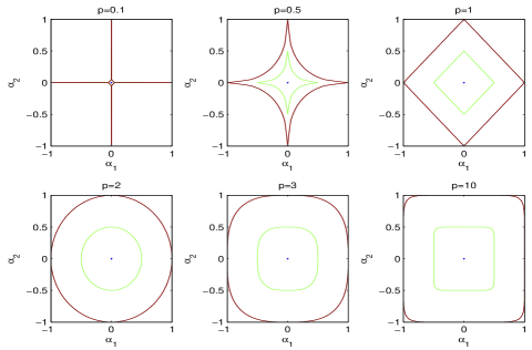
Figure 1: A two-dimensional $p$-space for $p\in\{0.1,0.5,1,2,3,10\}$

3 Proposed Stretchy Regression

3.1 Coefficient Shrinkage

Consider a real integer $q$ defined on the following modified space (called $\tilde{q}$-space for convenience):

$$\|\boldsymbol{\alpha}\|_{\tilde{q}}\mbox{$\triangleq$}\left(\sum^{D}_{i=0}|\alpha_{i}|^{q}\right)^{1/2},$$ (6)

where $q\in\mbox{$\mathbb{R}$}$. When the absolute operator for $\alpha_{i}$ is omitted, we have a modified form for (6) (somewhat related to the generalized mean without averaging) as follows:

$$\|\boldsymbol{\alpha}\|_{q}\mbox{$\triangleq$}\left(\sum^{D}_{i=0}\alpha_{i}^{q}\right)^{1/2}.$$ (7)

In a loose sense, we shall call (7) a $q$-space for convenience hereon (notice that this is not a normed vector space since the scaling property is violated). Fig. 2 shows the $\ell^{p}$-space (5) for $1<p<2$ and the corresponding $\tilde{q}$ (6), $q$ (7) and $q^{2}$-spaces within the same interval. Here we see that the plots for $\tilde{q}$-space show much resemblance to those of $\ell^{p}$-space (5). From the bottom two panels of Fig. 2, we see that the positive quadrant of the solution of real $q$-space and $q^{2}$-space fits well to the solution $p$-space for $1<p<2$. This suggests vertices with positive values being feasible solutions for the proposed constrained solution space. This observation shall be exploited in the following development.

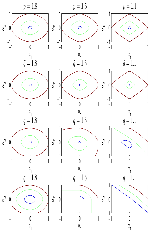
Figure 2: Contour plots at levels 0.1, 0.5 and 1. Top panel: $p$-norms for $p\in\{1.8,1.5,1.1\}$, Second Panel: $\tilde{q}$-space for $q\in\{1.8,1.5,1.1\}$, Third Panel: real $q$-space for $q\in\{1.8,1.5,1.1\}$, Bottom Panel: $q^{2}$-space for $q\in\{1.8,1.5,1.1\}$.

Next, consider the following minimization problem:

$$\min_{\boldsymbol{\alpha}}\|\boldsymbol{\alpha}\|^{2}_{q}+\boldsymbol{\beta}^{T}({\bf y}-{\bf P}\boldsymbol{\alpha}).$$ (8)

Denote the elementwise Hadamard product between vectors $\boldsymbol{a}\in\mbox{$\mathbb{R}$}^{d}$ and $\boldsymbol{b}\in\mbox{$\mathbb{R}$}^{d}$ as $\boldsymbol{a}\circ\boldsymbol{b}$. Also, in order to simplify notations, all the elementwise power terms of vector and matrix in what follows shall be denoted as $\boldsymbol{a}^{q}$ or ${\bf A}^{q}$ except for inverse of square matrix. Let $\bar{\boldsymbol{\alpha}}\mbox{$\triangleq$}[\alpha_{1}^{q/2},\cdots,\alpha_{d}^{q/2}]=\boldsymbol{\alpha}^{q/2}$ where we can write $\|\boldsymbol{\alpha}\|_{q}=(\bar{\boldsymbol{\alpha}}^{T}\bar{\boldsymbol{\alpha}})^{1/2}$. Then take the first derivative of (8) and set it to zero gives:

$$\boldsymbol{\alpha} = \left(\frac{1}{q}{\bf P}^{T}\boldsymbol{\beta}\right)^{\frac{1}{q-1}}.$$ (9)

Based on Newton’s generalized binomial theorem, we consider a scaling vector $\boldsymbol{s}$ which factors out ${\bf P}$ and $\boldsymbol{\beta}$ in the following manner:

$$\left({\bf P}^{T}\boldsymbol{\beta}\right)^{\frac{1}{q-1}} = ({\bf P}^{T})^{\frac{1}{q-1}}\boldsymbol{\beta}^{\frac{1}{q-1}}\circ\boldsymbol{s}.$$ (10)

Then multiply both sides of (9) by ${\bf P}$ and replace ${\bf P}\boldsymbol{\alpha}$ by ${\bf y}$ gives

$$\boldsymbol{\beta} = q\left[\left({\bf P}({\bf P}^{T})^{\frac{1}{q-1}}\right)^{-1}{\bf y}\circ\boldsymbol{s}^{-1}\right]^{q-1}.$$ (11)

Here we note that only the term $\left({\bf P}({\bf P}^{T})^{\frac{1}{q-1}}\right)^{-1}$ involves a full matrix inverse while all other power terms are elementwise operation. Substitute $\boldsymbol{\beta}$ into (9) and simplify gives:

$$\boldsymbol{\alpha} = \left({\bf P}^{T}\right)^{\frac{1}{q-1}}\left[{\bf P}({\bf P}^{T})^{\frac{1}{q-1}}\right]^{-1}{\bf y}.$$ (12)

Notice that apart from the power terms, this solution form is analogous to that of dual ridge regression.

Next, we proceed to convert the above solution in dual space form to its primal form. Based on the matrix identity $({\bf I}+{\bf A}{\bf B})^{-1}{\bf A}={\bf A}({\bf I}+{\bf B}{\bf A})^{-1}$, the solution (12) under dual space can thus be re-written in primal space as

$$\boldsymbol{\alpha}=\left[({\bf P}^{T})^{\frac{1}{q-1}}{\bf P}\right]^{-1}\left({\bf P}^{T}\right)^{\frac{1}{q-1}}{\bf y}.$$ (13)

For data that results in near singularity of the stretched covariances $({\bf P}^{T})^{\frac{1}{q-1}}{\bf P}$ or ${\bf P}({\bf P}^{T})^{\frac{1}{q-1}}$, a regularization term can be included within the inverse term.

In the following experiments, we shall adopt (12) when dealing with under-determined systems and adopt (13) when dealing with over-determined systems.

3.2 First Quadrant Transformation

Consider a stacked set of raw training input data given by

$${\bf X}_{raw}=\stackrel{{\scriptstyle\left[\begin{array}[]{cccc}{\bf x}_{1}&{\bf x}_{2}&\cdots&{\bf x}_{d}\\ \end{array}\right]}}{{\overbrace{\left[\begin{array}[]{cccc}x_{11}&x_{12}&\cdots&x_{1d}\\ x_{21}&x_{22}&\cdots&x_{2d}\\ \vdots&\vdots&\ddots&\vdots\\ x_{M1}&x_{M2}&\cdots&x_{Md}\\ \end{array}\right]}}}=\left[\begin{array}[]{c}\boldsymbol{x}_{1}\\ \boldsymbol{x}_{2}\\ \vdots\\ \boldsymbol{x}_{M}\\ \end{array}\right].$$ (14)

A standardization is first performed for each data column by a $z$-score normalization based on the statistics of training set (mean $\mu_{{\bf x}_{k}}$ and variance $\sigma_{{\bf x}_{k}}$):

$$\underline{{\bf x}}_{k}=({\bf x}_{k}-\mu_{{\bf x}_{k}})/\sigma_{{\bf x}_{k}},\ k=1,...,d.$$ (15)

Then, an exponential function is adopted to map the standardized data into the first quadrant:

$$\breve{{\bf x}}=\exp(a\underline{{\bf x}}_{k}+\boldsymbol{b}_{k}).$$ (16)

Here, we note that the exponential transformation serves two purposes: first quadrant transformation and data warping. The main reason for first quadrant transformation is to handle the power term ($q$) smaller than 2 where complex number arises in the proposed stretchy regression. We call this a key absolute space transformation. The data warping mechanism twists the original data such that large values are differentiated far more than small values or vice versa. This twisting further stretches (or compresses) the relative difference among the input variables on top of the stretchy regression.

4 Synthetic Data

Consider an example with three synthetic data samples as shown in Fig. 3 where the red circle indicates a sample drawn from class-1 distribution ($y=-1$) and the two blue boxes are samples drawn from class-2 distribution ($y=+1$). Since these data are already in first quadrant, no standardization and transformation is necessary. The four sub-figures show the corresponding decision boundaries obtained for a 3rd-order polynomial model at four $q$ values using (12). These results show convergence of learning solutions even though the system is under-determined.

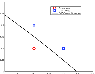
(a) $q=2$	(b) $q=1.5$
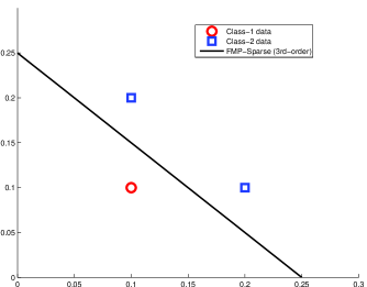
(c) $q=1.3$	(d) $q=1.1$

Figure 3: (a) Decision boundaries (zero threshold value) of a 3rd-order FMP-Sparse model learned from 3 non-overlapping data points at different $q$ values

Table 1 and Fig. 4 show the variation of learned polynomial coefficients ($\boldsymbol{\alpha}=[\alpha_{0},...,\alpha_{9}]$) for the 3rd-order system corresponding to different $q$ values. These results show convergence to sparse solution when $q\rightarrow 1$.

Table 1: Estimated coefficient values over variation of $q$ values for a 3rd-order full polynomial based on 3 data samples

	$q=5$	$q=2$	$q=1.75$	$q=1.5$	$q=1.3$	$q=1.1$
$\alpha_{0}$	-3.934	-4.726	-4.852	-4.956	-4.996	-5.000
$\alpha_{1}$	12.013	17.881	18.856	19.662	19.967	20.000
$\alpha_{2}$	12.013	17.881	18.856	19.662	19.967	20.000
$\alpha_{3}$	14.754	3.624	1.761	0.394	0.019	0.000
$\alpha_{4}$	16.268	5.459	3.107	0.985	0.103	0.000
$\alpha_{5}$	16.268	5.459	3.107	0.985	0.103	0.000
$\alpha_{6}$	13.646	0.729	0.185	0.012	0.000	0.000
$\alpha_{7}$	13.646	0.729	0.185	0.012	0.000	0.000
$\alpha_{8}$	15.510	1.280	0.405	0.041	0.001	0.000
$\alpha_{9}$	15.510	1.280	0.405	0.041	0.001	0.000

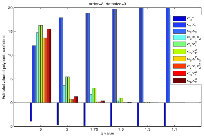
Figure 4: Estimated coefficient values versus $q$ value ($q\in\{2,1.75,1.5,1.3,1.1\}$) based on the 3-samples data

5 Experiments on Prostate Cancer Data

5.1 Linear model fitting

The data for this experiment was adopted in [11] which came from a study in [12]. The correlation between the level of prostate-specific antigen and several clinical measures were studied in men who were to receive a radical prostatectomy. There are eight input variables with one response output. Among the total 97 samples, 67 samples are used for training and the remaining 30 samples are used for testing.

The 8 input variables are standardized by a Matlab zscore normalization (15) and then transformed by (16) with empirically chosen $a=1$ and $\boldsymbol{b}=\boldsymbol{\mu}$ for each dimension to move the data to the first quadrant. Following the example in [11], a linear model is adopted in this experiment. In other words, including the intercept term, we have 9 parameters to be estimated.

The estimated weight parameters for the proposed stretchy regression for each input variable including an intercept are shown in Fig. 5 and Table 2 for $q\in\{5,2,1.4,1.3,1.2,0,-0.5,-5\}$. Here we see stretching beyond the positive and negative $q$ values can be feasible with reasonable accuracy. These results show comparable test accuracy with that of lasso [7] and elastic-net [10]. In terms of model parameters, the results of lasso-elastic-net from the statistical package of [13] as shown in Fig. 6 and Table 3 show better convergence to sparsity.

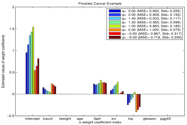
Figure 5: Stretchy regression: estimated coefficient values versus $q$ values ($q\in\{5,2,1.4,1.3,1.2,0,-0.5,-5\}$) for the prostate cancer data.

Table 2: Stretchy regression: estimated coefficient values over variation of $q$ values for prostate cancer data

parameter $\setminus$ $q$	$5$	$2$	$1.4$	$1.3$	$1.2$	$0$	$-0.5$	$-5$
$\alpha_{0}$: intercept	0.954	1.137	1.347	1.425	1.539	0.547	0.645	0.817
$\alpha_{1}$: lcavol	0.153	0.119	0.082	0.065	0.034	0.240	0.214	0.179
$\alpha_{2}$: lweight	0.002	0.002	0.001	0.001	0.000	-0.000	0.001	0.002
$\alpha_{3}$: age	-0.000	-0.000	-0.000	-0.000	-0.000	0.000	0.000	-0.000
$\alpha_{4}$: lbph	0.236	0.213	0.226	0.253	0.320	0.263	0.268	0.255
$\alpha_{5}$: svi	0.085	0.119	0.184	0.218	0.277	0.008	0.034	0.065
$\alpha_{6}$: lcp	-0.246	-0.191	-0.125	-0.074	0.042	-0.408	-0.360	-0.294
$\alpha_{7}$: gleason	-0.000	-0.000	0.000	0.000	0.000	-0.000	-0.000	-0.000
$\alpha_{8}$: pgg45	0.000	0.000	-0.000	-0.000	-0.000	0.000	0.000	0.000
MSE	0.652	0.609	0.533	0.565	0.883	1.022	0.867	0.718
STD	0.225	0.193	0.117	0.099	0.185	0.373	0.317	0.256

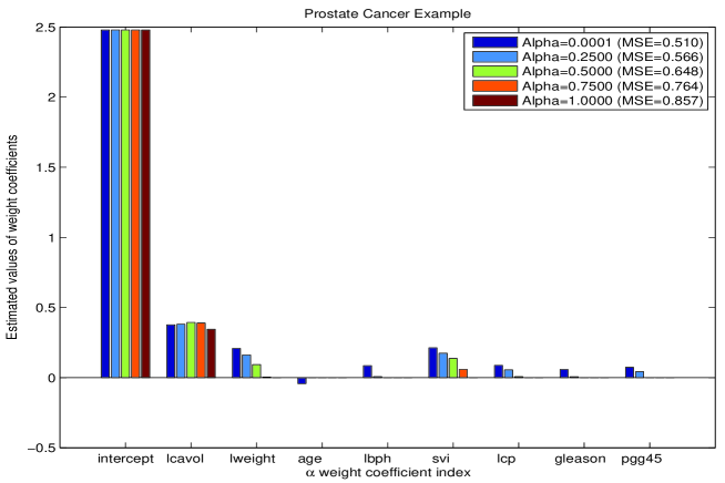
Figure 6: Lasso: estimated coefficient values versus Alpha values (Alpha$\in\{0.0001,0.25,0.5,0.75,1\}$) at Lambda=0.5 for the prostate cancer data.

Table 3: Lasso: estimated coefficient values over variation of Alpha values at Lambda=0.5 for prostate cancer data

parameter $\setminus$ Alpha	$0.0001$	$0.25$	$0.50$	$0.75$	$1.00$
$\alpha_{0}$: intercept	2.478	2.478	2.478	2.478	2.478
$\alpha_{1}$: lcavol	0.377	0.381	0.393	0.389	0.345
$\alpha_{2}$: lweight	0.208	0.162	0.093	0.004	0.000
$\alpha_{3}$: age	-0.042	0.000	0.000	0.000	0.000
$\alpha_{4}$: lbph	0.086	0.008	0.000	0.000	0.000
$\alpha_{5}$: svi	0.213	0.174	0.137	0.059	0.000
$\alpha_{6}$: lcp	0.087	0.056	0.007	0.000	0.000
$\alpha_{7}$: gleason	0.058	0.007	0.000	0.000	0.000
$\alpha_{8}$: pgg45	0.073	0.043	0.000	0.000	0.000
MSE	0.510	0.566	0.648	0.764	0.857

5.2 Full polynomial model fitting

In this experiment, we test the proposed stretchy regression with high order polynomial models. Due to the large number of high order polynomial product terms available for fitting, the inputs need appropriate scaling. We empirically found that $a=10^{-5}$ and $\boldsymbol{b}=a\boldsymbol{\mu}$ for each dimension in (16) and $q=1.0001$ provides reasonable performance. The small $a$ value is to scale the large summation of polynomial product terms while a $q$ value relatively ‘close’ to 1 can stretch the suppression of parameters. To improve the stability of taking inverse of such a large matrix, a regularization term of $10^{-4}$ is included in the matrix inverse term during estimation. A stretchy dual ridge regression is performed since the system is over-complete.

Table 4 shows the MSE results tabulated over polynomial order settings. The corresponding number of polynomial expansion terms are also tabulated along with the polynomial orders. These results show feasibility of using a high order polynomials on high dimensional data when the computational facility is suffice. Fig. 7 shows the estimated 43758 parameters of the 10th order polynomial model. This example shows the feasibility of high polynomial order adoption. However, an in-depth study is yet desired for practical use since the estimated parameters are of high magnitudes.

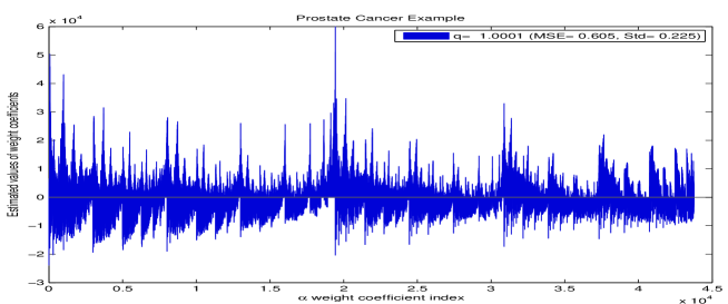
Figure 7: 10th-order full polynomials: estimated coefficient values versus parameter index for the prostate cancer data.

Table 4: Estimation MSE with respect to polynomial order $r$ and number of expansion terms $D$

$r$	1	2	3	4	5	6	7	8	9	10
$D$	9	45	165	495	1287	3003	6435	12870	24310	43758
MSE	0.738	0.497	0.518	0.537	0.549	0.560	0.571	0.584	0.596	0.605

6 Conclusion

A stretchy regression adopting a full multivariate polynomial model was proposed in this article. Essentially, a warped closed-form solution was derived in primal and dual forms analogous to that of ridge regression. Since the solution operated upon positive real input values, an exponential transformation was proposed to convert the inputs to the first quadrant of real axes. Our preliminary experiments show effectiveness of the proposed method in terms of compressive regression.

References

- [1] W. R. Wade, An Introduction to Analysis, 2nd ed. Upper Saddle River, NJ: Prentice Hall, 2000.
- [2] K.-A. Toh, Q.-L. Tran, and D. Srinivasan, “Benchmarking a reduced multivariate polynomial pattern classifier,” IEEE Trans. Pattern Analysis and Machine Intelligence, vol. 26, no. 6, pp. 740–755, 2004.
- [3] R. O. Duda, P. E. Hart, and D. G. Stork, Pattern Classification, 2nd ed. New York: John Wiley & Sons, Inc, 2001.
- [4] K.-A. Toh, “Deterministic neural classification,” Neural Computation, vol. 20, no. 6, pp. 1565–1595, June 2008.
- [5] A. E. Hoerl and R. W. Kennard, “Ridge regression: Biased estimation for nonorthogonal problems,” Technometrics, vol. 12, pp. 55–67, 1970.
- [6] ——, “Ridge regression: Applications to nonorthogonal problems,” Technometrics, vol. 12, pp. 69–82, 1970.
- [7] R. Tibshirani, “Regression shrinkage and selection via the lasso,” J. Roy. Statist. Soc. Ser. B, vol. 58, pp. 267–288, 1996.
- [8] A. Miller, Subset Selection in Regression. London: CHAPMAN & HALL/CRC (A CRC Press Company), 2002.
- [9] I. E. Frank and J. H. Friedman, “A statistical view of some chemometrics regression tools,” Technometrics, vol. 35, pp. 109–148, 1993.
- [10] H. Zou and T. Hastie, “Regularization and variable selection via the elastic net,” Journal of the Royal Statistical Society, Series B, vol. 67, pp. 301–320, 2005, (Part 2).
- [11] T. Hastie, R. Tibshirani, and J. Friedman, The Elements of Statistical Learning: Data Mining, Inference, and Prediction. New York: Springer, 2001.
- [12] T. Stamey, J. Kabalin, J. McNeal, I. Johnstone, F. Freiha, E. Redwine, and N. Yang, “Prostate specific antigen in the diagnosis and treatment of adenocarcinoma of the prostate II. radical prostatectomy treated patients,” Journal of Urology, vol. 16, pp. 1076–1083, 1989.
- [13] The MathWorks, “Matlab and simulink,” in [http://www.mathworks.com/], 2014.