Fooled by bursts. A Goal per Minute model for the World Cup.

Abstract

On the occasion of the last FIFA World Cup in Brazil, The Economist published a plot depicting how many goals have been scored in all World Cup competitions until present, minute by minute. The plot was followed by a naive and poorly grounded qualitative analysis. In the present article we use The Economist dataset to check its conclusions, update previous results from literature and offer a new model. In particular, it will be shown that first and second half game have different scoring rates. In the first half the scoring rate can be considered constant. In the second it increases linearly with time.

Keywords. Goal, distribution, football, soccer, FIFA World Cup, outlier, The Economist

1 Introduction

The Economist [3] is a well known weekly newspaper of economics and economics related subjects. Frequently, it publishes interesting quantitative information in paper and on the web, especially in the Daily chart section. In occasion of the 2014 World Cup it collected the amount of goals scored during all the World Cup competitions, from 1930 to 2014, minute by minute. All the data is presented as interactive plot on the web [6].

We give in Fig.1 a reduction of The Economist original graphic. In our plot additional time (called allowance for time lost in FIFA documentation [5] ) and extra time are not represented. No distinction is made between goals, penalties and own goals. In the original graphic it possible to see in which match each goal was scored and is possible to filter matches according to some categories. The reader interested in these facets should definitely refer to the web. All the data used for this paper and the analysis performed in R [10] software are available at mingotti.uc3m.es/floor1/paper-goals.

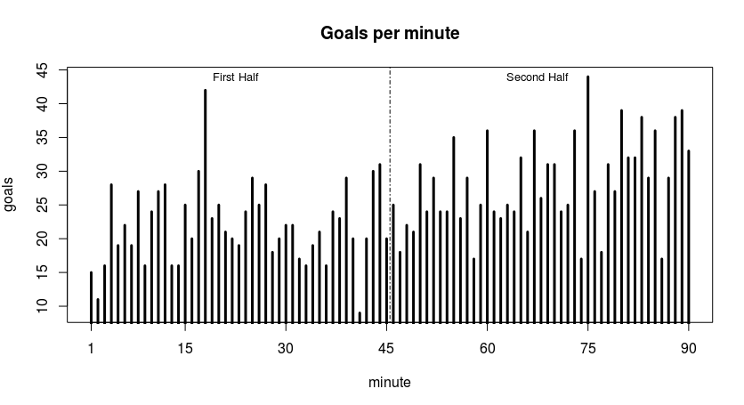
Figure 1: Goals per minute. Reduction of The Economist original plot [6] displaying all goals scored in all World Cup matches until July 2014, minute by minute. Extra time and additional time have been removed.

Just under the original plot the authors summarize the graphical information with the following sentence: “… One can expect a rush of goals in the last ten minutes of normal time, but the 18th and 75th minutes have proved fertile”. We consider such conclusions hurried and possibly lacking in significance. In this paper we will propose a simple and reasonable model that describes the minute by minute goal scoring frequency. After that, we reconsider how much of the original analysis can be confidently accepted.

The goal scoring frequency has been already analyzed in literature for the National Scottish League 1991-1992 in [11], the Australian Soccer League in [1] and the European Champions League in [9]. The 1986 World Cup in [7], 1990 World Cup in [8] and jointly 1998, 2002 and 2006 World Cups in [2]. As far as we could establish, a comprehensive study about goal scoring frequency in all World Cups till present has never been approached.

Article [2] is the most similar to our work. It focuses on World Cup scoring frequency and it considers more than a single tournament. The authors concluded that dividing the match in two 45-min parts, most goals were scored in the second half. Dividing the match in 15-min parts, most of the goals were scored in the last period (76-90) and there was a trend towards more goals scored as time progressed. In this paper we will see all these conclusion can be confirmed and refined using the richer dataset of all World Cups scores.

2 Analysis

From the The Economist original data set we consider only goals scored in regular time, that is in minutes between $[1,45]$ and $[46,90]$. We ignore additional time because its occurrence is decided match per match by the referee [5] and extra time because it depends on the scoring situation at the end of regular time. Their goal scoring rate can not be directly compared with regular time.

Figure 2: Smoothed goals per minute. Goals per minute with a loess smoother (thick line). Numbers near each circle represent minutes. For example, in the first half, the highest number of goals was scored on minute 18th, the least on minute 41th. Dashed line represent half match goal averages. The numerical value of each average is just under each dashed line, on its leftmost side.

We redraw the dataset in Fig.1 with a loess smoother. In Fig.2 the thick continuous line is the smooth loess non parametric fit for the relation between goals and minute. The dashed lines represent the average number of goals in the first and second half respectively. Just under the dashed lines, on their left side, do lay the numerical values of each mean. The parameters used for the loess are the ones default with R [12, 4, 10]

From Fig.2 we can see the average number of goals in the second half (28.16) is larger than in the first half (22.04). The difference between these averages $D:=\bar{x}_{2}-\bar{x}_{1}$ is statistically greater than zero. In this work significance level is always $\alpha=0.05$. Bootstrapping 10000 times we get $D$ is normally distributed as $N(\mu=6.10,\sigma=1.32)$.

Observing the loess smooth fit in Fig.2 we set the following hypothesis up. In the first half of the game the scoring rate is constant, in the second it grows linearly with time. We also notice that the first minutes could have an inferior scoring rate respect to the other minutes in the first half. That is reasonable, the game starts always in the middle of the field, far from a comfortable scoring position.

On the first half, our probabilistic model is that goals are distributed according to a $\mbox{Multinomial}(n,(p_{1},\dots,p_{45}))$ where $p_{i}=p_{j}$ for all $i,j$ in $1\dots 45$. Performing a $\chi^{2}$ goodness of fit test we get $pval=0.0061$, homogeneity would be rejected. But, if we remove just minute 18th, we get $pval=0.1296$ and homogeneity would be far from rejected. We don’t want to be too much lighthearted in dropping observations to satisfy our model so we reshape the dataset and repeat the test. Instead of considering a match as composed of a sequence of single minutes, we consider it as a sequence of 2, 3 and 5 minutes blocks. For each minutes block we set the associate number of goals as the average number goals scored in each minute making the block. Performing again the $\chi^{2}$ goodness of fit test on the first half, now seen as sequence of 2,3,5 minutes blocks, we get pvalue respectively $(0.23,0.49,0.94)$. With a minimal smoothing reshape we see homogeneity test in far from rejected, without dropping any observation. In conclusion, we are confident that the first half can be considered homogeneous and minute 18th an outlier.

In the second half our working hypothesis is a linear relation between minutes elapsed and goals scored. We begin fitting a simple linear regression model with minute as independent variable. By the t-test, minute is a significant variable, $pval=0.00368$. Residuals can be considered normally distributed according to Kolmogorov-Smirnov and Shaipiro-Wilk normality test, which give respectively pvalues $(0.73,0.60)$. $R^{2}=0.18$ is little and not much interesting for us. The fitted model appears in Eq.1

$$goals=13.346+0.0708*minute$$ (1)

From Eq.1 we can get the expected number of goals in minute $m\in(46,\dots,90)$. We will call these values $\hat{\mathbf{g}}_{2nd}:=(\hat{g}_{46},\dots,\hat{g}_{90})$. Normalizing $\hat{\mathbf{g}}$ we get ${\hat{\mathbf{p}}}_{2nd}:=\hat{\mathbf{g}}_{2nd}*(\sum_{i=46}^{90}{\hat{g_{i}}})^{-1}$. And now we can apply again the $\chi^{2}$ to see if the model for the second half is appropriate. Our null hypothesis is that goals realized in the second half ($\mathbf{g}_{2nd}$) are multinomially distributed with probability vector $\hat{\mathbf{p}}_{2nd}$. The $\chi^{2}$ test returns a pvalue of $0.09$ so the null hypothesis can not be rejected in the second half game.

Let us join the half time models and check hypotheses against the full length match data. According to our models, the expected goal sequence is $(\tilde{g}_{1},\dots,\tilde{g}_{90})$. Where $\tilde{g}_{i}$ for $i\in[1,45]$ is the average number of goals scored in the first half and $\tilde{g}_{i}$ for $i\in[46,90]$ is set by Eq.1. Normalizing $\mathbf{\tilde{g}}$ we get a probabilities vector $\mathbf{\tilde{p}}$, a graphical representation of it appears in Fig.3. Using again a $\chi^{2}$, we test if goals scored in all Word Cups matches minute per minute can be a realization of a multinomial distribution with probabilities vector $\mathbf{\tilde{p}}$. We get a $pvalue=0.0034$. Removing observation 18th we get $pval=0.0524$ and we can not reject. Removing also the first three minutes improves the fit giving $pval=0.1245$. To avoid removing observation we reshape the dataset in blocks of 2,3,5 minutes as done previously. The resulting pvalues are respectively $(0.86,0.95,0.99)$ so, the null hypothesis is never rejected. Fig.4 illustrates goals smoothing on reshaping minute variable.

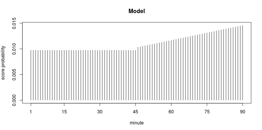
Figure 3: The simple scoring model. If there is a goal in a match of the World Cup it will happen at some minute with the probability here depicted. In the first half game the probability is constant, in the second it grows linearly with time.

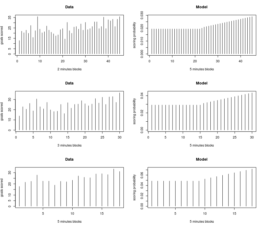
Figure 4: This figure represents how reshaping variable minute in blocks of 2,3,5 units affects the goals distribution.

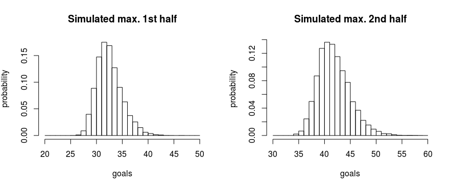
Figure 5: Simulated maxima distribution for the first and second half. These two histograms tell us that 42 goals, as a maximum in the first half, is an unexpected result. On the contrary, 44 goals as a maximum for on the second half is not surprising.

An analytic description of the probability distribution can be easily obtained once we move to a time continuous description. Rescaling the match to a $[0,1]$ duration interval, if there will be a goal, the probability it will happen before time $x$ will be given by $F(x)$. $F$ is defined in Eq.2.

$$F(x)=\begin{cases}0.878264\ x,&\quad 0\leq x<0.5\\ 0.381889\ x^{2}+0.548938\ x+0.069173,&\quad 0.5\leq x<1\\ 1&\quad x\geq 1\\ \end{cases}$$ (2)

Minutes 18th and 75th were called in the original document “fertile” minutes. Using our model we have a different interpretation for each one of them. In Fig.5 we see the simulated distribution of the maximum in the first and second half according to the model. For the first half we see that an observation larger than the 18th (42 goals) is improbable, its probability is approximately 0.0015. On the contrary, one observation larger than the 75th (44 goals) in the second half it is not improbable at all ($p\approx 0.217$).

3 Conclusions

There is enough evidence to state that the goal scoring distribution in the World Cup matches can be considered constant in the first half game and growing linearly in the second half. Dividing the game in blocks of 2, 3 or 5 minutes confirms the model is valid and makes is more robust to extreme values. An analytic cumulative distribution function for goal scoring is presented in Eq.2.

Previous finding in article [2] are confirmed, there are more goals in the second half respect to the first one. According to our model, if there is a goal in a match, the probability that it will be in the first half is $44\%$. The last part of the game is most probable for a goal, and there is a trend toward more goals as time passes, but only in the second half.

The Economist conclusions about its dataset are only partially acceptable. Indeed, it is true that in on the last part of the game there are expected more goals. It is not true that minute 75th is an especially “fertile” minute, a maximum of 44 goals can be easily realized by the variability of the second half game. Minute 18th is more interesting, according to our model the probability of observing a maximum of 42 goals in the first half is about $2\cdot 10^{-3}$. We guess it has to be considered an outlier and removed because it is an isolated burst, it has no connections with its neighboring values. Performing a mild smooth, as grouping each match as a sequence of 2 minutes removes all of its importance.

References

- [1] GA Abt, G Dickson, and WK Mummery. Goal scoring patterns over the course of a match: an analysis of the Australian national soccer league. Science and football IV, page 106, 2002.
- [2] V Armatas, A Yiannakos, and P Sileloglou. Relationship between time and goal scoring in soccer games: Analysis of three world cups. International Journal of Performance Analysis in Sport, 7(2):48–58, 2007.
- [3] The Economist. http://www.economist.com, 2014.
- [4] Julian J Faraway. Extending the linear model with R: generalized linear, mixed effects and nonparametric regression models. CRC press, 2005.
- [5] FIFA: Law 7. Duration of the match. http://goo.gl/tcd5B2, 2014.
- [6] Goooooaaaaaaaallllll! http://www.economist.com/node/21603828, 2014.
- [7] X Jinshan. The analysis of the techniques, tactics and scoring situations of the 13th world cup. Sandong Sports Science and Technique (April), pages 89–91, 1986.
- [8] X Jinshan, C Xiaoke, K Yamanaka, and M Matsumoto. Analysis of the goals in the 14th world cup. Science and football II, pages 203–205, 1993.
- [9] C Michailidis, I Michailidis, G Papaiakovou, and I Papaiakovou. Analysis and evaluation of way and place that goals were achieved during the european champions league of football 2002-2003. Sports Organization, 2(1):48–54, 2004.
- [10] R: A language and environment for statistical computing, 2012. ISBN 3-900051-07-0.
- [11] T Reilly. Motion analysis and physiological demand. Science and football III, pages 65–81, 1997.
- [12] William N Venables and Brian D Ripley. Modern applied statistics with S. Springer, 2002.