Topological BF theory of the quantum hydrodynamics of incompressible polar fluids

Abstract

We analyze a hydrodynamical model of a polar fluid in (3+1)-dimensional spacetime. We explore a spacetime symmetry – volume preserving diffeomorphisms – to construct an effective description of this fluid in terms of a topological BF theory. The two degrees of freedom of the BF theory are associated to the mass (charge) flows of the fluid and its polarization vorticities. We discuss the quantization of this hydrodynamic theory, which generically allows for fractionalized excitations. We propose an extension of the Girvin-MacDonald-Platzman algebra to (3+1)-dimensional spacetime by the inclusion of the vortex-density operator in addition to the usual charge density operator and show that the same algebra is obeyed by massive Dirac fermions that represent the bulk of $\mathbb{Z}^{\,}_{2}$ topological insulators in three-dimensional space.

I Introduction

One of the most prominent topological phenomena in quantum matter is the quantum Hall effect.QHE-Book It comes about when a two dimensional electron gas is subject to a strong perpendicular magnetic field at sufficiently low temperatures. The striking property of this many-body state, its quantized transport, derives from an incompressible (i.e., gapped) state in the bulk accompanied by soft chiral edge modes along the one dimensional boundary. The electrons from the bulk state can be thought of as giving rise to an incompressible fluid state.

The incompressible fluid picture of the quantum Hall effect has been investigated by Bahcall and Susskind, Bahcall91 ; Susskind01 who have shown that some properties of the quantum Hall state can be accounted for if one considers a classical two dimensional incompressible fluid model of charged point particles in a perpendicular magnetic field and if one applies a semi-classical analysis thereof.

In the construction presented in Refs. Bahcall91, and Susskind01, , the fluid description arises by considering the limit when the inter-particle distance is sufficiently small. In this limit, the individual positions of particles can be effectively described by a collective coordinate of the fluid. The freedom to relabel the discrete particles emerges as a gauge symmetry in the fluid formulation (see, for instance, the review in Ref. Jackiw04, ). The classical Lagrangian of the fluid of charged particles contains an (Abelian) Chern-Simons term whose vector field undergoes a gauge transformation that is equivalent to a reparametrization of the fluid’s underlying particles. Given that the Chern-Simons action captures the topological essence of the quantum Hall state, the fluid formulation of the Hall effect discussed in Refs. Bahcall91, and Susskind01, offers an insightful platform for understanding the interplay of incompressibility and topology as it relates to two dimensional systems in an applied magnetic field.

In recent years, a number of new topological phenomena has arisen that go beyond the quantum Hall paradigm. In particular, topological band insulators in two and three dimensions have been predicted and experimentally found in solid state systems. Hasan2010 ; Qi2011 The discovery of this new class of materials has revitalized the interest for non-interacting Schnyder2008 ; Kitaev2009 ; Ryu2010 and interacting Levin2009 ; Neupert2011 ; Santos2011 ; Chen2012 ; Lu2012 ; Vishwanath2013 ; Wang2014 topological phases of matter.

Motivated by the construction of Refs. Bahcall91, and Susskind01, , we propose a fluid model in three dimensional space whose effective action contains a BF topological term, Blau1991 the natural generalization of the Chern-Simons term to three dimensions. The new feature of our model, aside from the dimensionality three of space, is that, in order to obtain a topological BF term, we are led to consider a polar incompressible fluid, while the fluid is made of point particles in Refs. Bahcall91, and Susskind01, . We propose a Lagrangian written in the explicit coordinates of the fluid’s particles, position and dipole field, and show that, by expressing this term as a function of the small fluctuations of the particle’s positions, it renders a topological BF action.

The BF term captures the Berry phase associated to a point defect adiabatically winding around a vortex line. Blau1991 ; Bergeron1995 ; Szabo1998 ; Hansson2004 ; Cho2011 The Berry phase associated to this adiabatic motion yields the statistics between point and vortex defects in three dimensions. In our formulation, the coefficient of the BF action emerges as a function of the phenomenological parameters of the fluid, which is subsequently shown to satisfy a quantization condition upon quantization of the fluid.

We also find that the BF theory furnishes a pair of conserved currents, i.e., a charge current and a vorticity current. We interpret these currents within a massive Dirac model as the usual fermion current and the fermion “vorticity” current respectively. Upon evaluation the algebra for the projected charge and spin densities in the Dirac model, we find that it agrees with the BF algebra. We find an algebra very similar to the celebrated Girvin-MacDonald-Platzman (GMP) algebra for FQH systems, with the inclusion of a vorticity sector in addition to the charge sector.

This paper is organized as follows. In Sec. II, we provide a short review of Lagrangian fluids focusing on the main aspect related to our work, namely the role played by the invariance under volume preserving diffeomorphisms. In Sec. III, we propose a classical model for a polar incompressible fluid, which leads to BF term effective action once small fluctuations of the fluid are take into account. Quantization of this fluid leads to a the identification of the quasi-particles (point-like and vortex-like) as well as their mutual statistics determined by the BF term. In Sec. IV, we propose an extension of the Girvin-MacDonald-Platzman algebra to (3+1)-dimensional spacetime by the inclusion of the vortex-density operator in addition to the usual charge-density operator and show that the same algebra is obeyed by massive Dirac fermions that represent the bulk of $\mathbb{Z}^{\,}_{2}$ topological insulators in three-dimensional space. Finally, we close with discussions in Sec. V.

II Review of Lagrangian fluids

We begin by reviewing the Lagrangian description of fluids. Jackiw04 We consider a system of identical classical particles, described by coordinates ${\bm{x}}^{\,}_{\beta}(t)$ and velocity fields $\dot{{\bm{x}}}^{\,}_{\beta}(t)$, where $\{\beta\}$ is a discrete set of particle labels. The Lagrangian of the system reads

$$L\equiv\sum_{\beta}\mathcal{L}\Big{(}{\bm{x}}^{\,}_{\beta}(t),\dot{{\bm{x}}}^{\,}_{\beta}(t)\Big{)}.$$ (1)

For identical particles, the choice of the particle label $\beta$ is arbitrary. Correspondingly, the Lagrangian $L$ is invariant under any relabeling of the discrete indices

$$\{\beta\}\to\{\beta^{\prime}\}.$$ (2)

In the hydrodynamical description of the system, one replaces the discrete label $\beta\in\{\beta\}$ by the label ${\bm{y}}\in\mathbb{R}^{3}$, i.e., the coordinate and velocity vectors become vector fields according to the rule

$${\bm{x}}^{\,}_{\beta}(t)\to{\bm{x}}(t,{\bm{y}}),\qquad\dot{{\bm{x}}}^{\,}_{\beta}(t)\to\dot{{\bm{x}}}(t,{\bm{y}}),$$ (3)

respectively. Here, ${\bm{y}}$ can be thought of as a comoving coordinate that labels the position of an infinitesimal droplet of the fluid. Initially, i.e., at $t=0$, we declare that ${\bm{x}}(t=0,{\bm{y}})={\bm{y}}$. In this hydrodynamical limit, the Lagrangian (1) becomes

$$L=\int\,\mathrm{d}^{3}{\bm{y}}\,\rho^{\,}_{0}\,\mathcal{L}\Big{(}{\bm{x}}(t,{\bm{y}}),\dot{{\bm{x}}}(t,{\bm{y}})\Big{)},$$ (4)

where the positive number $\rho^{\,}_{0}$ is interpreted as the mean particle density in ${\bm{y}}$-space.

The invariance of the Lagrangian (1) under any particle relabeling (2) translates, in the fluid description, to an emergent continuous (gauge) symmetry of the Lagrangian (4) with respect to a properly defined reparametrization

$${\bm{y}}\to\tilde{{\bm{y}}}({\bm{y}}).$$ (5a)

To identify this continuous symmetry, we require that the coordinates of the fluid remain invariant, i.e.,

$$\tilde{{\bm{x}}}(t,\tilde{{\bm{y}}})={\bm{x}}(t,{\bm{y}}),$$ (5b)

since the physical position of a particle does not depend on the chosen underlying parametrization. The Lagrangian (4) transforms under the reparametrization (5) as

$$\tilde{L}=\int\mathrm{d}^{3}\tilde{{\bm{y}}}\,\Big{|}\frac{\partial{\bm{y}}}{\partial\tilde{{\bm{y}}}}\Big{|}\,\rho^{\,}_{0}\,\mathcal{L}\Big{(}\tilde{{\bm{x}}}(t,\tilde{{\bm{y}}}),\dot{\tilde{{\bm{x}}}}(t,\tilde{{\bm{y}}})\Big{)}.$$ (6)

Invariance of Eq. (6), i.e., $\tilde{L}=L$, is then achieved provided

$$\Big{|}\frac{\partial{\bm{y}}}{\partial\tilde{{\bm{y}}}}\Big{|}=1.$$ (7)

Condition (7) defines a volume preserving diffeomorphism (VPD) if we assume that the map (5a) is sufficiently smooth.

An infinitesimal VPD is defined by

$$\delta^{\,}_{{\bm{f}}}\,y^{\,}_{i}:=\tilde{y}^{\,}_{i}-y^{\,}_{i}=-f^{\,}_{i}(\bm{y}),\qquad i=1,2,3,$$ (8a)

where the infinitesimal vector field $$\bm{f}$$ must be divergence free,

$$\partial^{\,}_{i}\,f^{\,}_{i}=0,$$ (8b)

in order to meet condition (7). Here and throughout,

$$\partial^{\,}_{i}\equiv\frac{\partial}{\partial y^{\,}_{i}},\qquad i=1,2,3.$$ (8c)

In three dimensional space, the divergence-free vector field $\bm{f}$, with the components $f^{\,}_{i}$ defined in Eq. (8) for $i=1,2,3$ carrying the dimension of length, can always be parametrized (in a non-unique way) as

$$f^{\,}_{i}=\epsilon^{\,}_{ijk}\,\partial^{\,}_{j}\zeta^{\,}_{k}$$ (9)

for any smooth vector field $\bm{\zeta}$ with the components $\zeta^{\,}_{m}$ ($m=1,2,3$) carrying the dimension of area. In the following, summation over repeated indices is implied and sum over the Latin indices run over the three spatial components.

In turn, the variation of the coordinate $\bm{x}$ under the transformation parametrized by ${\bm{f}}$ is defined by

$$\delta^{\,}_{{\bm{f}}}\,\bm{x}(t,\bm{y}):=\tilde{\bm{x}}(t,\bm{y})-\bm{x}(t,\bm{y}).$$ (10)

With the help of Eq. (5b) and upon insertion of the infinitesimal transformation (8),

$$\begin{split}\delta^{\,}_{{\bm{f}}}\,x^{\,}_{i}=&\,f^{\,}_{j}\,\partial^{\,}_{j}\,x^{\,}_{i}\\ =&\,\epsilon^{\,}_{jlm}\,\partial^{\,}_{j}\,x^{\,}_{i}\,\partial^{\,}_{l}\,\zeta^{\,}_{m}.\end{split}$$ (11)

From the invariance of the Lagrangian (4) under arbitrary infinitesimal VPD defined by Eqs. (5) and (7), there follows, according to Noether’s theorem, the constant of motion

$$\begin{split}C^{\,}_{{\bm{f}}}:=&\,\int\mathrm{d}^{3}{\bm{y}}\,\rho^{\,}_{0}\,\pi^{\,}_{i}\,\delta^{\,}_{{\bm{f}}}\,x^{\,}_{i}\\ =&\,\int\mathrm{d}^{3}{\bm{y}}\,\rho^{\,}_{0}\,\pi^{\,}_{i}\,\epsilon^{\,}_{jlm}\,\partial^{\,}_{j}\,x^{\,}_{i}\,\partial^{\,}_{l}\,\zeta^{\,}_{m}\\ =&\,\int\mathrm{d}^{3}{\bm{y}}\,\rho^{\,}_{0}\,\Big{(}\epsilon^{\,}_{mlj}\partial^{\,}_{l}\,\pi^{\,}_{i}\,\partial^{\,}_{j}\,x^{\,}_{i}\,\Big{)}\zeta^{\,}_{m},\end{split}$$ (12a)

where

$$\pi^{\,}_{i}:=\frac{\partial\,\mathcal{L}}{\partial\,\dot{x}^{\,}_{i}}$$ (12b)

is the canonical momentum and, in deriving Eq. (12), we have made use of integration by parts and we have neglected surface terms. Invariance of Eq. (12) under the infinitesimal coordinate transformation (11) for an arbitrary vector field $\bm{\zeta}$ yields the local conservation law

$$\frac{\mathrm{d}\bm{\Lambda}}{\mathrm{d}t}=0$$ (13a)

for the vector field $$\bm{\Lambda}$$ with the components

$$\Lambda^{\,}_{i}:=\epsilon^{\,}_{ijk}\,\partial^{\,}_{j}\,\pi^{\,}_{l}\,\partial^{\,}_{k}\,x^{\,}_{l},\quad i=1,2,3.$$ (13b)

The vector field $\bm{\Lambda}$ carries the dimension of energy multiplied by time per area.

The local density of the fluid is defined by

$$\rho(t,\bm{y}):=\rho^{\,}_{0}\,J\,\left(\frac{\partial{\bm{y}}}{\partial{\bm{x}}}\right)(t,\bm{y}),$$ (14a)

where

$$J\left(\frac{\partial{\bm{x}}}{\partial{\bm{y}}}\right):=\left|\epsilon^{\,}_{ijk}\frac{\partial x^{\,}_{1}}{\partial y^{\,}_{i}}\frac{\partial x^{\,}_{2}}{\partial y^{\,}_{j}}\frac{\partial x^{\,}_{3}}{\partial y^{\,}_{k}}\right|=1\Big{/}J\left(\frac{\partial{\bm{y}}}{\partial{\bm{x}}}\right)$$ (14b)

is the Jacobian that relates the infinitesimal volume element $\mathrm{d}^{3}\bm{y}$ to the infinitesimal volume element $\mathrm{d}^{3}\bm{x}(t,\bm{y})$. Starting with ${\bm{x}}(t=0,{\bm{y}})={\bm{y}}$ yields an initially uniform fluid density $\rho(t=0,\bm{y})=\rho^{\,}_{0}$.

We define an antisymmetric two-form with the components

$$b^{\,}_{ij}=-b^{\,}_{ji},\qquad i,j=1,2,3,$$ (15a)

through

$$\epsilon^{\,}_{ijk}\,b^{\,}_{jk}(t,{\bm{y}}):=\rho^{\,}_{0}\left[x^{\,}_{i}(t,{\bm{y}})-y^{\,}_{i}\right],\qquad i=1,2,3.$$ (15b)

The vector field with the components $\epsilon^{\,}_{ijk}\,b^{\,}_{ij}$ carries the dimensions of inverse area and is proportional to the deviation between the coordinate $x^{\,}_{i}(t,{\bm{y}})$ at time $t$ and its initial value $\bm{y}$ at time $t=0$. Assuming small deviations of the fluid density away from $\rho^{\,}_{0}$, we may treat the two-form $b^{\,}_{ij}=-b^{\,}_{ji}$ as small. In terms of this field, the density of the fluid is given by

$$\rho=\rho^{\,}_{0}-\epsilon^{\,}_{ijk}\,\partial^{\,}_{i}b^{\,}_{jk}+\cdots,$$ (16)

where $\cdots$ stands for higher order terms in $b^{\,}_{ij}$. One verifies that the transformation law

$$b^{\,}_{jk}\to b^{\,}_{jk}+\partial^{\,}_{j}\chi^{\,}_{k}-\partial^{\,}_{k}\chi^{\,}_{j}$$ (17)

does not alter the density (16) provided the vector field $\bm{\chi}$ with the components $\chi^{\,}_{i}$ for $i=1,2,3$ is smooth, i.e., $\partial^{\,}_{j}\partial^{\,}_{k}\chi^{\,}_{i}=\partial^{\,}_{k}\partial^{\,}_{j}\chi^{\,}_{i}$. Equation (17) can also be obtained with the identification $\bm{\chi}=\rho^{\,}_{0}\,\bm{\zeta}/2$ from

$$\epsilon^{\,}_{ijk}\left(\tilde{b}^{\,}_{jk}(t,\bm{y})-b^{\,}_{jk}(t,\bm{y})\right):=\rho^{\,}_{0}\left[\tilde{x}^{\,}_{i}(t,\bm{y})-x^{\,}_{i}(t,\bm{y})\right].$$ (18)

Hereto, one makes use of the fact that the 2-tensor field is antisymmetric on the left-hand side, while one makes use of the linearized version of Eq. (11), whereby the approximation $\partial^{\,}_{j}x^{\,}_{i}\approx\delta^{\,}_{ij}$ is done, on the right-hand side. The invariance of the local density (16) under the transformation (17) thus reflects the invariance of the Lagrangian (4) under any VPD defined by Eqs. (5) and (7).

We close this review of Lagrangian fluids with the example defined by the Lagrangian

$$L^{\,}_{\mathrm{free}}:=\int\,\mathrm{d}^{3}{\bm{y}}\,\rho^{\,}_{0}\,\mathcal{L}^{\,}_{\mathrm{free}}$$ (19a)

with the local Lagrangian

$$\mathcal{L}^{\,}_{\mathrm{free}}:=\frac{m}{2}\,\dot{\bm{x}}^{2}.$$ (19b)

This Lagrangian describes a fluid of non-interacting and identical classical particles of mass $m$. The canonical momentum (12) becomes the usual impulsion

$$\bm{\pi}=m\,\dot{\bm{x}}.$$ (20)

The local conserved vector field (13b) becomes

$$\Lambda^{\,}_{i}=m\,\epsilon^{\,}_{ijk}\,\partial^{\,}_{j}\,\dot{x}^{\,}_{l}\,\partial^{\,}_{k}\,x^{\,}_{l},$$ (21)

whose conserved integral is called the vortex helicity and is related to a Chern number (see Ref. Jackiw04, ). In terms of the two-form defined in Eq. (15b), the canonical momentum is (exactly) given by

$$\pi^{\,}_{i}=\frac{m}{\rho^{\,}_{0}}\,\epsilon_{ijk}\,\dot{b}^{\,}_{jk},$$ (22)

while the vortex helicity (21) is given by

$$\Lambda^{\,}_{i}=2\,\frac{m}{\rho^{\,}_{0}}\,\partial^{\,}_{j}\dot{b}^{\,}_{ij}+\cdots$$ (23)

to leading order in powers of the two-form defined in Eq. (15b).

III BF Lagrangian for an incompressible polar fluid

III.1 Definition

We start from the discrete set $\{\beta\}$ that labels identical particles with a mass $m$. We associate to any label $\beta$ the coordinate $\bm{x}^{\,}_{\beta}(t)$, the velocity $\dot{\bm{x}}^{\,}_{\beta}(t)$, and the polar vector $\bm{d}^{\,}_{\beta}(t)$ whose dimension we choose for later convenience to be that of an inverse length. We then endow a Lagrangian dynamics to these degrees of freedom by defining

$$L^{\,}_{\mathrm{pol}}:=\sum_{\beta}\mathcal{L}^{\,}_{\mathrm{pol}}\Big{(}\dot{{\bm{x}}}^{\,}_{\beta}(t),{\bm{d}}^{\,}_{\beta}(t)\Big{)}$$ (24a)

where

$$\mathcal{L}^{\,}_{\mathrm{pol}}\Big{(}\dot{{\bm{x}}}^{\,}_{\beta}(t),{\bm{d}}^{\,}_{\beta}(t)\Big{)}:=-\frac{g}{2\pi}\,{\bm{d}}^{\,}_{\beta}(t)\cdot\dot{{\bm{x}}}^{\,}_{\beta}(t).$$ (24b)

The real-valued coupling $g$ carries the dimension of energy multiplied by time. The multiplicative factor $(-1)/(2\pi)$ is chosen for later convenience.

The hydrodynamic limit of the Lagrangian (24) is the Lagrangian polar fluid

$$L^{\,}_{\mathrm{pol}}:=\int\,\mathrm{d}^{3}{\bm{y}}\,\rho^{\,}_{0}\,\mathcal{L}^{\,}_{\mathrm{pol}},$$ (25a)

with the local Lagrangian

$$\mathcal{L}^{\,}_{\mathrm{pol}}:=-\frac{g}{2\pi}\,{\bm{d}}\cdot\dot{{\bm{x}}}$$ (25b)

carrying the dimension of energy, for the positive number $\rho^{\,}_{0}$ is again interpreted as the mean particle density in ${\bm{y}}$-space.

The Lagrangian density (25b) is invariant under simultaneous rotations of the coordinate and polar vectors. Moreover, it is the unique scalar that is linear in both $\bm{d}$ and ${\bm{x}}$ and of first order in the time derivative, up to a total time derivative. In addition to the rotational symmetry, two discrete symmetries are notable. The first is parity,

$$\mathcal{P}:\quad\begin{cases}{\bm{d}}(t,\bm{y})\to-{\bm{d}}(t,\bm{y}),\\ {\bm{x}}(t,\bm{y})\to-{\bm{x}}(t,\bm{y}),\\ \dot{{\bm{x}}}(t,\bm{y})\to-\dot{{\bm{x}}}(t,\bm{y}).\end{cases}$$ (26)

The second is time-reversal symmetry

$$\mathcal{T}^{\,}_{\pm}:\quad\begin{cases}{\bm{d}}(t,\bm{y})\to\pm{\bm{d}}(-t,\bm{y}),\\ {\bm{x}}(t,\bm{y})\to+{\bm{x}}(-t,\bm{y}),\\ \dot{{\bm{x}}}(t,\bm{y})\to-\dot{{\bm{x}}}(-t,\bm{y}),\end{cases}$$ (27)

where the $\pm$ sign choice depends on the nature of the dipoles. It is $+$ for electric dipoles, while it is $-$ for magnetic dipoles. The Lagrangian density (25b) is invariant under $\mathcal{P}$ and under $\mathcal{T}^{\,}_{-}$ (applicable to magnetic moments). Most importantly, the polar fluid is invariant under any VPD defined by Eqs. (5) and (7). We focus primarily on the invariance under VPD.

We are after the local density

$$\rho(t,{\bm{y}}):=\rho^{\,}_{0}\,J\left(\frac{\partial{\bm{y}}}{\partial{\bm{x}}}\right)$$ (28a)

and the local conserved Noether vorticity field $$\bm{\Lambda}$$ with the components

$$\begin{split}\Lambda^{\,}_{i}:=&\,\epsilon^{\,}_{ijk}\,\partial^{\,}_{j}\,\pi^{\,}_{l}\,\partial^{\,}_{k}\,x^{\,}_{l}\\ =&\,-\frac{g}{2\pi}\,\epsilon^{\,}_{ijk}\frac{\partial d^{\,}_{l}}{\partial y^{\,}_{j}}\frac{\partial x^{\,}_{l}}{\partial y^{\,}_{k}}\end{split}$$ (28b)

for $i=1,2,3$. The density is even under either the transformation (26) or the transformation (27). The vortex helicity is odd under either the transformation (26) or the transformation (27).

We parametrize the coordinates $x^{\,}_{1},x^{\,}_{2},x^{\,}_{3}$ according to

$$x^{\,}_{i}(t,{\bm{y}})=:y^{\,}_{i}+\frac{1}{\rho^{\,}_{0}}\,\epsilon^{\,}_{ijk}\,b^{\,}_{jk}(t,{\bm{y}}).$$ (29)

As was the case with Eq. (15b), the antisymmetric two-form with the components $b^{\,}_{jk}(t,{\bm{y}})=-b^{\,}_{kj}(t,{\bm{y}})$ encodes, up to a contraction with $(1/\rho^{\,}_{0})\,\epsilon^{\,}_{ijk}$, the deviation between the comoving coordinate $\bm{y}$ and the coordinate $\bm{x}^{\,}(t,\bm{y})$ at time $t$ in the polar fluid.

Under the assumptions that both $b^{\,}_{ij}$ and $\bm{d}$ remain small for all times and for all comoving coordinates, one finds the relations

$$\rho(t,{\bm{y}})=\rho^{\,}_{0}-\epsilon^{\,}_{ijk}\,\partial_{i}b^{\,}_{jk}(t,{\bm{y}})+\cdots,$$ (30a)

and

$$\Lambda^{\,}_{i}(t,{\bm{y}})=-\frac{g}{2\pi}\,\epsilon^{\,}_{ijk}\,\partial^{\,}_{j}d^{\,}_{k}(t,{\bm{y}})+\cdots,$$ (30b)

to linear order in the fields $b^{\,}_{ij}$ and $d^{\,}_{i}$, for the local density (28a) and local vortex helicity (28b), respectively.

Equation (30a) is invariant under the transformation

$$b^{\,}_{jk}\to b^{\,}_{jk}+\partial^{\,}_{j}\chi^{\,}_{k}-\partial^{\,}_{k}\chi^{\,}_{j}$$ (31a)

for any smooth vector field $$\bm{\chi}$$. Equation (30b) is invariant under

$$d^{\,}_{k}\to d^{\,}_{k}+\partial^{\,}_{k}\xi,$$ (31b)

for any smooth scalar field $\xi$. The linearized local density (30a) is even under either the transformation (26) or the transformation (27). The linearized local vortex helicity (30b) is odd under either the transformation (26) or the transformation (27).

The local Lagrangian (25), takes the linearized form (up to total derivatives)

$$\mathcal{L}^{\,}_{\mathrm{pol}}=\frac{g}{2\pi\,\rho^{\,}_{0}}\,\epsilon^{\,}_{ijk}\,\dot{d}^{\,}_{i}\,b^{\,}_{jk},$$ (32)

where we recall that $g$, $\rho^{\,}_{0}$, $d^{\,}_{i}$, and $b^{\,}_{jk}$ carry the dimensions of energy multiplied by time, inverse volume, inverse length, and inverse area, respectively.

A VPD defined by Eqs. (5) and (7) leaves the local density (28a) of the polar fluid invariant. This symmetry is realized by the symmetry under the transformation (31a) of the linearized local density (30a) and must hold at the level of the linearized local Lagrangian (32). Indeed it does, as we now verify. The transformation law of $\mathcal{L}^{\,}_{\mathrm{pol}}$ under the infinitesimal VPD (31a) is

$$\mathcal{L}^{\,}_{\mathrm{pol}}\to\mathcal{L}^{\,}_{\mathrm{pol}}+2\times\frac{g}{2\pi\,\rho^{\,}_{0}}\,\dot{{\bm{d}}}\,\cdot\left({\bm{\nabla}}\wedge{\bm{\chi}}\right).$$ (33)

Since the vector field ${\bm{\chi}}$ is arbitrary, to enforce the symmetry under VPD we must demand that

$$\frac{\mathrm{d}}{\mathrm{d}t}\left({\bm{\nabla}}\wedge{\bm{d}}\right)=0.$$ (34)

Now, Eq. (34) follows from

$$\frac{\mathrm{d}{\bm{\Lambda}}}{\mathrm{d}t}=0,$$ (35)

to linear order, as can be observed from Eq. (30b). [As we did to reach Eq. (13), we are ignoring boundary terms when performing partial integrations.]

The linearized local Lagrangian (32) is proportional to the Lagrangian density of the topological BF field theory defined by Eq. (39) in the temporal gauge defined by the conditions

$$d^{\,}_{0}=0,\qquad b^{\,}_{0i}=0,\qquad i=1,2,3.$$ (36)

A BF field theory is an example of a topological field theory. Topological field theories are interpreted in physics as effective descriptions at long distances, low energies, and vanishing temperature of quantum Hamiltonians with spectral gaps separating the ground state manifolds from all excited states. This observation motivates the following definition. The VPD polar fluid is said to be incompressible if it has the constant density

$$\rho=\rho^{\,}_{0}\;.$$ (37)

Without loss of generality, we consider henceforth a magnetic dipolar fluid, in which any non-vanishing value taken by the conserved quantity ${\bm{\Lambda}}$ breaks the symmetry under $\mathcal{T}^{\,}_{-}$ defined in Eq. (27). We say that the VPD polar fluid is time-reversal symmetric if and only if

$${\bm{\Lambda}}=0.$$ (38)

[The same conclusion is reached for an electric polar fluid, in which case it is the symmetry under $\mathcal{P}$ defined in Eq. (26) that implies ${\bm{\Lambda}}=0$.]

Incompressibility of a time-reversal symmetric (magnetic) polar fluid is automatically implemented with the help of the Lorentz covariant extension of $\mathcal{L}^{\,}_{\mathrm{pol}}$ given by (we set the speed of light $c$ to be unity, $c=1$, and $\mu,\nu,\lambda,\sigma=0,1,2,3$)

$$S^{\,}_{\mathrm{BF}}:=\int\mathrm{d}^{4}y\,\mathcal{L}^{\,}_{\mathrm{BF}},\qquad\mathcal{L}^{\,}_{\mathrm{BF}}:=\frac{g}{2\pi}\,\epsilon^{\mu\nu\lambda\sigma}\,b^{\,}_{\mu\nu}\,\partial^{\,}_{\lambda}d^{\,}_{\sigma}.$$ (39)

Indeed, the equations of motion that follow from $\mathcal{L}^{\,}_{\mathrm{BF}}$ are the conservation laws for the matter current

$$j^{\mu}:=\frac{1}{2\pi}\,\epsilon^{\mu\nu\lambda\sigma}\,\partial^{\,}_{\nu}\,b^{\,}_{\lambda\sigma},\qquad\partial^{\,}_{\mu}j^{\mu}=0,$$ (40)

and for the vortex-helicity currents

$$J^{\mu\nu}:=\frac{1}{2\pi}\,\epsilon^{\mu\nu\lambda\sigma}\,\partial^{\,}_{\lambda}d^{\,}_{\sigma},\qquad\partial^{\,}_{\mu}J^{\mu\nu}=0.$$ (41)

The time-component

$$j^{0}=\frac{1}{2\pi}\,\epsilon^{ijk}\,\partial^{\,}_{i}b^{\,}_{jk}=\frac{1}{2\pi}\,\epsilon^{\,}_{ijk}\,\partial^{\,}_{i}b^{\,}_{jk}$$ (42)

of the one-form $j^{\mu}$ is the density $(\rho^{\,}_{0}-\rho)/2\pi$ from Eq. (30a). The time-component

$$J^{0i}=\frac{1}{2\pi}\,\epsilon^{ijk}\,\partial^{\,}_{j}d^{\,}_{k}=\frac{1}{2\pi}\,\epsilon^{\,}_{ijk}\,\partial^{\,}_{j}d^{\,}_{k}$$ (43)

of the two-form $J^{\mu\nu}$ defines the vortex helicity $-{\bm{\Lambda}}/g$, see Eq. (30b). The difference between the Lagrangian density (32) and its Lorentz covariant extension (39) is that the latter contains terms of the form $d^{\,}_{0}\,\epsilon^{\,}_{ijk}\,\partial^{\,}_{i}b^{\,}_{jk}/(2\pi)$ and $-b^{\,}_{0i}\,\epsilon^{\,}_{ijk}\,\partial^{\,}_{j}d^{\,}_{k}/(2\pi)$, which, upon using Eqs. (30a) and (30b), are rewritten as

$$\frac{1}{2\pi}\,d^{\,}_{0}\,\epsilon^{\,}_{ijk}\,\partial^{\,}_{i}b^{\,}_{jk}=\frac{1}{2\pi}\,d^{\,}_{0}\,\left(\rho^{\,}_{0}-\rho\right)$$ (44a)

and

$$\frac{g}{2\pi}\,b^{\,}_{0i}\,\epsilon^{\,}_{ijk}\,\partial^{\,}_{j}d^{\,}_{k}=b^{\,}_{0i}\,\Lambda^{\,}_{i},$$ (44b)

respectively. Upon quantization of the theory, say by defining the path integral

$$Z^{\,}_{\mathrm{BF}}:=\int\mathcal{D}[d,b]\,e^{+\mathrm{i}S^{\,}_{\mathrm{BF}}/\hbar},$$ (45)

the fields $d^{\,}_{0}$ and $b^{\,}_{0i}$ take the role of Lagrange multipliers that enforce that the ground state has the constant density $\rho=\rho^{\,}_{0}$ and the vanishing vortex helicity ${\bm{\Lambda}}=0$ as a consequence of Eqs. (44a) and (44b), respectively. The vanishing vortex helicity ${\bm{\Lambda}}=0$ automatically enforces the weaker condition $\mathrm{d}{\bm{\Lambda}}/\mathrm{d}t=0$ that any VPD-symmetric polar fluid must fulfill.

The assumption that both $\bm{d}$ and $b^{\,}_{ij}$ remain small is self-consistent, for the equal-time and local expectation values

$$\left\langle d^{2}_{i}(t,\bm{y})\right\rangle^{\,}_{\mathrm{BF}}\propto I\qquad\left\langle b^{2}_{ij}(t,\bm{y})\right\rangle^{\,}_{\mathrm{BF}}\propto I,$$ (46)

for any $i,j=1,2,3$ are proportional to the integral

$$I:=\int\limits_{0}^{1/\mathfrak{a}}\,\mathrm{d}^{3}{\bm{k}}\,\frac{1}{|{\bm{k}}|}\propto\left(\frac{1}{\mathfrak{a}}\right)^{2}.$$ (47)

Here, $\mathfrak{a}$ is a short-distance cutoff below which the hydrodynamical approximation is meaningless.

We close this discussion of a VPD, incompressible, and time-reversal symmetric polar fluid by observing that it is perfectly legitimate to add a term like ${\bm{d}}^{2}$ to the BF action, thereby breaking the independence on the metric, Lorentz covariance, and the $U(1)$ gauge symmetry associated to the ${\bm{d}}$ field. The $U(1)$ gauge symmetry associated to the ${\bm{d}}$ field is a mere signature for the fact that the vortex helicity is the rotation of the ${\bm{d}}$ field. On the other hand, the VPD symmetry, which is represented by the symmetry of the BF action (32) under the transformation (31a), must be preserved to any order in a gradient expansion.

III.2 Coupling the conserved currents to sources

The local conservation laws (40) and (41) suggest that we attribute to the coordinate ${\bm{x}}(t,{\bm{y}})$ the conserved electric charge $e$ and that we attribute to the polar vector ${\bm{d}}(t,{\bm{y}})$ the conserved vortex charge $s$. Correspondingly, we may interpret the one form $A^{\mu}$ and the antisymmetric two form $B^{\mu\nu}=-B^{\nu\mu}$ entering the Lagrangian density

$$\begin{split}\mathcal{L}^{\,}_{\mathrm{ext}}:=&\,e\,j^{\mu}\,A^{\,}_{\mu}+s\,J^{\mu\nu}\,B^{\,}_{\mu\nu}\\ =&\,\frac{e}{2\pi}\,\epsilon^{\mu\nu\lambda\sigma}\,\partial^{\,}_{\nu}b^{\,}_{\lambda\sigma}\,A^{\,}_{\mu}+\frac{s}{2\pi}\,\epsilon^{\mu\nu\lambda\sigma}\,\partial^{\,}_{\lambda}d^{\,}_{\sigma}\,B^{\,}_{\mu\nu}\end{split}$$ (48)

as the source fields needed to generate all the correlation functions for the conserved currents $j^{\mu}$ and $J^{\mu\nu}$ from the BF theory defined by Eqs. (45) and (39), respectively. If we assign $A^{\,}_{\mu}$ and $B^{\,}_{\mu\nu}$ the dimensions of inverse length and inverse area, respectively, then the couplings $e$ and $s$ carry the dimensions of energy multiplied by length.

If we ignore total derivatives, the equations of motion obeyed by $\mathcal{L}^{\,}_{\mathrm{BF}}+\mathcal{L}^{\,}_{\mathrm{ext}}$ upon variation with respect to $b^{\,}_{\mu\nu}$ for fixed $\mu,\nu=0,1,2,3$ are

$$0=\epsilon^{\mu\nu\lambda\sigma}\left(g\,\partial^{\,}_{\lambda}d^{\,}_{\sigma}+e\,\partial^{\,}_{\lambda}A^{\,}_{\sigma}\right).$$ (49)

If we introduce the antisymmetric two forms

$$f^{\,}_{\lambda\sigma}:=\partial^{\,}_{\lambda}d^{\,}_{\sigma}-\partial^{\,}_{\sigma}d^{\,}_{\lambda},\qquad F^{\,}_{\lambda\sigma}:=\partial^{\,}_{\lambda}A^{\,}_{\sigma}-\partial^{\,}_{\sigma}A^{\,}_{\lambda},$$ (50)

for some given $\lambda,\sigma=0,1,2,3$, we may write the equations of motion obeyed by $\mathcal{L}^{\,}_{\mathrm{BF}}+\mathcal{L}^{\,}_{\mathrm{ext}}$ upon variation with respect to $b^{\,}_{\mu\nu}$ for fixed $\mu,\nu=0,1,2,3$ as

$$f^{\,}_{\lambda\sigma}=-\frac{e}{g}\,F^{\,}_{\lambda\sigma}.$$ (51)

We interpret $F^{\,}_{\mu\nu}$ as the field strengths in electromagnetism, i.e.,

$$E^{\,}_{i}:=\partial^{\,}_{0}A^{\,}_{i}-\partial^{\,}_{i}A^{\,}_{0},\qquad i=1,2,3,$$ (52)

are the three components of the electric field ${\bm{E}}$ and

$$B^{\,}_{i}:=\epsilon^{\,}_{ijk}\partial^{\,}_{j}A^{\,}_{k},\qquad i=1,2,3,$$ (53)

are the three components of the magnetic field ${\bm{B}}$. The equations of motion (51) bind the electromagnetic-like field strength of the polar four vector $d^{\mu}$ to the external electromagnetic field according to the rule

$$E^{\,}_{i}=-\frac{g}{e}\left(\partial^{\,}_{0}d^{\,}_{i}-\partial^{\,}_{i}d^{\,}_{0}\right),\qquad i=1,2,3,$$ (54)

and

$$B^{\,}_{i}=-\frac{g}{e}\,\epsilon^{\,}_{ijk}\partial^{\,}_{j}d^{\,}_{k},\qquad i=1,2,3.$$ (55)

This parallels the picture of the (fractional) quantum Hall effect where (fractionally) charged excitations are bound to magnetic flux quanta. The homogeneous Maxwell equations (in units with the speed of light $c=1$)

$${\bm{\nabla}}\cdot{\bm{B}}=0,\qquad{\bm{\nabla}}\wedge{\bm{E}}+\dot{{\bm{B}}}=0,$$ (56a)

are automatically satisfied as a consequence of the Bianchi identity

$$\mathcal{F}^{\mu\nu}:=\frac{1}{2}\epsilon^{\mu\mu\lambda\sigma}\,F^{\,}_{\lambda\sigma}\Longrightarrow\partial^{\,}_{\mu}\mathcal{F}^{\mu\nu}=0.$$ (56b)

With the help of the equations of motion (51), the vortex helicity

$$\Lambda^{\,}_{i}:=-\frac{g}{2\pi}\,\epsilon^{\,}_{ijk}\,\partial^{\,}_{j}d^{\,}_{k}=\frac{e}{2\pi}\,B^{\,}_{i},\qquad i=1,2,3,$$ (57)

must then obey the homogeneous differential equations

$${\bm{\nabla}}\cdot{\bm{\Lambda}}=0,\qquad{\bm{\nabla}}\wedge{\bm{E}}+\frac{2\pi}{e}\,\dot{{\bm{\Lambda}}}=0.$$ (58)

The equations of motion obeyed by $\mathcal{L}^{\,}_{\mathrm{BF}}+\mathcal{L}^{\,}_{\mathrm{ext}}$ upon variation with respect to $d^{\,}_{\sigma}$ for fixed $\sigma=0,1,2,3$ are

$$0=\epsilon^{\mu\nu\lambda\sigma}\,\partial^{\,}_{\lambda}\left(g\,b^{\,}_{\mu\nu}+s\,B^{\,}_{\mu\nu}\right).$$ (59)

III.3 Quadratic order in the gradient expansion

The Lagrangian density $\mathcal{L}^{\,}_{\mathrm{BF}}+\mathcal{L}^{\,}_{\mathrm{ext}}$ is of first order in a gradient expansion. To second order in a gradient expansion, the local extensions to $\mathcal{L}^{\,}_{\mathrm{BF}}+\mathcal{L}^{\,}_{\mathrm{ext}}$ that are Lorentz scalars or pseudoscalars are the following.

There is the Thirring current-current interaction

$$\begin{split}\mathcal{L}^{\,}_{\mathrm{Th}}:=&\,g^{\,}_{\mathrm{Th}}\,j^{\,}_{\mu}\,j^{\mu}\\ =&\,g^{\,}_{\mathrm{Th}}\,\delta^{\nu\lambda\sigma}_{\nu^{\prime}\lambda^{\prime}\sigma^{\prime}}\,\partial^{\,}_{\nu}b^{\,}_{\lambda\sigma}\,\partial^{\nu^{\prime}}b^{\lambda^{\prime}\sigma^{\prime}},\end{split}$$ (60)

where $\delta^{\mu\lambda\sigma}_{\mu^{\prime}\lambda^{\prime}\sigma^{\prime}}$ is a generalized Kroenecker symbol, the conserved current $j^{\,}_{\mu}$ is defined in Eq. (40), and the real-valued coupling $g^{\,}_{\mathrm{Th}}$ carries the dimension of energy multiplied by time and area.

There is the Maxwell term

$$\begin{split}\mathcal{L}^{\,}_{\mathrm{Ma}}:=&\,g^{\,}_{\mathrm{Ma}}\,J^{\,}_{\mu\nu}\,J^{\mu\nu}\\ =&\,2\,g^{\,}_{\mathrm{Ma}}\,\delta^{\lambda\sigma}_{\lambda^{\prime}\sigma^{\prime}}\,\partial^{\,}_{\lambda}d^{\,}_{\sigma}\,\partial^{\lambda^{\prime}}d^{\sigma^{\prime}},\end{split}$$ (61)

where $\delta^{\lambda\sigma}_{\lambda^{\prime}\sigma^{\prime}}$ is a generalized Kroenecker symbol, the conserved current $J^{\,}_{\mu\nu}$ is defined in Eq. (41), and the real-valued coupling $g^{\,}_{\mathrm{Ma}}$ carries the dimension of energy multiplied by time.

Finally, there is the pseudoscalar

$$\mathcal{L}^{\,}_{\theta}:=\frac{\theta}{8\pi^{2}}\,\epsilon^{\mu\nu\lambda\sigma}\partial^{\,}_{\mu}d^{\,}_{\nu}\partial^{\,}_{\lambda}d^{\,}_{\sigma},$$ (62)

where the real-valued $\theta$ carries the dimension of energy multiplied by time. This is a the topological axion term, a total derivative for smooth configurations of the field $d^{\,}_{\mu}$. Singular points at which $d^{\,}_{\mu}$ is multivalued are sources for ${\bm{\Lambda}}$ (magnetic monopoles). Due to the Witten effect, Witten79 ; Hughes10 ; Rosenberg10 such a point source for ${\bm{\Lambda}}$ carries a point charge $q=\theta\,e/(2\,\pi)$.

III.4 Topological excitations

The VPD, incompressible, and time-reversal symmetric polar fluid governed by Eqs. (45) and (39) is described by a BF topological field theory. It supports static excitations bound to point and line singularities as we now show.

We consider the static parametrization of the polar incompressible fluid defined by the map

$${\bm{x}}({\bm{y}}):=f({\bm{y}}^{2})\,{\bm{y}},$$ (63)

which we require to be diffeomorphic almost everywhere. The real-valued $f$ is not arbitrary, for we demand that the Jacobian

$$J\left(\frac{\partial{\bm{y}}}{\partial{\bm{x}}}\right)=1,$$ (64a)

i.e., we interpret the map $${\bm{y}}\mapsto{\bm{x}}({\bm{y}})$$ as a VPD almost everywhere. In this way,

$$\rho({\bm{y}})=\rho^{\,}_{0}\,J\left(\frac{\partial{\bm{y}}}{\partial{\bm{x}}}\right)=\rho^{\,}_{0}$$ (64b)

almost everywhere [recall Eq. (14)]. Condition (64) amounts to solving the non-linear differential equation

$$f^{3}+2\,f^{\prime}\,f^{2}\,{\bm{y}}^{2}=1,\qquad f^{\prime}:=\frac{\mathrm{d}f}{\mathrm{d}{\bm{y}}^{2}}.$$ (65)

Solutions to the differential equations (65) are of the form

$$f(y):=\left(1\pm\frac{c^{3}}{y^{3}}\right)^{1/3},$$ (66)

where $\pm\ln c^{2}$ is a real-valued integration constant. Admissible real-valued solutions of the form (63) must satisfy simultaneously

$${\bm{x}}({\bm{y}})={\bm{y}}\,\left(1\pm\frac{{r}^{3}_{e}}{|{\bm{y}}|^{3}}\right)^{1/3}$$ (67a)

and

$${\bm{y}}({\bm{x}})={\bm{x}}\,\left(1\mp\frac{{r}^{3}_{e}}{|{\bm{x}}|^{3}}\right)^{1/3},$$ (67b)

i.e., either ${r}_{e}\leq|{\bm{x}}|$ if the sign $+\ln c^{2}$ is chosen for the integration constant or ${r}_{e}\leq|{\bm{y}}|$ if the sign $-\ln c^{2}$ is chosen for the integration constant.

Figure 1 illustrates the fact that the fluid is excluded within a radius ${r}^{\,}_{e}$ by the almost everywhere diffeomorphic map (67). This excluded volume can be interpreted as a hole of total particle number

$$q^{\,}_{e}:=\rho^{\,}_{0}\;\frac{4\pi}{3}{r}^{3}_{e}$$ (68)

At distances from the origin that are much larger than $r^{\,}_{e}$, say $|{\bm{y}}|\gg r^{\,}_{e}$, the linear approximation (15) is valid and yields the long-distance behavior

$$b^{\,}_{jk}\sim\frac{q^{\,}_{e}}{8\pi}\,\epsilon^{\,}_{jki}\,\frac{y^{\,}_{i}}{|{\bm{y}}|^{3}}.$$ (69)

A second type of topological defect of a VPD, incompressible, and time-reversal symmetric polar fluid consists in allowing the vortex helicity field $\bm{\Lambda}$ not to be divergence free along a string. A static line defects comes in the form of an infinitesimally thin solenoid. A flux tube carrying the dimensionless flux $q^{\,}_{s}$ that runs through the origin along the $y^{\,}_{3}$-axis obeys the asymptotics

$$d^{\,}_{1}\sim+\frac{q^{\,}_{s}}{2\pi}\,\frac{y^{\,}_{2}}{y^{2}_{1}+y^{2}_{2}},\quad d^{\,}_{2}\sim-\frac{q^{\,}_{s}}{2\pi}\,\frac{y^{\,}_{1}}{y^{2}_{1}+y^{2}_{2}},\quad d^{\,}_{3}\sim 0.$$ (70)

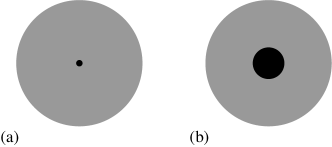
Figure 1: The static point singularity in the incompressible density of the polar-fluid droplet shown in (a) as a small black disc induces a puncture of radius (68) in the coordinate of the polar fluid droplet shown in (b) as a large disc. The polar-fluid droplet is shown as the grey disk in both (a) and (b).

III.5 Winding a quasi-particle around a quasi-vortex

We call $\tilde{j}^{\mu}$ and $\tilde{J}^{\mu\nu}$ the quasi-particle and quasi-vortex currents, respectively. We are first going to show how they can be related to a point-like defect such as the one represented by Eq. (69), to which the charge $e^{*}$ is associated, or the string-like defect such as the one represented by (70), to which the charge $s^{*}$ is associated. We will then derive the Berry phase induced when a quasi-particle excitation winds adiabatically $n$ times around a quasi-vortex excitation of the incompressible polar fluid with the BF action (39). In doing so, we are going to derive the quantization condition

$$\frac{g}{\hbar}\,\frac{e^{*}}{e^{\ }}\,\frac{s^{*}}{s^{\ }}\,n\in\mathbb{Z}.$$ (71)

To this end, we define the action of the fields $b$ and $d$ interacting with the quasi-particle and quasi-vortex currents by

$$S[b,d,\tilde{j},\tilde{J}]:=\int\mathrm{d}^{4}y\,\left(\mathcal{L}^{\,}_{\mathrm{BF}}+\mathcal{L}^{\,}_{e^{*}}[\tilde{j}]+\mathcal{L}^{\,}_{s^{*}}[\tilde{J}]\right),$$ (72a)

$$\mathcal{L}^{\,}_{\mathrm{BF}}:=\frac{g}{2\pi}\,\epsilon^{\mu\nu\lambda\sigma}\,b^{\,}_{\mu\nu}\,\partial^{\,}_{\lambda}d^{\,}_{\sigma},$$ (72b)

$$\mathcal{L}^{\,}_{e^{*}}[\tilde{j}^{\mu}]:=\frac{e^{*}}{e^{\ }}\,g\,d^{\,}_{\mu}\,\tilde{j}^{\mu},$$ (72c)

$$\mathcal{L}^{\,}_{s^{*}}[\tilde{J}^{\mu\nu}]:=\frac{s^{*}}{s^{\ }}\,g\,b^{\,}_{\mu\nu}\,\tilde{J}^{\mu\nu}.$$ (72d)

The quasi-particle and quasi-vortex currents $$\tilde{j}^{\mu} \tilde{J}^{\mu\nu} d^{\,}_{\mu} b^{\,}_{\mu\nu} \tilde{j}^{\mu} d^{\,}_{\mu} j^{\mu} A^{\,}_{\mu} e e^{*} e \tilde{J}^{\mu\nu} b^{\,}_{\mu\nu} J^{\mu\nu} B^{\,}_{\mu\nu} s s^{*} s$$ and couple to the fields and , respectively. The quasi-particle current couples to the dynamical field as the dynamical conserved current defined in Eq. (40) does to the external electromagnetic field through the electric charge in Eq. (48). Hence, the quasi-particle charge shares the same dimension as the electric charge , even though we allow for the possibility that they differ in value. Similarly, the quasi-vortex current couples to the dynamical field as the dynamical conserved current does to the external vortex field through the vortex charge in Eq. (48). Hence, the vortex charge shares the same dimension as , even though we allow for the possibility that they differ in value. The path integral

$$Z[\tilde{j},\tilde{J}]:= \,\int\mathcal{D}[d]\,\int\mathcal{D}[b]\,e^{+\mathrm{i}S[b,d,\tilde{j},\tilde{J}]/\hbar}$$

$$\equiv \,Z[0,0]\,e^{+\mathrm{i}S_{\textrm{eff}}[\tilde{j},\tilde{J}]/\hbar}$$ (72e)

defines the quantum theory with the action (72a) in the background of the sources $\tilde{j}^{\mu}$ and $\tilde{J}^{\mu\nu}$. Their mutual interactions are captured by the effective action $S^{\,}_{\mathrm{eff}}[\tilde{j},\tilde{J}]$ obtained after integrating out the $b$ and $d$ fields.

Since (72a) describes a quadratic action, we can obtain $S_{\textrm{eff}}[\tilde{j},\tilde{J}]$ by expressing the dependence of the fields $b$ and $d$ on the currents $\tilde{j}$ and $\tilde{J}$ via the equations of motion, which read

$$\frac{1}{2\pi}\,\epsilon^{\mu\nu\lambda\sigma}\,\partial^{\,}_{\nu}b^{\,}_{\lambda\sigma}=-\frac{e^{*}}{e^{\ }}\tilde{j}^{\mu}$$ (73)

(when varying with respect to $d^{\,}_{\mu}$ for $\mu=0,1,2,3$) and

$$\frac{1}{2\pi}\,\epsilon^{\mu\nu\lambda\sigma}\,\partial^{\,}_{\lambda}\,d^{\,}_{\sigma}=-\frac{s^{*}}{s^{\ }}\,\tilde{J}^{\mu\nu}$$ (74)

(when varying with respect to $b^{\mu\nu}$ for $\mu,\nu=0,1,2,3$).

Replacing the equations of motion (73) and (74) into (72a) yields

$$S^{\,}_{\mathrm{eff}}[\tilde{j},\tilde{J}]= \,\frac{e^{*}}{e^{\ }}\,g\,\int\,\mathrm{d}^{4}y\,\tilde{j}^{\mu}(y)\,d_{\mu}(y)$$

$$= \,-\frac{e^{*}}{e^{\ }}\,\frac{s^{*}}{s^{\ }}\,g\,\iint\mathrm{d}^{4}y\,\mathrm{d}^{4}y^{\prime}\,\times$$

$$\,\tilde{j}^{\mu}(y)\,\Big{(}\frac{1}{2\pi}\,\varepsilon^{\alpha\beta\lambda\mu}\,\partial_{\lambda}\Big{)}^{-1}(y-y^{\prime})\,\tilde{J}^{\alpha\beta}(y^{\prime}).$$ (75)

We define the static point defect

$$\tilde{j}^{0}(t,{\bm{y}}):=\delta(y^{\,}_{1})\,\delta(y^{\,}_{2})\,\delta(y^{\,}_{3}),\qquad\tilde{j}^{i}(t,{\bm{y}}):=0,$$ (76)

with $i=1,2,3$. According to Eq. (73), this is the source for the static field configuration

$$b^{\,}_{jk}(t,{\bm{y}})=-\frac{1}{4}\,\frac{e^{*}}{e^{\ }}\,\epsilon^{\,}_{jki}\,\frac{y^{\,}_{i}}{|{\bm{y}}|^{3}}$$ (77)

with $j,k=1,2,3$. For any closed surface $\Sigma$ that is the boundary of an open neighborhood that contains the origin $\bm{y}=0$ and is oriented outwards, Gauss law gives

$$\frac{1}{2\pi}\iint\limits_{\Sigma}\mathrm{d}y^{\,}_{j}\,\mathrm{d}y^{\,}_{k}\,b^{\,}_{jk}(t,\bm{y})=-\frac{e^{*}}{e^{\ }}.$$ (78)

Hence, the static point defect (76) binds the monopole-like field (77) with the monopole charge $-e^{*}/e$. We may then identify $-e^{*}/e$ with $q^{\,}_{e}$ in Eq. (69).

We define the static line defect

$$\tilde{J}^{03}(t,{\bm{y}}):=\delta(y^{\,}_{1})\,\delta(y^{\,}_{2}),\qquad\tilde{J}^{\mu\nu}(t,{\bm{y}}):=0$$ (79)

with $\mu=1,2,3$ and $\nu=0,1,2$. According to Eq. (74), this is the source for the static field configuration

$$d^{\,}_{1}(t,{\bm{y}})=+\frac{s^{*}}{s^{\ }}\,\frac{y^{\,}_{2}}{y^{2}_{1}+y^{2}_{2}},$$ (80a)

$$d^{\,}_{2}(t,{\bm{y}})=-\frac{s^{*}}{s^{\ }}\,\frac{y^{\,}_{1}}{y^{2}_{1}+y^{2}_{2}},$$ (80b)

$$d^{\,}_{3}(t,{\bm{y}})=0.$$ (80c)

For any closed curve $C^{\,}_{3}$ that winds around the axis $y^{\,}_{1}=y^{\,}_{2}=0$ counterclockwise,

$$\frac{1}{2\pi}\,\oint\limits_{C^{\,}_{3}}\mathrm{d}y^{\,}_{i}\,d^{\,}_{i}(t,\bm{y})=-\frac{s^{*}}{s^{\ }}.$$ (81)

Hence, the static line defect (79) binds the field (80) of an infinitesimal magnetic flux tube running along the $y^{\,}_{3}$ axis, i.e., a vortex field, of flux $-s^{*}/s$. We may then identify $-s^{*}/s$ with $q^{\,}_{s}$ in Eq. (70).

As a quasi-particle located at the time-dependent position ${\bm{r}}(t)$ and carrying the current

$$\tilde{j}^{\mu}_{\mathrm{adia}}(t,\bm{y}):=\begin{pmatrix}\delta\big{(}\bm{y}-\bm{r}(t)\big{)}\\ \frac{\mathrm{d}\bm{r}(t)}{\mathrm{d}t}\,\delta\big{(}\bm{y}-\bm{r}(t)\big{)}\end{pmatrix}$$ (82)

winds $n$ times adiabatically around the static quasi-vortex (79), it acquires the Berry phase defined by

$$e^{\mathrm{i}\Theta^{\,}_{\mathrm{B}}(n)/\hbar}:=e^{\mathrm{i}S^{\,}_{\mathrm{eff}}[\tilde{j}^{\,}_{\mathrm{adia}},\tilde{J}^{\,}_{\mathrm{adia}}]/\hbar}.$$ (83)

The computation of $\Theta^{\,}_{\mathrm{B}}$ gives

$$\Theta^{\,}_{\mathrm{B}}(n)= \,+\frac{e^{*}}{\hbar}\,\int\,\mathrm{d}^{4}y\,d^{\,}_{\mu}\,\tilde{j}^{\mu}_{\mathrm{adia}}$$

$$= \,-\frac{e^{*}}{\hbar}\,\int\mathrm{d}t\,\mathrm{d}^{3}{\bm{y}}\,\sum_{i=1,2}d^{\,}_{i}({\bm{y}})\,\tilde{j}^{\,}_{i}(t,{\bm{y}})$$

$$= \,-\frac{e^{*}}{\hbar}\,\int\mathrm{d}t\,\mathrm{d}^{3}{\bm{y}}\,\sum_{i=1,2}d^{\,}_{i}({\bm{y}})\,\frac{\mathrm{d}\,r^{\,}_{i}(t)}{\mathrm{d}\,t}\,\delta({\bm{y}}-{\bm{r}}(t))$$

$$= \,-\frac{e^{*}}{\hbar}\,\oint\limits_{C^{\,}_{3}}\,\mathrm{d}{\bm{r}}\cdot{\bm{d}}({\bm{r}})$$

$$= \,2\pi\,\frac{g}{\hbar}\,\frac{e^{*}}{e^{\ }}\,\frac{s^{*}}{s^{\ }}\,n.$$ (84)

We used Eq. (80) to deduce the second and last equalities.

If we demand that the quantum theory (72) is invariant under this adiabatic process, we must impose the quantization condition

$$\frac{g}{\hbar}\,\frac{e^{*}}{e^{\ }}\,\frac{s^{*}}{s^{\ }}\,n=m\in\mathbb{Z}.$$ (85)

We can use this quantization condition to find the minimum possible quantized charges in the theory. Physically we should demand that the Berry phase be an integer multiple of $2\pi$ whenever any quasiparticle winds once ($n=1$) around a fundamental vortex (of vorticity $s$). Similarly, the Berry phase associated with winding once a quasivortex around a fundamental charge (of charge $e$) must also be $2\pi$. This yields the conditions that the minimum fractional charges and vorticities are

$$\frac{e^{*}_{\rm min}}{e^{\ }}=\frac{\hbar}{g}\qquad{\rm and}\qquad\frac{s^{*}_{\rm min}}{s^{\ }}=\frac{\hbar}{g}\;.$$ (86)

This result is obtained using the minimum $m=1$.

IV Density operator algebra and the BF theory

In Sec. III.5, we extracted the braiding statistics of topological excitations in a polar fluid. We now deduce another important property of a polar fluid namely the algebra obeyed by the density operators of the polar fluid.

We recall that, in the two-dimensional quantum Hall fluid, the particle density operator obeys the GMP algebra (also known as the $W^{\,}_{\infty}$ algebra or the Fairlie-Fletcher-Zachos algebra). GMP1985 ; GMP1986 ; Fairlie1989a ; Fairlie1989b The GMP algebra plays an important role in the theory of the quantum Hall fluid. In the fractional quantum Hall effect, the GMP algebra can be used to construct, via a single-mode approximation, the magneto-roton excitation, a dispersing gapped charge-neutral collective excitation above the ground state. In the presence of a boundary (an edge), the GMP algebra describes the gapless edge excitations of quantum Hall liquid. (To be more precise, to describe edge states one needs to consider the GMP algebra with a central extension. The resulting algebra is called the $W^{\,}_{1+\infty}$ algebra.) Iso1992 ; Cappelli1993 ; Cappelli1995 ; Stone91 ; Martinez1993 ; Azuma94

In the polar fluid, it is natural to discuss, in addition to the particle density operator, a density operator associated to the vorticity, and commutation relations between these density operators. The BF Lagrangian (39) together with the identification of conserved densities (currents), Eqs. (40) and (41), suggest a non-vanishing commutator between these densities. (See below.) In this section, we discuss this issue with the help of a fermionic microscopic model – a free massive Dirac fermion in (3+1) dimensions. In the following, we will identify the density operators associated to the particle number and the vorticities within the Dirac model. Assuming the large mass gap, we will then project these density operators to the occupied bands and compute the commutation relations. Finally, we will make a comparison with the effective BF theory description.

IV.1 The density algebra in the massive Dirac fermion model

The Dirac Hamiltonian in question is given by

$$\hat{H}:=\sum_{\bm{k}}\hat{\Psi}^{{\dagger}}(\bm{k})\,\mathcal{H}(\bm{k})\,\hat{\Psi}(\bm{k}),$$ (87a)

where $$\hat{\Psi}(\bm{k})$$ is a four component fermion annihilation operator,

$$\hat{\Psi}(\bm{k}):=\left(\hat{\psi}^{\,}_{1}(\bm{k}),\hat{\psi}^{\,}_{2}(\bm{k}),\hat{\psi}^{\,}_{3}(\bm{k}),\hat{\psi}^{\,}_{4}(\bm{k})\right)^{\mathsf{T}},$$ (87b)

the momentum $$\bm{k}\in\mathbb{R}^{3} 4\times 4 \mathcal{H}$$, the single-particle Hermitian matrix takes the form

$$\mathcal{H}(\bm{k}):=\sum_{i=1}^{3}k^{\,}_{i}\,\alpha^{\,}_{i}+m\,\beta,$$ (87c)

and the gamma matrices are chosen to be in the Dirac representation

$$\alpha^{\,}_{i}\equiv\gamma^{\,}_{0}\,\gamma^{\,}_{i}:=\begin{pmatrix}0&\sigma^{\,}_{i}\\ \sigma^{\,}_{i}&0\end{pmatrix},\qquad\beta\equiv\gamma^{\,}_{0}:=\begin{pmatrix}\sigma^{\,}_{0}&0\\ 0&-\sigma^{\,}_{0}\end{pmatrix}.$$ (87d)

The spectrum of $\mathcal{H}$ consists of two doubly degenerate bands with the energy eigenvalues

$$\varepsilon^{\,}_{\pm}(\bm{k})=\pm\sqrt{\bm{k}^{2}+m^{2}}.$$ (88)

In the following, we assume the chemical potential such that the lowest two bands are fully occupied and the mass gap is large, much larger than any perturbations that we could add to the Dirac Hamiltonian. We are after the physics encoded by the lower bands. In particular, we seek the algebra obeyed by the charge and vortex density operators projected onto the lower bands. The charge-density operator in the Dirac model (before projection) is given by

$$\hat{\rho}:=\hat{\Psi}^{{\dagger}}\,\hat{\Psi}.$$ (89)

Once projected onto the two fully filled lowest bands, this operator should be compared with $\epsilon^{ijk}\partial^{\,}_{i}\hat{b}^{\,}_{jk}$ in the BF theory. As for the counterpart of $\epsilon^{ijk}\partial^{\,}_{j}\hat{d}^{\,}_{k}$, the spin-density operator is not appropriate as spin is not conserved due to the spin-orbit coupling. Instead, we consider the curl of the Dirac current,

$$\hat{\Lambda}^{i}:=\epsilon^{ijk}\partial^{\,}_{j}\left(\hat{\Psi}^{{\dagger}}\,\gamma^{0}\,\gamma_{k}\,\hat{\Psi}\right).$$ (90)

Assuming the mass $m$ to be “large”, we then evaluate the commutator for the charge and vortex density operators projected onto the lowest two occupied bands.

The comparison between the BF field theory and the non-interacting Dirac model is not expected to be perfect. To elaborate this point, we go momentarily back to two spatial dimensions. On the one hand, the GMP algebra is obtained for the charge-density operator projected onto the lowest Landau level, whereby the lowest Landau level has a uniform Berry curvature. On the other hand, the projected charge-density operator in two-dimensional Chern insulators do not obey the GMP algebra, since Chern bands have a non-uniform Berry curvature related as they are to the massive Dirac Hamiltonian in two-dimensional space. Parameswaran12 ; Goerbig12 ; Estienne12 ; Murthy12 ; Murthy11 ; Chamon12

While it may be possible to use three-dimensional Landau levels to make a better comparison with the density algebra derived from the BF theory, we will stick with the Dirac model for the sake of simplicity. A “trick” that we will use to improve the comparison is that we will focus on the region of the momentum space $|\bm{k}|/m\ll 0$ for which the Berry curvature is asymptotically uniform.

The projection onto the lowest bands can be done by first transforming the fermion operators $\hat{\psi}^{\,}_{\alpha}(\bm{k})$ with $\alpha=1,2,3,4$ into the eigenoperators $\hat{\chi}^{\,}_{a}(\bm{k})$ with $a=1,2,3,4$ of the Hamiltonian $\mathcal{H}(\bm{k})$ according to

$$\hat{\psi}^{{\dagger}}_{\alpha}(\bm{k})=\sum_{b=1}^{4}u^{b*}_{\alpha}(\bm{k})\,\hat{\chi}^{{\dagger}}_{b}(\bm{k}),$$ (91)

where $u^{b}_{\alpha}(\bm{k})$ are the components of the eigenfunctions (Bloch wave function) of $\mathcal{H}(\bm{k})$. In terms of $\hat{\chi}$ and $u$, the projected charge-density operator with momentum $\bm{q}$ is

$$\tilde{\rho}(\bm{q}):=\sum_{\bm{k}}\sum_{\alpha=1}^{4}\sum_{a,b=1}^{2}\left[u^{*}_{\alpha}(\bm{k})\,u^{\ }_{\alpha}(\bm{k}+\bm{q})\right]^{ab}\hat{\chi}^{{\dagger}}_{a}(\bm{k})\,\hat{\chi}^{\ }_{b}(\bm{k}+\bm{q}).$$ (92)

Projected operators acquire the $\tilde{}$ symbol instead of the $\hat{}$ symbol in order to imply the summation convention $\alpha=1,2,3,4$ on the Dirac labels, whereas the summation convention is restricted to the labels for the occupied Bloch bands, i.e., $a,b=1,2$. For $\bm{q}\to\bm{0}$, we expand $u(\bm{k}+\bm{q})$ to linear order in $\bm{q}$. Summing over the Dirac indices $\alpha=1,\cdots,4$ gives

$$\tilde{\rho}(\bm{q})\approx\sum_{\bm{k}}\sum_{a,b=1}^{2}\left[1+q^{i}\,A^{\,}_{i}(\bm{k})\right]^{ab}\hat{\chi}^{{\dagger}}_{a}(\bm{k})\,\hat{\chi}^{\ }_{b}(\bm{k}+\bm{q}),$$ (93a)

where

$$A^{i}(\bm{k}):=\sum_{\alpha=1}^{4}u^{*}_{\alpha}(\bm{k})\,(\partial^{i}u^{\,}_{\alpha})(\bm{k}),\qquad i=1,2,3,$$ (93b)

is a non-Abelian U(2) Berry connection and the summation convention over the index $$i=1,2,3 \bm{q} \bm{A}^{\,}_{1} \bm{A}^{\,}_{2} (3+1) i=1,2,3$$ that labels the components of the three-dimensional wave number is implied. This non-Abelian U(2) Berry connection can be decomposed into a U(1) part () and an SU(2) part (). For the massive Dirac Hamiltonian in -dimensional space and time, their components labeled by are

$$(A^{i}_{1})^{ab}(\bm{k})=\frac{-k^{i}}{2k^{\,}_{0}\,(k^{\,}_{0}+m)}\,\delta^{ab},$$ (93c)

and

$$(A^{i}_{2})^{ab}(\bm{k})=\frac{\mathrm{i}\epsilon^{\,}_{ijk}\,(\sigma^{j})^{ab}\,k^{k}}{2k^{\,}_{0}\,(k^{\,}_{0}+m)},$$ (93d)

respectively, where $k^{\,}_{0}:=\sqrt{\bm{k}^{2}+m^{2}}$.

Similarly, the components labeled by the index $i=1,2,3$ of the spin-density operator are defined to be

$$\hat{\Lambda}^{i}(\bm{q}):=\epsilon^{ijk}\,\partial^{j}j^{k}(\bm{q}),$$ (94a)

where $$\hat{j}^{i}(\bm{q})$$ is the Dirac 3-current operator

$$\hat{j}^{i}(\bm{q}):=\sum_{\bm{k}}\hat{\bar{\Psi}}(\bm{k})\gamma^{i}\hat{\Psi}(\bm{k}+\bm{q}).$$ (94b)

After projecting onto the lowest two occupied bands, the spin-density operator takes the form

$$\tilde{\Lambda}^{i}(\bm{q}):= \,\sum_{\bm{k}}\mathrm{i}\epsilon^{ijk}\,q^{\,}_{j}\left[u^{*}_{\alpha}\left(\gamma^{0}\gamma^{k}\right)^{\alpha\beta}u^{\,}_{\beta}(\bm{k}+\bm{q})\right]^{ab}$$

$$\,\times\hat{\chi}^{{\dagger}}_{a}(\bm{k})\,\hat{\chi}^{\,}_{b}(\bm{k}+\bm{q}).$$ (95)

To lowest leading order in a gradiant expansion of the Bloch states $a,b=1,2$,

$$\tilde{\Lambda}^{i}(\bm{q})\approx \,\sum_{\bm{k}}\mathrm{i}\epsilon^{ijk}\,q^{\,}_{j}\,\left[B^{\,}_{0,k}(\bm{k})+q^{l}\,(B_{1,k}^{l}(\bm{k})+B_{2,k}^{l}(\bm{k}))\right]^{ab}$$

$$\,\times\hat{\chi}^{{\dagger}}_{a}(\bm{k})\,\hat{\chi}_{b}(\bm{k}+\bm{q}).$$ (96a)

For the massive Dirac Hamiltonian in $$(3+1)$$ dimensional space and time,

$$B^{\,}_{0,i}(\bm{k})=\frac{k^{\,}_{i}}{k^{\,}_{0}}\,\delta^{ab},$$ (96b)

$$B^{i}_{1,j}(\bm{k})=\frac{-k^{i}\,k_{j}\,m}{2\,k^{3}_{0}\,(k^{\,}_{0}+m)}\,\delta^{ab},$$ (96c)

$$B^{i}_{2,j}(\bm{k})=\mathrm{i}\left[\epsilon^{\,}_{ljl}\,\frac{k^{i}\,k^{l}}{k^{\,}_{0}}+\epsilon^{\,}_{jil}(k^{\,}_{0}+m)\right]\,(\sigma^{l})^{ab}.$$ (96d)

Again, we have explicitly kept terms that vanish by contraction with an antisymmetric tensor.

If we only consider the leading order term in an expansion in powers of the components of $q^{\,}_{1}$ and $q^{\,}_{2}$, we obtain

$$\left[\tilde{\rho}(\bm{q}^{\,}_{1}),\tilde{j}^{\,}_{i}(\bm{q}^{\,}_{2})\right]= \,q^{j}_{1}\sum_{\bm{k}}\left[\partial^{\,}_{j}B^{\,}_{0i}\right]^{ab}\hat{\chi}^{{\dagger}}_{a}(\bm{k})\,\hat{\chi}^{\,}_{b}(\bm{k}+\bm{q}^{\,}_{1}+\bm{q}^{\,}_{2})$$

$$\,+\cdots$$ (97)

and

$$\left[\tilde{\rho}(\bm{q}^{\,}_{1}),\tilde{\Lambda}^{\,}_{i}(\bm{q}^{\,}_{2})\right]= \,\mathrm{i}\epsilon^{\,}_{ijk}\,q^{l}_{1}\,q^{j}_{2}\sum_{\bm{k}}\left[\partial^{\,}_{l}B^{k}_{0}(\bm{k})\right]^{ab}$$

$$\,\times\hat{\chi}^{{\dagger}}_{a}(\bm{k})\,\hat{\chi}^{\,}_{b}(\bm{k}+\bm{q}^{\,}_{1}+\bm{q}^{\,}_{2})+\cdots.$$ (98)

When $|\bm{k}|\ll m$, we arrive at

$$\left[\tilde{\rho}(\bm{q}^{\,}_{1}),\tilde{\Lambda}^{\,}_{i}(\bm{q}^{\,}_{2})\right] =\mathrm{i}\epsilon^{\,}_{ijk}\,\frac{q^{k}_{1}\,q^{j}_{2}}{m}\tilde{\rho}(\bm{q}^{\,}_{1}+\bm{q}^{\,}_{2})+\cdots.$$ (99)

This is an analogue of the GMP algebra.

We now compare the commutator (99) derived from the massive Dirac model with the corresponding commutator in the BF theory. We begin with the BF Lagrangian density (39) in the temporal gauge

$$d^{\,}_{0}=b^{\,}_{0i}=0.$$ (100a)

It is given by

$$\mathcal{L}=\frac{g}{2\pi}\,\epsilon^{\,}_{ijk}\,\dot{d}^{\,}_{i}\,b^{\,}_{jk}=g\,\dot{d}^{\,}_{i}\,B^{i},$$ (100b)

where we have defined

$$B^{i}:=\frac{1}{2\pi}\,\epsilon^{ijk}\,b^{\,}_{jk}\equiv\frac{1}{2\pi}\,\epsilon^{\,}_{ijk}\,b^{\,}_{jk}.$$ (100c)

Canonical quantization for the canonical pair $d^{\,}_{i}$ and $g\,B^{i}$ implies the equal-time commutation relation

$$\left[\hat{d}^{\,}_{i}(\bm{x}),\hat{B}^{j}(\bm{y})\right]=\mathrm{i}g^{-1}\,\delta(\bm{x}-\bm{y})\,\delta^{j}_{\ i}$$ (101)

for $i,j=1,\cdots,3$. Recalling the definitions of the conserved currents, Eqs. (40) and (41), the commutator (101) resembles the commutator (99), i.e., the presence of the factor $\epsilon^{\,}_{ijk}\,q^{k}_{1}\,q^{j}_{2}$, although there is no particle number density operator on the right-hand side of the commutator (101).

In fact, the absence of the density operator on the right-hand side of of Eq. (101) is anticipated (see below), and the comparison between the commutators derived from the microscopic model and from the effective field theory is not expected to be complete. Within the BF theory description, the particle density is completely frozen in the bulk and does not fluctuate. Hence, the density operator on the right-hand side of the commutator (101) is “invisible”. This situation is completely analogous to the Chern-Simons description of the quantum Hall fluid. In the Chern-Simons description of quantum Hall fluid, the only collective charge fluctuations described by the Chern-Simons theory are edge excitations (apart from the point-like quasiparticle excitations in the bulk). Hence, one can not derive the GMP algebra in the bulk from the Chern-Simons theory. Nevertheless, the description of edge excitations derived from the Chern-Simons theory is consistent with the edge excitations derived from the GMP algebra. Iso1992 ; Cappelli1993 ; Cappelli1995 ; Stone91 ; Martinez1993 ; Azuma94

V Discussion

We have formulated a hydrodynamic description of gapped topological electron fluid in term of the BF effective field theory. Just as fluid dynamics is an efficient description of a collection of macroscopic number of interacting particles, the hydrodynamic BF field theory allows us to describe incompressible electron liquid beyond single particle physics. From the BF theory, we have extracted statistical information of defects in the polar fluid.

We close with two comments. (i) In the last section, we have linked the hydrodynamic BF theory to the algebra of densities in the polar fluid. The hydrodynamic BF theory may be derived, alternatively, by using functional bosonization techniques. In the functional bosonization approach, one derives an effective action that encodes the low-energy and long-wavelength properties of conserved quantities (hydrodynamic modes) for a given microscopic model. For example, descriptions of topological insulators in terms of effective field theories have been derived by bosonizing the charge $U(1)$ degrees of freedom in topological insulators. Chan12 In the polar fluid, we are concerned with two kinds of densities, the charge and vorticity densities. A functional bosonization can be adopted to take into account both kinds of densities. unpublished

(ii) The purpose of the present paper was to derive a hydrodynamic description of incompressible topological fluid with a few basic assumptions. As such, hydrodynamic field theories can describe both bosonic and fermionic lattice models, e.g., bosonic and fermionic topological insulators, at low energies and long wavelengths. (See, e.g., Refs. Vishwanath2013, ; Kapustin2014, and YeGu2014, for discussions of bosonic topological insulators and their descriptions in terms of BF theories). By construction, hydrodynamic field theories are written in terms of bosonic degrees of freedom (describing conserved hydrodynamic modes). Hence, the distinction between the cases when the underlying particles obey bosonic or fermionic statistics has to be encoded in a rather subtle way. For example, in the Chern-Simons theory of the fractional quantum fluid, the distinction between bosonic/fermionic statisctic of fundamental particles manifests itself as eveness/oddness of the level of the Chern-Simons term. In our description of three-dimensional topological incompressible fluid, we expect that the bosonic/fermionic statistics is encoded by the periodicity of the $\theta$ angle in the axion term; for bosonic (fermionic) underlying particles, the periodicity is $4\pi$ ($2\pi$).

References

• (1) The Quantum Hall Effect, edited by R. E. Prange and S. M. Girvin (Springer, New York, 1987).
• (2) S. Bahcall and L. Susskind, Int. J. Mod. Phys. B 5, 2735-2750 (1991).
• (3) L. Susskind, arXiv:hep-th/0101029.
• (4) R. Jackiw, V. P. Nair, S.-Y. Pi, and A. P. Polychronakos, J. Phys. A: Math. Gen. 37, R327 R432 (2004).
• (5) M. Z. Hasan and C. L. Kane, Rev. Mod. Phys. 82, 3045 (2010).
• (6) X.-L. Qi and S.-C. Zhang, Rev. Mod. Phys. 83, 1057 (2011).
• (7) A. P. Schnyder, S. Ryu, A. Furusaki, and A. W. W. Ludwig, Phys. Rev. B 78, 195125 (2008).
• (8) A. Kitaev, AIP Conf. Proc. 1134, 22 (2009);arXiv:0901.2686.
• (9) S. Ryu, A. P. Schnyder, A. Furusaki, and A. W. W. Ludwig, New J. Phys. 12, 065010 (2010).
• (10) M. Levin and A. Stern, Phys. Rev. Lett. 103, 196803 (2009).
• (11) T. Neupert, L. Santos, S. Ryu, C. Chamon ans C. Mudry, Phys. Rev. B 84, 165107 (2011).
• (12) L. Santos, T. Neupert, S. Ryu, C. Chamon ans C. Mudry, Phys. Rev. B 84, 165138 (2011).
• (13) X. Chen, Z.-C. Gu, Z.-X. Liu, and X.-G. Wen, Science 338, 1604 (2012).
• (14) Y.-M. Lu and A. Vishwanath, Phys. Rev. B 86, 125119 (2012).
• (15) A. Vishwanath and T. Senthil, Phys. Rev. X 3, 011016 (2013).
• (16) C. Wang, A. Potter, and T. Senthil, Science 343, 6171 (2014).
• (17) M. Blau and G. Thompson, Ann. Phys. 205, 130 (1991).
• (18) M. Bergeron, G. W. Semenoff, and R. J. Szabo, Nucl. Phys. B 437, 695 (1995).
• (19) R. J. Szabo, Nucl. Phys. B 531, 525 (1998).
• (20) T. H. Hansson, V. Oganesyan, and S. L. Sondhi, Ann. Phys. 313, 497 (2004).
• (21) G. Y. Cho and J. E. Moore, Ann. Phys. 326, 1515 (2011).
• (22) E. Witten, Phys. Lett. B 86, 283 (1979).
• (23) X. L. Qi, T. L. Hughes, and S.-C. Zhang, Phys. Rev. B 78, 195424 (2008); Phys. Rev. B 81, 159901(E) (2010).
• (24) G. Rosenberg and M. Franz, Phys. Rev. B 82, 035105 (2010).
• (25) S. M. Girvin, A. H. MacDonald, and P. M. Platzman, Phys. Rev. Lett. 54, 581 (1985).
• (26) S. M. Girvin, A. H. MacDonald, and P. M. Platzman, Phys. Rev. B 33, 2481 (1986).
• (27) D. B. Fairlie, P. Fletcher, and Cosmas K. Zachos, Phys. Lett. B 218, 203 (1989).
• (28) D. B. Fairlie and Cosmas K. Zachos, Phys. Lett. B 224, 101 (1989).
• (29) S. Iso, D. Karabali, and B. Sakita, Phys. Lett. B 296, 143 (1992).
• (30) A. Cappelli, C. Trugenberger, and G. Zemba, Nucl. Phys. B 396, 465 (1993).
• (31) A. Cappelli, C. Trugenberger and G. Zemba, Nucl.  Phys. B, 448, (1995).
• (32) M. Stone, Int.  J.   Mod.  Phys.  B, 05, 509 (1991).
• (33) J. Martinez and M. Stone, Int. J. Mod. Phys. B 7, 4389 (1993).
• (34) H. Azuma, Prog. Theor. Phys. 92, 293 (1994).
• (35) A. Chan, T. Hughes, S. Ryu, and E. Fradkin, Phys. Rev. B 87, 085132 (2013).
• (36) A. Tiwari, X. Chen, T. Neupert, L. H. Santos, S. Ryu, C. Chamon, and C. Mudry, unpublished.
• (37) S. Parameswaran, R. Roy, and S. Sondhi, Phys. Rev. B 85, 241308(R) (2012).
• (38) M. O. Goerbig, Eur. Phys. Journal B 85, 14 (2012).
• (39) B. Estienne, N. Regnault, and B. A. Bernevig, Phys. Rev. B 86, 241104(R) (2012).
• (40) G. Murthy and R. Shankar, Phys. Rev. B 86, 195146 (2012).
• (41) G. Murthy and R. Shankar, arXiv:1108.5501.
• (42) Claudio Chamon and Christopher Mudry, Phys. Rev. B 86, 195125 (2012).
• (43) A. Kapustin, arXiv:1403.1467 (unpublished).
• (44) P. Ye and Z. -C. Gu, arXiv:1410.2594 (unpublished).