The stellar-to-halo mass relation of local galaxies segregates by color

Abstract

By means of a statistical approach that combines different semi-empirical methods of galaxy-halo connection, we derive the stellar-to-halo mass relations, SHMR, of local blue and red central galaxies separately. We also constrain the fraction of halos hosting blue/red central galaxies and the occupation statistics of blue and red satellites as a function of halo mass, $M_{\rm h}$. For the observational input, we use the blue and red central/satellite galaxy stellar mass functions and two-point correlation functions in the stellar mass range of $9<$log($M_{*}$/M_⊙)$<12$. We find that: (1) the SHMR of central galaxies is segregated by color, with blue centrals having a SHMR above the one of red centrals; at log($M_{\rm h}$/M_⊙)$\sim 12$, the $M_{*}$-to-$M_{\rm h}$ ratio of the blue centrals is $\approx 0.05$, which is $\sim 1.7$ times larger than the value of red centrals. (2) The constrained scatters around the SHMRs of red and blue centrals are $\approx 0.14$ and $\approx 0.11$ dex, respectively. The scatter of the average SHMR of all central galaxies changes from $\sim 0.20$ dex to $\sim 0.14$ dex in the $11.3<$log($M_{\rm h}$/M_⊙)$<15$ range. (3) The fraction of halos hosting blue centrals at $\mbox{$M_{\rm h}$}=10^{11}$ M_⊙ is 87%, but at $2\times 10^{12}$ M_⊙ decays to $\sim 20\%$, approaching to a few per cents at higher masses. The characteristic mass at which this fraction is the same for blue and red galaxies is $\mbox{$M_{\rm h}$}\approx 7\times 10^{11}$ M_⊙. Our results suggest that the SHMR of central galaxies at large masses is shaped by mass quenching. At low masses, processes that delay star formation without invoking too strong supernova-driven outflows could explain the high $M_{*}$-to-$M_{\rm h}$ ratios of blue centrals as compared to those of the scarce red centrals.

1. Introduction

The current paradigm of galaxy formation and evolution has its theoretical background in the $\Lambda$ cold dark matter ($\Lambda$CDM) cosmological model. In this paradigm, the backbone of galaxy formation are the gravitationally bound CDM structures (halos) in the cosmic web. The statistical properties and mass assembling of CDM halos have been calculated with great detail, mainly by means of large N-body cosmological simulations (for a recent review, see Knebe et al., 2013). Of particular relevance is the halo mass function (HMF), the number of halos of a given mass per unit of comoving volume, which can be divided into halos not contained inside larger ones (distinct) and subhalos. In the understanding that halos and subhalos are populated respectively by central and satellite galaxies, the galaxy-(sub)halo connection can be stablished at a statistical level by using observed galaxy distributions such as the galaxy stellar mass function (GSMF), the two-point correlation function, and the satellite conditional stellar mass functions. The resulting semi-empirical galaxy-(sub)halo connection provides a powerful tool to constrain galaxy evolution models as well as the properties of galaxies as a function of scale and environment (Mo, van den Bosch & White, 2010).

In recent years, several statistical approaches have emerged for connecting galaxies to their CDM halos. Among the simplest ones is the so-called (sub)halo abundance matching technique (SHAM). The SHAM consists in assigning by rank a galaxy stellar mass, $M_{*}$, (or luminosity) to a host dark matter halo of mass $M_{\rm h}$ by matching their corresponding cumulative number densities. (e.g., Kravtsov et al., 2004; Vale & Ostriker, 2004, 2008; Conroy, Wechsler & Kravtsov, 2006; Shankar et al., 2006; Behroozi, Conroy & Wechsler, 2010; Guo et al., 2010; Rodríguez-Puebla, Drory & Avila-Reese, 2012; Papastergis et al., 2012; Hearin et al., 2013; Behroozi, Wechsler & Conroy, 2013). As a result from this matching, one obtains the total stellar-to-halo mass relation (SHMR). Usually the SHMR is assumed to be identical both for central and for satellite galaxies. However, recent studies (Neistein et al., 2011; Yang et al., 2012; Rodríguez-Puebla, Drory & Avila-Reese, 2012; Reddick et al., 2013) have questioned this assumption, which has intrinsic issues for satellite galaxies and implicitly assumes that their SHMR does not evolve as a function of redshift and they have the same evolution trajectories as subhalos (e.g., no orphan satellite galaxies, etc.). In addition to the SHAM, there are other semi-empirical approaches for constraining the distribution of central and satellite galaxies inside the halos, such as the halo occupation distribution (HOD) model (e.g., Jing, Mo & Börner, 1998; Berlind & Weinberg, 2002; Cooray & Sheth, 2002; Zehavi et al., 2005; Abbas & Sheth, 2006; Foucaud et al., 2010; Zehavi et al., 2011; Watson, Berlind & Zentner, 2011; Wake, Franx & van Dokkum, 2012; Leauthaud et al., 2012), and the closely related conditional stellar mass (or luminosity) function model (Yang, Mo & van den Bosch, 2003; van den Bosch, Yang & Mo, 2003; Cooray, 2006; Yang et al., 2007; van den Bosch et al., 2007; Yang, Mo & van den Bosch, 2009a; Yang et al., 2012, hereafter Y12). These approaches use the observed 2PCF and/or galaxy group catalogs for constraining the central/satellite galaxy distributions, respectively. By combining thus constrained survived satellite population together with accreted ones predicted using the halo merger histories, one can model the evolution of these galaxies satellite galaxies and their contribution to the evolution of central galaxies (e.g., Yang, Mo & van den Bosch, 2009b; Yang et al., 2012, 2013)

By combining the above mentioned semi-empirical approaches, Rodríguez-Puebla, Avila-Reese & Drory (2013, hereafter RAD13) were able to derive separately the SHMR of local central galaxies–distinct halos and satellite galaxies–subhalos as well as several occupation distributions (for closely related works see also Yang, Mo & van den Bosch, 2009b; Neistein et al., 2011; Reddick et al., 2013; Watson & Conroy, 2013). Actually, the total, central, and satellite SHMRs have intrinsic scatters related to the stochastic halo assembly and the complex processes of galaxy evolution. In most of the previous works, the intrinsic scatter around the median SHMR has been assumed as random as well as constant as a function of halo mass. Previous works have measured or constrained the intrinsic scatter around the SHMR finding typically that this is small, $\sim 0.15-0.20$ dex in log$M_{*}$( c.f. Mandelbaum et al., 2006; Yang, Mo & van den Bosch, 2008; More et al., 2011; Skibba et al., 2011; Leauthaud et al., 2012; Reddick et al., 2013; Kravtsov, Vikhlinin & Meshscheryakov, 2014, RAD13).

A natural next step in understanding the link between galaxies and halos is to explore what galaxy properties are related to the shape and scatter of the SHMR. The fact that for a given $M_{\rm h}$, there are galaxies more or less massive than the mean $M_{*}$ corresponding to this $M_{\rm h}$, certainly tells us something about the galaxy evolution process, in particular if these deviations correlate with a given galaxy property. In the era of big galaxy surveys, galaxy color is one of the most immediate observational properties reported in these surveys. It is well known that the color distribution of galaxies is bimodal (c.f. Baldry et al., 2004; Brinchmann et al., 2004; Weinmann et al., 2006; van den Bosch et al., 2008). This color bimodality strongly correlates with mass and in less degree with environment (Blanton & Moustakas, 2009, and more references therein; see also Peng & et al., 2010). The color is a fundamental property of galaxies related mainly to their star formation (SF) history, and it correlates in more or less degree with other galaxy properties such as the specific star formation (SF) rate and morphology.

Here, we pose the question whether the SHMR of local blue and red central galaxies are similar or not, and therefore, whether the scatter around the total SHMR of central galaxies is segregated by color. In order to tackle this question as general as possible, the assumption that the distribution of $M_{*}$ for a given $M_{\rm h}$ is given by a unique random (lognormal) function should be relaxed; instead we will consider that blue and red galaxies have their own distributions (intrinsic scatters). If both distributions, after being constrained with observations, are statistically similar, then galaxy color is not the responsible for shaping the intrinsic scatter of the SHMR.

Researchers have attempted to constrain the galaxy-halo connection for local and high-redshift galaxies separated by color or morphology using direct methods, namely the galaxy-galaxy weak lensing (Mandelbaum et al., 2006; van Uitert et al., 2011; Velander et al., 2014; Hudson et al., 2013) and the satellite kinematics (Conroy et al., 2007; More et al., 2011; Wojtak & Mamon, 2013) In order to attain the necessary signal-to-noise ratio, the current method requires stacking the data from large surveys, and even then uncertainties are yet large. Despite the large uncertainty and limited mass range, the obtained results suggest that the SHMR of blue and red (late- and early-type) galaxies could be different. Additionally, in a combined analysis of galaxy clustering and galaxy-galaxy weak lensing, Tinker et al. (2013) also concluded that the SHMR of passive and active galaxies are different in the COSMOS field at $z=[0.2,1.0]$ (see also Hartley et al., 2013).

By using a semi-empirical model that generalizes the one presented in RAD13, here we determine statistically the local SHMR of blue and red central galaxies separately, in the mass range of $\mbox{$M_{*}$}\approx 10^{9}-10^{12}$ M_⊙, as well as their corresponding blue and red satellite populations. In addition, we constrain separately the scatters around the SHMRs of blue and red centrals, and the scatter around the (bimodal) distribution of the (average) SHMR of all central galaxies. The semi-empirical study of the SHMR of central blue/red galaxies will allow us to understand what mechanisms carved the SHMR and will shed light into the relevant galaxy evolutionary processes as a function of scale and environment. Additionally, an important aspect of the SHMR of blue and red central galaxies is whether they are consistent with observabed galaxy correlations as the Tully-Fisher and Faber-Jackson relations. In the present paper we present our semi-empirical model in detail and the main results regarding the SHMR of central blue and red galaxies. In future works, we will use the model results for exploring the mentioned above aspects. In addition, we will also explore the properties of halos hosting blue and red central galaxies.

The plan for this paper is as follows. In Section 2, we describe our semi-empirical approach, as well as the required input, key assumptions, and the statistical procedure for constraining the model parameters. In Section 3, we describe the observational data to be used. Our main results are presented in Section 4. In Section 5, we discuss on the robustness and the interpretation of our results. In the same Section, we also compare the results obtained here with previous studies. Finally, a summary and the conclusion are presented in Section 6.

Unless otherwise stated, all of our calculations are based on a flat $\Lambda$CDM cosmology with $\Omega_{\Lambda}=0.73$, $h=0.7$ and $\sigma_{8}=0.84$.

2. The semi-empirical model

In this Section we describe the semi-empirical model developed for connecting blue and red central galaxies to their host dark matter halos, and for obtaining the occupational statistics of blue and red satellite galaxies. The model allows us to relate the central and satellite GSMFs and the projected two-point correlation functions (2PCFs), as well as their decompositions into blue and red galaxies, to the theoretical $\Lambda$CDM halo mass function. By means of this model, from the observed total, central and satellite GSMFs and the projected 2PCFs, in all the cases decomposed into blue and red populations, we can constrain: the stellar-to-halo mass relations, SHMRs, of blue, red and all (average) central galaxies, the fraction of halos hosting blue and red central galaxies, and the satellite blue/red conditional stellar mass functions (CSMFs) as a function of host halo or central galaxy stellar mass. The statistical model presented here combines the SHAM, HOD model and CSMF formalism as presented in RAD13. In order to include separately populations of blue and red galaxies, one requires some additional ingredients described as follows:

• For connecting blue and red central galaxies to their host dark matter halos, we introduce the conditional probability distribution functions that a distinct halo of mass $M_{\rm h}$ hosts either a blue or red central galaxy in the stellar mass bin $\mbox{$M_{*}$}\pm d\mbox{$M_{*}$}/2$, denoted by $P_{c,b}(\mbox{$M_{*}$}|\mbox{$M_{\rm h}$})$ and $P_{c,r}(\mbox{$M_{*}$}|\mbox{$M_{\rm h}$})$, respectively. As a result, these distributions contain information about the SHMR (mean and scatter) of blue and red central galaxies, $M_{*,b}$($M_{\rm h}$) and $M_{*,r}$($M_{\rm h}$), respectively.

• In order to derive $M_{*,b}$($M_{\rm h}$) and $M_{*,r}$($M_{\rm h}$), the fraction of halos hosting blue and red central galaxies should be known. Motivated by observational results, we introduce a parametric function for these fractions that will be constrained with the observational input.

• To model the occupational numbers of blue and red satellites, we use observationally-motivated parametric functions for the blue and red satellite CSMFs.

In Fig. 1, we present a schematic table that summarizes the main idea behind our model. We also indicate the kind of observational data we use for constraining the model parameters as well as our model predictions. Note that relevant (sub)sections and equations are also indicated. In the following we describe our model in more detail as well as the observational data employed to constrain the model parameters.

Those readers interested only on the results obtained with our model and their implications may prefer to skip to Section 4.

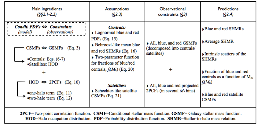
Figure 1.— Summary of our model, its main assumptions, observational data required for constraining it, and the main predictions from this model. The relevant (sub)sections and equations are indicated.

2.1. Modeling the Galaxy Stellar Mass Function

One can express the total GSMF by separating the population of galaxies into central and satellites:

$$\mbox{$\phi_{g,t}$}(\mbox{$M_{*}$})=\mbox{$\phi_{g_{c},t}$}(\mbox{$M_{*}$})+\mbox{$\phi_{g_{s,t}}$}(\mbox{$M_{*}$}),$$ (1)

each of which can be subdivided into blue and red galaxy populations, i.e.,

$$\mbox{$\phi_{g,t}$}(\mbox{$M_{*}$})=[\mbox{$\phi_{g_{c},b}$}(\mbox{$M_{*}$})+\mbox{$\phi_{g_{c},r}$}(\mbox{$M_{*}$})]+[\mbox{$\phi_{g_{s,b}}$}(\mbox{$M_{*}$})+\mbox{$\phi_{g_{s,r}}$}(\mbox{$M_{*}$})].$$ (2)

By defining the CSMF, $\Phi_{i,j}(\mbox{$M_{*}$}|\mbox{$M_{\rm h}$})$, as the mean number of ‘$i$ type’ ($i=$central or satellite) galaxies of a ‘$j$ color’ ($j=$blue or red) at the mass bin $\mbox{$M_{*}$}\pm d\mbox{$M_{*}$}/2$, one can write each component of the GSMFs in the following form:

$$\mbox{$\phi_{g_{i,j}}$}(\mbox{$M_{*}$})=\int\mbox{$\Phi_{i,j}(\mbox{$M_{*}$}|\mbox{$M_{\rm h}$})$}\mbox{$\phi_{h}$}(\mbox{$M_{\rm h}$})d\mbox{$M_{\rm h}$},$$ (3)

where $\phi_{h}$ is the distinct halo mass function. Thus, the mean cumulative number density galaxies of type ‘$i$’ and color ‘$j$’ can be written as

$$\mbox{$n_{g_{i},j}$}(>\mbox{$M_{*}$})=\int\mbox{$\langle N_{i,j}(>\mbox{$M_{*}$}|\mbox{$M_{\rm h}$})\rangle$}\mbox{$\phi_{h}$}(\mbox{$M_{\rm h}$})d\mbox{$M_{\rm h}$},$$ (4)

where,

$$\mbox{$\langle N_{i,j}(>\mbox{$M_{*}$}|\mbox{$M_{\rm h}$})\rangle$}=\int_{M_{*}}^{\infty}\mbox{$\Phi_{i,j}(M_{*}^{\prime}|\mbox{$M_{\rm h}$})$}dM_{*}^{\prime},$$ (5)

is the mean cumulative number of galaxies of the type ‘$i$’ and color ‘$j$’ with stellar masses greater than $M_{*}$ residing in a halo of mass $M_{\rm h}$. Observe that once the CSMFs $\Phi_{i,j}(\mbox{$M_{*}$}|\mbox{$M_{\rm h}$})$ are given, Eqs. (3-5) are totally defined. Therefore, the key ingredients in our model are the conditional mass functions $\Phi_{i,j}(\mbox{$M_{*}$}|\mbox{$M_{\rm h}$})$.

2.1.1 Central Galaxies

In the context of the SHAM, the connection between the total central GSMF, $\phi_{g_{c},t}$($M_{*}$), and the distinct halo mass function, $\phi_{h}$($M_{\rm h}$), arises naturally by assuming a probability distribution function, denoted by $P_{c,t}(\mbox{$M_{*}$}|\mbox{$M_{\rm h}$})$, that a distinct halo of mass $M_{\rm h}$ hosts a central galaxy in the stellar mass bin $\mbox{$M_{*}$}\pm d\mbox{$M_{*}$}/2$ (see Introduction for references). As a result of this connection, the mean SHMR of central galaxies, $M_{*}$($M_{\rm h}$), can be constrained. In the case that the GSMF is divided into different populations, the above idea can be extended in order to connect the different galaxy populations to their host dark matter halos. For blue and red galaxies, one can introduce the conditional probability distribution functions $P_{c,b}(\mbox{$M_{*}$}|\mbox{$M_{\rm h}$})$ and $P_{c,r}(\mbox{$M_{*}$}|\mbox{$M_{\rm h}$})$ to establish the statistical connection between the “blue”, $\phi_{h,b}$, and “red”, $\phi_{h,r}$, distinct halo mass functions and the GSMFs of blue and red centrals, $\phi_{g_{c},b}$ and $\phi_{g_{c},r}$, respectively. As above, the mean relations $M_{*,b}$($M_{\rm h}$) and $M_{*,r}$($M_{\rm h}$) are the result of this connection.

In terms of the CSMF formalism, one can specify the central CSMF as the sum of the blue and a red components,

$$\mbox{$\Phi_{c,t}(\mbox{$M_{*}$}|\mbox{$M_{\rm h}$})$}=\mbox{$\Phi_{c,b}(\mbox{$M_{*}$}|\mbox{$M_{\rm h}$})$}+\mbox{$\Phi_{c,r}(\mbox{$M_{*}$}|\mbox{$M_{\rm h}$})$},$$ (6)

where the CSMF of blue and red central galaxies are given by

$$\mbox{$\Phi_{c,j}(\mbox{$M_{*}$}|\mbox{$M_{\rm h}$})$}=\mbox{$f_{j}$}(\mbox{$M_{\rm h}$})\times\mbox{$P_{c,j}(\mbox{$M_{*}$}|\mbox{$M_{\rm h}$})$}.$$ (7)

As above, the subscript $j$ refers either to red (r) or blue (b) central galaxies, and $\mbox{$f_{j}$}(\mbox{$M_{\rm h}$})$ is the fraction of halos hosting central galaxies of color $j$. Notice that for all central galaxies, the CSMF is simply given by $\mbox{$\Phi_{c,t}(\mbox{$M_{*}$}|\mbox{$M_{\rm h}$})$}=\mbox{$P_{c,t}(\mbox{$M_{*}$}|\mbox{$M_{\rm h}$})$}$.

By inserting Eq. (7) into Eq. (6) one can obtain the relation between the probability distribution functions $P_{c,t}(\mbox{$M_{*}$}|\mbox{$M_{\rm h}$})$, $P_{c,b}(\mbox{$M_{*}$}|\mbox{$M_{\rm h}$})$ and $P_{c,r}(\mbox{$M_{*}$}|\mbox{$M_{\rm h}$})$,

$$\mbox{$P_{c,t}(\mbox{$M_{*}$}|\mbox{$M_{\rm h}$})$}=\mbox{$P_{c,b}(\mbox{$M_{*}$}|\mbox{$M_{\rm h}$})$}\mbox{$f_{\rm blue}$}(\mbox{$M_{\rm h}$})+$$

$$\mbox{$P_{c,r}(\mbox{$M_{*}$}|\mbox{$M_{\rm h}$})$}\mbox{$f_{\rm red}$}(\mbox{$M_{\rm h}$}).$$ (8)

In Section 2.3.1, we discuss the parametric functional forms for each $P_{c,j}(\mbox{$M_{*}$}|\mbox{$M_{\rm h}$})$. In addition, based on the results of galaxy groups we also motivate the functional form for of each $\mbox{$f_{j}$}(\mbox{$M_{\rm h}$})$.

2.1.2 Satellite Galaxies

As mentioned above, in our model the total distribution of satellite galaxies will be characterized by means of the satellite CSMF, $\Phi_{s,t}(\mbox{$M_{*}$}|\mbox{$M_{\rm h}$})$. Similarly, the distribution of blue and red satellite galaxies will be characterized by means of $\Phi_{s,j}(\mbox{$M_{*}$}|\mbox{$M_{\rm h}$})$, where the subscript $j$ stands for either blue (b) or red (r) galaxies. As we will discuss in Section 2.3.2, the parametric functional forms employed for each $\Phi_{s,j}(\mbox{$M_{*}$}|\mbox{$M_{\rm h}$})$ are motivated by previous empirical results of galaxy groups. From these definitions, it follows that at a fixed $M_{\rm h}$, the mean fractions of blue and red satellites as a function of $M_{*}$ are:

$$\mbox{$f_{j,\rm sat}(\mbox{$M_{*}$}|\mbox{$M_{\rm h}$})$}=\mbox{$\Phi_{s,j}(\mbox{$M_{*}$}|\mbox{$M_{\rm h}$})$}/\mbox{$\Phi_{s,t}(\mbox{$M_{*}$}|\mbox{$M_{\rm h}$})$},$$ (9)

where by definition $\mbox{$f_{r,\rm sat}(\mbox{$M_{*}$}|\mbox{$M_{\rm h}$})$}+\mbox{$f_{b,\rm sat}(\mbox{$M_{*}$}|\mbox{$M_{\rm h}$})$}=1$.

2.2. The correlation function in the HOD model

Once the link between blue and red central galaxies to their host halos and the satellite CSMFs have been specified, we can proceed to compute the spatial clustering of galaxies as a function of stellar mass and color by using the HOD model. This connection is introduced in order to use the observed 2PCFs as constraints to the model parameters.

In the HOD model (see Introduction for references), the real space 2PCF is computed by decomposing it into two parts, the one-halo term at small scales, and the two-halo term at large scales. Here, we model the real space 2PCF for ‘$j$’-galaxies, i.e., either for all, blue or red galaxies as,

$$1+\mbox{$\xi_{gg,j}(r)$}=[1+\mbox{$\xi_{gg,j}^{\rm 1h}(r)$}]+[1+\mbox{$\xi_{gg,j}^{\rm 2h}(r)$}].$$ (10)

The one-halo term describes the number of all possible pairs coming from galaxies in same halos, while the two halo term describes the same but in separate halos. Specifically, in the HOD model context the one-halo term is given by,

$$\frac{\mbox{$\langle N_{j}(N_{j}-1)\rangle$}}{2}\mbox{$\lambda_{h}(r)$}=\mbox{$\langle N_{c,j}\rangle$}\mbox{$\langle N_{s,j}\rangle$}\mbox{$\lambda_{c,s}(r)$}$$

$$+\frac{1}{2}\mbox{$\langle N_{s,j}\rangle^{2}$}\mbox{$\lambda_{s,s}(r)$},$$ (11)

where the $M_{*}$ and $M_{\rm h}$ dependences in the mean cumulative numbers defined above (see Eq. 5) were omitted for simplicity. The term $\lambda_{h}(r)$ is the spatial distribution of the galaxies within the dark matter halo. In Eq. (11), we have assumed that central-satellite pairs follow a pair distribution function $\lambda_{c,s}(r)dr=4\pi\tilde{\rho}_{\rm NFW}(\mbox{$M_{\rm h}$},r)r^{2}dr$, where $\tilde{\rho}_{\rm NFW}(\mbox{$M_{\rm h}$},r)$ is the normalized NFW halo density profile. The satellite-satellite pair distribution, $\lambda_{s,s}(r)dr$, is then the normalized density profile convolved with itself, that is, $\lambda_{s,s}(r)dr=4\pi{\lambda}_{\rm NFW}(\mbox{$M_{\rm h}$},r)r^{2}dr$, where ${\lambda}_{\rm NFW}$ is the NFW profile convolved with itself. An analytic expression for ${\lambda}_{\rm NFW}(\mbox{$M_{\rm h}$},r)$ is given by Sheth et al. (2001). Both $\tilde{\rho}_{\rm NFW}$ and ${\lambda}_{\rm NFW}$ depend on the halo concentration parameter, $c_{\rm NFW}$. N-body numerical simulations show that this parameter anti-correlates with mass, $c_{\rm NFW}=y_{0}-y_{1}\times$log$M_{\rm h}$, though with a large scatter. Note that we have assumed that the occupational number of satellite galaxies follows a Poisson distribution, i.e., $\mbox{$\langle N_{s,j}(N_{s,j}-1)\rangle$}=\mbox{$\langle N_{s,j}\rangle^{2}$}$. The above is based on the results of high-resolution $N$-body simulations (e..g, Kravtsov et al., 2004) and hydrodynamic simulations of galaxy formation (e.g., Zheng et al., 2005).

On large scales, we model the two halo-term as

$$\mbox{$\xi_{gg,j}^{\rm 2h}(r)$}=b^{2}_{g,j}\zeta^{2}(r)\xi_{mm}(r),$$ (12)

where $\xi_{mm}(r)$ is the nonlinear matter correlation function (Smith et al., 2003), $\zeta(r)$ is the scale dependence of dark matter halo bias (Tinker et al., 2005, see their Eq. B7), and

$$b_{g,j}=\frac{1}{n_{g}}\int b(\mbox{$M_{\rm h}$})\mbox{$\langle N_{j}(\mbox{$M_{\rm h}$})\rangle$}\theta(r;R_{vir}(\mbox{$M_{\rm h}$}))\phi(\mbox{$M_{\rm h}$})d\mbox{$M_{\rm h}$}$$ (13)

is the galaxy bias. In the above Eq. (13), $b(\mbox{$M_{\rm h}$})$ is the halo bias function given by Tinker et al. (2010). The term $\theta(r;R_{vir}(\mbox{$M_{\rm h}$}))$ is the Heaviside function and has been introduced to take into account that two galaxy pairs cannot be within the same halo. Wang et al. (2004) showed that the above method describes accurately well the correlation function (see also Y12). Analogously to Leauthaud et al. (2012), we have modified the original Wang et al. (2004) method to match our definition of halo mass functions and bias relation. This fitted relation have been obtained based on spherical-overdensity halo finding algorithms, where halos are allowed to overlap as long as their centers are not contained inside the virial radius of a larger halo; for details see Tinker et al. (2010).

Observations of galaxy clustering are usually characterized by using the galaxy projected correlation function, $\omega_{\rm p}(r_{\rm p})$. In our model, we relate $\omega_{\rm p}(r_{\rm p})$ to the real-space correlation function, $\xi_{gg}(r)$, by the integration over the line of sight:

$$\omega_{{\rm p},j}(r_{\rm p})=2\int_{0}^{\pi_{\rm max}}\xi_{gg,j}(\sqrt{r^{2}_{\rm p}+r_{\pi}^{2}})dr_{\pi}.$$ (14)

For consistency with the observed $\omega_{\rm p}(r_{\rm p})$ we set $\pi_{\rm max}=45$ Mpc $h^{-1}$ .

2.3. Model assumptions

In order to constrain the model, some assumptions for the different distributions should be made. In this subsection we describe these assumptions in detail.

2.3.1 Central galaxies

As we have noted in subsection 2.1, our model for central galaxies is completely specified once the CSMF of blue and red central galaxies are defined, see Eqs. (6-8). Here, both $P_{c,b}(\mbox{$M_{*}$}|\mbox{$M_{\rm h}$})$ and $P_{c,r}(\mbox{$M_{*}$}|\mbox{$M_{\rm h}$})$ are modeled as lognormal distributions:

$$\mbox{$P_{c,j}(\mbox{$M_{*}$}|\mbox{$M_{\rm h}$})$}d\mbox{$M_{*}$}=\frac{\log e}{\sqrt{2\pi{\sigma_{j}}^{2}}}\times$$

$$\exp\left[{-\frac{\log^{2}(\mbox{$M_{*}$}/M_{*,j}(\mbox{$M_{\rm h}$}))}{2\sigma_{j}^{2}}}\right]\frac{d\mbox{$M_{*}$}}{\mbox{$M_{*}$}},$$ (15)

where $M_{*,j}(\mbox{$M_{\rm h}$})$ is either the mean SHMR of blue, $M_{*,b}$($M_{\rm h}$), or red, $M_{*,r}$($M_{\rm h}$), central galaxies, and the standard deviations $\sigma_{j}$’s are defined here as the corresponding scatters around the mean relations. We assume that the $\sigma_{j}$’s are independent of $M_{\rm h}$. Both $\sigma_{b}$ and $\sigma_{r}$ are considered as additional parameters to be fitted separately in the model.

The scatters $\sigma_{j}$ are composed by an intrinsic component and by a measurement error component. The measurement error components, $\sigma_{j}^{\rm e}$, are dominated mainly due to errors in individual galaxy stellar mass estimates and redshift estimates. (see e.g., Behroozi, Conroy & Wechsler, 2010; Leauthaud et al., 2012). Additionally, their value may depend on galaxy color (Kauffmann et al., 2003). Thus, if the measurement error components are known, it is then possible to constrain the intrinsic components in our model, $\sigma_{j}^{\rm i}$. However, given the poor information for the real values of $\sigma_{j}^{\rm e}$, in our analysis we opt for constraining total scatters, $\sigma_{j}$, as upper limits to the intrinsic components. Nevertheless, in Section 4.2.1 we estimate conservative values by assuming that both components are independent,

$$\sigma_{j}^{2}=(\sigma_{j}^{\rm i})^{2}+(\sigma_{j}^{\rm e})^{2}.$$ (16)

and a constant value for $\sigma_{j}^{\rm e}$ reported in Kauffmann et al. (2003).

In order to describe the mean SHMR of blue and red central galaxies, we adopt the parametrization proposed in Behroozi, Wechsler & Conroy (2013),

$$\log M_{*,j}=\log(\epsilon_{c,j}M_{1,j})+g_{c}(x)-g_{c}(0),$$ (17)

where

$$g_{c}(x)=\delta_{c,j}\frac{(\log(1+e^{x}))^{\gamma_{c,j}}}{1+e^{10^{-x}}}-\log(10^{\alpha_{c,j}x}+1).$$ (18)

and $x=\log(\mbox{$M_{\rm h}$}/M_{1,j})$. This function behaves as a power law with slope $\alpha_{c,j}$ at masses much smaller than $M_{1,j}$, and as a sub-power law with slope $\gamma_{c,j}$ at large masses. A simpler function, with less parameters could be used (e.g., Yang, Mo & van den Bosch, 2008), however, as shown in Behroozi, Wechsler & Conroy (2013), the function as given by Eq. (18) is necessary in order to map accurately the HMF into the observed GSMFs, which are more complex than a singular Schechter function (see §§3.1 below).

Deviating from previous studies, in our model the probability distribution for all central galaxies, $P_{c,t}(\mbox{$M_{*}$}|\mbox{$M_{\rm h}$})$(Eq. 8), is predicted rather than being an assumed prior function (see also More et al., 2011). Typically, this distribution is assumed as a lognormal function with a fixed width. In our model, by means of Eq. (8), the mean SHMR of all central galaxies, $M_{*}$($M_{\rm h}$), is given by the weighted sum of the mean blue, $M_{*,b}$($M_{\rm h}$), and red, $M_{*,r}$($M_{\rm h}$), central SHMRs,

$$\langle\log\mbox{$M_{*}$}(\mbox{$M_{\rm h}$})\rangle=\mbox{$f_{\rm blue}$}(\mbox{$M_{\rm h}$})\langle\log\mbox{$M_{*,b}$}(\mbox{$M_{\rm h}$})\rangle$$

$$+\mbox{$f_{\rm red}$}(\mbox{$M_{\rm h}$})\langle\log\mbox{$M_{*,r}$}(\mbox{$M_{\rm h}$})\rangle.$$ (19)

Observe that this equation relates the mass relation commonly obtained through the HOD model and the CSMF formalism with the mass relations of blue and red centrals. We also compute the intrinsic scatter around the average relation as:

$$\sigma_{A}(\mbox{$M_{\rm h}$})=\left(\int P_{c,t}(\mathcal{M_{*}}|\mbox{$M_{\rm h}$})\mu^{2}d\mathcal{M_{*}}\right)^{1/2},$$ (20)

where $\mu=\log\mathcal{M_{*}}-\langle\log\mbox{$M_{*}$}(\mbox{$M_{\rm h}$})\rangle$. Note that we are not assuming that the scatter around the mean SHMR of all central galaxies is constant and lognormally distributed. Because the value $\sigma_{A}(\mbox{$M_{\rm h}$})$ is directly related to the $\sigma_{j}$’s, it is also a combination of the intrinsic and error measurement components (see Eq. 16).

To fully characterize the CSMFs of blue and red central galaxies, we need to propose a model for the fraction of halos hosting blue/red central galaxies, $\mbox{$f_{j}$}(\mbox{$M_{\rm h}$})$ (see Eq. 7). As noted by previous authors (c.f. Hopkins et al., 2008; Tinker & Wetzel, 2010; Rodríguez-Puebla et al., 2011; Tinker et al., 2013), assuming a specific function of the quenched (red) fraction makes an implicit choice of the mechanisms that prevent central galaxies to be actively star-forming. For example, in Rodríguez-Puebla et al. (2011), the fraction of halos able to host blue centrals was obtained by excluding from the $\Lambda$CDM halo mass function (1) those halos that suffer a major merger at $z<0.8$, and (2) those that follow the observed rich group/cluster mass function (blue galaxies are not found in the center of rich groups/clusters).

In a recent analysis of the Yang et al. (2007) galaxy group catalog, Woo et al. (2013) studied the fraction of quenched central galaxies as a function of both stellar and halo mass. From their analysis, the authors concluded that the fraction of quenched central galaxies correlates stronger with $M_{\rm h}$ than with $M_{*}$. Furthermore, Woo et al. (2013) concluded that the phenomenological results presented in Peng et al. (2012) for central galaxies are still valid by substituting $M_{\rm h}$ for $M_{*}$ in the Peng et al. (2012) model. In other words, central galaxies are on average quenched once their host dark matter halo reaches a characteristic mass. According to the phenomenological results of Peng et al. (2012) and Woo et al. (2013), the fraction of halos hosting red (or blue) centrals can be described as $\mbox{$f_{\rm red}$}(\mbox{$M_{\rm h}$})=1/(1+[\mbox{$M_{\rm h}^{\star}$}/\mbox{$M_{\rm h}$}])$, where $M_{\rm h}^{\star}$ is a characteristic mass above which halos are mostly occupied by red central galaxies; for $\mbox{$M_{\rm h}$}>\mbox{$M_{\rm h}^{\star}$}$, $\mbox{$f_{\rm red}$}>0.5$ (or $\mbox{$f_{\rm blue}$}=1-\mbox{$f_{\rm red}$}<0.5$). Given the central role that this function plays in our model, we have slightly generalized it as follows:

$$\mbox{$f_{\rm red}$}(\mbox{$M_{\rm h}$})=\frac{1}{b+(\mbox{$M_{\rm h}^{\star}$}/\mbox{$M_{\rm h}$})},$$ (21)

where $M_{\rm h}^{\star}$ and $b$ are free parameters to be constrained. For practical purposes we redefine $\mbox{$M_{\rm h}^{\star}$}=\beta\times 10^{12}\mbox{M${}_{\odot}$}$, where $\beta$ is the free parameter to be constrained.

For the distinct halo mass function, we use the fit to large N-body cosmological simulations presented in Tinker et al. (2008). Here we define halo masses at the virial radius, i.e. the radius where the spherical overdensity is $\Delta_{\rm vir}$ times the mean matter density, with $\Delta_{\rm vir}=(18\pi^{2}+82x-39x^{2})/\Omega(z)$, and $\Omega(z)=\rho_{m}(z)/\rho_{\rm crit}$ and $x=\Omega(z)-1$.

Finally, for the relation of the halo concentration parameter $c_{\rm NFW}$ with mass, we use the fit to N-body cosmological simulations by Muñoz-Cuartas et al. (2011).

2.3.2 Satellite galaxies

The parametric functions for describing the satellite CSMFs, $\Phi_{s,j}(\mbox{$M_{*}$}|\mbox{$M_{\rm h}$})$, to be used here are given through the average satellite cumulative probabilities:

$$\mbox{$\Phi_{s,j}(\mbox{$M_{*}$}|\mbox{$M_{\rm h}$})$}=\frac{\partial}{\partial\mbox{$M_{*}$}}\mbox{$\langle N_{s,j}(>\mbox{$M_{*}$}|\mbox{$M_{\rm h}$})\rangle$},$$ (22)

where

$$\mbox{$\langle N_{s,j}(>\mbox{$M_{*}$}|\mbox{$M_{\rm h}$})\rangle$}=\mbox{$\langle N_{c}(>\mbox{$M_{*}$}|\mbox{$M_{\rm h}$})\rangle$}\int_{M_{*}}^{\infty}S_{j}(M_{*}^{\prime}|\mbox{$M_{\rm h}$})dM_{*}^{\prime},$$ (23)

and

$$S_{j}(\mbox{$M_{*}$}|\mbox{$M_{\rm h}$})=\phi^{*}_{j}X^{\alpha_{s,j}}e^{-X}dX,$$ (24)

and $X=\mbox{$M_{*}$}/\mbox{$M_{*,\rm sat}^{j}$}$. As before, the subscript ‘$j$’ refers either to red (r) or blue (b) galaxies. Note that the first factor in Eq. (23) (the average cumulative probability of having a central galaxy larger than $M_{*}$ in a halo of mass $M_{\rm h}$) imposes the restriction that there are not galaxy groups containing only satellite galaxies and that, on average, the central galaxy is the most massive galaxy in the group. In the above equation we assume that the faint-end slopes $\alpha_{s,j}$ are independent of halo mass, while we the normalizations factors $\phi^{*}_{j}$ and the characteristic masses $M_{*,\rm sat}^{j}$ change as a function of $M_{\rm h}$ as follows,

$$\log\phi^{*}_{b}(\mbox{$M_{\rm h}$})=\phi_{0,j}+\phi_{1,j}\times\log\left(\frac{\mbox{$M_{\rm h}$}}{10^{12}\mbox{M${}_{\odot}$}}\right),$$ (25)

and

$$\log\mbox{$M_{*,\rm sat}^{j}$}=c_{0}+c_{j}\times\log\left(\frac{\mbox{$M_{\rm h}$}}{10^{12}\mbox{M${}_{\odot}$}}\right).$$ (26)

respectively. Note that the normalization in the last Eq., $c_{0}$, is the same for blue and red satellites.

The parametrization presented above is partially motivated by the phenomenological model discussed in Peng et al. (2012). These authors argue that the shape of the distribution of blue/star-forming satellite galaxies is always a Schechter function with a characteristic mass $M_{*,\rm sat}^{b}$ and a faint-end slope $\alpha_{s,b}$. In the case of the distribution of red/quenched galaxies, they argued that it is described by a double Schechter with a characteristic mass similar to that of blue satellites and with slopes $\alpha_{s_{1},r}=1+\alpha_{s,b}$ and $\alpha_{s_{2},r}=\alpha_{s,b}$. We have experimented with the cases of a simple and a double Schechter function and, in the light of the observations we use to constrain the model (Section 2.4), there is no a statistical improvement in the fittings from one to the other case. We have also checked that the CSMFs of red satellites from the Y12 galaxy group catalog can be fitted both with a double or a simple Schechter function with $\alpha_{s,r}$. Therefore, we parametrize the red satellite CSMFs with a simple Schechter function. In order to tackle this question as general as possible, we have assumed that $\alpha_{s,b}$ and $\alpha_{s,r}$ are two different parameters.

2.4. The procedure

2.4.1 Parameters in the model

We now summarize the set of free parameters defined in our phenomenologically motivated model: $\vec{p}=(\vec{p}_{b},\vec{p}_{r},\vec{p}_{\sigma},\vec{p}_{f_{b}},\vec{p}_{\rm CSMF})$. Five parameters are to model the SHMR of blue central galaxies, $\vec{p}_{b}=(\epsilon_{b},M_{1,b},\alpha_{b},\delta_{b},\gamma_{b})$, and five to model the SHMR of red central galaxies, $\vec{p}_{r}=(\epsilon_{r},M_{1,r},\alpha_{r},\delta_{r},\gamma_{r})$ (Eqs. 17 and 18); two more parameters are to constrain the (assumed lognormal) scatter around each SHMR, $\vec{p}_{\sigma}=(\sigma_{b},\sigma_{r})$. Two parameters correspond to the function used for constraining the fraction of halos hosting red central galaxies, $\vec{p}_{f_{r}}=(\beta,b)$, see Eq. (21). Finally, nine parameters are to constrain the blue and red satellite CSMFs, $\vec{p}_{\rm CSMF}=(\alpha_{s,b},,\phi_{0,b},\phi_{1,b},c_{0},c_{b},c_{r},\alpha_{s,r},\phi_{0,r},\phi_{1,r})$, see Eq. (24).

2.4.2 Fitting procedure

In order to constrain the free parameters in our semi-empirical model, we combine several observational data sets. These data sets are the GSMFs and its division into central and satellites and the 2PCFs in different stellar mass bins for all, blue and red galaxies. In order to sample the best-fit parameters that maximize the likelihood function $L\propto e^{-\chi^{2}/2}$ we use the Markov Chain Monte Carlo (MCMC) method. The details for the full procedure can be found in RAD13.

We compute the total $\chi^{2}$ as,

$$\chi^{2}=\chi^{2}_{\rm GSMF}+\chi^{2}_{\rm 2PC}$$ (27)

where for the GSMFs we define,

$$\chi^{2}_{\rm GSMF}=\sum_{i,j}\chi^{2}_{\phi_{i,j}},$$ (28)

the sum over $i$ refers to the type (all, centrals, and satellites) while the sum over $j$ refers to color (blue and red). For the correlation functions,

$$\chi^{2}_{\rm 2PC}=\sum_{k}\left(\chi^{2}_{\omega_{k}(r_{p})_{t}}+\chi^{2}_{\omega_{k}(r_{p})_{b}}+\chi^{2}_{\omega_{k}(r_{p})_{r}}\right),$$ (29)

where the subscripts ‘t’, ‘b’ and ‘r’ refer to all (total), blue and red galaxies, respectively. The sum over $k$ refers to summation over different stellar mass bins. The fittings are made to the data points (with their error bars) for each GSMF and 2PCF.

Once the model parameters are constrained, the model predicts the following relations and quantities:

1. The mean SHMRs of blue and red central galaxies as well as of the average SHMR of all central galaxies. The latter is what is commonly constrained in the literature through the SHAM.

2. The scatter around the blue, red and average SHMRs of central galaxies. Recall that we assume lognormal distributions with constant widths (i.e., scatters independent of $M_{\rm h}$) for blue and red centrals. In contrast, the distribution for all central galaxies will be predicted according to Eq. (8). Similarly, the scatter around the mean SHMR is predicted according to Eq. (20). Note that these scatters are upper limits to the intrinsic scatters. These can be estimated if the values for the measurement error components are known (see Eq. 16).

3. The fraction of distinct halos hosting red (or blue) central galaxies as a function of $M_{\rm h}$, $f_{\rm red}$($M_{\rm h}$).

4. The blue and red satellite CSMFs (as a function of $M_{\rm h}$ or central $M_{*}$), and therefore the fractions of blue (or red) satellites as a function of $M_{*}$ for a given host halo mass, $f_{b,\rm sat}(\mbox{$M_{*}$}|\mbox{$M_{\rm h}$})$.

2.5. Comparison to other models

The model described in this Section for constraining SHMRs separately for blue and red central galaxies is partially related to some previous models discussed in the literature. Following, we outline the main differences between our and previous models.

As discussed in the Introduction, for connecting central galaxies to their host dark matter halos, previous models assumed that the probability distribution of $M_{*}$ for a given $M_{\rm h}$, is given by an unimodal (lognormal) distribution function (see, e.g., Y12; Leauthaud et al., 2012) In addition to that, in previous models, the scatter around the mean SHMR was assumed to be constant with halo mass. In our approach, we relax these assumptions by assuming separate probability (lognormal) distribution functions for blue and red centrals in such a way that the average (density-weighted) distribution function can be now bimodal and formally may depend on $M_{\rm h}$. This is similar to the model employed in More et al. (2011) for obtaining SHMRs for blue and red central galaxies based on the analysis of the satellite kinematics from a local sample in the SSDS, and that of Tinker et al. (2013) based on a combined analysis of galaxy clustering and weak lensing for active and passive galaxies in the COSMOS field. It is worth to remark that if both distributions after being constrained with observations are found to be statistically similar, then the galaxy color is not responsible for shaping the intrinsic scatter of the SHMR. In the opposite case, the result is evidence that the SHMR is segregated by color.

In essence, we find that our model is closer to the one developed in Tinker et al. (2013). The main difference resides on the fact that these authors characterize the galaxy distribution using the HOD model (see also Leauthaud et al., 2012), while in our analysis this characterization is based on the CSMF formalism (see e.g, Yang, Mo & van den Bosch, 2003; van den Bosch, Yang & Mo, 2003; Cooray, 2006; Yang et al., 2012). Note, however, that in our model the HOD model is related to the CSMF formalism through Eq. (22), see Section 2.3.2.

As for the observational constraints, in our analysis we include information on the decomposition of the GSMF into central and satellite galaxies from robustly constructed galaxy groups; this information is relevant for constraining the CSMFs (for extensive discussions see Yang et al., 2007; Yang, Mo & van den Bosch, 2008). This is a major difference between our analysis and the one carried out in Tinker et al. (2013), where weak lensing information from stacking data are used for the observational constraints of their HOD model.

3. Observational data

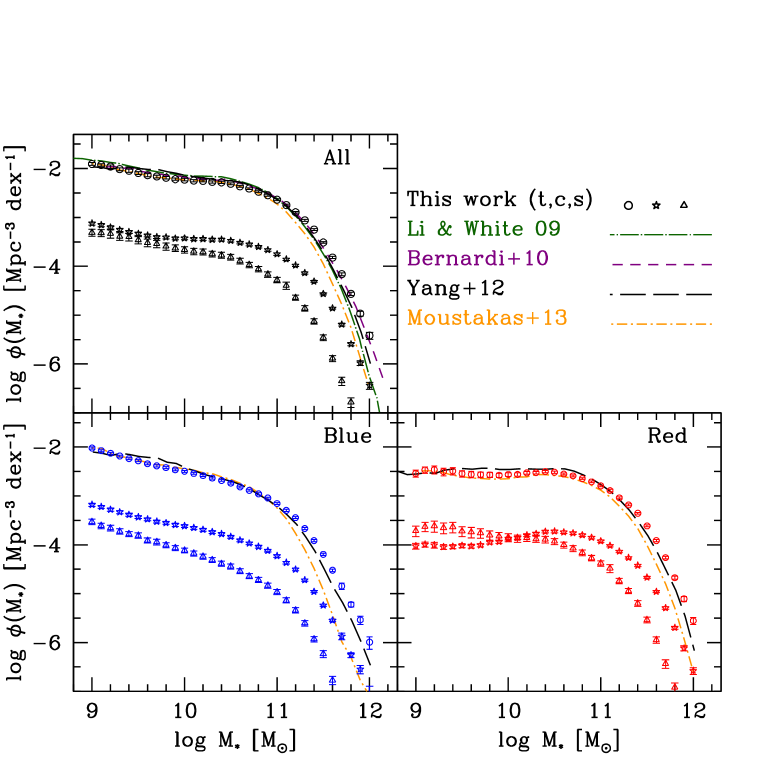
Figure 2.— Upper panel: The GSMF for all galaxies from the MPA-JHU NYU-VAGC/SDSS DR7 sample obtained and used in this paper (empty circles with error bars) compared with some GSMFs reported recently in the literature. Open stars and triangles with error bars show respectively the decomposition of the GSMF into central and satellite galaxies computed by using the Y12 galaxy group catalog. The data were shifted down by 1 dex in order to avoid overplotting. Lower panels: Corresponding blue and red GSMFs from the MPA-JHU NYU-VAGC/SDSS DR7 galaxies, as well as their decompositions into centrals and satellite galaxies. The orange dot-dashed line is for the active/passive GSMF decomposition in (Moustakas et al., 2013).

Table 1Fit parameters to the SDSS DR7 GSMFs

GSMF	$\log(\phi_{1}^{*})$	$\alpha_{1}$	$\log(\mathcal{M}^{*}_{1})$	$\log(\phi_{2}^{*})$	$\alpha_{2}$	$\beta$	$\log(\mathcal{M}^{*}_{2})$
(MPA-JHU $M_{*}$’s)	[Mpc-3 dex-1]		[M⊙]	[Mpc-3 dex-1]			[M⊙]
All $\ldots\ldots$	$-2.46\pm 0.30$	$-1.32\pm 0.22$	$9.55\pm 0.32$	$-2.24\pm 0.03$	$-0.64\pm 0.15$	$0.65\pm 0.04$	$10.49\pm 0.17$
Blue $\ldots\ldots$	$-3.07\pm 0.13$	$-1.58\pm 0.08$	$10.17\pm 0.13$	$-2.69\pm 0.07$	$-0.23\pm 0.20$	$0.51\pm 0.04$	$9.82\pm 0.19$
Red $\ldots\ldots$	–	–	–	$-2.60\pm 0.02$	$-0.79\pm 0.02$	$0.80\pm 0.02$	$10.83\pm 0.03$
(Corrected $M_{*}$’s; see §§5.4.2)
All $\ldots\ldots$	$-3.82\pm 0.20$	$-1.60\pm 0.06$	$11.64\pm 0.06$	$-2.44\pm 0.05$	$-0.15\pm 0.12$	$0.58\pm 0.06$	$10.14\pm 0.20$

As mentioned above, to constrain the model parameters we use the observed total blue and red GSMFs and the projected 2PCFs of blue and red galaxies at various stellar masses. In addition, we use the decomposition of the GSMFs into central and satellites computed from the Y12 galaxy group catalog.

3.1. Galaxy stellar mass functions

We construct the GSMFs from the New York Value Added Galaxy Catalogue, NYU-VAGC, based on the SDSS DR7. We use the sample selection as given in the halo-mass based group catalog of Y12. This galaxy group catalog represents an updated version of Yang et al. (2007). Therefore, our galaxy sample has the same cuts and depurations as in this catalog, for further details with respect to the group catalog see Yang et al. (2007). The total number of galaxies used for constructing the GSMF is 639,359. The Y12 catalog uses colors and magnitudes based on the standard SDSS Petrosian radius. Following Blanton et al. (2003) and Yang, Mo & van den Bosch (2009a), we use the evolution correction at $z=0.1$ given by $E(z)=1.6(z-0.1)$. For the K-correction, we use an analytical model as described in the Appendix. In this model, the K-correction term depends on both redshift and color, $g-r$, that is, $K=K(z,g-r)$. K-corrections and absolute magnitudes at $z=0.1$ computed within this scheme are accurately recovered with typical percentage errors less than $\sim 10\%$ and $\sim 1\%$ on average, respectively.

For the stellar masses, we use those reported in the MPA-JHU DR7 data base. These masses were calculated from photometry-spectral energy distribution fittings assuming a Chabrier (2003) IMF; for details, see Kauffmann et al. (2003). We found that in our sample approximately $\approx 9\%$ of the galaxies lack of stellar mass measurements. Since this fraction is not negligible, we decided to calculate the stellar masses for these galaxies by using the color-dependent mass-to-light ratio given by Bell et al. (2003). For this subsample of galaxies we applied a correction of $-0.1$ dex in order to be consistent with the Chabrier (2003) IMF adopted in this paper. Also, we checked that these galaxies are not particularly biased in mass or color. The masses of these galaxies were not determined likely due to issues in their spectra and/or the stellar populations synthesis fits.

Following Moustakas et al. (2013), for the calculation of the GSMF we adopt a flat stellar mass completeness limit of $\mbox{$M_{*}$}=10^{9}\mbox{M${}_{\odot}$}$. As noted by these authors, this limit is above the surface brightness and stellar mass-to-light ratio completeness limits of the SDSS, see Blanton et al. (2005); Baldry, Glazebrook & Driver (2008). The GSMF in here is estimated as

$$\phi_{g}(\mbox{$M_{*}$})=\frac{1}{\Delta\log\mbox{$M_{*}$}}\sum_{i=1}^{N}\frac{\omega_{i}}{V_{{\rm max},i}},$$ (30)

where $\omega_{i}$ is the correction wieight completeness factor in the NYU-VAGC and for each galaxy, $V_{\rm max,i}$ is given by

$$V_{{\rm max},i}=\int_{\Omega}\int_{z_{l}}^{z_{u}}\frac{d^{2}V_{c}}{dzd\Omega}dzd\Omega.$$ (31)

Here, $z_{l}=0.01$ and $z_{u}={\rm min}(z_{{\rm max},i},0.2)$, $\Omega$ is the solid angle of the SDSS DR7 and $V_{c}$ is the comoving volume (Hogg, 1999). The maximum redshift at which each galaxy can be observed, $z_{{\rm max},i}$, is computed by solving iteratively the distance modulus equation, i.e.,

$$m_{{\rm lim},r}-M_{r,i}^{0.1}=5\log D_{L}(z_{{\rm max},i})-25-K(z_{{\rm max},i})+E(z_{{\rm max},i}),$$ (32)

and each observed galaxy should satisfy the apparent magnitude of the Y12 group catalog, $m_{{\rm lim},r}=17.72$. The term $D_{L}(z)$ is the distance modulus (Hogg, 1999).

For each stellar mass bin, errors are computed using the jackknife technique. We do so by dividing Y12 galaxy group sample into 200 subsamples of approximately equal size and each time calculating $\phi_{g,i}(\mbox{$M_{*}$})$. Then, errors are estimated as

$$\sigma_{\phi}=\left[\frac{N-1}{N}\sum_{i=1}^{N}(\phi_{g,i}-\langle\phi_{g}\rangle)^{2}\right]^{1/2},$$ (33)

where $N=200$, $\phi_{g,i}$ is the GSMF of the sample $i$, and $\langle\phi_{g}\rangle$ is the average over the ensemble.

We divide our galaxy sample into two wide groups, blue and red galaxies. This division roughly correspond to late-type/star-forming and early-type/passive galaxies, respectively. Note that for this division, we are using K-corrected colors to $z=0.1$, ${}^{0.1}(g-r)$. Red/blue galaxies are defined based on the Li et al. (2006) color-magnitude criteria. These authors separated galaxies into blue and red by using a bi-Gaussian fitting model to the color distribution in many absolute magnitude bins; see Li et al. (2006) for details. Because of dust extinction, blue star-forming and highly inclined galaxies could be classified as a red passive galaxies (e.g., Maller et al., 2009). In §§5.1 we discuss the impact of this possible contamination in our color division.

Finally, we also divide our galaxy sample into central and satellite galaxies according to the galaxy groups identified in the latest version of the Yang et al. (2007) group catalog. In this paper, we define central galaxies as the most massive galaxies within their group.

3.1.1 Total galaxy stellar mass functions

Figure 2 shows the resulting SDSS MPA-JHU DR7 GSMFs for all, blue and red galaxies estimated as described above (empty circles with error bars). For comparison, in the upper left panel of the same figure we reproduce local estimations of the total GSMFs based on SDSS reported in Li & White (2009); Bernardi et al. (2010); Yang et al. (2012) and Moustakas et al. (2013). In the bottom left and right panels we reproduce the Y12 GSMFs corresponding to blue and red galaxies, as well as the Moustakas et al. (2013) GSMFs corresponding to active and passive galaxies. Note that the GSMFs separated into blue and red components according to the Li et al. (2006) color-magnitude criteria are similar to those of active and passive GSMFs (from Moustakas et al., 2013) for $\mbox{$M_{*}$}\lower 2.15277pt\hbox{$\;\buildrel<\over{\sim}\;$}10^{11}\mbox{M${}_{\odot}$}$.

In general, our NYU-VAGC/SDSS MPA-JHU DR7 GSMFs for all, blue and red galaxies are consistent with previous estimates, except at the high-mass end, which has a shallower fall than most of previous ones, but in good agreement with the total GSMF from Bernardi et al. (2010). In fact, the function could be even shallower if one takes into account accurate photometric profile fits when calculating total luminosities or $M_{*}$ (Bernardi et al., 2013). In Section 5.4.2, we apply corrections to our galaxy stellar masses in order to take into account this effect.

As reported by previous authors, we find that a single Schechter function is not consistent with the total GSMF (see e.g., Baldry, Glazebrook & Driver, 2008; Li & White, 2009; Drory et al., 2009; Pozzetti et al., 2010; Baldry et al., 2012; Moustakas et al., 2013; Bernardi et al., 2013; Tomczak et al., 2014). Besides, the high-mass end of our GSMF is shallower than an exponential decay. For completeness, we present the best fits to our GSMFs. Following Bernardi et al. (2010), we fit our GSMFs by using a function that is composed of a single Schechter plus a Schechter function with a sub-exponential decay at the high-mass end,

$$\phi_{g}(X)dX=\phi_{1}^{*}X_{1}^{\alpha_{1}}e^{-X_{1}}dX_{1}+\phi_{2}^{*}X_{2}^{\alpha_{2}}e^{-X_{2}^{\beta}}dX_{2},$$ (34)

where $X_{i}=\mbox{$M_{*}$}/\mathcal{M}^{*}_{i}$ with $i=1,2$. The corresponding best-fit parameters are reported in Table 1. For blue galaxies we also employed Eq. (34), while for red galaxies we find that a single Schechter function with a sub-exponential decay gives a good fit to the data. The parameters of these fits are also given in Table 1.

3.1.2 Central and Satellite galaxy stellar mass functions

Figure 2 shows our measurements of the central (stars) and satellite (triangles) GSMFs for all, blue and red galaxies. In order to avoid overplotting, we have shifted down these GSMFs by $1$ dex. The Y12 galaxy group catalog has been used to define central and satellite galaxies; we assume that a central is the most massive galaxy in its group.

The blue satellite GSMF lies significantly below the blue central GSMF at all masses. In contrast, for red galaxies, at masses below $\mbox{$M_{*}$}\sim 10^{10}\mbox{M${}_{\odot}$}$, the red GSMF is dominated by satellite galaxies, roughly by a factor of $\sim 2.5$ above centrals. For larger masses, the trend inverts and the red GSMF is already dominated by red centrals. When comparing blue and red central GSMFs, for $\mbox{$M_{*}$}\lower 2.15277pt\hbox{$\;\buildrel<\over{\sim}\;$}10^{10.3}$ M_⊙, the abundances of red centrals are lower than those of blue centrals. For $\mbox{$M_{*}$}\gtrsim 10^{10.3}$ M_⊙, red centrals become the dominant population. In the case of satellite galaxies, the abundances of blue satellites are lower than those of red satellites for practically all masses.

Finally, note that for constraining our model parameters, we are not including the full covariance matrix of the different GSMFs derived in this work.

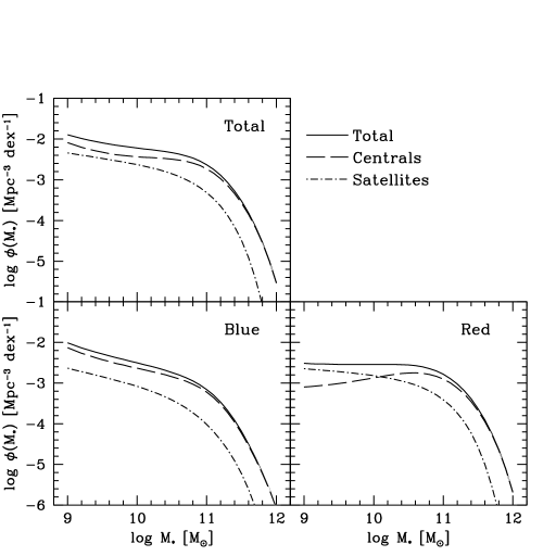
Figure 3.— Model GSMFs. Each panel shows the fitted total, blue and red GSMFs (solid lines). The long-dashed and dot-dashed lines show the decomposition of the GSMFs into central and satellite galaxies, respectively.

3.2. Correlation functions

For the correlation functions, we use the Li et al. (2006) measurements of the projected 2PCF, $\omega_{p}(r)$, in five different stellar mass bins and for all, blue, and red galaxies. This measurements were done based on a sample of $\sim 2\times 10^{5}$ galaxies from the SDSS DR2. Note that (1) the color-magnitude criterion to separate galaxies into blue and red by Li et al. (2006) is the same one we have used for constructing the blue and red GSMFs, and (2) in the calculation of our GSMFs, we use the same stellar mass inferences as in Li et al. (2006).

In our analysis, we are using only the diagonal of the covariance matrix given in Li et al. (2006). Unfortunately, the full covariance matrix is not available (Cheng Li, private communication).

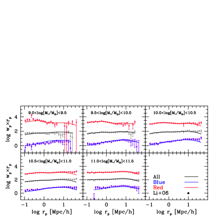
Figure 4.— Projected 2PCFs for all, blue and red galaxies in five different stellar mass bins. Best fit models are shown with solid lines, while measurements based on the SDSS DR2 from Li et al. (2006) are shown with the filled circles with error bars. In order to get a better visual comparison between our fits and observations we plot $\omega_{p}\times r_{p}$ instead $\omega_{p}$.

4. Results

To sample the best fit parameters in our model we run a set of $3\times 10^{5}$ MCMC models. We obtained the following best fitting parameter:

• Mean SHMR of blue central galaxies (Eqs. 17-18):

  $$\begin{array}[]{c}\log\epsilon_{b}=-1.593\pm 0.042\\ \log M_{1,b}=11.581\pm 0.034\\ \alpha_{b}=1.500\pm 0.148\\ \delta_{b}=4.293\pm 0.271\\ \gamma_{b}=0.396\pm 0.035\\ \end{array}$$ (35)

  
  

• Mean SHMR of red central galaxies (Eqs. 17-18):

  $$\begin{array}[]{c}\log\epsilon_{r}=-2.143\pm 0.086\\ \log M_{1,r}=11.367\pm 0.100\\ \alpha_{r}=2.858\pm 0.479\\ \delta_{r}=6.026\pm 0.544\\ \gamma_{r}=0.303\pm 0.023\\ \end{array}$$ (36)

  
  

• Scatters of the blue/red SHMRs (Eqs. 15,16):

  $$\begin{array}[]{c}\sigma_{b}=0.118\pm 0.020\\ \sigma_{r}=0.136\pm 0.010\\ \end{array}$$ (37)

  
  

• Fraction of blue centrals as a function of $M_{\rm h}$ (Eq. (21):

  $$\begin{array}[]{c}\beta=0.688\pm 0.065\\ b=1.032\pm 0.014\\ \end{array}$$ (38)

• Occupation of satellite galaxies (Eqs. 22-26):

  $$\begin{array}[]{c}\alpha_{s,b}=-1.251\pm 0.024\\ \phi_{0,b}=-1.324\pm 0.039\\ \phi_{1,b}=0.540\pm 0.025\\ c_{0}=10.863\pm 0.037\\ c_{b}=0.192\pm 0.020\\ c_{r}=0.087\pm 0.016\\ \alpha_{s,r}=-1.096\pm 0.014\\ \phi_{0,r}=-1.363\pm 0.024\\ \phi_{1,r}=1.051\pm 0.010\\ \end{array}$$ (39)

For our best fitting model we find that the total $\chi^{2}=1139$ from a number of $N_{d}=666$ observational data points. Since our model consist of $N_{p}=23$ free parameters the resulting reduced $\chi^{2}$ is $\chi^{2}/{\rm d.o.f.}=1.77$. Figure 16 in Appendix C shows the posterior probability distributions of the model parameters. This plot gives a visual information of the covariances between the model parameters. In almost all the cases, the parameters do not correlate between each other.

4.1. GSMFs and correlation functions

In each panel of Fig. 3 we plot the best-fit model GSMFs for all, blue and red galaxies (solid lines). In the same panels, we show the decomposition of the GSMFs into central (long-dashed lines) and satellites (dot-short-dashed lines) corresponding to all, blue and red galaxies. In general, our model fits describe well the observed GSMFs, decomposed into central and satellites (compare Fig. 3 with Fig. 2).

Figure 4 shows the observed projected 2PCFs reported in Li et al. (2006, filled circles with error bars) and the best model fits (solid lines). The projected 2PCFs are for all, blue, and red galaxies (black, blue and red colors, respectively) in five different stellar mass bins. In order to get a better visual comparisons of our fits to observations, we plot $\omega_{p}\times r_{p}$ (instead of $\omega_{p}$) as a function of $r_{p}$. For clarity, our fits and the data points for blue and red galaxies have been shifted by +1 dex and -1 dex, respectively. In general, our fits describe well the observations for all mass bins and in almost all separations. We note, however, that at large separations our fits tend to lie below observations in the stellar mass bins $10<\log(\mbox{$M_{*}$}/\mbox{M${}_{\odot}$})<10.5$ and $10.5<\log(\mbox{$M_{*}$}/\mbox{M${}_{\odot}$})<11$. It is known that at large separations the correlation functions are affected by cosmic variance in volume-limited samples. This effect in the SDSS galaxies has been investigated in detail by Zehavi et al. (2005) and Zehavi et al. (2011), where the authors find that the most significant cosmic variance effect appears due to the presence of a supercluster at $z\sim 0.08$, the Sloan Great Wall (Gott et al., 2005). These authors conclude that the inclusion of this supercluster in the calculation of the correlation functions causes an anomalous high amplitude of galaxy clustering at large separations in samples with $-21<M_{r,0.1}<-20$. This magnitude bin roughly corresponds namely to a stellar mass bin $10<\log(\mbox{$M_{*}$}/\mbox{M${}_{\odot}$})<11$. Thus, the observational values of $\omega_{p}$ at large radii in this mass bin could be overestimated.

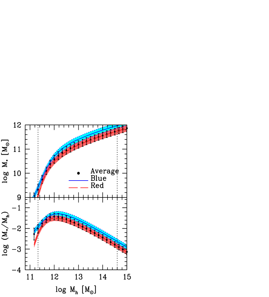
Figure 5.— Upper panel: Inferred SHMRs of blue and red central galaxies (blue and solid lines, respectively) and the density-averaged SHMR (dots). The shaded areas and error bars are their corresponding constrained scatters ($\sigma_{j}$), which can be considered as upper limits to the intrinsic scatters. Bottom panel: The $M_{*}$-to-$M_{\rm h}$ ratio as a function of $M_{\rm h}$ for the same cases plotted in the top panel. Note that the density-averaged SHMR approaches the red SHMR at large masses, while at lower masses is in between the blue and red SHMRs. The dotted vertical lines indicate the lower and upper limits in halo mass at which our average SHMR can be robustly constrained.

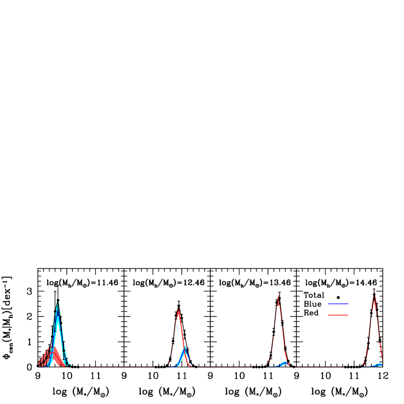
Figure 6.— Inferred blue and red central conditional stellar mass distributions at different halo masses (red and blue lines). The shaded areas are the $1\sigma$ error due to the uncertainties in the model parameters. The dotted points with error bars show the total central conditional distributions. Note the there is a bimodality at low halo masses, while at large masses the total distribution is dominated by red central galaxies.

In order to quantify the effect of cosmic variance in our fits, we have excluded separations larger than $r_{p}>10h^{-1}$ Mpc in the projected 2PCFs in the bins that encompass masses in the range $10<\log(\mbox{$M_{*}$}/\mbox{M${}_{\odot}$})<11$ and recalculated the $\chi^{2}/$d.o.f by using our best fit parameters. The exclusion of these separations leads to a substantial decrease in the reduced $\chi^{2}$, $\chi^{2}/$d.o.f.$=1.47$. This implies that cosmic variance effects could affect our fits. To test this, we have recalculated our model parameters using this modified data set regarding the 2PCFs. As a result, we found that the values of all the model parameters remain similar to those obtained previously, particularly those related to the SHMRs. The insensitivity of HOD model parameters to the data at large separations has been reported previously (see e.g., Zehavi et al., 2011). The reason is that for a fixed cosmology, the HOD parameters have less freedom to adjust the large-scale correlation relative to the (more) robust inferences at small separations, $r_{p}<2h^{-1}$Mpc. Therefore, we conclude that our model fit parameters are robust against uncertainties due to cosmic variance in the 2PCFs at large separations.

On the other hand, in the stellar mass bin $9<\log(\mbox{$M_{*}$}/\mbox{M${}_{\odot}$})<9.5$ we note that our fits tend to be slightly below observations at small separations. It is not clear the reasons behind this difference but we have quantified the impact of it in our goodness-of-fit. Similarly done for large separations, we have recalculated the $\chi^{2}/$d.o.f. but this time excluding the information of the correlation functions at this mass bin. The resulting $\chi^{2}/$d.o.f. is 1.71. This means that the correlation function from this stellar mass bin does not add substantial information to constrain our model parameters. Note, however, that in order to obtain robust inferences of our model parameters, we have also included the information of the central and satellite GSMFs.

4.2. Stellar-to-Halo Mass Relations

The derivation of the SHMRs and their scatters for local blue and red central galaxies is the main goal of this paper. These mass relations and the corresponding $M_{*}$-to-$M_{\rm h}$ ratios vs. $M_{\rm h}$, as constrained by means of our model, are shown in the upper and lower panels of Fig. 5. Blue solid and red long-dashed lines show the mean relations of blue and red centrals, respectively. Shaded areas show the standard deviations of the (lognormal-distributed) scatter (see Section 2.3.1 and Eq. 15). Recall that this scatter is composed by an intrinsic component and by a measurement error component (Eq. 16). This scatter should be considered as an upper limit of the intrinsic component. In Section 4.2.1, we estimate values for the intrinsic scatters once we introduce conservative estimations for measurement error components. Black dots with error bars represent the average central relations, calculated as in Eq. (19), and its corresponding scatter (standard deviation, calculated using Eq. 20). Recall that Eq. (19) is a density-weighted average, so the mean SHMR for all central galaxies is located in between the SHMRs of blue and red centrals. However, at high masses the average SHMR is practically equal to the one of red galaxies. This is because almost all massive halos host red central galaxies, see below. The dotted vertical line indicates the lower limit in halo mass at which our average SHMR has been robustly constrained. Note that we did not assume any functional form both for the shape and for the scatter of the average SHMR. Instead, they are a direct prediction and the result of constraining separately the SHMRs of blue and red central galaxies.

Our results point out that the SHMRs of blue and red centrals are different. In other words, the SHMR of central galaxies is segregated by color. For a given $M_{\rm h}$, the $M_{*}$ or $M_{*}$-to-$M_{\rm h}$ ratio of blue galaxies is always larger than the one of red centrals. The minimum difference is of 0.16 dex at $M_{\rm h,min}=5\times 10^{11}$ M_⊙, close to the mass where the halos contain the same fraction of blue and red centrals (see below, §§4.3). The difference increases up to $\approx 0.24$ dex at $\mbox{$M_{\rm h}$}=5\times 10^{12}$ M_⊙ and for larger masses it remains roughly constant. For masses $<M_{\rm h,min}$, the difference strongly increases. At any mass, the differences are larger than the $1\sigma$ scatter of the relations, $\sigma_{b}$ and $\sigma_{r}$, respectively (see also §§4.2.1 below). This can be also appreciated in Fig. 6, where we plot the conditional stellar mass distributions of blue and red central galaxies for four different halo masses, blue and red lines, respectively. The shaded areas show the $1\sigma$ confidence intervals around these relations. The dots with error bars show the same but for all central galaxies. The distributions of blue and red centrals, which are related to the scatters around the corresponding SHMRs, are different. Besides, as it will be shown in the next subsection and in Fig. 7, the scatters around the constrained blue and red SHMRs compared to the $1\sigma$ confidence intervals obtained from our MCMC run are smaller than the corresponding scatters. Thus, the differences in the values of the mean SHMRs of blue and red centrals are significant also at the level of error analysis.

Figure 6 shows that for $\mbox{$M_{\rm h}$}\lower 2.15277pt\hbox{$\;\buildrel<\over{\sim}\;$}3\times 10^{11}$ M_⊙, the galaxy population of centrals is dominated by blue galaxies over the red ones, while at $\mbox{$M_{\rm h}$}\sim 3\times 10^{12}$ M_⊙, red galaxies are already the dominant population but there is yet a non-negligible fraction of blue galaxies. Instead, at $\mbox{$M_{\rm h}$}\sim 3\times 10^{13}$ M_⊙, practically all central galaxies are red. It is at masses $10^{11.5}\mbox{M${}_{\odot}$}\lower 2.15277pt\hbox{$\;\buildrel<\over{\sim}\;$}\mbox{$M_{\rm h}$}\lower 2.15277pt\hbox{$\;\buildrel<\over{\sim}\;$}10^{12.5}\mbox{M${}_{\odot}$}$ that the SHMR of central galaxies has a clear bimodal distribution. At larger and lower masses, the average SHMR for all central galaxies is practically given by the SHMR of red and blue centrals, respectively (Fig. 5).

4.2.1 The scatter of the SHMRs

In our model, we have assumed that the stellar mass distribution of both blue and red central galaxies are lognormal. Additionally, we assumed that the widths (scatters) of these distributions are free parameters in our model. Recall, that these scatters were assumed independent of $M_{\rm h}$ (Eq. 15). The values constrained for these scatters are $\sigma_{b}=0.118\pm 0.020$ dex and $\sigma_{r}=0.136\pm 0.010$ dex, respectively (solid blue and short-dashed red lines surrounded by shaded areas in Fig. 5). In other words, the scatter around the SHMRs of red and blue central galaxies is higher for the former than for the latter, though the error bars overlap slightly. This implies that the SHMR of blue central galaxies is tighter than the one of red centrals.

The scatter around the density-averaged (blue + red) SHMR, $\sigma_{A}$, is plotted in Fig. 7 (black long-dashed line) along with $1\sigma$ confidence interval (gray shaded area). Similarly to Fig. 5, the dotted vertical line indicates the lower limit in halo mass at which the scatter $\sigma_{A}$ has been robustly constrained. For $\mbox{$M_{\rm h}$}\sim 10^{11.3}$ to $\sim 10^{15}$ M_⊙, $\sigma_{A}$ changes from $\sim 0.20$ dex to $\sim 0.14$ dex. Note that $\sigma_{A}$ is constant for masses above $\mbox{$M_{\rm h}$}\sim 10^{13}$ M_⊙. The dependence of $\sigma_{A}$ on $M_{\rm h}$ naturally arises according to Eq. (8). Because the majority of high mass halos, $M_{\rm h}$$\;\buildrel>\over{\sim}\;$$10^{13.5}$ M_⊙, host red central galaxies (see Fig. 6; see also Fig. 8 below) then $\sigma_{A}\sim\sigma_{r}\approx 0.14$ dex. In contrast, the increasing of $\sigma_{A}$ with decreasing $M_{\rm h}$ is the result of the color bimodality in the average SHMR for masses below $\mbox{$M_{\rm h}$}\lower 2.15277pt\hbox{$\;\buildrel<\over{\sim}\;$}10^{12.5}$ M_⊙ (see Fig. 6).

As mentioned in §§2.3.1, the scatters $\sigma_{j}$ reported above consist of an intrinsic component, $\sigma_{j}^{\rm i}$, and of measurement errors component, $\sigma_{j}^{\rm e}$, see Eq. (16). Following the results by Behroozi, Conroy & Wechsler (2010) and Leauthaud et al. (2012), we assume that the dominant source of measurement error comes from individual stellar mass estimates. For the data employed in our analysis, we used stellar masses from an update of Kauffmann et al. (2003). In that paper, the authors found that the 95 per cent confidence interval from their stellar mass estimates is typically a factor of $\sim 2$ in mass. As noted by the authors, in a Gaussian distribution this corresponds to four times the standard error, resulting in a standard deviation of $\sim 0.075$ dex. This is consistent with the standard deviation reported in Conroy, Gunn & White (2009) for local luminous red galaxies. Measurement errors might be different between red and blue galaxies, for example Kauffmann et al. (2003) found that these errors are somewhat smaller for older galaxies with ${\rm D}_{n}(4000)>1.8$ than for younger galaxies with ${\rm D}_{n}(4000)<1.8$. Unfortunately, the authors do not provide values for their confidence intervals.

We assume a conservative value of $\sigma_{j}^{\rm e}=0.07$ dex for both blue and red central galaxies. We estimate the intrinsic scatters of blue and red central galaxies by deconvolving from measurement errors using the $3\times 10^{5}$ MCMC models generated for fitting the data. We estimate conservatives values of $\sigma_{b}^{\rm i}=0.094\pm 0.024$ and $\sigma_{r}^{\rm i}=0.116\pm 0.012$ for blue and red centrals, respectively.

Finally, in Fig. 7, we also plot the magnitude of the $1\sigma$ confidence intervals around the mean SHMRs for blue, red and all central galaxies (solid blue, short-dashed red, and long-dashed black lines without shaded areas, respectively). These confidence intervals were obtained from the $3\times 10^{5}$ MCMC models generated to sample the best fit parameters in our model. The confidence intervals take into account the error bars from our set of observational constraints. Note that we are not taking into account any source of systematical uncertainty, which are usually dominated by systematical uncertainties in stellar mass inferences and they may be up to $0.25$ dex (Behroozi, Conroy & Wechsler, 2010). The confidence intervals around the mean SHMR of all central galaxies (black long-dashed line) are much smaller than the scatter $\sigma_{A}$ (black long-dashed line surrounded by a gray area). Similarly, the confidence intervals around the mean SHMRs of blue and red central galaxies are much lower than their scatters $\sigma_{j}$, excepting at low and high masses for red and blue galaxies, respectively. At these masses, the $1\sigma$ confidence intervals around the mean SHMRs increase due to the scarce data and large observational error bars in these limits.

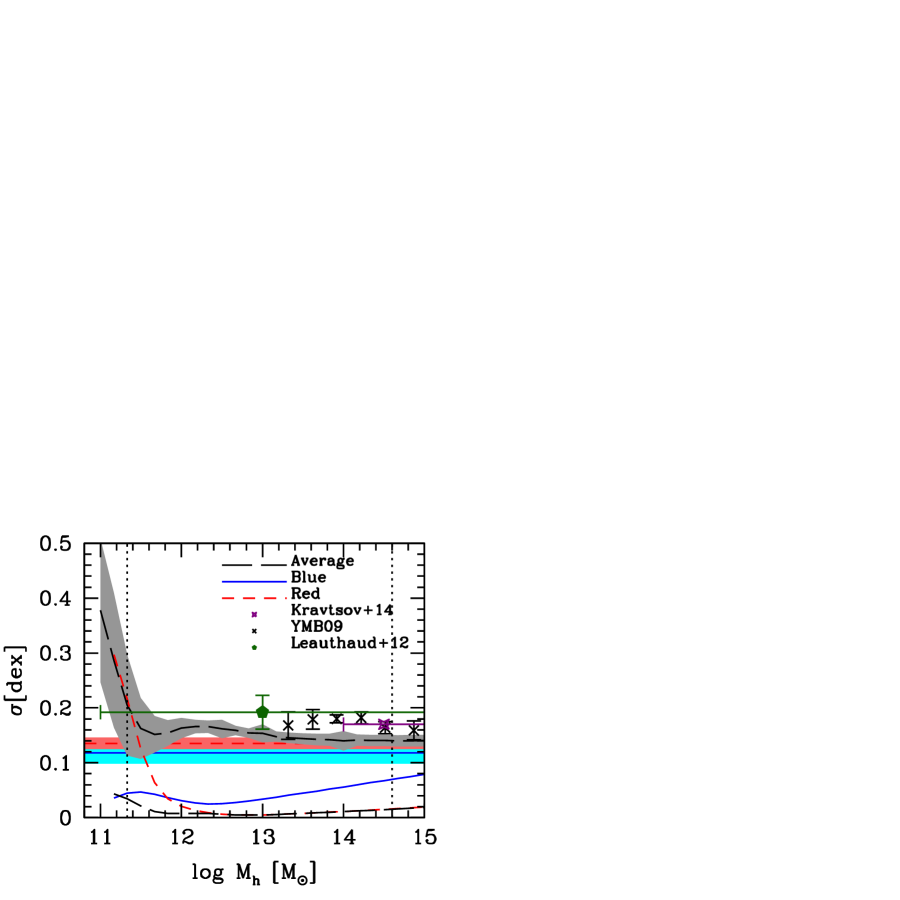
Figure 7.— Different type of scatters around the SHMRs. Blue solid, red short-dashed and black long-dashed lines are the constrained scatters, $\sigma_{b}$, $\sigma_{r}$ and $\sigma_{A}$, which can be considered as upper limits to the respective intrinsic scatters (see text); the shaded areas are the corresponding $1\sigma$ confidence intervals. Note that $\sigma_{A}$ changes with mass, while $\sigma_{b}$ and $\sigma_{r}$ were assumed to be constant. The bottom blue solid, red short-dashed and black long-dashed lines are the magnitude of the $1\sigma$ confidence intervals from $3\times 10^{5}$ MCMC trials for the blue, red and average SHMRs, respectively. Additionally, we have plotted the scatter constrained by Yang, Mo & van den Bosch (2009a, skeletal symbols), Leauthaud et al. (2012, filled pentagon), and Kravtsov, Vikhlinin & Meshscheryakov (2014, open star). The dotted vertical lines indicates the lower and upper limits in halo mass at which the intrinsic scatter $\sigma_{A}$ can be robustly constrained.

Figure 8.— Upper panel: Inferred fraction of halos hosting central blue and red galaxies as a function of $M_{\rm h}$, blue and red solid lines, respectively. The blue and red shaded areas correspond to the $1\sigma$ confidence intervals. Most of the symbols with error bars are observational inferences using galaxy-galaxy weak lensing, see text. Long dashed line show the best fitting model from Tinker et al. (2013) based on the combined analysis of galaxy weak-lensing and clustering from COSMOS field at $z=0.36$. Skeletal symbols show the fraction of blue centrals from Skibba & Sheth (2009) model. Bottom panel: The same fraction of central blue galaxies as in the upper panel but as a function of $M_{*}$. Solid circles with error bars are results from the Y12 galaxy group catalog.

4.3. The fraction of halos hosting blue/red central galaxies

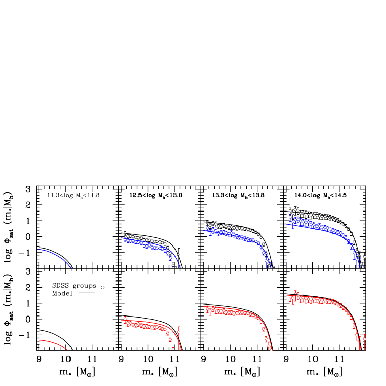
Figure 9.— Upper Panels: Satellite CSMFs of all and blue galaxies for four different halo mass bins (indicated inside the panels). Solid lines are for the model predictions and open circles with error bars are from Y12 group catalog; black and blue colors are for all and only blue satellites, respectively. Lower Panels: As in in the upper panel but for red satellite galaxies only. For comparison black solid lines reproduce our best fitting model for the satellite CSMFs of all galaxies.

We have parametrized the fraction of halos hosting blue/red (approximately active/quenched) central galaxies by using a general observationally-motivated dependence, see §§2.3.1. In Fig. 8, we show the constrained blue fraction as a function of $M_{\rm h}$, $\mbox{$f_{\rm blue}$}(\mbox{$M_{\rm h}$})$. Recall that $f_{\rm blue}$ is the complement of $f_{\rm red}$, $\mbox{$f_{\rm blue}$}(\mbox{$M_{\rm h}$})=1-\mbox{$f_{\rm red}$}(\mbox{$M_{\rm h}$})$. The fraction of blue centrals decreases with $M_{\rm h}$ roughly a factor of $\sim 4.4$ from $\mbox{$M_{\rm h}$}\approx 10^{11}$ to $\approx 10^{12.5}$ M_⊙.

Our results show that $b\approx 1$ in Eq. (21). This means that the dependence of $f_{\rm red}$ on $M_{\rm h}$ is actually close to the one suggested in Woo et al. (2013) based on the empirical inferences of Peng et al. (2012). In this case, the characteristic halo mass where the fraction of halos hosting blue and red centrals is the same, i.e., $f_{\rm blue}=f_{\rm red}=0.5$ is given by: $\mbox{$M_{\rm h}$}=6.88\pm 0.65\times 10^{11}$M_⊙. For Milky-Way sized halos, $\mbox{$M_{\rm h}$}\sim 10^{12}\mbox{M${}_{\odot}$}$, the blue (red) fraction is $\sim 1/3$ ($\sim 2/3$).

In Fig. 8, we reproduce also some direct observational inferences obtained by stacking weak-lensing data: Mandelbaum et al. (2006, open circles), van Uitert et al. (2011, open squares) and Velander et al. (2014, open triangles). In general, our result is in reasonable agreement with these direct inferences. We also compared our resulting fraction with the analysis of satellite kinematics performed in More et al. (2011, gray shaded area). The shift observed with respect to our results is possible related to the fact that halo masses measured from satellite kinematics are usually higher than other methods, see Section 5.4. We also compare our results with those of Tinker et al. (long dashed-line 2013). Note, however, that the blue fraction from Tinker et al. (2013) is higher that for local galaxies. One possibility is that the fraction of halos hosting blue centrals is expected to be higher than for $z\sim 0$. Another reason is that due to sample variance in the COSMOS field at $z\sim 0.36$, it may not possible to obtain a direct comparison with our results (Jeremy Tinker, private communication). We also include a comparison with results from Skibba & Sheth (2009). Although at low masses their results are consistent with our blue fraction, at the high mass end there is a discrepancy. This is possible related to the fact the the Skibba & Sheth (2009) model assumes that color depends only weakly on mass. Finally, it is important to note, that the way the two galaxy populations are separated in all the studies mentioned above, may vary with most of the authors (based on colors, specific star formation rate, type, etc.). This introduces differences in the fractions plotted in Fig. 8. In spite of that, the overall result is consistent among most of the studies.

For completeness, the lower panel of Fig. 8 shows our model fitting (solid line with a shaded area) to the empirical fraction of blue central galaxies as a function of $M_{*}$, i.e. the ratio of blue-to-all central GSMFs from the Y12 galaxy group catalog (solid circles with error bars).

4.4. The blue/red satellite CSMFs

Figure 9 shows the predicted CSMFs for all, blue and red satellites (Eqs. 22–26). For comparison, the circles with error bars in all the panels show the same but for the Y12 galaxy group catalog (we use only those groups that are complete according to the completeness limits discussed in Section 2.2 of Yang, Mo & van den Bosch (2009a) for both halo and stellar masses). We have corrected their halo masses to match our virial halo mass definition, see Eq. (B1) in Appendix B. Error bars were estimated by using the jackknife method described in Section 3 with $N=200$. We have also weighted each galaxy by a factor of $V/V_{\rm max}$. In general, both the amplitude and the shape of the predicted CSMFs agree with those from the Y12 group catalog. In more detail, for massive halos, the predicted CSMFs for blue satellites are shallower in the low-mass end ($\mbox{$M_{*}$}\approx 10^{10}\mbox{M${}_{\odot}$}$) than the inferred ones from the group catalogs but within the error bars. One possible reason is the relative poor constraints from the lowest mass bin from $\omega_{p}$, see the discussion in Section 4.1.

5. Discussion

5.1. Robustness of the results

The segregation in color found in the SHMR of central galaxies in Section 4 is a relevant result. How robust is it? We have carried out several experiments in order to explore this question. For example, we have explored what happens if we force the SHMR of blue and red centrals as well as their scatter to be identical. In this case, we find that the best fits to observations are poorer than those obtained in Section 4, with $\chi^{2}/$d.o.f.$=2.1$, which is $\sim 25\%$ larger than in that Section. We have also checked what fraction of our $3\times 10^{5}$ MCMC models have similar parameters in their parametrization for the blue and red SHMRs. First, note that most of the error bars in each model parameter is of the order of $\sim 10\%$ of the value of the parameter. When allowing this relative difference of $\sim 10\%$ between models we could not found any model. By allowing for relative differences in the parameters up to a 50%, only a $\approx 3\%$ of the MCMC models obey this condition. Therefore, in the search of the best fits, the cases of similar blue and red SHMRs are really rare.

In addition, we have found (as expected) that the key ingredient of the color segregation in the SHMR is the fraction of halos hosting red (blue) centrals as a function of $M_{\rm h}$. This fraction, according to our results, is essentially defined by the parameter, $M_{\rm h}^{\star}$ (see Eq. 21) and in less degree by the parameter $b$. Under the assumption that the SHMR of blue and red centrals are identical and keeping all the parameters for satellite galaxies as obtained in Section 4, excepting $M_{\rm h}^{\star}$, we find that the best fits that minimize $\chi^{2}$ is with $\mbox{$M_{\rm h}^{\star}$}\approx 9.7\times 10^{11}$ M_⊙, i.e., $\sim 1.4$ times larger than the one found in Section 4. The fits to observations in this cases are very poor, giving a total $\chi^{2}/$d.o.f$\approx 4.7$. This difference shows that the segregation in color is sensitive to the value of $M_{\rm h}^{\star}$. If now $M_{\rm h}^{\star}$ is fixed to larger values than $\sim 10^{12}$ M_⊙, and one allows for a difference between the SHMR of blue and red galaxies, then we obtain that the constrained SHMRs differ in an opposite way as found in Section 4 (obviously, the fits become even much poorer). On the other hand, as $M_{\rm h}^{\star}$ becomes smaller, the difference between the SHMRs in the direction of blue galaxies gets larger $M_{*}$ for a given $M_{\rm h}$ than red ones.

We also explored the case of generalizing the function Eq. (21) by allowing the mass term in the denominator to vary as $(\mbox{$M_{\rm h}^{\star}$}/\mbox{$M_{\rm h}$})^{a}$. We have found that the best fit is obtained when $a\approx 1$, that is, the proposed function Eq. (21) is robust. The resulting SHMRs in this case are very close to those obtained in Section 4, where $a=1$ is assumed. Along the same vein, if we modify partially our parametric approach, then the obtained SHMRs do not change significantly, though other predictions may already differ. For instance, this was the case when we modeled the satellite CSMFs through the SHAM between the theoretical subhalo mass function and the (predicted) satellite GSMF (case B in RAD13), instead of proposing parametric functions for the CSMFs.

In our model, we assumed $\sigma_{b}$ and $\sigma_{r}$ as free parameters. The resulting constrained values were $\sim 0.11$ and $\sim 0.14$, respectively. On the other hand, these parameters can be also obtained directly from the group galaxy catalogs, especially for massive halos Yang, Mo & van den Bosch (see e.g., 2009a), which are slightly different form our model constraints, see Section 5.3 below. To test the impact of this, we repeat our analysis but this time we fix $\sigma_{b}=\sigma_{r}=0.15$ dex. As we describe in Section 5.3, $\sigma_{b}\approx\sigma_{r}\approx 0.15$ dex as derived directly from the Yang et al. (2007) galaxy group catalog. In this case, we obtain a reduced $\chi^{2}$ similar to the one obtained in Section 4 (eq. 37), where we left $\sigma_{b}$ and $\sigma_{r}$ as free parameters. It should be said that the blue and red SHMRs obtained in the former case results slightly shallower at the high-mass end than those reported in Section 4. However, the relative separation between these two relations remains roughly the same, showing that our result that the SHMR segregates significantly by color is robust to changes in the $\sigma_{b}$ and $\sigma_{r}$ parameters.

Finally, we have explored the sensitivity of the blue/red central SHMRs to the observational constraints. In particular, in one experiment we renounced to use as constraints the central/satellite GSMF decompositions based on the Y12 group catalog, only the total blue/red GSMFs (and the 2PCFs) were used. Again, the constrained blue, red and average central SHMRs, remained almost the same. In this experiment, the central/satellite GSMFs are predicted; they are in reasonable agreement with those obtained with the Y12 group catalog, excepting the low-mass end of the blue satellite GSMF, which also implied a poor agreement with the Y12 CSMFs of blue satellites at low stellar masses in halos smaller than $\sim 10^{13}$ M_⊙.

5.1.1 On the blue/red separation criterion

In this paper, central galaxies were separated into blue and red galaxies by using the color-magnitude criterion of Li et al. (2006). While this separation is very rough, some of the results discussed in Section 4 could be sensitive to it. It is well known that there is not a perfect correspondence between blue/red galaxies and disk-/bulge-dominated or active/passive ones (c.f. Maller et al., 2009; Bundy et al., 2010; Woo et al., 2013). Late-type (blue) galaxies can appear in our separation as early-type (red) galaxies if they color is red due to dust extinction, specially when they are highly inclined and massive.

In order to evaluate the sensitivity of our results to dust extinction effects, we compare our fraction of blue (red) galaxies as a function of absolute magnitude in the $r$-band at $z=0.1$, ${}^{\rm 0.1}M_{r}$, with the one presented in Jin et al. (2014). These authors analyzed a subsample of the SDSS DR7 galaxies by selecting face-on galaxies only. By means of the $(u-r)_{\rm 0.1}$ color-magnitude diagram, they separate their sample into blue, red, and green galaxies, the latter are actually a small fraction ($<15\%$). The ${}^{\rm 0.1}M_{r}$ at which the fraction of red and blue galaxies is equal is $\approx-20$ mag both in Jin et al. (2014) and in our case. At ${}^{\rm 0.1}M_{r}=-21.4$ mag, which is the highest magnitude in the Jin et al. (2014) sample, their ratio of red to blue galaxies is $\sim 1.40$ while in our case this ratio is $\sim 1.56$, that is, their face-on sample of galaxies contains only $\sim 11$% less red luminous galaxies than our one. At ${}^{\rm 0.1}M_{r}=-21$ mag, the situation inverts, i.e., their sample contains more red galaxies than ours. We conclude that dust extinction does not affect significantly our rough separation between blue and red galaxies and its corresponding identification with late and early types, respectively.

5.2. Interpretation of the results

The $M_{*}$-to-$M_{\rm h}$ ratio is commonly interpreted as the efficiency of galaxy stellar mass growth (mainly by in situ star formation) within dark matter halos. Our semi-empirical results show that the $M_{*}$-to-$M_{\rm h}$ ratio of central galaxies is segregated by color at all masses, with blue galaxies having higher ratios than red ones (Fig. 5). This could be interpreted as that blue central galaxies were more efficient in assembling their stellar masses than red centrals at a given halo mass. However, the $M_{*}$-to-$M_{\rm h}$ ratio is actually a time-integrated quantity, result of the combination of two aspects:

1. The efficiency of stellar mass growth, both by star formation (SF) in situ and by the accretion of satellites (mergers).

2. The processes that halt galaxy growth (particularly due to quenching of the SF) at a given epoch, while the halo mass continues growing.

In order to explain the fact that (1) blue centrals have higher $M_{*}$-to-$M_{\rm h}$ ratios than red centrals (Fig. 5), and (2) that low (high) mass halos are dominated by blue (red) centrals (Figs. 6 and 8), we need to understand which of the above mentioned process have played a dominant role. Our results suggest that it should be the second one, i.e., the galaxy quenching process.

In the context of the quenching scenario, while the SF in a galaxy is ceased, its host $\Lambda$CDM halo may continue growing hierarchically, specially in the case of more massive halos. Therefore, for a given present-day $M_{*}$, the earlier the galaxy is quenched (hence the redder it is), the lower tends to be its $M_{*}$-to-$M_{\rm h}$ ratio, in spite that its SF efficiency could have been high when it was active. This means that the redder the galaxy, the lower is the $M_{*}$-to-$M_{\rm h}$ ratio, as we have found here. Galaxy quenching is consistent with the observational fact that, on average, as more massive are the galaxies, the earlier they have formed and ceased their SF (e.g., Thomas et al., 2005; Bundy et al., 2006; Bell et al., 2007; Drory & Alvarez, 2008; Pozzetti et al., 2010). This phenomenon is known in the literature as “archaeological” downsizing (see Fontanot et al., 2009; Conroy & Wechsler, 2009; Firmani & Avila-Reese, 2010, and more references therein).

We calculate also the inverse SHMRs, that is, dark matter halo mass as a function of stellar mass for blue, red and all central galaxies. Inverting the SHMR is not just inverting the axises of this relation. Due to the scatter, there is a non-negligible change in the inverse slopes of the SHMR when passing to the halo-stellar mass relation, specially at high masses (Behroozi, Conroy & Wechsler, 2010). We compute the mean $M_{\rm h}$ as a function of $M_{*}$ for blue and red galaxies ($j=b$ and $r$, respectively) as;

$$\langle\log(\mbox{$M_{\rm h}$})\rangle_{j}(\mbox{$M_{*}$})=\frac{\int\mbox{$P_{c,j}(\mbox{$M_{*}$}|\mbox{$M_{\rm h}$})$}\phi_{h,j}(\mbox{$M_{\rm h}$})\log\mbox{$M_{\rm h}$}d\mbox{$M_{\rm h}$}}{\int\mbox{$P_{c,j}(\mbox{$M_{*}$}|\mbox{$M_{\rm h}$})$}\phi_{h,j}(\mbox{$M_{\rm h}$})d\mbox{$M_{\rm h}$}},$$ (40)

and their corresponding intrinsic scatter,

$$\sigma_{j}(\mbox{$M_{*}$})=\left(\frac{\int\mbox{$P_{c,j}(\mbox{$M_{*}$}|\mbox{$M_{\rm h}$})$}\phi_{h,j}(\mbox{$M_{\rm h}$})\mu^{2}d\mbox{$M_{\rm h}$}}{\int\mbox{$P_{c,j}(\mbox{$M_{*}$}|\mbox{$M_{\rm h}$})$}\phi_{h,j}(\mbox{$M_{\rm h}$})d\mbox{$M_{\rm h}$}}\right)^{1/2},$$ (41)

where $\mu=\log\mbox{$M_{\rm h}$}-\langle\log(\mbox{$M_{\rm h}$})\rangle_{j}(\mbox{$M_{*}$})$. In the upper panel of Fig. 10, we plot the $M_{\rm h}$–$M_{*}$ relation for the blue and red central galaxies. The shaded areas correspond to the 1$\sigma$ confidence levels from the MCMC trials. The obtained total scatters, $\sigma_{b}(\mbox{$M_{*}$})$ and $\sigma_{r}(\mbox{$M_{*}$})$, are shown in the lower panel; the shaded areas are the confidence levels. For blue galaxies, $\sigma_{b}(\mbox{$M_{*}$})$ changes from $\sim 0.06$ dex to $\sim 0.31$ dex, while for red centrals $\sigma_{r}(\mbox{$M_{*}$})$ changes from $\sim 0.03$ dex to $\sim 0.33$ dex. As in the direct SHMRs, these scatters are an upper limit to the intrinsic ones.

As expected, the dark matter halo of red centrals is on average more massive than the one of blue centrals, specially for galaxies more massive than $\mbox{$M_{*}$}\sim 2\times 10^{10}$ M_⊙. This is also consistent with the fact that red centrals are more clustered than blue centrals of the same stellar mass (Fig. 4). Actually, it is rare to find a blue central in group/cluster sized halos, but if this is the case, then its host halo is significantly (up to a factor of $3$) less massive than the one of a red central of the same stellar mass, and therefore, it is expected to be less clustered. On the side of low-mass galaxies, it is rare to find red galaxies, but if this is the case, they also have (slightly) more massive halos than the blue ones, or less stellar masses for a given $M_{\rm h}$. This can be due to strong early SN-driven outflows leaving these rare galaxies devoid of gas and in process of aging (reddening), while, actually most of low-mass galaxies instead seem to have delayed their SF histories, not suffering then strong SF-driven outflows and being blue today.

Figure 10.— Upper panel: Solid, long dashed and short dashed lines show the resulting inverse SHMRs from our best fitting model, for blue, red and all central galaxies, respectively. The shaded areas correspond to the confidence intervals from the MCMC trials. Lower panel: Scatters around the inverse SHMRs for blue and red central galaxies; the shaded areas correspond to the confidence intervals from the MCMC trials. These scatters are upper limits to the intrinsic scatters.

5.3. Scatter and color segregation in the SHMR

The scatter around the average (total) SHMR has been discussed previously in the literature (see e.g., Yang, Mo & van den Bosch, 2008; Cacciato et al., 2009; More et al., 2011; Li et al., 2012; Leauthaud et al., 2012; Reddick et al., 2013; Rodríguez-Puebla, Avila-Reese & Drory, 2013; Kravtsov, Vikhlinin & Meshscheryakov, 2014, and more references therein). Typically, these previous works constrained the scatter around the total SHMR, rather than constraining separately $\sigma_{b}$ and $\sigma_{r}$ (but see More et al., 2011). In other words, they assumed that the scatter around the SHMR is an unimodal (lognormal) and random distribution. Moreover, in these works it is assumed that $\sigma_{A}$ is constant, with reported values of $0.15-0.20$ dex, which are close to our value of $\sigma_{r}$ at large masses. In fact, this is expected since the majority of halos more massive than $\mbox{$M_{\rm h}$}\sim 3\times 10^{12}$ M_⊙ host red centrals, and these are namely the masses explored in most of the cited works. To illustrate this point we compare the scatter constrained by some of these works in Fig. 7. We have also estimated $\sigma_{r}$ and $\sigma_{b}$ from the Y12 galaxy group catalog for seven different halo mass bins equally spaced in a width of 0.3 dex and only for those above $\mbox{$M_{\rm h}$}=5\times 10^{12}\mbox{M${}_{\odot}$}$. We compute these scatters following Yang, Mo & van den Bosch (2009a), and find that $\sigma_{r}\sim 0.14$ dex, in agreement with our result, while $\sigma_{b}\sim 0.15$ dex, which is slightly larger than our determination.

Our results show that the mean SHMRs of blue and red central galaxies and the scatters around them are different. This implies that the distribution of all central galaxies is bimodal, as is shown in Fig. 6, and that the color is one of the sources of the intrinsic scatter around the average SHMR. Note that if the SHMRs of blue and red centrals constrained with the observations were statistically similar, (i.e., the same probability distributions for blue and red centrals), then this would mean that the SHMR of all centrals is not segregated by color (the scatter is not due to color). As mentioned above, for large masses, red centrals completely dominate in such a way that the average SHMR and its scatter are close to the mean SHMR and the scatter of red centrals, respectively (Fig. 5). In this sense, the scatter distribution of the average SHMR is close to an unimodal distribution, the one of the red galaxies (see Fig. 6).

At smaller masses, $\mbox{$M_{\rm h}$}\lower 2.15277pt\hbox{$\;\buildrel<\over{\sim}\;$}3\times 10^{12}$ M_⊙, the fractions of blue (red) centrals increases (decreases) with decreasing mass in such a way that the intrinsic scatter around the average SHMR of central galaxies is bimodal with a significant separation between the peaks (see Fig. 6). According to Fig. 7, its scatter increases with decreasing halo mass. This result implies that at masses where the fractions of blue and red central galaxies are not significantly different, the use and interpretation of the average (total) SHMR should be taken with care. If the study refers to the intermedium-low mass central galaxy population, the large intrinsic scatter around the SHMR (see Fig. 7) should be taken into account for any inference. If the SHMR is used in studies where a distinction is made in between blue and red (late- and early-type) galaxies, then the SHMR separated into blue and red galaxies should be used, given the significant segregation by color that we have found in this relation. For instance, this is the case of studies where the SHMR is connected with observable correlations as the Tully-Fisher relation for late-type (blue) galaxies and the Faber-Jackson relation for early-type (red) galaxies.

5.4. Comparison with previous works

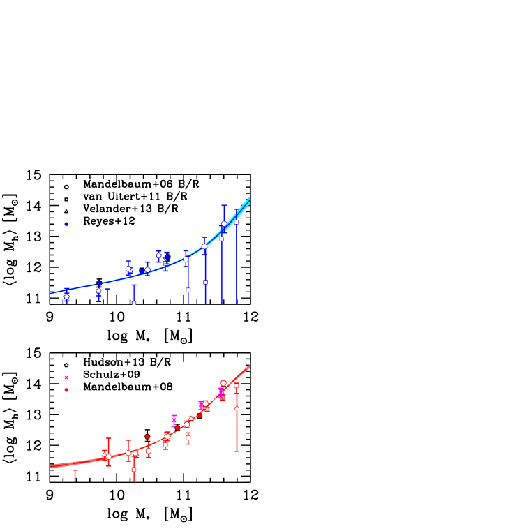
Figure 11.— Halo mass as a function of stellar mass (inverse SHMR), similar to Fig. 10. Model results are compared with several galaxy-galaxy weak lensing studies indicated inside the panels.

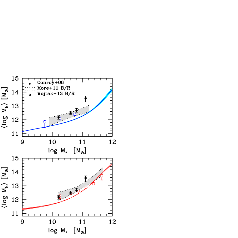
Figure 12.— Similar as Fig. 11 but this time comparing with several stacked satellite-kinematics studies indicated inside the panels.

In this subsection, we compare our constrained SHMRs for local blue and red central galaxies with those previously obtained using direct methods, namely galaxy-galaxy weak lensing and satellite kinematics. We also compare our average SHMR with those of previous semi-empirical studies. Where necessary, we apply corrections to the stellar mass reported by different authors to be consistent with the Chabrier (2003) IMF adopted here (see e.g., table 2 in Bernardi et al., 2010). When necessary, we also correct the halo masses to match our definition of virial mass. The corrections are done according to the relations reported in Appendix B.

5.4.1 Comparisons with direct methods

First, we compare our results with those obtained from galaxy-galaxy weak lensing. In these studies, in order to attain an acceptable signal-to-noise, observations of individual galaxies are stacked in bins of $M_{*}$ (or luminosity). Therefore, these measurements refer to halo mass as a function of $M_{*}$. In the upper and lower panels of Fig. 11, we reproduce our resulting $\langle\log\mbox{$M_{\rm h}$}\rangle(\mbox{$M_{*}$})$ relations for blue and red galaxies, respectively, as plotted in Fig. 10, and we compare them with several weak-lensing results. Note that in this case shaded areas represent the uncertainties around the SHMRs. Mandelbaum et al. (2006, empty blue circles, error bars are the 95% confidence intervals) used SDSS DR4 galaxies separated into late- and early-type galaxies according to the bulge-to-total ratio as given by the parameter frac_deV provided in the SDSS PHOTO pipeline (a de Vaucouleours/exponential decomposition was applied). van Uitert et al. (empty blue squares 2011) used the combined image data from the Red Sequence Cluster Survey (RCS2) and the SDSS DR7 to obtain the halo masses for late- and early-type galaxies as a function of $M_{*}$. (they also used the frac_deV parameter for defining the morphology). In the figure, we included measurements over only the redshift range $z=[0.08,0.41]$. Both Velander et al. (2014, empty blue triangles) and Hudson et al. (2013, empty blue pentagons) used the Canada-France-Hawaii Telescope Lensing Survey to derive halo masses of blue and red galaxies; the latter division was done based on the bimodality in the color–magnitude diagram. Halo mass measurements derived in Velander et al. (2014) are on average at redshift $z\sim 0.3$, while for Hudson et al. (2013) we have plotted only those measurements below $z=0.31$. We also plot the results from Mandelbaum, Seljak & Hirata (2008) (red solid circles) and Schulz, Mandelbaum & Padmanabhan (2010) (magenta crosses) for massive central early-type galaxies based on the local SDSS DR7 sample and a more sophisticated criteria for selecting early-type lens population.

Our SHMR determinations are consistent, within the uncertainties, with the various weak-lensing studies, which cover each one different mass ranges and have large uncertainties. As mentioned in Section 4, a source of discrepancy between different authors is due to the way blue and red (or late- and early-type) galaxies have been defined. In addition, results on $\langle\log\mbox{$M_{\rm h}$}\rangle$ as a function of $M_{*}$ are sensitive to the fact that different surveys may have different levels of measurement error in their stellar mass estimates, particularly those based on photometric surveys, (e.g., Leauthaud et al., 2012). In spite of all of these caveats, the overall agreement between these previous studies with our results is encouraging.

In Fig. 12, we compare our inverse SHMRs of blue and red centrals (as in Fig. 11) with stacked satellite kinematics studies. More et al. (2011, shaded gray area) used the Yang et al. (2007) group catalog and the spectroscopic velocities of the SDSS survey. Wojtak & Mamon (2013, open circles) used the SDSS DR7 spectroscopic catalog for blue and red central galaxies. We also plot the results by Conroy et al. (2007, solid circles), though these authors did not present their results for the $M_{\rm h}$-$M_{*}$ relation separated into blue and red galaxies (then, their data are repeated in the upper and lower panels); they combined data from the DEEP2 Galaxy Redshift Survey and the SDSS DR4 (their halo masses have been corrected by $\sim 30\%$ due to incompleteness, see their Appendix A). As seen, the satellite kinematics method tends to give higher halo masses than our semi-empirical results and than weak-lensing studies. The discrepancy between satellite kinematics and other methods has been noted previously, (see e.g., More et al., 2011; Skibba et al., 2011; Rodríguez-Puebla et al., 2011). The differences can be partially explained by the relation between $M_{\rm h}$ and the number of satellite galaxies at a fixed $M_{*}$. Since the technique is based on the kinematics of satellites, these studies can be biased to higher halo masses due to the loss of data in the case of those systems lacking satellites or with poor kinematical information, namely those of smaller halo masses at a given stellar mass.

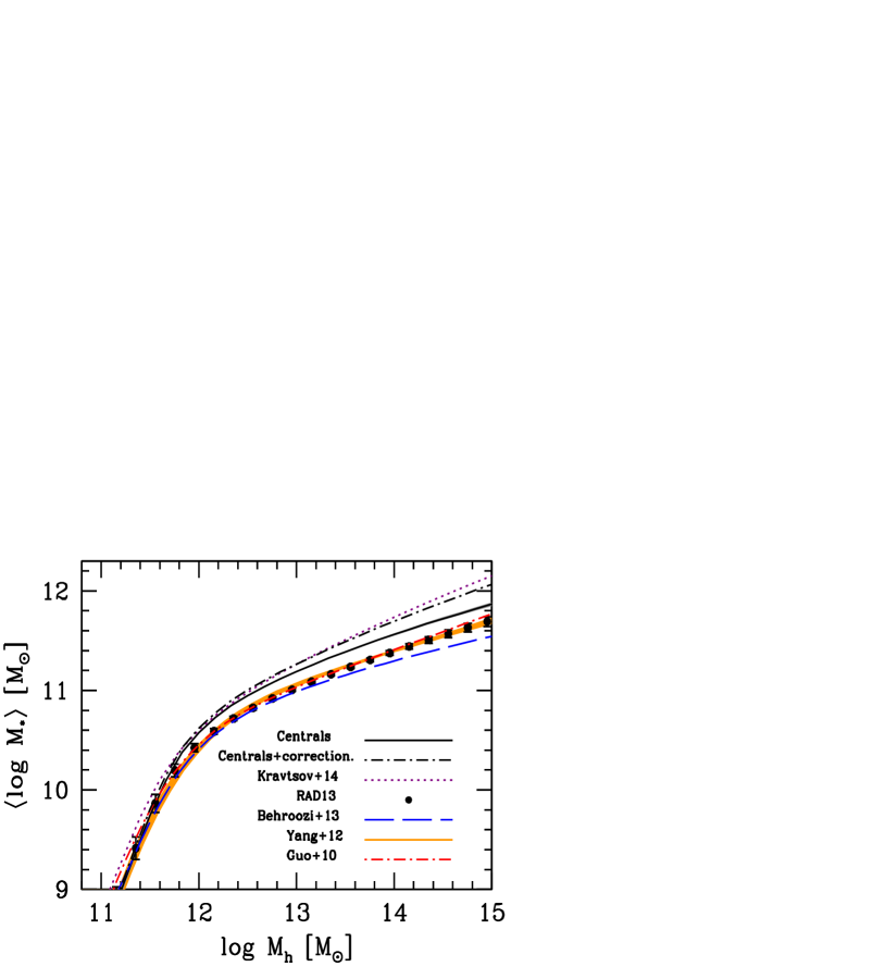
Figure 13.— Average SHMR for all central galaxies constrained by our method (see Eq. 17). This is indicated with the solid line surrounded by a gray shaded area which shows the model uncertainty around this relation. For comparison, the results obtained in Guo et al. (2010, red long-dashed curve), Behroozi, Wechsler & Conroy (2013, blue dot-dashed curve), Y12(orange shaded area indicate their 68% of confidence), and RAD13 (dots with error bars) are reproduced. In addition, we plot our resulting SHMR for all central galaxies that takes into account more adequate light profile fittings to galaxies (black long-dotted curve). This is compared with the SHMR for all galaxies reported in Kravtsov, Vikhlinin & Meshscheryakov (2014, violet dotted lines).

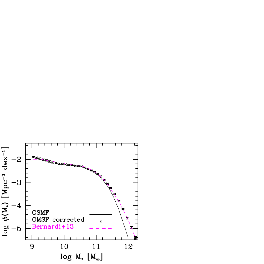
Figure 14.— GSMF as inferred in Section 3 but introducing a correction on the stellar masses due to new light profile fittings to galaxies, skeletal symbols with error bars. The magenta short dashed line line shows the GSMF reported in Bernardi et al. (2013), who calculated stellar masses with the new light profile fittings (see text for details). For comparison, the solid line shows the GSMF for all galaxies from the MPA-JHU NYU-VAGC/SDSS DR7 sample obtained in Section 3.

5.4.2 Comparison with previous inferences of the average SHMR

Figure 13 compares the average SHMR of central galaxies (Eq. 17) constrained by our method with those reported in Guo et al. (2010, red long-dashed curve), Behroozi, Wechsler & Conroy (2013, blue dot-dashed curve), Y12 (orange shaded area indicate their 68% of confidence), and RAD13 (dots with error bars). In the first two works, the SHMR was obtained by matching the abundances of all galaxies to the abundances of halos plus subhalos, therefore, it is rather the SHMR of all galaxies. Instead, in the case of the last works, their SHMRs are only for central galaxies (their set SMF2 and set C, respectively). The SHMR of central and all galaxies do not differ actually too much because the SHMR of satellite galaxies is close to the one of central galaxies (RAD13).

At masses below $\mbox{$M_{\rm h}$}\sim 10^{12}$ M_⊙, our average (blue + red galaxies) SHMR for centrals is close to the SHMRs reported in the above cited studies. In contrast, at larger masses, our SHMR increases more rapidly than these studies. The main reason is that at large masses our calculation of the GSMF falls slightly shallower than in previous works, see Fig.2. However, it could be that the high-mass end of the GSMF is even shallower than our determination!

Recently, several studies have pointed out to a systematical underestimation of luminosity and stellar mass-to-light ratios of galaxies due to the commonly used aperture limits in the SDSS (see Bernardi et al., 2013, and more references therein; see also Mendel et al. 2014). Surface brightness (mass) profiles of galaxies, in particular the central ones in clusters, extends much further away than the commonly used apertures (Kravtsov, Vikhlinin & Meshscheryakov, 2014, and more references therein). In Bernardi et al. (2013), luminosity and stellar mass functions were calculated based on different model fits for the surface brightness profiles in the SDSS galaxies. The authors showed that their results preferred GSMFs with the most luminous galaxies having larger masses for a given number density than most of the previous published GSMFs. Similar conclusion were obtained in He et al. (2013) based on a more sophisticated photometric data reduction from the SDSS DR7 and with morphological classifications from the Galaxy Zoo project (Lintott et al., 2011). Kravtsov, Vikhlinin & Meshscheryakov (2014) have confirmed this by using a compilation of well studied massive central cluster galaxies. Mendel et al. (2014) have compared the MPA-JHU DR7 stellar masses with the ones obtained by computing accurate bulge+disk and Sérsic profile photometric decompositions in several bands. In the case of Sérsic profile, they find masses larger by $\approx 0.08$ dex at the smallest masses and by $\approx 0.23$ dex at the largest masses. Following their results, we correct conservatively our masses by $\approx 0.05$ dex for masses up to log($M_{*}$/M_⊙)$\sim 10.7$ and then increase smoothly the correction ending with 0.23 dex at log($M_{*}$/M_⊙)$\sim 12$.

In Fig. 14, we reproduce the resulting total GSMF by correcting stellar masses as described above (skeletal symbols with error bars). For comparison, in the same figure we include the GSMF for all galaxies from the MPA-JHU NYU-VAGC/SDSS DR7 sample obtained in Section 3, solid line. The corrected GSMF is consistent with previous estimates, except at the high-mass end, which has a significantly shallower fall than most of previous ones, but in good agreement with Bernardi et al. (2013, their Sérsic profile case for the $M_{*}$ estimate, magenta short dashed line). These authors extensively discuss about how sensitive is the mass determination of the most luminous galaxies on the way the light profile is fitted. The spirit of the correction introduced above to our stellar masses was namely to take into account more adequate light profile fittings to galaxies, specially the most massive ones, as was done in Bernardi et al. (2013).

In Figure 13 we plot the resulting SHMR for all central galaxies when using the corrected stellar masses (black long-dotted curve). For comparison we also reproduce the SHMR for all galaxies reported in Kravtsov, Vikhlinin & Meshscheryakov (2014, violet dotted lines). Both results are similar and they show that when taking into account more adequate light-profile fittings to galaxies, specially the most massive ones, the SHMR increases more rapidly than previous reports. However, we highlight that all the results presented in previous sections we used a GSMF estimated based on the SDSS standard light-profile fittings, see Section 3.1.

6. Summary and Conclusions

By means of a semi-empirical galaxy-halo connection model, we have inferred the SHMRs of local blue and red central galaxies as well as their intrinsic scatters. The SHMR of all central galaxies is the density average of these SHMRs. Our parametric model is a combination of the SHAM, HOD model and CSMF formalism. The model allows us to separate the fraction of halos hosting blue/red central galaxies at each halo mass. The parameters of the model were constrained by using the GSMFs of blue and red galaxies inferred here from the SDSS DR7, divided into central and satellite components according to the Y12 galaxy group catalog, and the correlation functions of blue and red galaxies in different $M_{*}$ bins (Li et al., 2006). The criterion of the latter authors, based on the color–magnitude diagram, is used to separate the samples into blue and red galaxies. The main results obtained with our semi-empirical approach are as follows:

$\bullet$ The mean SHMR of blue and red central galaxies are different at a significant statistical level. At a given $M_{\rm h}$, blue centrals have larger $M_{*}$ than red centrals. At log($M_{\rm h}$/M_⊙)$\approx 11.7$, the difference attains its minimum, $0.16$ dex. At larger masses, it increases up to $0.24$ dex for log($M_{\rm h}$/M_⊙)$\approx 12.7$, remaining then roughly constant. At smaller masses, the difference strongly increases. These differences are larger than the $1\sigma$ confidence levels of each relation and their corresponding constrained scatters. The $M_{*}$-to-$M_{\rm h}$ ratio of blue (red) centrals peaks at log($M_{\rm h}$/M_⊙)$\approx 12.17$ ($\approx 12$) with a mean value of 0.051 (0.031).

$\bullet$ The density-averaged SHMR for all central galaxies lies in between the SHMR of blue and red galaxies, but closer to the former at log($M_{\rm h}$/M_⊙)$<11.5$ and closer to the latter at log($M_{\rm h}$/M_⊙)$>12.5$. This is because blue and red central galaxies dominate below and above these masses, respectively. At the mass interval $11.5\lower 2.15277pt\hbox{$\;\buildrel<\over{\sim}\;$}$ log($M_{\rm h}$/M_⊙)$\lower 2.15277pt\hbox{$\;\buildrel<\over{\sim}\;$}12.5$, the conditional stellar mass distribution (scatter) of central galaxies is strongly bimodal and color dependent.

$\bullet$ The constrained scatters around the blue/red/average SHMRs are small. The width of the assumed lognormal function for the conditional stellar mass distribution (scatter) is slightly smaller for blue centrals than for red centrals: $\sigma_{b}\approx 0.12$ dex and $\sigma_{r}\approx 0.14$ dex, respectively. Note that the values constrained for these scatters are composed by an intrinsic component and by a measurement error component.

$\bullet$ The scatter of the average SHMR changes from $0.20$ dex to $0.14$ dex for $\log(\mbox{$M_{\rm h}$}/\mbox{M${}_{\odot}$})\sim 11.3$ to $\log(\mbox{$M_{\rm h}$}/\mbox{M${}_{\odot}$})\sim 15$, respectively (the intrinsic scatter component is expected to be smaller). The increasing towards lower masses is due to the color bimodality in the conditional $M_{*}$ distribution at these masses. In previous studies, the scatter for all central galaxies has been assumed constant.

$\bullet$ The model predicts other distributions of the galaxy central and satellite populations, for both blue and red galaxies, which agree with independent observational determinations Among them, we remark:

1. The dependence of the blue/red central galaxy fractions on $M_{\rm h}$. We have assumed a functionality for this dependence based on observational studies, and with our method the free-parameters of this functionality were constrained. At log($M_{\rm h}$/M_⊙)$=11$, around $\approx 87\%$ of centrals are blue; this fraction decreases with $M_{\rm h}$; at log($M_{\rm h}$/M_⊙)$=11.83$ half of centrals are blue and half are red; for group masses, log($M_{\rm h}$/M_⊙)$>13$, the centrals are red in more than 90% of the cases. These results agree with weak lensing determinations.

2. The satellite population is dominated by blue galaxies in low mass halos, where blue galaxies also dominate among the central population. In contrast, red satellites dominate in massive halos, where red galaxies also dominate among centrals. The predicted satellite CSMFs for $M_{\rm h}$$\;\buildrel>\over{\sim}\;$$10^{13}$ M_⊙ agree well with those from the observational galaxy group catalog of Y12 (see also Yang, Mo & van den Bosch, 2009a).

Our findings show that blue central galaxies have higher $M_{*}$-to-$M_{\rm h}$ ratios than red centrals. However, this does not mean that the former have more efficient SF rate histories than the latter. Instead, this can be interpreted as that red centrals are such because they halted their $M_{*}$ growth in the past, likely by SF quenching processes. Such an interpretation is better seen in the inverse SHMR, which shows that for a given $M_{*}$, red centrals reside in more massive halos than blue centrals. This is likely because the stellar mass growth of red centrals is halted (mainly due to quenching) while their halos continue growing hierarchically. Since the difference in $M_{\rm h}$ between red and blue galaxies increases with $M_{*}$, the quenching redshift is expected to happen earlier as the galaxy is more massive (downsizing). That red galaxies have on average more massive halos than blue one at a given $M_{*}$, implies also that the former are more clustered than the latter, as observations show.

Appendix A A. K-correction

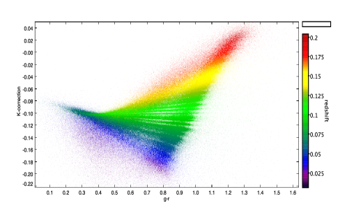
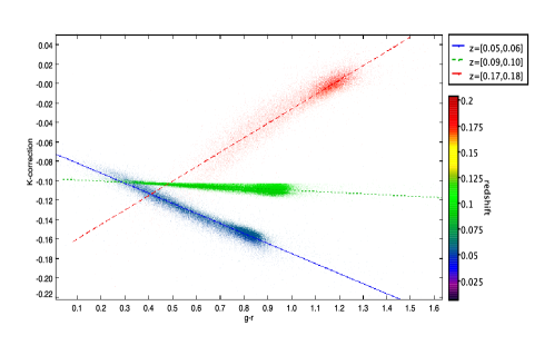
Figure 15.— Left panel: K-correction from the NYU-VAGC (Blanton et al., 2005) as a function of $(g-r)$ color and redshift. Right panel: The same as left panel but for three different redshifts bins. The different lines show the best fits for a relation of the form $K(g-r)=m\times(g-r)-b$ for these redshifts bins.

In this Appendix, we describe our analytical model for the K-correction. Figure 15 shows the K-correction (to $z=0.1$) as a function of $(g-r)$ colors (to $z=0.0$) and redshift. Recall that our redshift range is $0.01\leq z\leq 0.20$. For this plot, we use the values of the K-corrections reported in the NYU-VAGC (Blanton et al., 2005) based on the SDSS DR7 and calculated for each galaxy from the k-correction program v$4\_1\_4$ (Blanton & Roweis, 2007). As can be seen in right hand panel, for a given interval of redshift the relation between the K-correction and color is very well approximated to a linear relation, i.e., $K(g-r)=a\times(g-r)-b$. By dividing our redshift range into 20 redshift bins of width 0.01, we have found that the color and redshift dependence of the K-correction to $z=0.1$ is

$$K(z,g-r)=a(z)\times(g-r)-b(z);$$ (A1)

where

$$a(z)=\left\{\begin{array}[]{rcl}-1.649\log(1+z)-0.093&{\rm for}&z\leq 0.045\\ 5.590\log(1+z)-0.231&{\rm for}&z>0.045,\\ \end{array}\right.$$ (A2)

and

$$b(z)=\left\{\begin{array}[]{rcl}6.276\log(1+z)-0.181&{\rm for}&z\leq 0.045\\ -2.303\log(1+z)-0.017&{\rm for}&z>0.045.\\ \end{array}\right.$$ (A3)

The above approximation recovers, on average, to $\sim 10\%$, and $\sim 1\%$ the values of the K-correction and absolute magnitudes, respectively.

Appendix B B. Halo mass transformations

In order to find the differences in halo mass depending on the different definitions of it, we employed halo catalogs from the Bolshoi simulation (Klypin, Trujillo-Gomez & Primack, 2011), where halos are identified by means of the Bound-Density Maxima halo finder algorithm (Klypin & Holtzman, 1997). The advantage of using these catalogs is that they report masses based on different definitions of halo mass, so we can use them in order to obtain average correlations between these mass definitions. To do so, we use a sample of $\sim 94,000$ halos. We find the following relations for the virial halo mass used here ($\mbox{$M_{\rm h}$}\equiv M_{\Delta_{\rm vir}}$):

$$\log(M_{\Delta_{\rm vir}}/\mbox{M${}_{\odot}$})=1.014\log(M_{\Delta_{m}}/\mbox{M${}_{\odot}$})-0.07,$$ (B1)

and

$$\log(M_{\Delta_{\rm vir}}/\mbox{M${}_{\odot}$})=0.98\log(M_{\Delta_{\rm crit}}/\mbox{M${}_{\odot}$})+0.21,$$ (B2)

where $\Delta_{m}=200$ and $\Delta_{\rm crit}=200$ are 200 times the mean matter and critical densities, respectively.

Appendix C C. Probability distributions

In Fig. 16 we show the 1D (diagonal) and 2D posterior distributions of the model parameters as constrained in Section 4. Note that in most of cases the constrained parameters do not correlate significantly among them.

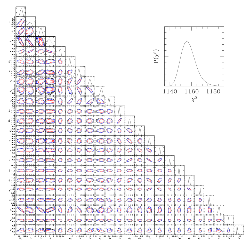
Figure 16.— Posterior probability distributions of our model parameters. Black contours represent the $90\%$ of the models with the lowest $\chi^{2}$, while blue and red contours are the same but for $68\%$ and $10\%$ of the models.

References

- Abbas & Sheth (2006) Abbas U., Sheth R. K., 2006, MNRAS, 372, 1749
- Baldry et al. (2012) Baldry I. K. et al., 2012, MNRAS, 421, 621
- Baldry et al. (2004) Baldry I. K., Glazebrook K., Brinkmann J., Ivezić Ž., Lupton R. H., Nichol R. C., Szalay A. S., 2004, ApJ, 600, 681
- Baldry, Glazebrook & Driver (2008) Baldry I. K., Glazebrook K., Driver S. P., 2008, MNRAS, 388, 945
- Behroozi, Conroy & Wechsler (2010) Behroozi P. S., Conroy C., Wechsler R. H., 2010, ApJ, 717, 379
- Behroozi, Wechsler & Conroy (2013) Behroozi P. S., Wechsler R. H., Conroy C., 2013, ApJ, 770, 57
- Bell et al. (2003) Bell E. F., McIntosh D. H., Katz N., Weinberg M. D., 2003, ApJS, 149, 289
- Bell et al. (2007) Bell E. F., Zheng X. Z., Papovich C., Borch A., Wolf C., Meisenheimer K., 2007, ApJ, 663, 834
- Berlind & Weinberg (2002) Berlind A. A., Weinberg D. H., 2002, ApJ, 575, 587
- Bernardi et al. (2013) Bernardi M., Meert A., Sheth R. K., Vikram V., Huertas-Company M., Mei S., Shankar F., 2013, MNRAS, 436, 697
- Bernardi et al. (2010) Bernardi M., Shankar F., Hyde J. B., Mei S., Marulli F., Sheth R. K., 2010, MNRAS, 404, 2087
- Blanton et al. (2003) Blanton M. R. et al., 2003, ApJ, 592, 819
- Blanton et al. (2005) Blanton M. R., Lupton R. H., Schlegel D. J., Strauss M. A., Brinkmann J., Fukugita M., Loveday J., 2005, ApJ, 631, 208
- Blanton & Moustakas (2009) Blanton M. R., Moustakas J., 2009, ARA&A, 47, 159
- Blanton & Roweis (2007) Blanton M. R., Roweis S., 2007, AJ, 133, 734
- Brinchmann et al. (2004) Brinchmann J., Charlot S., White S. D. M., Tremonti C., Kauffmann G., Heckman T., Brinkmann J., 2004, MNRAS, 351, 1151
- Bundy et al. (2006) Bundy K. et al., 2006, ApJ, 651, 120
- Bundy et al. (2010) Bundy K. et al., 2010, ApJ, 719, 1969
- Cacciato et al. (2009) Cacciato M., van den Bosch F. C., More S., Li R., Mo H. J., Yang X., 2009, MNRAS, 394, 929
- Chabrier (2003) Chabrier G., 2003, PASP, 115, 763
- Conroy, Gunn & White (2009) Conroy C., Gunn J. E., White M., 2009, ApJ, 699, 486
- Conroy et al. (2007) Conroy C. et al., 2007, ApJ, 654, 153
- Conroy & Wechsler (2009) Conroy C., Wechsler R. H., 2009, ApJ, 696, 620
- Conroy, Wechsler & Kravtsov (2006) Conroy C., Wechsler R. H., Kravtsov A. V., 2006, ApJ, 647, 201
- Cooray (2006) Cooray A., 2006, MNRAS, 365, 842
- Cooray & Sheth (2002) Cooray A., Sheth R., 2002, PhR, 372, 1
- Drory & Alvarez (2008) Drory N., Alvarez M., 2008, ApJ, 680, 41
- Drory et al. (2009) Drory N. et al., 2009, ApJ, 707, 1595
- Firmani & Avila-Reese (2010) Firmani C., Avila-Reese V., 2010, ApJ, 723, 755
- Fontanot et al. (2009) Fontanot F., De Lucia G., Monaco P., Somerville R. S., Santini P., 2009, MNRAS, 397, 1776
- Foucaud et al. (2010) Foucaud S., Conselice C. J., Hartley W. G., Lane K. P., Bamford S. P., Almaini O., Bundy K., 2010, MNRAS, 406, 147
- Gott et al. (2005) Gott, III J. R., Jurić M., Schlegel D., Hoyle F., Vogeley M., Tegmark M., Bahcall N., Brinkmann J., 2005, ApJ, 624, 463
- Guo et al. (2010) Guo Q., White S., Li C., Boylan-Kolchin M., 2010, MNRAS, 404, 1111
- Hartley et al. (2013) Hartley W. G. et al., 2013, MNRAS, 431, 3045
- He et al. (2013) He Y. Q., Xia X. Y., Hao C. N., Jing Y. P., Mao S., Li C., 2013, ApJ, 773, 37
- Hearin et al. (2013) Hearin A. P., Zentner A. R., Berlind A. A., Newman J. A., 2013, MNRAS, 433, 659
- Hogg (1999) Hogg D. W., 1999, ArXiv Astrophysics e-prints
- Hopkins et al. (2008) Hopkins P. F., Cox T. J., Kereš D., Hernquist L., 2008, ApJS, 175, 390
- Hudson et al. (2013) Hudson M. J. et al., 2013, ArXiv e-prints
- Jin et al. (2014) Jin S.-W., Gu Q., Huang S., Shi Y., Feng L.-L., 2014, ArXiv e-prints
- Jing, Mo & Börner (1998) Jing Y. P., Mo H. J., Börner G., 1998, ApJ, 494, 1
- Kauffmann et al. (2003) Kauffmann G. et al., 2003, MNRAS, 341, 33
- Klypin & Holtzman (1997) Klypin A., Holtzman J., 1997, ArXiv Astrophysics e-prints
- Klypin, Trujillo-Gomez & Primack (2011) Klypin A. A., Trujillo-Gomez S., Primack J., 2011, ApJ, 740, 102
- Knebe et al. (2013) Knebe A. et al., 2013, MNRAS, 435, 1618
- Kravtsov, Vikhlinin & Meshscheryakov (2014) Kravtsov A., Vikhlinin A., Meshscheryakov A., 2014, ArXiv e-prints
- Kravtsov et al. (2004) Kravtsov A. V., Berlind A. A., Wechsler R. H., Klypin A. A., Gottlöber S., Allgood B., Primack J. R., 2004, ApJ, 609, 35
- Leauthaud et al. (2012) Leauthaud A. et al., 2012, ApJ, 744, 159
- Li et al. (2012) Li C., Jing Y. P., Mao S., Han J., Peng Q., Yang X., Mo H. J., van den Bosch F., 2012, ApJ, 758, 50
- Li et al. (2006) Li C., Kauffmann G., Jing Y. P., White S. D. M., Börner G., Cheng F. Z., 2006, MNRAS, 368, 21
- Li & White (2009) Li C., White S. D. M., 2009, MNRAS, 398, 2177
- Lintott et al. (2011) Lintott C. et al., 2011, MNRAS, 410, 166
- Maller et al. (2009) Maller A. H., Berlind A. A., Blanton M. R., Hogg D. W., 2009, ApJ, 691, 394
- Mandelbaum, Seljak & Hirata (2008) Mandelbaum R., Seljak U., Hirata C. M., 2008, JCAP, 8, 6
- Mandelbaum et al. (2006) Mandelbaum R., Seljak U., Kauffmann G., Hirata C. M., Brinkmann J., 2006, MNRAS, 368, 715
- Mendel et al. (2014) Mendel J. T., Simard L., Palmer M., Ellison S. L., Patton D. R., 2014, ApJS, 210, 3
- Mo, van den Bosch & White (2010) Mo H., van den Bosch F. C., White S., 2010, Galaxy Formation and Evolution
- More et al. (2011) More S., van den Bosch F. C., Cacciato M., Skibba R., Mo H. J., Yang X., 2011, MNRAS, 410, 210
- Moustakas et al. (2013) Moustakas J. et al., 2013, ApJ, 767, 50
- Muñoz-Cuartas et al. (2011) Muñoz-Cuartas J. C., Macciò A. V., Gottlöber S., Dutton A. A., 2011, MNRAS, 411, 584
- Neistein et al. (2011) Neistein E., Li C., Khochfar S., Weinmann S. M., Shankar F., Boylan-Kolchin M., 2011, MNRAS, 416, 1486
- Papastergis et al. (2012) Papastergis E., Cattaneo A., Huang S., Giovanelli R., Haynes M. P., 2012, ApJ, 759, 138
- Peng & et al. (2010) Peng Y.-j., et al., 2010, ApJ, 721, 193
- Peng et al. (2012) Peng Y.-j., Lilly S. J., Renzini A., Carollo M., 2012, ApJ, 757, 4
- Pozzetti et al. (2010) Pozzetti L. et al., 2010, A&A, 523, A13
- Reddick et al. (2013) Reddick R. M., Wechsler R. H., Tinker J. L., Behroozi P. S., 2013, ApJ, 771, 30
- Rodríguez-Puebla, Avila-Reese & Drory (2013) Rodríguez-Puebla A., Avila-Reese V., Drory N., 2013, ApJ, 767, 92
- Rodríguez-Puebla et al. (2011) Rodríguez-Puebla A., Avila-Reese V., Firmani C., Colín P., 2011, RMxAA, 47, 235
- Rodríguez-Puebla, Drory & Avila-Reese (2012) Rodríguez-Puebla A., Drory N., Avila-Reese V., 2012, ApJ, 756, 2
- Schulz, Mandelbaum & Padmanabhan (2010) Schulz A. E., Mandelbaum R., Padmanabhan N., 2010, MNRAS, 408, 1463
- Shankar et al. (2006) Shankar F., Lapi A., Salucci P., De Zotti G., Danese L., 2006, ApJ, 643, 14
- Sheth et al. (2001) Sheth R. K., Hui L., Diaferio A., Scoccimarro R., 2001, MNRAS, 325, 1288
- Skibba & Sheth (2009) Skibba R. A., Sheth R. K., 2009, MNRAS, 392, 1080
- Skibba et al. (2011) Skibba R. A., van den Bosch F. C., Yang X., More S., Mo H., Fontanot F., 2011, MNRAS, 410, 417
- Smith et al. (2003) Smith R. E. et al., 2003, MNRAS, 341, 1311
- Thomas et al. (2005) Thomas D., Maraston C., Bender R., Mendes de Oliveira C., 2005, ApJ, 621, 673
- Tinker et al. (2008) Tinker J., Kravtsov A. V., Klypin A., Abazajian K., Warren M., Yepes G., Gottlöber S., Holz D. E., 2008, ApJ, 688, 709
- Tinker et al. (2013) Tinker J. L., Leauthaud A., Bundy K., George M. R., Behroozi P., Massey R., Rhodes J., Wechsler R. H., 2013, ApJ, 778, 93
- Tinker et al. (2010) Tinker J. L., Robertson B. E., Kravtsov A. V., Klypin A., Warren M. S., Yepes G., Gottlöber S., 2010, ApJ, 724, 878
- Tinker et al. (2005) Tinker J. L., Weinberg D. H., Zheng Z., Zehavi I., 2005, ApJ, 631, 41
- Tinker & Wetzel (2010) Tinker J. L., Wetzel A. R., 2010, ApJ, 719, 88
- Tomczak et al. (2014) Tomczak A. R. et al., 2014, ApJ, 783, 85
- Vale & Ostriker (2004) Vale A., Ostriker J. P., 2004, MNRAS, 353, 189
- Vale & Ostriker (2008) Vale A., Ostriker J. P., 2008, MNRAS, 383, 355
- van den Bosch et al. (2008) van den Bosch F. C., Aquino D., Yang X., Mo H. J., Pasquali A., McIntosh D. H., Weinmann S. M., Kang X., 2008, MNRAS, 387, 79
- van den Bosch, Yang & Mo (2003) van den Bosch F. C., Yang X., Mo H. J., 2003, MNRAS, 340, 771
- van den Bosch et al. (2007) van den Bosch F. C. et al., 2007, MNRAS, 376, 841
- van Uitert et al. (2011) van Uitert E., Hoekstra H., Velander M., Gilbank D. G., Gladders M. D., Yee H. K. C., 2011, A&A, 534, A14
- Velander et al. (2014) Velander M. et al., 2014, MNRAS, 437, 2111
- Wake, Franx & van Dokkum (2012) Wake D. A., Franx M., van Dokkum P. G., 2012, ArXiv e-prints
- Wang et al. (2004) Wang Y., Yang X., Mo H. J., van den Bosch F. C., Chu Y., 2004, MNRAS, 353, 287
- Watson, Berlind & Zentner (2011) Watson D. F., Berlind A. A., Zentner A. R., 2011, ApJ, 738, 22
- Watson & Conroy (2013) Watson D. F., Conroy C., 2013, ArXiv e-prints
- Weinmann et al. (2006) Weinmann S. M., van den Bosch F. C., Yang X., Mo H. J., 2006, MNRAS, 366, 2
- Wojtak & Mamon (2013) Wojtak R., Mamon G. A., 2013, MNRAS, 428, 2407
- Woo et al. (2013) Woo J. et al., 2013, MNRAS, 428, 3306
- Yang, Mo & van den Bosch (2003) Yang X., Mo H. J., van den Bosch F. C., 2003, MNRAS, 339, 1057
- Yang, Mo & van den Bosch (2008) Yang X., Mo H. J., van den Bosch F. C., 2008, ApJ, 676, 248
- Yang, Mo & van den Bosch (2009a) Yang X., Mo H. J., van den Bosch F. C., 2009a, ApJ, 695, 900
- Yang, Mo & van den Bosch (2009b) Yang X., Mo H. J., van den Bosch F. C., 2009b, ApJ, 693, 830
- Yang et al. (2013) Yang X., Mo H. J., van den Bosch F. C., Bonaca A., Li S., Lu Y., Lu Y., Lu Z., 2013, ApJ, 770, 115
- Yang et al. (2007) Yang X., Mo H. J., van den Bosch F. C., Pasquali A., Li C., Barden M., 2007, ApJ, 671, 153
- Yang et al. (2012) Yang X., Mo H. J., van den Bosch F. C., Zhang Y., Han J., 2012, ApJ, 752, 41
- Zehavi et al. (2011) Zehavi I. et al., 2011, ApJ, 736, 59
- Zehavi et al. (2005) Zehavi I. et al., 2005, ApJ, 630, 1
- Zheng et al. (2005) Zheng Z. et al., 2005, ApJ, 633, 791