Can Natural Sunlight Induce Coherent Exciton Dynamics?

Abstract

Excitation of a model photosynthetic molecular aggregate by incoherent sunlight is systematically examined. For a closed system, the excited state coherence induced by the sunlight oscillates with an average amplitude that is inversely proportional to the excitonic gap, and reaches a stationary amplitude that depends on the temperature and coherence time of the radiation field. For an open system, the light-induced dynamical coherence relaxes to a static coherence determined by the non-canonical thermal distribution resulting from the entanglement with the phonon bath. The decay of the excited state population to the common ground state establishes a non-equilibrium steady-state flux driven by the sunlight, and it defines a time window to observe the transition from dynamical to static coherence. For the parameters relevant to photosynthetic systems, the exciton dynamics initiated by the sunlight exhibits a non-negligible amount of dynamical coherence (quantum beats) on the sub-picosecond timescale; however, this sub-picosecond time-scale is long enough for light-harvesting systems to establish static coherence, which plays a crucial role in efficient energy transfer. Further, a relationship is established between the non-equilibrium steady-state induced by the sunlight and the coherent dynamics initiated from the ground state by a laser $\delta$-pulse, thereby making a direct connection between incoherent sunlight excitation and ultrafast spectroscopy.

I Introduction

Recent developments in 2D electronic spectroscopy (2DES) of molecular aggregates have demonstrated the presence of coherent dynamics in the electronic degrees of freedom (DOF), known as electronic coherence, as opposed to the expected incoherent hopping dynamics. 2DES was first used in the Fleming group to measure long-lived oscillations in the Fenna-Matthews-Olson (FMO) photosynthetic pigment-protein complex, which reveals the presence of long-lived electronic coherence Engel2007a . This has led to a heated debate about its importance to the efficiency of the excitonic energy transfer in photosynthesis in general. Since then, long-lived coherence has been reported in many other systems Engel2007a ; Mercer2009a ; Collini2010a . The term quantum coherence, generally used to describe the off-diagonal elements of the density matrix in the exciton basis, can be associated with several physical phenomena. It is particularly important here to distinguish between a static coherence that remains constant for long times and corresponds to stationary effects in equilibrium states or non-equilibrium steady states (e.g., localization and entanglement with the bath), and a dynamical coherence, which is a transient effect associated with the time-evolution of the superposition of eigen states. The latter is related to the recently discovered quantum beats in 2DES measurements, which can be quantified as transient oscillations in the coherence term. The issue of sunlight-induced coherence refers to the ’dynamic coherence’ associated with the quantum beats; whereas the entanglement with the phonon or photon bath leads to ’static coherence’ associated with non-canonical thermal distributions.

One of the important questions in this discussion is whether electronic coherent dynamics can be initiated by natural sunlight Jiang1991a ; Mancal2010a . In 2DES or pump-probe experiments, molecules are excited by ultra-short femtosecond laser pulses which lead to a pure quantum state – generally in the form of a superposition of several locally excited states. On the other hand, natural thermal light is incoherent: In the semi-classical picture, it can be described as uncorrelated noise that leads to an excitation of populations, but not necessarily coherence. In the quantum picture, it was argued that the arrival of photons does not have to be localized at a particular time nor have a well-defined phase – the thermal light behaves more like a dissipative quantum bath at high temperature with a very short coherence time ($<10\;\mathrm{fs})$. Although there have been many models of the incoherent light excitation Jiang1991a ; Mancal2010a , the exact quantum description of the light, as well as a thorough analysis of its properties over a broad range of parameters, is still not available. This article aims to fill this gap. We use the Hierarchical Equations of Motion (HEOM) Tanimura1989a ; Ishizaki2009a ; Dijkstra2010 ; Moix2013 as a non-perturbative description of both the phonon bath and photon radiation. We further introduce a decay channel, which defines an observation window for the induced exciton dynamics. The Drude-Lorentz spectral density assumed by the HEOM differs from the black-body spectrum; however, in contrast to the classical approach, the HEOM correctly describes temperature effects and all the relevant quantum effects and allows us to examine the dependence of the induced dynamics on the coherence of the radiation field.

In the first part, we analyze the dynamics of a closed system pumped by incoherent light. The amount of dynamical coherence (i.e, the amplitude of oscillations) generated under sunlight pumping is constant, inversely proportional to the exciton energy gap, but decreases if normalized by the linearly growing exciton populations. We analyze the amount of dynamic coherence for different coherence times of the radiation and show that for very incoherent radiation, which is the case relevant for the natural sunlight, the white-noise model (WNM) provides a reliable description of the optical excitation. Open quantum systems allow the additional dephasing mechanism, which depends on the detailed properties of the system-bath coupling. Our analysis of the closed system aims to demonstrate that the presence of dynamical coherence is not excluded by the fact that solar light is incoherent, provided the additional dephasing of the electronic coherence from the phonon bath is sufficiently slow, as observed in many biological systems. Further analysis of the open system reveals the phonon-induced static coherence, which appears as the long time limit after the dynamic coherence is suppressed by the phonon noise.

In the second part, we include a decay channel which sets a time-scale for experimental observation on the individual molecule level. Physically, the decay channel can be interpreted as trapping at the reaction center, fluorescence emission, or non-radiative decay Cao2006 ; Shapiro2013 . The density matrix formalism is a general tool to evaluate experimental results in the framework of dissipative quantum dynamics. However, it does not necessarily tell us about the state of individual molecules, which is an issue closely related to the measurement problem in single molecule experiments. The statistical interpretation of the density matrix formalism offers a mechanism in which the pure quantum state of individual molecules can survive for long times, and the observed loss of coherence is attributed to ensemble averaging or time averaging, which results in cancelation of phase coherence in states with different quantum phases. This type of decoherence often applies to dynamical coherence. In contrast, because of the coupling to phonons, the coherence is lost even on the level of individual molecules after the trace over the bath is performed. This type of decoherence mainly applies to static coherence. We cannot differentiate these two types of coherence based on the density matrix description but can distinct them on the single molecule level, which will be further discussed in a future publication. For example, in ensemble measurements, there is not a particular event to set time zero in our experiment, and one thus has to be careful about the initial condition Cao2006 . We try to avoid these interpretational issues by introducing a decay channel, which introduces a natural time-scale for energy transfer and establish the non-equilibrium steady state. Then, the contribution of light-induced dynamical coherence to light-harvesting energy transfer is determined by the ratio of the dephasing time and decay time, and may not play a dominant role in light-harvesting systems, such as FMO or LH2.

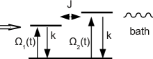
Figure 1: Schematic V-type model with two excited states and the common ground state, which are coupled with the radiation field of the sunlight, with independent phonon baths, and with a decay rate $k$ to the ground state. The excited states are coupled by a resonance constant $J$.

II Model and Methods

II.1 Molecular Dimer System

The system of interest is a molecular dimer in contact with sunlight and two independent phonon baths, which represent both vibrational DOF of the molecules and the nuclear DOF of the surrounding environment (see Fig. 1). This model captures the essential physics of delocalized exciton states and coherent exciton dynamics relevant for light-harvesting systems.

The molecular dimer system has been extensively studied in quantum information, quantum optics, and Förster energy transfer theory Moix2013 . Each molecule, denoted by an index $i\in\{1,2\}$, is either in its electronic ground state $|g_{i}\rangle$ or its electronic excited states $|e_{i}\rangle$ (i.e., excitons). For convenience, we introduce the composite states $|\bar{g}\rangle=|g_{1}\rangle|g_{2}\rangle$, $|\bar{e}_{1}\rangle=|e_{1}\rangle|g_{2}\rangle$, $|\bar{e}_{2}\rangle=|g_{1}\rangle|e_{2}\rangle$ and $|\bar{f}\rangle=|e_{1}\rangle|e_{2}\rangle$. We remove the $|\bar{f}\rangle$-state from our model since its influence is negligible due to its high energy. Then, the molecular dimer can be described by the system Hamiltonian

$$\hat{H}_{S}=\begin{pmatrix}\epsilon_{1}&J&0\\ J&\epsilon_{2}&0\\ 0&0&\epsilon_{g}\\ \end{pmatrix}$$ (1)

where the energies of states $|\bar{e}_{1}\rangle$, $|\bar{e}_{2}\rangle$, $|\bar{g}\rangle$ are denoted $\epsilon_{1}$, $\epsilon_{2}$, $\epsilon_{g}$, respectively. The symbol $J$ denotes the exciton resonance-coupling. The two-level-system Hamiltonian in the excited state manifold can be diagonalized in the excitonic basis consisting of $|\bar{e}_{+}\rangle$ and $|\bar{e}_{-}\rangle$. Throughout this paper, we use the subscripts $\{1,2\}$ to denote the molecular (local) basis and subscripts $\{+,-\}$ to denote the excitonic basis, and consider the off-diagonal matrix element $\rho_{+-}$ in the excitonic basis as a measure of coherence. The typical parameters for light-harvesting systems are $\epsilon_{1}=9900\;\mathrm{cm}^{-1}$, $\epsilon_{2}=10000\;\mathrm{cm}^{-1}$, $\epsilon_{g}=0$, and $J=50\;\mathrm{cm}^{-1}$. For a closed system, the physical pictures for arbitrary $J$ are equivalent. Hence, we can simply take $J=0$ for convenience, without losing any generality

The light-matter interaction between the molecular dimer and the radiation field occurs via the dipole coupling, given by

$$~{}\hat{H}_{S-R} = -\hat{\mu}{\otimes}\hat{E}$$

$$= -\sum_{v=1,2}[\mu_{v}|\bar{e}_{v}\rangle\langle\bar{g}|+H.c.]{\otimes}\hat{E}$$

where $\hat{\mu}$ is the total transition dipole operator of the dimer, and $\hat{E}$ is the radiation field, which are briefly discussed in the Appendix A. In order to simplify the formulation and unify the formalism with the phonon baths, we rewrite the light-matter interaction term as $\hat{H}_{S-R}=\hat{K}_{R}{\otimes}\hat{V}_{R}$, where $\hat{K}_{R}=\hat{\mu}/\mu$ and $\hat{V}_{R}=-\mu\hat{E}$. The constant $\mu=\frac{1}{2}\sqrt{\mathrm{Tr}\,\hat{{\mu}}\cdot\hat{{\mu}}}$ denotes the magnitude of the total dipole moment. The information about the electric field strength and the magnitude of the dipole moment is now incorporated into $\hat{V}_{R}$ and enters through the radiation reorganization energy $\lambda_{R}$ introduced later. For simplicity, dipoles are oriented in the direction of the radiation field so that the scalar form of the dipole interaction is adopted. The sunlight consists of photons, so its radiation field $\hat{E}$ or $\hat{V}_{R}$ is treated as a photon bath, which is fully characterized by the energy gap correlation function (EGCF)

$$C_{R}(t)=\langle\hat{V}_{R}(t)\hat{V}_{R}(0)\rangle.$$ (3)

The time-dependence of $\hat{V}_{R}(t)$ denotes the interaction picture with respect to the radiation field. We use the over-damped harmonic bath EGCF MukamelBook , i.e., the Drude-Lorentz spectral density, which is paramertized by the radiation temperature $T_{R}=6000\;\mathrm{K}$, cutoff frequency $\gamma_{R}=0.1\;\mathrm{fs}-1\;\mathrm{fs}^{-1})$ and reorganization energy $\lambda_{R}$ (see Appendix A). In the weak excitation regime, the excited state density matrix is proportional to $\lambda_{R}$, which can now be taken a normalization constant and needs not be specified. As this point, we have introduced the system Hamiltonian $\hat{H}_{S}$ and radiation-system interaction Hamiltonian $\hat{H}_{S-R}$, and thus have completely defined a closed dimer system pumped by sunlight.

Light-harvesting complexes are embedded in the protein environment and therefore are open systems coupled to phonon baths. This coupling destroys the dynamic coherence and is described as MayKuehnBook ; Olsina2010a

$$\hat{H}_{S-B}=\hat{V}_{1}|\bar{e}_{1}\rangle\langle\bar{e}_{1}|+\hat{V}_{2}|\bar{e}_{2}\rangle\langle\bar{e}_{2}|$$ (4)

where $\hat{V}_{n}$ is the interaction strength between the molecule and its phonon bath. Similar to the photon bath, we use the Drude-Lorentz phonon spectral density and define the EGCF as

$$C_{n}(t)=\langle\hat{V}_{n}(t)\hat{V}_{n}(0)\rangle,$$ (5)

where $\hat{V}_{n}(t)$ is a linear function of phonon operators expressed in the interaction picture with respect to the phonon bath. For simplicity, the phonon baths coupled to the two molecules share the same parameters: $T_{1}=T_{2}=300\;\mathrm{K}$, $\gamma_{1}=\gamma_{2}=100\;\mathrm{cm}^{-1}$, and $\lambda_{1}=\lambda_{2}$ in the range of $10\;\mathrm{cm}^{-1}-100\;\mathrm{cm}^{-1}$.

To calculate photon-coupling and phonon-coupling, we use the hierarchical equation of motion (HEOM), which are developed for the Debye-Lorentz spectral density. Details of HEOM can be found in the Appendix B. Because of the high-temperature and extremely short coherence time of the sunlight, the white noise description of the excitation by solar radiation is reliable, where the radiation field is treated classically. Hence, in absence of the exciton-phonon interaction, we have derived an analytical solution based on the Haken-Strobl model HakenStrobl1973 ; Cao2009 ; Wu2013 to describe the pumping by the sunlight. We present this white-noise model (WNM) in the following.

II.2 White Noise Model

The full quantum treatment of the incoherent light in the form of HEOM is computationally expensive. If the coherence time of the solar radiation is shorter than all other time-scales of the system dynamics, including the resonance coupling, the phonon bath time-scale, and the dephasing time, which is typical in photosynthesis, then the white-noise model (WNM) should be well applicable for the description of the radiation. In this model, the energy gap correlation function (EGCF) is expressed in the form

$$~{}C^{R}(t)=I^{R}\delta(t)\;,$$ (6)

where $I^{R}$ is a parameter representing coupling of the electric field to the given exciton transition. The quantum dynamics under this classical white noise is known as the Haken-Strobl model, which is exactly solvable in some cases, including the V-shape three-level system with a trap (see Cao2009 ). We can generalize the classical noise to quantum noise by evaluating the Redfield pumping rates given as

$$I_{+}^{R}= \frac{2\gamma_{R}\lambda_{R}\varepsilon_{+}(\coth(\beta_{R}\varepsilon_{+}/2)-1)}{\gamma_{R}^{2}+(\varepsilon_{+}/\hbar)^{2}}\;,$$ (7a)

$$I_{-}^{R}= \frac{2\gamma_{R}\lambda_{R}\varepsilon_{-}(\coth(\beta_{R}\varepsilon_{-}/2)-1)}{\gamma_{R}^{2}+(\varepsilon_{-}/\hbar)^{2}}\;,$$ (7b)

where $\varepsilon_{i}~{}(i=\pm)$ denote eigenstate energies and $\beta_{R}=1/(k_{b}T_{R})$. In the weak field regime, $I^{R}\ll k$, the pumping creates no more than one excitation at any given time such that $\rho_{\bar{g}\bar{g}}\approx 1$. Then, the solution to the WNM is explicitly written as

$$\rho_{++}(t)= \frac{\mu_{+}^{2}I_{+}^{R}}{k\mu^{2}}(1-e^{-kt})\;,$$ (8a)

$$\rho_{--}(t)= \frac{\mu_{-}^{2}I_{-}^{R}}{k\mu^{2}}(1-e^{-kt})\;,$$ (8b)

$$\rho_{+-}(t)= \frac{\mu_{+}\mu_{-}}{\mu^{2}}\frac{({I_{+}^{R}+I_{-}^{R}})/2}{k+\frac{i}{\hbar}(\varepsilon_{+}-\varepsilon_{-})}(1-e^{-\frac{i}{\hbar}(\varepsilon_{+}-\varepsilon_{-})t-kt})\;.$$ (8c)

where all parameters are given in the excitonic basis. As long as the decay rates from the two molecules are identical and the dimer system is not coupled to any phonon bath, the above solution retains the same functional form for arbitrary inter-site coupling $J$. This is exactly the reason that the local and excitonic basis sets are equivalent for a closed system and the excitonic coupling $J$ does not change the physics. The detail derivation can be obtained in the Appendix C.

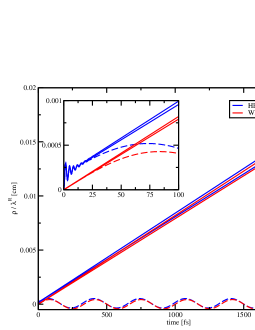
Figure 2: Dynamics of a molecular dimer with parameters $J=0,\epsilon_{1}=9900\;\mathrm{cm}^{-1},\epsilon_{2}=10000\;\mathrm{cm}^{-1}$ pumped by weak radiation characterized by parameters $T_{R}=6000\;\mathrm{K},\gamma_{R}=0.2\;\mathrm{fs}^{-1}$ according to the HEOM and WNM respectively. Populations (full lines) and real part of the coherence (dashed lines) are plotted. Apart from the transient effects at short time shown in the inset, both models give similar results.

Table 1: Pumping rates $p_{+}$ and $p_{-}$ in units of the reorganization energy according to the HEOM and WNM models for a closed system pumped by incoherent light. Parameters of the system are described in the caption of Fig. 2. The small differences may be explained by the Markov approximation.

pumping rate	HEOM	WNM
$p_{+}/\lambda_{R}$	$8.25\cdot 10^{-6}\;\mathrm{cm}\;\mathrm{fs^{-1}}$	$8.20\cdot 10^{-6}\;\;\mathrm{cm}\;\mathrm{fs^{-1}}$
$p_{-}/\lambda_{R}$	$7.91\cdot 10^{-6}\mathrm{\;\mathrm{cm}\;\mathrm{fs^{-1}}}$	$7.91\cdot 10^{-6}\;\;\mathrm{cm}\;\mathrm{fs^{-1}}$

III Results and Discussions

III.1 Excitonic Coherence in Closed Systems

Without a distinct physical process to set the initial time $t_{0}$ as the starting point of the dynamics of natural light excitation, we should, strictly speaking, only analyze the long time steady-states of the density matrix. We cannot speak about a “precise photon arrival time” if there is no particular initiation process Brumer2012a , and thus the interpretation of such induced dynamics is not straightforward. We can, however, obtain practical information about the system from its dynamics. There is, as we will show later, also a direct link between the dynamics initiated by an ultrashort pulse and the steady-state distribution in the weak field limit. In this section, we present results based on the assumption that the dynamics of the dimer under pumping by weak incoherent light starts in the electronic ground state with no initial entanglement with the radiation field or the phonon bath.

First, in Fig. 2 we compare the full HEOM model and the WNM for a closed system without coupling to the phonon bath or decay to the ground state. The choice $J=0$ is special, but the result is equally valid for any closed systems with $J\neq 0$. The more general case of open systems will be examined later. Both excited states have equal dipole moments with identical orientations, and the difference in pumping rates is due to the difference in the transition frequency. The radiation field is specified with a temperature $T_{R}=6000\;\mathrm{K}$ and cutoff frequency $\gamma_{R}=0.2\;\mathrm{fs}^{-1}$. We work in the limit of weak radiation electric field $\lambda_{R}\approx 0$, where the white noise model (WNM) is valid, provided the coherence time of the radiation field is sufficiently short. For weak fields, both the electric field intensity and the transition dipole strength are included in the reorganization energy of the radiation, $\lambda_{R}$, and thus to first order the density matrix elements grow linearly in time proportional to $\lambda_{R}$.

Fig. 2 compares the HEOM and WNM models. As discussed above, for a closed system, the populations grow linearly in time, while the coherence oscillates with a constant amplitude inversely proportional to the energy gap. One should therefore expect more dynamical coherence to be generated for small energy gaps. This dependence can be easily understood in the framework of perturbation theory, where to leading order every molecule interacts with the field only once. Thus the only term originating from population excitation is $\hat{{\mu}}(\tau)|\bar{g}\rangle\langle\bar{g}|\hat{{\mu}}(\tau^{\prime})$, where $\tau$ and $\tau^{\prime}$ are the times of excitation of the right and left wave-functions and $\hat{\mu}(\tau)$ is the dipole moment operator in the Heisenberg picture. Since the radiation field is $\delta$-correlated, $\tau^{\prime}=\tau$, we can describe the molecules excited at times $t_{n}$ as an ensemble of wave-functions in the excitonic basis

$$|\Psi_{n}\rangle=\left[\mu_{+}|\bar{e}_{+}\rangle e^{-\frac{i}{\hbar}\epsilon_{+}(n-1)\Delta t}+\mu_{-}|\bar{e}_{-}\rangle e^{-\frac{i}{\hbar}\epsilon_{-}(n-1)\Delta t}\right]e^{i\varphi_{n}}\;,$$ (9)

where $\varphi_{n}$ represents the random global phase obtained from the incoherent light and $\Delta t$ is the discretization time step. Coupled to the same radiation field, the excited states are coherent with each other. We can write the total coherence averaged over all random phases as

$$\rho_{+-} =\sum_{n=1}^{t/\Delta t}\frac{1}{(2\pi)^{n}}\int_{0}^{2\pi}d\varphi_{1}\dots\int_{0}^{2\pi}d\varphi_{n}\langle\bar{e}_{+}|\Psi_{n}\rangle\langle\Psi_{n}|\bar{e}_{-}\rangle$$

$$=\sum_{n=1}^{t/\Delta t}\mu_{+}\mu^{*}_{-}e^{-\frac{i}{\hbar}(\epsilon_{+}-\epsilon_{-})(n-1)\Delta t}=i\hbar\mu_{+}\mu_{-}^{*}{e^{-\frac{i}{\hbar}\epsilon t}-1\over\epsilon}.$$ (10)

which is inversely proportional to the energy gap $\epsilon=\epsilon_{+}-\epsilon_{-}$. This is a general expression for arbitrary coupling $J$. The same result can be obtained from the decoherence theory, where one simply replace the random phases in Eq. (9) with the states entangled with the radiation field and the integrals over random phases are then replaced by the trace over the radiation field. A similar result was also obtained independently by the Brumer group.Brumer2014

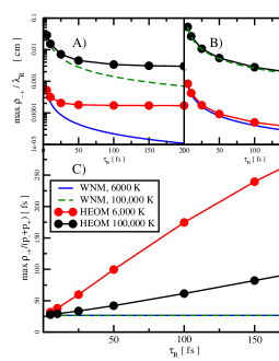
Figure 3: Comparison between the HEOM and WNM models in the weak radiation regime for gradually increasing coherence time of the sunlight at the radiation temperature of $T_{R}=6000\;\mathrm{K}$ or $T_{R}=100,000\;\mathrm{K}$. Fig. (a) shows the maximal amplitude of the steady state coherence $\rho_{-+}(t)$ extracted at long times with $\gamma_{R}=0.2$ fs^-1. Fig. (b) shows the dependence of the pumping rate $p_{+}$ on the coherence time of the radiation field, $\tau_{\mathrm{R}}$. The pumping rate $p_{2}$ is almost the same as $p_{-}$ and is not plotted. Fig. (c) shows the normalized coherence $\max\{\rho_{-+}(t)\}/{(p_{+}+p_{-})}$, which is independent of the radiation intensity for weak fields. The other parameters are given by $J=0$, $\epsilon_{1}=9900$ cm^-1 and $\epsilon_{2}=10000$ cm^-1.

As can be seen in the insert of Fig. 2, the difference between the HEOM and WNM models are the small transient dynamics upon excitation, resulting in a slight offset in the populations and a phase shift in the coherence. Otherwise, the overall agreement between the two models is excellent. Table 1 quantifies the pumping rates predicted by both models. In the weak field regime, the HEOM result should reproduce the Redfield rate.

Further, we study the dependence on the coherence time of the radiation, $\tau_{\mathrm{R}}=1/\gamma_{R}$. The agreement between HEOM and WNM deteriorates with the increase of the light coherence time, $\tau_{\rm R}$. To quantify this difference, we use two quantities that can easily be extracted from the exciton dynamics: The maximum of the oscillating coherence $\rho_{+-}$ (or $\rho_{-+}$), taken after the transient dynamics, and the pumping rates $p_{+}$ and $p_{-}$, defined as the derivatives of the linearly growing populations $\rho_{++}(t)$ and $\rho_{--}(t)$. We compare the two quantities for two radiation temperatures of $T_{R}=6000\;\mathrm{K}$ and $T_{R}=100,000\;\mathrm{K}$. The latter conveniently represents the classical limit at high temperatures. As can be seen in Fig. 3, all models match well at short coherence time, $\tau_{\mathrm{light}}=5\;\mathrm{fs}$, but with a gradual increase of the coherence time, the WNM model underestimates the amount of coherence present in the system, particularly for the temperature $6000\;\mathrm{K}$. While the WNM captures the pumping rates well, the predicted coherence term converges to zero instead of a constant for long coherence time $\tau_{\mathrm{light}}$.

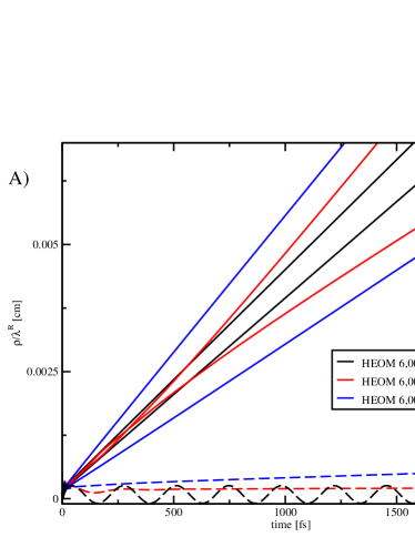
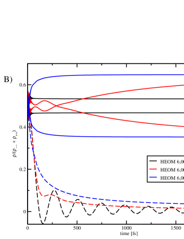
Figure 4: Dynamics of an open dimer system described in Results and Discussion section. Fig. (a) shows the population and the real part of the coherence for $\lambda=0$, $\lambda=10\;\mathrm{cm}^{-1}$ and $\lambda=150\;\mathrm{cm}^{-1}$ in black, red and blue lines. Fig. (b) shows the population and the coherence normalized by the sum of populations of single-excited states, i.e., the relative coherence within the manifold of single-excitedstates.

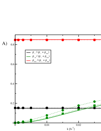
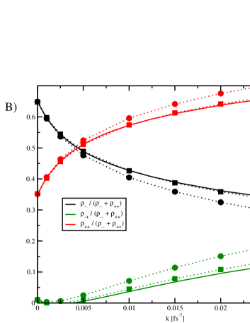
Figure 5: Dependence of the dimer system’s non-equilibrium steady-state on the decay rate $k$. The system parameters are $J=50\;\mathrm{cm}^{-1},\epsilon_{1}=9900\;\mathrm{cm}^{-1},\epsilon_{2}=10000\;\mathrm{cm}^{-1}$, and the effective temperature of the radiation field is $T_{R}=6000\;\mathrm{K}$. The HEOM results for $\gamma_{R}=0.1\;\mathrm{fs}^{-1}$ and $\gamma_{R}=1\;\mathrm{fs}^{-1}$ are shown with circle symbols and square symbols, respectively. The theoretical WNM result given by Eq. (11) is shown in full lines. Fig. (a) shows the results without coupling to a phonon bath. Fig. (b) shows the results with coupling to a phonon bath for which $\lambda_{1}=\lambda_{2}=100\;\mathrm{cm}^{-1},\gamma_{1}=\gamma_{2}=100\;\mathrm{fs}$ and temperature $T_{1}=T_{2}=300\;\mathrm{K}$. Changing $k$ scans the system dynamics: for fast $k$, the system approaches a pure state $\hat{\mu}|\bar{g}\rangle\langle\bar{g}|\hat{\mu}$; for slow $k$, the system steady-state is given by the phonon bath thermal state Eq. (12) without pumping, including the small amount of coherence due to bath redefinition of the basis. The steady states between these two extremes are closely related to the dynamics under no light pumping initiated with a $\delta$-pulse through Eq. (11).

III.2 Excitonic Coherence in Open Systems

The systems relevant in the primary processes of photosynthesis are open systems, so here we investigate the excitonic dynamics of open systems under pumping by incoherent light in the HEOM model. Unlike in the previous discussion of closed systems, the choice $J=0$ would be a special case and is no longer assumed; instead, $J=50$ cm^-1 is used. The radiation field has the temperature of $T_{R}=6000\;\mathrm{K}$ and a coherence time of $\tau_{\mathrm{light}}=10\;\mathrm{fs}$. The coupling to the electromagnetic field is assumed to be weak such that the density matrix can be normalized by the reorganization energy of the radiation field, $\lambda_{R}$. The dipole moments are parallel and have relative strengths of $\mu_{1}/\mu=0.60$ and $\mu_{2}/\mu=1.28$ in the local basis. The phonon baths are uncorrelated between the two sites, and have the same reorganization energy $\lambda=\lambda_{1}=\lambda_{2}$, temperature $T_{1}=T_{2}=300\;\mathrm{K}$, and cutoff frequency $\gamma_{1}=\gamma_{2}=100\;\mathrm{cm}^{-1}$. Fig. 4 gives the time evolution of the exciton populations and coherence for three values of the phonon bath reorganization energies, $\lambda=0$ (closed system), $\lambda=10\;\mathrm{cm}^{-1}$ and $\lambda=150\;\mathrm{cm}^{-1}$, respectively. For comparison, the same dynamics is normalized by the sum of excited state populations, which better demonstrates the relative coherence between the excited states.

We can make several observations about the exciton dynamics. For the closed system, the ratio of the populations is given solely by the couplings of the states to the electromagnetic field. In the presence of the phonon bath, this ratio is given by the coupling to the radiation at short times, which corresponds to the state $\hat{{\mu}}|\bar{g}\rangle\langle\bar{g}|\hat{{\mu}}$, and gradually approaches the reduced thermal equilibrium, i.e., the static coherence, which is determined by the coupling to the phonon bath, $\rho_{eq}=\lim_{t\rightarrow\infty}\rho(t)$. To understand the effect, we can again invoke the ensemble picture discussed in the previous section and the description of second-order interactions with the radiation field. There is always a portion of molecules that were excited only recently and their state is very close to the pure quantum state $\hat{{\mu}}|\bar{g}\rangle\langle\bar{g}|\hat{{\mu}}$ with population ratios given by their coupling to the radiation. Every molecule, however, reaches the thermal equilibrium state determined by the phonon bath after a certain time, and the portion of such molecules grows linearly, which explains the behavior of the trace-normalized excited state manifold (Fig. 4(b) in the short and long time limits. The decay time of the coherence depends weakly on the phonon bath reorganization energy. However, in comparison to the closed system, even weak coupling to the phonon bath damps the oscillations observed in the coherence and give rise to a continuously decaying non-oscillatory coherence. At long times, the coherence does not decay to zero, as in an isolated system, but approaches a constant plateau. The non-vanishing plateau value of the coherence arises from the entanglement with the phonon bath, and this static coherence cannot be captured by the WNM Moix2012 .

III.3 Steady-State Distribution with Population Decay

Whether one should describe a sample of continuously excited molecules as an ensemble composed of molecules undergoing coherent dynamics, or adopt the point of view of decoherence theory, where every individually-excited molecule loses coherence through its entanglement with the radiation and phonon baths, is still an open question. Here, we establish a relationship between the non-equilibrium steady-state of the exciton system in the presence of a decay rate $k$ and the dynamics initiated by a coherent short pulse, which is usually probed by ultrafast nonlinear spectroscopy experiments.

Following the ensemble description of the dephasing dynamics, Eq. (9), we can write the steady-state of the excited molecules as

$$\rho_{\mathrm{steady}}\approx\int_{0}^{\infty}d\tau\;e^{-k\tau}\mathcal{U}(\tau)\hat{{\mu}}|\bar{g}\rangle\langle\bar{g}|\hat{{\mu}}\;,$$ (11)

where $\mathcal{U}(t)$ is the radiation free evolution super-operator, representing the dissipative dynamics resulting from the coupling to the phonon bath alone. Eq. (11) is exact for the $\delta$-correlated sunlight for which $\gamma_{R}\to\infty$. In other words, for strongly incoherent light, we can decompose the long time steady-state of the system into an ensemble of molecules excited by a $\delta$-pulse at different times, weighted by the survival probability determined by the relaxation to the ground state. Whether or not such a decomposition is truly physical, Eq. (11) shows a direct relationship between ultrafast coherent dynamics and the steady-state under pumping by incoherent light. The decay ate $k$ is a natural timescale to be compared with the lifetime of electronic coherence. The coherent dynamics only manifests in the steady state if the timescale for the decay to the ground state is comparable to the lifetime of dynamic coherence.

To demonstrate this connection, we study the dependence of the steady-state on the decay rate $k$. Calculations are performed by the HEOM on a molecular dimer with parameters $J=50\;\mathrm{cm}^{-1}$, $\epsilon_{1}=9900\;\mathrm{cm}^{-1}$, $\epsilon_{2}=10000\;\mathrm{cm}^{-1}$, pumped by weak light with temperature $T=6000\;\mathrm{K}$ and $\gamma_{R}=0.1\;\mathrm{fs}^{-1}$. Two cases are studied: a closed system with no phonon bath and an open system with uncorrelated phonon baths. Fig. 5 shows the dependence of the system steady-state on the decay rate $k$. Here, the trace of the density matrix on the excited state manifold is normalized. For a closed system (Fig. 5(a), we observe a gradual transition from the pure state $\hat{{\mu}}|\bar{g}\rangle\langle\bar{g}|\hat{{\mu}}$ for fast $k$, which corresponds to a $\delta$-pulse excitation, to the diagonal part of $\hat{{\mu}}|\bar{g}\rangle\langle\bar{g}|\hat{{\mu}}$ for slow $k$. In the presence of a phonon bath (Fig. 5(b)), the same transition happens between the state $\hat{{\mu}}|\bar{g}\rangle\langle\bar{g}|\hat{{\mu}}$ for fast $k$ and the thermal equilibrium state of the system under no pumping

$$\rho_{\mathrm{eq}}=\lim\limits_{t\to\infty}\mathcal{U}(t)\hat{{\mu}}|\bar{g}\rangle\langle\bar{g}|\hat{{\mu}}$$ (12)

for slow $k$. The reduced equilibrium distribution of the system is not canonical because of the coupling to the phonon bath and can be obtained directly by stochastic path integral simulations or polaron transformation Moix2012 . The steady state dependence shown in Fig. 5(b) is more complicated in comparison with the closed system shown in Fig. 5(a). If we compare the steady-state dependence with the result given by Eq. (11) for perfectly white noise, there are detectable differences from the HEOM result with $\tau_{\mathrm{R}}=10\;\mathrm{fs}$, but these differences disappear for $\tau_{\mathrm{R}}=1\;\mathrm{fs}$.

Although it is difficult to tune the decay rate $k$ experimentally, there is a close connection between the dynamics initiated by a $\delta$-pulse and the dynamics induced by natural sunlight. Since the reduced density matrix contains all the information about the measurements performed on the system, the excitonic coherence can have an effect on the energy transfer only if the light-induced coherent dynamics affects the steady state through Eq. (11). For this reason, if the excitonic coherence probed by 2DES spectroscopy plays a significant role in energy transfer, it will be relevant only in situations, where the decoherence lifetime is sufficiently long compared to the decay rate in the system. Although the decoherence lifetime in photosynthetic systems can be as high as several picoseconds Mercer2009a ; Panitchayangkoon2011a , this time-scale may not exceed the decay lifetime to the reaction center, which is approximately 50 ps Sundstrom1986 ; Timpmann1991 ; Zhang1992 in many species of photosynthetic bacteria. For this reason, enhancement of the energy transfer by the dynamical coherence induced by sunlight may not be a dominant effect. In contrast, the spatial, static coherence due to quantum delocalization has a persistent effect on energy transfer efficiency (e.g. LH2) and robustness (e.g. FMO), and this effect is independent of light-induced coherence.

IV CONCLUSIONS

Our results demonstrate that the incoherent nature of sunlight excitation does not exclude transient coherence in the light-induced exciton dynamics but this dynamical coherence may not play a dominant role in light-harvesting energy transfer which is governed by static coherence resulting from the coupling to phonons.

• For a realistic light-harvesting system, the excitonic coherence is dynamical at short times, but becomes static at long times, which corresponds to the delocalization of states. The amount of dynamical coherence of a closed system is inversely proportional to the excitonic energy gap, and depends the coupling to the phonon bath.

• The decay to the ground state establishes a non-equilibrium steady state and defines an observation window for the induced exciton dynamics. Under the influence of the phonon bath, as the decay time increases, the steady state population distribution changes from photon-induced to phonon-induced, and the steady state coherence changes from dynamical to static. In the fast decay rate limit, the amount of steady coherence corresponds to the dynamical coherence and increases with the decay rate. whereas the slow-decay limit of the coherence is exactly the reduced equilibrium distribution.

• The contribution of the dynamical coherence to the system steady-state depends critically on the ratio of the lifetime of the dynamical coherence and the decay rate to the ground state. For photosynthetic light-harvesting systems, the light-induced dynamics lasts for hundreds of femtoseconds, whereas the observed energy trapping occurs on tens of picoseconds; therefore the light-induced coherence is dissipated on the trapping time-scale and is generally not a major factor consideration in efficiency light-harvesting energy transfer.

• Theoretically, the proposed white-noise model (WNM) with Redfield rates provides a reliable description of the excitation dynamics. As a result, the short coherence time of sunlight enables us to establish a simple connection between the dynamics excited by an ultra-short laser pulse as probed by 2DES spectroscopy and the steady-state of the excitonic system under pumping.

Appendix A Quantum description of the sunlight

To ensure generality of the results, we use a fully quantum description of the radiation. The radiation bath and system-bath interactions are in the Schrödinger picture defined as GreinerBook

$$\hat{H}_{R}= \;\sum_{\sigma\mathbf{k}}\hbar\omega_{\mathbf{k}}\left(\hat{b}_{\sigma\mathbf{k}}^{\dagger}\hat{b}_{\sigma\mathbf{k}}+\frac{1}{2}\right)\;,$$ (13)

$$\hat{H}_{S-R}= \;-\sum_{m\in\{x,y,z\}}\hat{E}_{m}{\otimes}\hat{{\mu}}_{m}\;.$$ (14)

They are expressed in terms of photon creation (annihilation) operators $\hat{b}_{\sigma\mathbf{k}}^{\dagger}~{}(\hat{b}_{\sigma\mathbf{k}})$ for different wave-vectors $\mathbf{k}$, polarizations $\sigma$ and frequencies $\omega_{\mathbf{k}}$. The interaction term in the dipole approximation couples the system and radiation field. The coupling to the system is through the $m$-th spatial component of the total dipole-moment operator $\hat{\mu}_{m}$. The radiation field part is described by

$$\hat{E}_{m}=i\sum_{\mathbf{k}}N_{\mathbf{k}}\boldsymbol{\varepsilon}^{\mathbf{k}m}\left(\hat{b}_{m\mathbf{k}}-\hat{b}_{m\mathbf{k}}^{\dagger}\right)\;.$$ (15)

The polarization vectors $\boldsymbol{\varepsilon}^{\mathbf{k}m}$ are orthogonal to $\mathbf{k}$ and to each other. The field is quantized in a box of a size $L$ and the limit $L\to\infty$ is to be performed at the end of our calculations GreinerBook . In SI units, this corresponds to normalization constants

$$N_{\mathbf{k}}=\sqrt{\frac{\hbar\omega_{\mathbf{k}}}{2L^{3}\epsilon_{0}}}\;,$$ (16)

where $\epsilon_{0}$ denotes the vacuum permittivity.

In order to express the equations in an unified way, we rewrite Eq. (14) as

$$\hat{H}_{S-R}=\sum_{m\in\{x,y,z\}}\hat{V}_{R_{m}}{\otimes}\hat{K}_{R_{m}}$$ (17)

where $\hat{K}_{R_{m}}=\hat{\mu}_{m}/\mu_{m}$ and $\hat{V}_{R_{m}}=-\mu_{m}\hat{E}_{m}$. The constant $\mu_{m}=\frac{1}{2}\sqrt{\mathrm{Tr}\,\hat{\mu}_{m}\cdot\hat{\mu}_{m}}$ denotes the magnitude of the $m$-th component of the dipole moment. The information about the electric field strength and the magnitude of the dipole moment is kept in the bath operators $\hat{V}_{R_{m}}$ and enters through the radiation reorganization energy $\lambda_{R}$, while the system operators $\hat{K}_{R_{m}}$ hold the dimensionless matrix structure of the dipole moments. In order to lower the computational cost, we choose both molecules to have parallel dipole moments, which allows us to use only one bath ($\hat{K}_{R},\hat{V}_{R}$) and avoid the orientational averaging. However, the essential physics will not be changed. We drop the coordinate index $m$ for the total dipole moment operator $\hat{\mu}$ and we assume that it is taken along the axis of the dipole moment. In the manuscript, we use quantities $\mu$ and $\hat{E}$ instead of $\mu_{m}$ and $\hat{E}_{m}$.

Appendix B Hierarchical Equations of Motion

In order to describe the solar light and phonon baths quantum mechanically, we use the Hierarchical Equations of Motion as Tanimura1989a

$$\dot{\hat{\rho}}^{n_{\alpha k}}(t) =-\left(i\hat{H}_{S}^{\times}+\sum_{\alpha}\sum_{k=0}^{M}n_{\alpha k}\nu_{\alpha k}\right)\hat{\rho}^{n_{\alpha k}}(t)$$

$$-\sum_{\alpha}\left(\frac{2\lambda_{\alpha}}{\beta_{\alpha}\gamma_{\alpha}}-i\lambda_{\alpha}-\sum_{k=0}^{M}\frac{c_{\alpha k}}{\nu_{\alpha k}}\right)\hat{K}_{\alpha}^{\times}\hat{K}_{\alpha}^{\times}\hat{\rho}^{n_{\alpha k}}(t)$$

$$-i\sum_{\alpha}\sum_{k=0}^{M}\hat{K}_{\alpha}^{\times}\hat{\rho}^{n_{\alpha k}^{+}}(t)$$

$$-i\sum_{\alpha}\sum_{k=0}^{M}n_{\alpha k}\left(c_{\alpha k}\hat{K}_{\alpha}\hat{\rho}^{n_{\alpha k}^{-}}(t)-c_{\alpha k}^{*}\hat{\rho}^{n_{\alpha k}^{-}}(t)\hat{K}_{\alpha}\right)$$ (18)

written in the standard notation Dijkstra2010 . HEOM introduces an infinite set of operators $\hat{\rho}^{n_{\alpha k}}(t)$ numbered by a multi-index $n_{\alpha k}$ to represent entanglement with the bath and the bath memory effects. The index $\alpha\in\{R,1,2\}$ denotes all baths present, both radiation and phonon ones, while the index $k$ denotes the Matsubara frequencies $\nu_{\alpha k}=2\pi k/\beta_{\alpha}$ included up to some maximum frequency $M$. For convenience, we define $\nu_{\alpha 0}=\gamma_{\alpha}$. The standard definition of inverse temperature $\beta_{\alpha}=1/k_{B}/T_{\alpha}$ is used. Each of the integer numbers $n_{\alpha k}$ can attain values from 0 to infinity, but in praxis they are truncated after a sufficient number of tiers $\Theta_{\mathrm{max}}$. Only operators $\hat{\rho}^{n_{\alpha k}}(t)$ for which $\sum_{\alpha}\sum_{k=0}^{M}n_{\alpha k}\leq\Theta_{\mathrm{max}}$ are taken into account. We use abbreviations $n_{\alpha k}^{+}=n_{\alpha k}+1$, $n_{\alpha k}^{-}=n_{\alpha k}-1$,

$$c_{\alpha k} =\frac{4\lambda_{\alpha}\gamma_{k}}{\beta_{\alpha}}\frac{\nu_{\alpha k}}{\nu_{\alpha k}^{2}-\gamma_{\alpha}^{2}}\;,$$ (19)

$$c_{\alpha 0} =\lambda_{\alpha}\gamma_{\alpha}(\cot(\beta_{\alpha}\gamma_{\alpha}\hbar/2)-i)$$ (20)

to make the notation more compact. The physical density matrix is the operator $\hat{\rho}^{n_{\alpha k}}(t)$ for which all $n_{\alpha k}=0$. The symbol $\hat{A}^{\times}$ denotes Liouville space operator (superoperator) defined by its action on a (Hilbert space) operator $\bullet$ as $\hat{A}^{\times}\bullet=[\hat{A},\bullet]$ for a given operator $\hat{A}$.

The equations (18) assume a Drude-Lorentz bath with EGCF in a form

$$C^{\alpha}(t)= \hbar c_{\alpha 0}\exp(-\gamma_{\alpha}t)+\sum_{k=1}^{\infty}c_{\alpha k}\exp\left(-\nu_{\alpha k}t\right)\;,$$ (21)

where $\alpha\in\{R,1,2\}$.

The computational cost of the full form of the equations (18) is extremely high, especially at low temperature. To deal with this difficulty, a hybrid version, i.e., the stochastic-HEOM, has been developed to simulate low-temperature dynamics, and various high-temperature approximations have been successfully used Ishizaki2009a ; Kreisbeck2011a ; Moix2013 , effectively reducing the number of included Matsubara frequencies to zero ($M=0$) or approximating the first Matsubara frequency without further computational costs Ishizaki2009a . These approximations need two conditions to be met: $\beta\hbar\gamma\ll 1$ and $\beta\Delta\ll 1$, where $\Delta$ is a characteristic energy gap of the system. In order to describe incoherent natural light, we use a bath with a temperature $T_{R}=6000\;\mathrm{K}$, coherence time $\gamma_{R}\approx 0.1\;\mathrm{fs}^{-1}$ and $\Delta=10,000\;\mathrm{cm}^{-1}$, which gives us $\beta_{R}\hbar\gamma_{R}\approx 0.13$ and $\beta_{R}\Delta\approx 2.40$. While the first criterion is well satisfied in our calculation, the second leads to incorrect results and Matsubara frequencies up to the second one need to be included.

In part of presented calculations, we use HEOM (18) together with a decay rate $k$ from the excited state manifold to the ground state. Is such a case, the rate is applied to all operators $\hat{\rho}^{n_{\alpha k}}(t)$ from Eq. (18)

$$\langle\bar{e}_{u}|\dot{\hat{\rho}}^{n_{\alpha k}}(t)|\bar{e}_{v}\rangle= \;\langle\bar{e}_{u}|\dot{\hat{\rho}}_{\mathrm{HEOM}}^{n_{\alpha k}}(t)-k\hat{\rho}^{n_{\alpha k}}(t)|\bar{e}_{v}\rangle\;,$$ (22a)

$$\langle g|\dot{\hat{\rho}}^{n_{\alpha k}}(t)|g\rangle= \;\langle g|\dot{\hat{\rho}}_{\mathrm{HEOM}}^{n_{\alpha k}}(t)|g\rangle$$

$$+k\sum_{u}\langle\bar{e}_{u}|\hat{\rho}^{n_{\alpha k}}(t)|\bar{e}_{u}\rangle\;.$$ (22b)

Here, $\dot{\hat{\rho}}_{\mathrm{HEOM}}^{n_{\alpha k}}(t)$ denotes the reduced density matrix derivative calculated from the Eq. (18). We refer to this set of equations as the HEOM with rate.

Appendix C Stochastic wavefunction solution: White noise model

In this paper, a ground state and two single-excited states of a molecular dimer are modeled as a three-level system, given by

$$~{}\hat{H}_{S}=\sum_{v=1,2}\epsilon_{v}|\bar{e}_{v}{\rangle}{\langle}\bar{e}_{v}|+\epsilon_{g}|\bar{g}{\rangle}{\langle}\bar{g}|+J(|\bar{e}_{1}{\rangle}{\langle}\bar{e}_{2}|+H.c.),$$

where $\epsilon_{v}~{}(v=1,2,g)$ is the site energy of the exciton for the local state $|\bar{e}_{v}{\rangle}$ and the ground state $|\bar{g}{\rangle}$, and $J$ is the resonance coupling between states $|\bar{e}_{1}{\rangle}$ and $|\bar{e}_{2}{\rangle}$. Without loss of generality, we set the ground state energy $\epsilon_{g}=0$ as the energy reference.

Under excitation by natural sunlight, the system interacts with the radiation field via the dipole coupling as

$$~{}\hat{H}_{S-R}=\hat{V}_{R}{\otimes}\hat{K}_{R}=-\hat{E}{\otimes}\sum_{v=1,2}[\mu_{v}|\bar{e}_{v}{\rangle}{\langle}\bar{g}|+H.c.],$$ (24)

where the exciton dipole moment is described as $\hat{K}_{R}=\sum_{v=1,2}(\frac{\mu_{v}}{\mu}|\bar{e}_{v}{\rangle}{\langle}\bar{g}|+H.c.)$, with the magnitude of the collective dipole moment defined as $\mu=\sqrt{\mu^{2}_{1}+\mu^{2}_{2}}$. The re-weighted radiation field is given by $\hat{V}_{R}=-\mu\hat{E}$, where $\hat{E}$ is the photon field. Practically, the radiation field can be characterized by the so-called energy gap correlation function $C_{R}(t)={\langle}\hat{V}_{R}(t)\hat{V}_{R}(0){\rangle}$, where the time-dependence in $\hat{V}_{R}(t)$ denotes the interaction picture. Moreover, we also include the decay processes from the excited state to the ground state in this study. This represents e.g. the exciton trapping by the reaction-center in the light-harvesting complexes.

If the exciton-photon dipole coupling is sufficiently weak and the temperature of the radiation field is high, we can represent the radiation field stochastically. Then, the dipole interaction simplifies to $\hat{H}_{S-R}=\xi\hat{K}_{R}$, where $\xi$ is the stochastic field. If we define the wavefunction of the exciton as $|\psi(t){\rangle}=C_{1}(t)|\bar{e}_{1}{\rangle}+C_{2}(t)|\bar{e}_{2}{\rangle}+C_{g}(t)|\bar{g}{\rangle}$, the equation of motion under the stochastic field can be shown to be

$$~{}\frac{dC_{1}(t)}{dt} = -i\frac{J}{\hbar}C_{2}(t)-(i\frac{\epsilon_{1}}{\hbar}+\frac{\kappa}{2})C_{1}(t)-i\xi_{1}C_{g}(t)$$

$$\frac{dC_{2}(t)}{dt} = -i\frac{J}{\hbar}C_{1}(t)-(i\frac{\epsilon_{2}}{\hbar}+\frac{\kappa}{2})C_{2}(t)-i\xi_{2}C_{g}(t),$$

with the radiation field $\xi_{v}=\frac{\mu_{v}}{\mu}\xi$, and the decay rate $\kappa$. In the weak-field limit $C_{g}(t){\approx}1$, the Eq. (C) reduces to

$$~{}\frac{dC_{1}(t)}{dt} = -i\frac{J}{\hbar}C_{2}(t)-(i\frac{\epsilon_{1}}{\hbar}+\frac{\kappa}{2})C_{1}(t)-i\xi_{1}$$ (26)

$$\frac{dC_{2}(t)}{dt} = -i\frac{J}{\hbar}C_{1}(t)-(i\frac{\epsilon_{2}}{\hbar}+\frac{\kappa}{2})C_{2}(t)-i\xi_{2}.$$

By using the Laplace transformation, the wavefunction coefficients and the radiation field are changed to $C_{v}(z)=\int^{\infty}_{0}e^{-zt}C_{v}(t)dt$ and $\xi_{v}(z)=\int^{\infty}_{0}e^{-zt}\xi_{v}(t)dt$, respectively. The equation of motion in the Laplace picture is described as

$$~{}\begin{pmatrix}z+\frac{\kappa}{2}+i\frac{\epsilon_{1}}{\hbar}&i\frac{J}{\hbar}\\ i\frac{J}{\hbar}&z+\frac{\kappa}{2}+i\frac{\epsilon_{2}}{\hbar}\\ \end{pmatrix}\begin{pmatrix}C_{1}(z)\\ C_{2}(z)\\ \end{pmatrix}=-i\begin{pmatrix}\xi_{1}(z)\\ \xi_{2}(z)\\ \end{pmatrix}.$$

The Hamiltonian $\hat{H}_{S}$ can be diagonalized by transformation into the excitonic basis. Through the transfer matrix $\hat{S}$, it is obtained by $\hat{S}\hat{H}_{S}\hat{S}^{{\dagger}}=\sum_{v=\pm}\epsilon_{v}|\bar{e}_{v}{\rangle}{\langle}\bar{e}_{v}|$, with $\epsilon_{\pm}$ the eigen-energy, and $|\bar{e}_{\pm}{\rangle}$ the corresponding excitonic states. Then, the equation of motion at Eq. (C) is transformed to

$$~{}\begin{pmatrix}z+\frac{\kappa}{2}+i\frac{\epsilon_{+}}{\hbar}&0\\ 0&z+\frac{\kappa}{2}+i\frac{\epsilon_{-}}{\hbar}\\ \end{pmatrix}\begin{pmatrix}{C}_{+}(z)\\ {C}_{-}(z)\\ \end{pmatrix}=-i\begin{pmatrix}{\xi}_{+}(z)\\ {\xi}_{-}(z)\\ \end{pmatrix}$$

where the coefficients and the radiation field between the local basis and the excitonic basis are connected by $[{C}_{+}(z),{C}_{-}(z)]^{T}=\hat{S}[C_{1}(z),C_{2}(z)]^{T}$ and $[{\xi}_{+}(z),{\xi}_{-}(z)]^{T}=\hat{S}[\xi_{1}(z),\xi_{2}(z)]^{T}$, respectively. As a result, the expression of the time dependent coefficients at Eq. (C) in the excitonic basis are given by

$${C}_{+}(t) = -i\int^{t}_{0}e^{-(\frac{\kappa}{2}+i{\epsilon_{+}}/{\hbar})(t-\tau)}{\xi}_{+}(\tau)d{\tau},$$ (29)

$${C}_{-}(t) = -i\int^{t}_{0}e^{-(\frac{\kappa}{2}+i{\epsilon_{-}}/{\hbar})(t-\tau)}{\xi}_{-}(\tau)d{\tau},$$

with ${\xi}_{v}(\tau)=\frac{{\mu}_{v}}{\mu}V_{R}(\tau)~{}(v=\pm)$, which can be characterized by the correlation function as ${\langle}{\xi}_{v}(t){\xi}_{v^{\prime}}(0){\rangle}=\frac{{\mu}_{v}{\mu}_{v^{\prime}}}{\mu^{2}}C_{R}(t)$. Hence, the population $\rho_{vv}(t)={\langle}{C}^{*}_{v}(t){C}_{v}(t){\rangle}$ at the eigen-state $|\bar{e}_{v}{\rangle}~{}(v=\pm)$ is expressed as

$$~{}\rho_{vv}(t) = \int^{t}_{0}d{\tau_{1}}e^{-(\frac{\kappa}{2}-i\epsilon_{v}/\hbar)(t-\tau_{1})}$$

$${\times}\int^{t}_{0}d{\tau_{2}}e^{-(\frac{\kappa}{2}+i\epsilon_{v}/\hbar)(t-\tau_{2})}{\langle}{\xi}_{v}(\tau_{1}){\xi}_{v}(\tau_{2}){\rangle}.$$

The coherence $\rho_{+-}(t)={\langle}{C}^{*}_{-}(t){C}_{+}(t){\rangle}$ is given by

$$~{}\rho_{+-}(t) = \int^{t}_{0}d{\tau_{1}}e^{-(\frac{\kappa}{2}-i\epsilon_{-}/\hbar)(t-\tau_{1})}$$

$${\times}\int^{t}_{0}d{\tau_{2}}e^{-(\frac{\kappa}{2}+i\epsilon_{+}/\hbar)(t-\tau_{2})}{\langle}{\xi}_{-}(\tau_{1}){\xi}_{+}(\tau_{2}){\rangle}.$$

It should be noted that this is the general solution, which does not rely on the detailed information of correlation function for the radiation field. The only prerequisite condition is the weak-field limit. In the following, we consider the $\delta$-function noise, which is the simplest case of the radiation field.

C.1 $\delta$-function noise

If the coherence time of the radiation field is sufficitently short, the field can be considered to be Gaussian, with the corresponding correlation function specified by $C_{R}(t)=I^{R}\delta(t)$, as shown in Eq. (6). Such model is often called white noise model, or the Haken-Strobl model in the weak field limit. Straightforwardly, the populations at states $|\bar{e}_{+}{\rangle}$ and $|\bar{e}_{-}{\rangle}$ are given by

$$~{}\rho_{++}(t)=\frac{{\mu}^{2}_{+}I^{R}_{+}}{\mu^{2}\kappa}(1-e^{-\kappa{t}}),$$ (32)

$$\rho_{--}(t)=\frac{{\mu}^{2}_{-}I^{R}_{-}}{\mu^{2}\kappa}(1-e^{-\kappa{t}}),$$ (33)

with the radiation field pumping rates $I^{R}_{+}=I^{R}$ and $I^{R}_{-}=I^{R}$. The coherence term is given by

$$~{}\rho_{+-}(t)=\frac{{\mu}_{+}{\mu}_{-}(I^{R}_{+}+I^{R}_{-})/2}{\mu^{2}(\kappa+i\epsilon/\hbar)}(1-e^{-(\kappa+i\epsilon/\hbar)t}),$$ (34)

with $\epsilon=\epsilon_{+}-\epsilon_{-}$. From the results for the populations and the coherence, it is found that the functional expression of them will keep the same, which implies that the physical picture is unchanged for arbitrary inter-site coupling $J$.

In absence of the decay process ($\kappa{\rightarrow}0$), the excitation is accumulated under the incoherent photon pumping. As a result, the populations exhibit linear increase of the time. On the other hand, the coherence shows Rabi oscillations with finite amplitude due to the existence of the energy gap. Hence, after a long time evolution (still in the weak-field limit), the coherence becomes negligible compared to the populations. However, if the decay process is tuned on, both the population and coherence terms will approach the steady state, and the static coherence occurs naturally.

C.2 Pumping rates from quantized radiation field

The above analysis of the dynamics for the three level molecular dimer system is based on the classical white noise, which is also known as the Haken-Strobl-Reineker Model. The classical radiation field can be connected with the theory with general quantum light by evaluating the Redfield pumping rates. Specifically, we write the exciton-photon interaction Hamiltonian $\hat{H}_{S-R}$, Eqs. (II.1,14), in the interaction picture and the excitonic basis as

$$~{}\hat{H}_{S-R}(t) = [\frac{{\mu}_{+}}{\mu}e^{i\epsilon_{+}t/\hbar}|\bar{e}_{+}{\rangle}{\langle}\bar{g}|+\frac{{\mu}_{-}}{\mu}e^{i\epsilon_{-}t/\hbar}|\bar{e}_{-}{\rangle}{\langle}\bar{g}|+H.c.]$$ (35)

$${\otimes}\hat{V}_{R}(t).$$

We rewrite the radiation field quantization, Eq. (15), with use of operators $V_{R}$ as $\hat{V}_{R}(t)=\sum_{k}(g_{k}e^{i\omega_{k}t}\hat{b}^{{\dagger}}_{k}+g^{*}_{k}e^{-i\omega_{k}t}\hat{b}_{k})$, with $\hat{b}^{{\dagger}}_{k}(\hat{b}_{k})$ creation(annihilation) one photon having frequency $\omega_{k}$ in the momentum $k$. The coupling constants $g_{k}$ are given by relation $g_{k}=i\mu N_{k}\boldsymbol{\varepsilon}^{k}$, where $\boldsymbol{\varepsilon}^{k}$ denotes projection of $\boldsymbol{\varepsilon}^{\mathbf{k}m}$ in the direction of molecular dipole moment, and $N_{k}$ is the normalization constant given at Eq. (A4). In this paper, the radiation field is specified as the Drude-Lorentz spectrum $J(\omega)=\pi\sum_{k}|g_{k}|^{2}\delta(\omega-\omega_{k})={2\hbar\lambda_{R}\gamma_{R}\omega}/{(\gamma^{2}_{R}+\omega^{2})}$, with $\lambda_{R}$ the coupling strength and $\gamma_{R}$ the cutoff frequency. Hence, based on the second order perturbation, the pumping rate of the first excited state is obtained by

$$~{}I^{R}_{+} = \int^{\infty}_{-\infty}d{\tau}\sum_{k}|g_{k}|^{2}n_{k}e^{i(\omega_{k}-\epsilon_{+}/\hbar)\tau}$$ (36)

$$= \frac{2\lambda_{R}\gamma_{R}\epsilon_{+}(\coth(\beta_{R}\epsilon_{+}/2)-1)}{\gamma^{2}_{R}+(\epsilon_{+}/\hbar)^{2}},$$

with the Bose-Einstein distribution $n_{k}=1/[\exp(\beta_{R}\hbar\omega_{k})-1]$ and $\beta_{R}=1/(k_{b}T_{R})$. Similarly, the pumping rate for the second excited state is obtained by

$$~{}I^{R}_{-}=\frac{2\lambda_{R}\gamma_{R}\epsilon_{-}(\coth(\beta_{R}\epsilon_{-}/2)-1)}{\gamma^{2}_{R}+(\epsilon_{-}/\hbar)^{2}}.$$ (37)

Moreover, the corresponding stimulating emission rate for the relaxation process is given by $I^{\textrm{em}}_{v}={2\lambda_{R}\gamma_{R}\epsilon_{v}(\coth(\beta_{R}\epsilon_{v}/2)+1)}/{(\gamma^{2}_{R}+(\epsilon_{v}/\hbar)^{2})}$. It is found that the pumping rate and emission rate obey the detailed balance relation as $I^{R}_{v}/I^{\textrm{em}}_{v}=\exp(-\beta_{R}\epsilon_{v})$.

While for the pump rate of the coherence term $\rho_{+-}$, the expression is given by

$$~{}I^{R}_{+-} = \int^{\infty}_{0}d{\tau}\sum_{k}|g_{k}|^{2}n_{k}[e^{i(\omega_{k}-\epsilon_{+}/\hbar)\tau}+e^{-i(\omega_{k}-\epsilon_{-}/\hbar)\tau}]$$ (38)

$$= (I^{R}_{+}+I^{R}_{-})/2.$$

References

- (1) G. S. Engel, T. R. Calhoun, E. L. Read, T. K. Ahn, T. Mančal, Y. C. Cheng, R. E. Blankenship, and G. R. Fleming, Nature (London) 446, 782 (2007).
- (2) I. P. Mercer, Y. C. El-Taha, N. Kajumba, J. P. Marangos, J. W. G. Tisch, M. Gabrielsen, R. J. Cogdell, E. Springate, and E. Turcu, Phys. Rev. Lett. 102, 057402 (2009).
- (3) E. Collini, C. Y. Wong, K. E. Wilk, P. M. G. Curmi, P. Brumer, and G. D. Scholes, Nature (London) 463, 644 (2010).
- (4) X. P. Jiang and P. Brumer, J. Chem. Phys. 94, 5833 (1991).
- (5) T. Mančal and L. Valkunas, New J. Phys. 12, 065044 (2010).
- (6) Y. Tanimura and R. Kubo, J. Phys. Soc. Jpn. 58, 101 (1989).
- (7) A. Ishizaki and G. R. Fleming, Proc. Natl. Acad. Sci U.S.A. 106, 17255 (2009).
- (8) A. G. Dijkstra and Y. Tanimura, Phys. Rev. Lett. 104, 250401 (2010).
- (9) J. M. Moix and J. Cao, J. Chem. Phys. 139, 134106 (2013).
- (10) M. Shapiro, Phys. Rev. Lett. 110, 153003 (2013).
- (11) J. Cao, J. Phys. Chem. B 110, 19040 (2006).
- (12) S. Mukamel, Principles of Nonlinear Spectroscopy (Oxford University Press, Oxford, 1995).
- (13) V. May and O. Kühn, Charge and Energy Transfer Dynamics in Molecular Systems (Wiley-VCH, Berlin, 2001).
- (14) J. Olšina and T. Mančal, J. Mol. Model. 16, 1765 (2010).
- (15) H. Haken and G. Strobl, Zeitschrift für Physik 262, 135 (1973).
- (16) J. Cao and R. J. Silbey, J. Phys. Chem. A 113 13825 (2009).
- (17) J. Wu, R. J. Silbey, and J. Cao, Phys. Rev. Lett. 110, 200402 (2013).
- (18) P. Brumer and M. Shapiro, Proc. Natl. Acad. Sci. U.S.A. 109, 19575 (2012).
- (19) T. V. Tscherbul and P. Brumer, Phys. Rev. Lett. accepted (2014). [A similar model was developed independently by the Brumer group]
- (20) J. M. Moix, Y. Zhao, and J. Cao, Phys. Rev. B 85, 115412 (2012).
- (21) G. Panitchayangkoon, D. V. Voronine, A. Darius, J. R. Caram, N. H. C. Lewis, S. Mukamel, and G. S. Engel, Proc. Natl. Acad. Sci. U.S.A 108, 20908 (2011).
- (22) V. Sundström, R. van Grondelle, H. Bergström, E. Akesson, and T. Gillbro, Biochimica et Biophysica Acta 851, 431 (1986).
- (23) K. Timpmann and A. Freiberg, Chem. Phys. Lett. 182, 617 (1991).
- (24) F. G. Zhang, T. Gillbro, R. van Grondelle, V. Sundström, Biophys. J. 61, 694 (1992).
- (25) C. Kreisbeck, T. Kramer, M. Rodriguez, and B. Hein, J. Chem. Theory comput. 7, 2166 (2011).
- (26) Greiner W (1998) Quantum Mechanics: Special Chapters (Springer-Verlag, Berlin Heidelberg New York).