Flower Pollination Algorithm: A Novel Approach for Multiobjective Optimization

Abstract

Multiobjective design optimization problems require multiobjective optimization techniques to solve, and it is often very challenging to obtain high-quality Pareto fronts accurately. In this paper, the recently developed flower pollination algorithm (FPA) is extended to solve multiobjective optimization problems. The proposed method is used to solve a set of multobjective test functions and two bi-objective design benchmarks, and a comparison of the proposed algorithm with other algorithms has been made, which shows that FPA is efficient with a good convergence rate. Finally, the importance for further parametric studies and theoretical analysis are highlighted and discussed.

Citation Details: X. S. Yang, M. Karamanoglu, X. S. He, Flower Pollination Algorithm: A Novel Approach for Multiobjective Optimization， Engineering Optimization, vol. 46, Issue 9, pp. 1222-1237 (2014).

1 Introduction

Real-world design problems in engineering and industry are usually multiobjective or multicriteria, and these multiple objectives are often conflicting one another, which makes it impossible to use any single design option without compromise. Common approaches are to provide good approximations to the true Pareto fronts of the problem of interest so that decision-makers can rank different options, depending on their preferences or their utilities (Abbass and Sarker 2002; Babu and Gujarathi 2007; Cagnina et al. 2008; Deb, 1999, 2000, 2001; Reyes-Sierra and Coello 2006). Compared with single objective optimization, multiobjective optimization has its additional challenging issues such as time complexity, inhomogeneity and dimensionality. It is usually more time consuming to obtain the true Pareto fronts because it usually requires to produce many points on the Pareto front for good approximations.

In addition, even accurate solutions on a Pareto front can be obtained, there is still no guarantee that these solution points will distribute uniformly on the front. In fact, it is often difficult to obtain the whole front without any part missing. For single objective optimization, the optimal solution can often be a single point in the solution space, while for bi-objective optimization, the Pareto front forms a curve, and for tri-objective cases, it becomes a surface. In fact, higher dimensional problems can have extremely complex hypersurface as its Pareto front (Madavan 2002; Marler and Arora 2004; Yang 2010a; Yang and Gandomi 2012). Consequently, it is typically more challenging to solve such high-dimensional problems.

In the current literature of engineering optimization, a class of nature-inspired algorithms have shown their promising performance and have thus become popular and widely used, and these algorithms are mostly swarm intelligence based (Coello 1999; Deb et al. 2002; Geem et al. 2001; Geem 2009; Ray and Liew 2002; Yang 2010,2010b,2011a; Gandomi and Yang 2011; Gandomi et al. 2012). Metaheuristic algorithms such as particle swarm optimization, harmony search and cuckoo search are among the most popular (Geem 2009; Yang 2010). For example, harmony search, developed by Zong Woo Geem in 2001 (Geem et al. 2001; Geem 2006, 2009), has been applied in many areas such as highly challenging water distribution networks (Geem 2006) and discrete structural optimization (Lee et al. 2005). Other algorithms such as shuffled frog-leaping algorithm and particle swarm optimizers have been applied to various optimization problems (Eusuff et al. 2006; He et al. 2004; Huang 1996). There are many reasons for the popularity of metaheuristic algorithms, and flexibility and simplicity of these algorithms certainly contribute to their success.

The main aim of this paper is to extend the flower pollination algorithm (FPA), developed by Xin-She Yang in 2012 (Yang 2012), for single objective optimization to solve multiobjective optimization, and thus developed a multi-objective flower pollination algorithm (MOFPA). The rest of this paper is organized as follows: Section 2 outlines the basic characteristics of flower pollination in nature and then introduce in detail the ideas of flower pollination algorithm. Section 3 then presents the validation of the FPA by numerical experiments and a few selected multiobjective benchmarks. Then, in Section 4, two real-world design benchmarks are solved to design a welded beam and a disc brake, each with two objectives. Finally, some relevant issues are discussed and conclusions are drawn in Section 5.

2 Flower Pollination Algorithm

2.1 Characteristics of Flower Pollination

It is estimated that there are over a quarter of a million types of flowering plants in Nature and that about 80% of all plant species are flowering species. It still remains a mystery how flowering plants came to dominate the landscape from the Cretaceous period (Walker 2009). Flowering plants have been evolving for at least more than 125 million years and flowers have become so influential in evolution, it is unimaginable what the plant world would look like without flowers. The main purpose of a flower is ultimately reproduction via pollination. Flower pollination is typically associated with the transfer of pollen, and such transfer is often linked with pollinators such as insects, birds, bats and other animals. In fact, some flowers and insects have co-evolved into a very specialized flower-pollinator partnership. For example, some flowers can only attract and can only depend on a specific species of insects or birds for successful pollination.

Pollination can take two major forms: abiotic and biotic. About 90% of flowering plants belong to biotic pollination. That is, pollen is transferred by pollinators such as insects and animals. About 10% of pollination takes abiotic form which does not require any pollinators. Wind and diffusion help pollination of such flowering plants, and grass is a good example of abiotic pollination (ScienceDaily 2001; Glover 2007). Pollinators, or sometimes called pollen vectors, can be very diverse. It is estimated there are at least about 200,000 varieties of pollinators such as insects, bats and birds. Honeybees are a good example of pollinators, and they have also developed the so-called flower constancy. That is, these pollinators tend to visit exclusive certain flower species while bypassing other flower species. Such flower constancy may have evolutionary advantages because this will maximize the transfer of flower pollen to the same or conspecific plants, and thus maximizing the reproduction of the same flower species. Such flower constancy may be advantageous for pollinators as well, because they can be sure that nectar supply is available with their limited memory and minimum cost of learning, switching or exploring. Rather than focusing on some unpredictable but potentially more rewarding new flower species, flower constancy may require minimum investment cost and more likely guaranteed intake of nectar (Waser 1986).

Pollination can be achieved by self-pollination or cross-pollination. Cross-pollination, or allogamy, means pollination can occur from pollen of a flower of a different plant, while self-pollination is the fertilization of one flower, such as peach flowers, from pollen of the same flower or different flowers of the same plant, which often occurs when there is no reliable pollinator available. Biotic, cross-pollination may occur at long distance, and the pollinators such as bees, bats, birds and flies can fly a long distance, thus they can considered as the global pollination. In addition, bees and birds may behave as Lévy flight behaviour with jump or fly distance steps obeying a Lévy distribution (Pavlyukevich 2007). Furthermore, flower constancy can be considered as an increment step using the similarity or difference of two flowers.

From the biological evolution point of view, the objective of the flower pollination is the survival of the fittest and the optimal reproduction of plants in terms of numbers as well as the most fittest. This can be considered as an optimization process of plant species. All the above factors and processes of flower pollination interact so as to achieve optimal reproduction of the flowering plants. Therefore, this may motivate us to design new optimization algorithms.

2.2 Flower Pollination Algorithm

Flower pollination algorithm (FPA) was developed by Xin-She Yang in 2012 (Yang 2012), inspired by the flow pollination process of flowering plants. FPA has been extended to multi-objective optimization (Yang et al. 2013). For simplicity, the following four rules are used:

1. Biotic and cross-pollination can be considered as a process of global pollination, and pollen-carrying pollinators move in a way which obeys Lévy flights (Rule 1).

2. For local pollination, abiotic pollination and self-pollination are used (Rule 2).

3. Pollinators such as insects can develop flower constancy, which is equivalent to a reproduction probability that is proportional to the similarity of two flowers involved (Rule 3).

4. The interaction or switching of local pollination and global pollination can be controlled by a switch probability $p\in[0,1]$, slightly biased towards local pollination (Rule 4).

In order to formulate the updating formulas, the above rules have to be converted into proper updating equations. For example, in the global pollination step, flower pollen gametes are carried by pollinators such as insects, and pollen can travel over a long distance because insects can often fly and move in a much longer range. Therefore, Rule 1 and flower constancy (Rule 3) can be represented mathematically as

$$\mbox{\boldmath$x$}_{i}^{t+1}=\mbox{\boldmath$x$}_{i}^{t}+\gamma L(\lambda)(\mbox{\boldmath$g$}_{*}-\mbox{\boldmath$x$}_{i}^{t}),$$ (1)

where $\mbox{\boldmath$x$}_{i}^{t}$ is the pollen $i$ or solution vector $\mbox{\boldmath$x$}_{i}$ at iteration $t$, and $\mbox{\boldmath$g$}_{*}$ is the current best solution found among all solutions at the current generation/iteration. Here $\gamma$ is a scaling factor to control the step size.

Here $L(\lambda)$ is the parameter, more specifically the Lévy-flights-based step size, that corresponds to the strength of the pollination. Since insects may move over a long distance with various distance steps, a Lévy flight can be used to mimic this characteristic efficiently. That is, $L>0$ is drawn from a Lévy distribution

$$L\sim\frac{\lambda\Gamma(\lambda)\sin(\pi\lambda/2)}{\pi}\frac{1}{s^{1+\lambda}},\quad(s\gg s_{0}>0).$$ (2)

Here $\Gamma(\lambda$) is the standard gamma function, and this distribution is valid for large steps $s>0$. In theory, it is required that $|s_{0}|\gg 0$, but in practice $s_{0}$ can be as small as $0.1$. However, it is not trivial to generate pseudo-random step sizes that correctly obey this Lévy distribution (2). There are a few methods for drawing such random numbers, and the most efficient one from our studies is that the so-called Mantegna algorithm for drawing step size $s$ by using two Gaussian distributions $U$ and $V$ by the following transformation (Mantegna 1994)

$$s=\frac{U}{|V|^{1/\lambda}},\quad U\sim N(0,\sigma^{2}),\quad V\sim N(0,1).$$ (3)

Here $U\sim(0,\sigma^{2})$ means that the samples are drawn from a Gaussian normal distribution with a zero mean and a variance of $\sigma^{2}$. The variance can be calculated by

$$\sigma^{2}=\Big{[}\frac{\Gamma(1+\lambda)}{\lambda\Gamma((1+\lambda)/2)}\cdot\frac{\sin(\pi\lambda/2)}{2^{(\lambda-1)/2}}\Big{]}^{1/\lambda}.$$ (4)

This formula looks complicated, but it is just a constant for a given $\lambda$. For example, when $\lambda=1$, the gamma functions become $\Gamma(1+\lambda)=1,\Gamma((1+\lambda)/2)=1$ and

$$\sigma^{2}=\Big{[}\frac{1}{1\times 1}\cdot\frac{\sin(\pi\times 1/2)}{2^{0}}\Big{]}^{1/1}=1.$$ (5)

It has been proved mathematically that the Mantegna algorithm can produce the random samples that obey the required distribution (2) correctly (Mantegna 1994). By using this pseudo-random number algorithm, $50$ step sizes have been drawn to form a consecutive 50 steps of Lévy flights as shown in Fig. 2.

Flower Pollination Algorithm (or simply Flower Algorithm)   Objective $\min$ or $\max f(\mbox{\boldmath$x$})$, $\mbox{\boldmath$x$}=(x_{1},x_{2},...,x_{d})$
Initialize a population of $n$ flowers/pollen gametes with random solutions
Find the best solution $\mbox{\boldmath$g$}_{*}$ in the initial population
Define a switch probability $p\in[0,1]$
while ($t<$MaxGeneration)
  for $i=1:n$ (all $n$ flowers in the population)
   if rand $<p$,
    Draw a ($d$-dimensional) step vector $L$ which obeys a Lévy distribution
    Global pollination via $\mbox{\boldmath$x$}_{i}^{t+1}=\mbox{\boldmath$x$}_{i}^{t}+\gamma L(\mbox{\boldmath$g$}_{*}-\mbox{\boldmath$x$}_{i}^{t})$
   else
    Draw $\epsilon$ from a uniform distribution in [0,1]
    Do local pollination via $\mbox{\boldmath$x$}_{i}^{t+1}=\mbox{\boldmath$x$}_{i}^{t}+\epsilon(\mbox{\boldmath$x$}_{j}^{t}-\mbox{\boldmath$x$}_{k}^{t})$
   end if
   Evaluate new solutions
   If new solutions are better, update them in the population
  end for
   Find the current best solution $\mbox{\boldmath$g$}_{*}$
end while
Output the best solution found  

Figure 1: Pseudo code of the proposed Flower Pollination Algorithm (FPA).

For the local pollination, both Rule 2 and Rule 3 can be represented as

$$\mbox{\boldmath$x$}_{i}^{t+1}=\mbox{\boldmath$x$}_{i}^{t}+\epsilon(\mbox{\boldmath$x$}_{j}^{t}-\mbox{\boldmath$x$}_{k}^{t}),$$ (6)

where $\mbox{\boldmath$x$}_{j}^{t}$ and $\mbox{\boldmath$x$}_{k}^{t}$ are pollen from different flowers of the same plant species. This essentially mimics the flower constancy in a limited neighborhood. Mathematically, if $\mbox{\boldmath$x$}_{j}^{t}$ and $\mbox{\boldmath$x$}_{k}^{t}$ comes from the same species or selected from the same population, this equivalently becomes a local random walk if $\epsilon$ is drawn from a uniform distribution in [0,1].

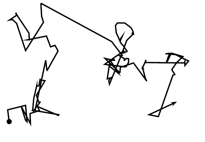
Figure 2: A series of 50 consecutive steps of Lévy flights.

In principle, flower pollination activities can occur at all scales, both local and global. But in reality, adjacent flower patches or flowers in the not-so-far-away neighborhood are more likely to be pollinated by local flower pollen than those far away. In order to mimic this feature, a switch probability (Rule 4) or proximity probability $p$ can be effectively used to switch between common global pollination to intensive local pollination. To start with, a naive value of $p=0.5$ may be used as an initially value. A preliminary parametric showed that $p=0.8$ may work better for most applications.

2.3 Multiobjective Flower Pollination Algorithm (MOFPA)

A multiobjective optimization problem with $m$ objectives can be written in general as

$$\textrm{Minimize }\;\;f_{1}(\mbox{\boldmath$x$}),f_{2}(\mbox{\boldmath$x$}),...,f_{m}(\mbox{\boldmath$x$}),$$ (7)

subject to the nonlinear equality and inequality constraints

$$h_{j}(\mbox{\boldmath$x$})=0,\quad(j=1,2,...,J),$$ (8)

$$g_{k}(\mbox{\boldmath$x$})\leq 0,\quad(k=1,2,...,K).$$ (9)

In order to use the techniques for single objective optimization or extend the methods for solving multiobjective problems, there are different approaches to achieve this. One of the simplest ways is to use a weighted sum to combine multiple objectives into a composite single objective

$$f=\sum_{i=1}^{m}w_{i}f_{i},$$ (10)

with

$$\sum_{i=1}^{m}w_{i}=1,\quad w_{i}>0,$$ (11)

where $m$ is the number of objectives and $w_{i}(i=1,...,m)$ are non-negative weights.

The fundamental idea of this weighted sum approach is that these weighting coefficients act as the preferences for these multiobjectives. For a given set of $(w_{1},w_{2},...,w_{m})$, the optimization process will produce a single point of the Pareto front of the problem. For a different set of $w_{i}$, another point on the Pareto front can be generated. With a sufficiently large number of combinations of weights, a good approximation to the true Pareto front can be obtained. It is has proved that the solutions to the problem with the combined objective (10) are Pareto-optimal if the weights are positive for all the objectives, and these are also Pareto-optimal to the original problem (7) (Miettinen 1999; Deb 2001). In practice, a set of random numbers $u_{i}$ are first drawn for a uniform distribution $U(0,1)$. Then, the weights $w_{i}$ can be calculated by normalization. That is

$$w_{i}=\frac{u_{i}}{\sum_{i=1}^{m}u_{i}},$$ (12)

so that $\sum_{i}w_{i}=1$ can be satisfied. For example, for three objectives $f_{1}$, $f_{2}$ and $f_{3}$, three random numbers/weights can be drawn from a uniform distribution $[0,1]$, and they may be $u_{1}=0.2915$, $u_{2}=0.9147$ and $u_{3}=0.6821$ in one instance of sampling runs. Then, we have $\sum_{i}=1.8883$, and $w_{1}=0.1544,w_{2}=0.4844,w_{3}=0.3612$. Indeed, $\sum_{i}w_{i}=1.000$ is satisfied.

In order to obtain the Pareto front accurately with solutions relatively uniformly distributed on the front, random weights $w_{i}$ should be used, which should be as different as possible (Miettinen 1999). From the benchmarks that have been tested, the weighted sum with random weights usually works well as can be seen below.

3 Validation and Numerical Experiments

There are many different test functions for multiobjective optimization (Zitzler and Thiele 1999; Ziztler et al. 2000; Zhang et al. 2009), but a subset of some widely used functions provides a wide range of diverse properties in terms of Pareto front and Pareto optimal set. To validate the proposed MOFPA, a subset of these functions with convex, non-convex and discontinuous Pareto fronts have been selected, including 7 single objective test functions and 4 multiobjective test functions, and two bi-objective design problems.

3.1 Single Objective Test Functions

Before proceeding to solve multiobjective optimization problems, the algorithm should first be validated by solving some well-known single objective test functions. There are at least over a hundred well-known test functions. However, there is no agreed set of test functions for validating new algorithms, though some review and literature do exist (Ackley 1987; Floudas et al. 1999; Hedar 2012; Yang 2010a). Here, a subset of seven test functions with diverse properties are used here.

The Ackley function can be written as

$$f_{1}(\mbox{\boldmath$x$})=-20\exp\Big{[}-\frac{1}{5}\sqrt{\frac{1}{d}\sum_{i=1}^{d}x_{i}^{2}}\Big{]}-\exp\Big{[}\frac{1}{d}\sum_{i=1}^{d}\cos(2\pi x_{i})\Big{]}+20+e,$$ (13)

which has a global minimum $f_{*}=0$ at $(0,0,...,0)$.

The simplest of De Jong’s functions is the so-called sphere function

$$f_{2}(\mbox{\boldmath$x$})=\sum_{i=1}^{n}x_{i}^{2},\quad-5.12\leq x_{i}\leq 5.12,$$ (14)

whose global minimum is obviously $f_{*}=0$ at $(0,0,...,0)$. This function is unimodal and convex.

Easom’s function

$$f_{3}(\mbox{\boldmath$x$})=(-1)^{d+1}\prod_{i=1}^{d}\cos(x_{i})\exp\Big{[}-\sum_{i=1}^{d}(x_{i}-\pi)^{2}\Big{]},$$ (15)

whose global minimum is $f_{*}=-1$ at $\mbox{\boldmath$x$}_{*}=(\pi,...,\pi)$ within $-100\leq x_{i}\leq 100$. It has many local minima.

Griewank’s function

$$f_{4}(\mbox{\boldmath$x$})=\frac{1}{4000}\sum_{i=1}^{d}x_{i}^{2}-\prod_{i=1}^{d}\cos(\frac{x_{i}}{\sqrt{i}})+1,\quad-600\leq x_{i}\leq 600,$$ (16)

whose global minimum is $f_{*}=0$ at $\mbox{\boldmath$x$}_{*}=(0,0,...,0)$. This function is highly multimodal.

Rastrigin’s function

$$f_{5}(\mbox{\boldmath$x$})=10d+\sum_{i=1}^{d}\Big{[}x_{i}^{2}-10\cos(2\pi x_{i})\Big{]},\quad-5.12\leq x_{i}\leq 5.12,$$ (17)

whose global minimum is $f_{*}=0$ at $(0,0,...,0)$. This function is highly multimodal.

Rosenbrock’s function

$$f_{6}(\mbox{\boldmath$x$})=\sum_{i=1}^{d-1}\Big{[}(x_{i}-1)^{2}+100(x_{i+1}-x_{i}^{2})^{2}\Big{]},$$ (18)

whose global minimum $f_{*}=0$ occurs at $\mbox{\boldmath$x$}_{*}=(1,1,...,1)$ in the domain $-5\leq x_{i}\leq 5$ where $i=1,2,...,d$.

Zakharov’s function

$$f_{7}(\mbox{\boldmath$x$})=\sum_{i=1}^{d}x_{i}^{2}+\Big{(}\frac{1}{2}\sum_{i=1}^{d}ix_{i}\Big{)}^{2}+\Big{(}\frac{1}{2}\sum_{i=1}^{d}ix_{i}\Big{)}^{4},$$ (19)

has its global minimum $f_{*}=0$ at $(0,0,...,0)$.

In order to compare the performance of FPA with other existing algorithms, each algorithm is first tested using the most widely used implementation and parameter settings. For genetic algorithms (GA), a crossover rate of $p_{\rm crossover}=0.95$ and a mutation rate of $p_{\rm mutation}=0.05$ are used (Holland 1975; Goldberg 1989; Yang 2010a). For particle swarm optimization (PSO), a version with an inertia weight $\theta=0.7$ is used, and its two learning parameters $\beta_{1}=\beta_{2}$ are set as $1.5$ (Kennedy and Eberhart 1995; Yang 2010a). Also, to ensure a fair comparison, the same population size should be used whenever possible. So $n=25$ has been used for all three algorithms.

To get some insight into the parameter settings of the FPA, a detailed parametric study has been carried out by varying $p$ from $0.05$ to $0.95$ with a step increase of $0.05$, $\lambda=1$, $1.25$, $1.5$, $1.75$, $1.9$ and $n=5,10,15,...,50$. It has been found that $n=25$, $p=0.8$, $\gamma=0.1$ and $\lambda=1.5$ works for most cases. The parameter values used for all three algorithms are summarized in Table 1.

Table 1: Parameter values for each algorithm.

PSO	$n=25,\theta=0.7$, $\beta_{1}=\beta_{2}=1.5$
GA	$n=25$, $p_{\rm crossover}=0.95,p_{\rm mutation}=0.05$
FPA	$n=25$, $\lambda=1.5$, $\gamma=0.1$, $p=0.8$

The convergence behaviour of genetic algorithms and PSO during iterations have been well studied in the literature. For FPA, various statistical measures can be obtained from a set of runs. For example, for the Ackley function $f_{1}$, the best objective values obtained during each iteration can be plotted in a simple graph as shown in Fig. 3 where a logarithmic plot shows that the convergence rate is almost exponential, which implies that the proposed algorithm is very efficient.

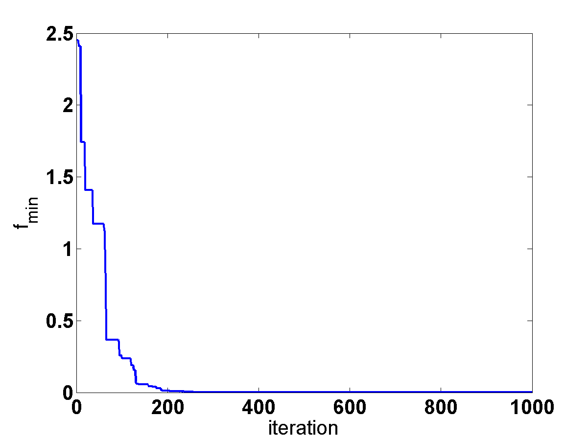
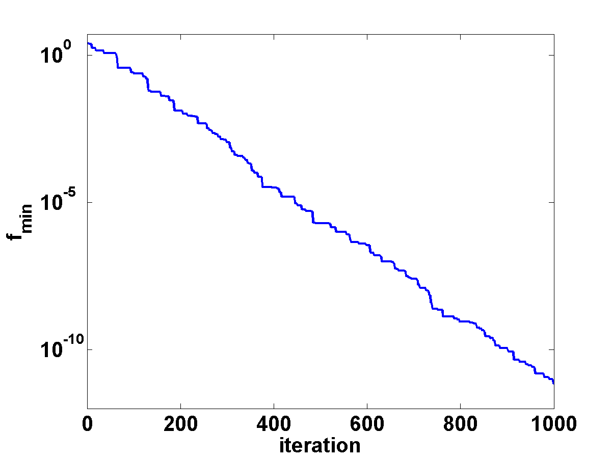
Figure 3: Convergence rate during iterations. The objective is plotted versus the iteration (left), and the same results are shown in a logarithmic scale (right).

For a fixed population size $n=25$, this is equal to the total number of function evaluations is 25,000. The best results obtained in terms of the means of the minimum values found are summarized in Table 2.

Table 2: Comparison of algorithm performance: mean values.

Functions	GA	PSO	FPA
$f_{1}$	8.29e-9	7.12e-12	5.09e-12
$f_{2}$	6.61e-15	1.18e-24	2.47e-26
$f_{3}$	-0.9989	-0.9998	-1.0000
$f_{4}$	5.72e-9	4.69e-9	1.37e-11
$f_{5}$	2.93e-6	3.44e-6	4.52e-7
$f_{6}$	8.97e-6	8.21e-8	6.19e-8
$f_{7}$	8.77e-4	1.58e-4	9.53e-5

3.2 Multiobjective Test Functions

In the rest of the paper, the parameters in MOFPA are fixed, based on a preliminary parametric study, and $p=0.8$, $\lambda=1.5$, and a scaling factor $\gamma=0.1$ are used. The population size $n=50$ and the number of iterations is set to $t=1000$. The following four functions will be tested:

• ZDT1 function with a convex front (Zitzler and Thiele 1999; Zitzler et al. 2000)

  $$f_{1}(x)=x_{1},\quad f_{2}(x)=g(1-\sqrt{f_{1}/g}),$$

  $$g=1+\frac{9\sum_{i=2}^{d}x_{i}}{d-1},\quad x_{1}\in[0,1],\;i=2,...,30,$$ (20)

  where $d$ is the number of dimensions. The Pareto-optimality is reached when $g=1$.

• ZDT2 function with a non-convex front

  $$f_{1}(x)=x_{1},\quad f_{2}(x)=g(1-\frac{f_{1}}{g})^{2},$$

  where $g$ is the same as given in ZDT1.

• ZDT3 function with a discontinuous front

  $$f_{1}(x)=x_{1},\quad f_{2}(x)=g\Big{[}1-\sqrt{\frac{f_{1}}{g}}-\frac{f_{1}}{g}\sin(10\pi f_{1})\Big{]},$$

  where $g$ in functions ZDT2 and ZDT3 is the same as in function ZDT1. In the ZDT3 function, $f_{1}$ varies from $0$ to $0.852$ and $f_{2}$ from $-0.773$ to $1$.

• LZ function (Li and Zhang, 2009; Zhang and Li, 2007)

  $$f_{1}=x_{1}+\frac{2}{|J_{1}|}\sum_{j\in J_{1}}\Big{[}x_{j}-\sin(6\pi x_{1}+\frac{j\pi}{d})\Big{]}^{2},$$

  $$f_{2}=1-\sqrt{x_{1}}++\frac{2}{|J_{2}|}\sum_{j\in J_{2}}\Big{[}x_{j}-\sin(6\pi x_{1}+\frac{j\pi}{d})\Big{]}^{2},$$ (21)

  where $J_{1}=\{j|j$ is odd $\}$ and $J_{2}=\{j|j$ is even $\}$ where $2\leq j\leq d$. This function has a Pareto front $f_{2}=1-\sqrt{f_{1}}$ with a Pareto set

  $$x_{j}=\sin(6\pi x_{1}+\frac{j\pi}{d}),\quad j=2,3,...,d,\quad x_{1}\in[0,1].$$ (22)

After generating 100 Pareto points by MOFPA, the Pareto front generated by MOFPA is compared with the true front $f_{2}=1-\sqrt{f_{1}}$ of ZDT1 (see Fig. 4).

Let us define the distance or error between the estimate Pareto front $PF^{e}$ to its corresponding true front $PF^{t}$ as

$$E_{f}=||PF^{e}-PF^{t}||^{2}=\sum_{j=1}^{N}(PF_{j}^{e}-PF_{j}^{t})^{2},$$ (23)

where $N$ is the number of points.

The variation of convergence rates or the convergence property can be viewed by plotting out the errors during iterations. As this measure is an absolute measure, which depends on the number of points. Sometimes, it is easier to use a relative measure in terms of the generalized distance

$$D_{g}=\frac{1}{N}\sqrt{\sum_{j=1}^{N}(PF_{j}-PF_{j}^{t})^{2}}.$$ (24)

The results for all the functions are summarized in Table 3, and the estimated Pareto fronts and true fronts of other functions are shown in Fig. 4 and Fig. 5. In all these figures, the vertical axis is $f_{2}$ and the horizontal axis is $f_{1}$.

3.3 Analysis of Results and Comparison

In order to compare the performance of the proposed MOFPA with other established multiobjective algorithms, we have selected a few algorithms with available results from the literature. In case of the results are not available, the algorithms have been implemented using well-documented studies and then generated new results using these algorithms. In particular, other methods are also used for comparison, including vector evaluated genetic algorithm (VEGA) (Schaffer 1985), NSGA-II (Deb et al., 2000), multiobjective differential evolution (MODE) (Babu 2007; Xue 2004), differential evolution for multiobjective optimization (DEMO) (Robič and Filipič 2005), multiobjective bees algorithms (Bees) (Pham and Ghanbarzadeh, 2007), and strength pareto evolutionary algorithm (SPEA) (Deb et al. 2002; Madavan 2002). The performance measures in terms of generalized distance $D_{g}$ are summarized in Table 4 for all the above major methods.

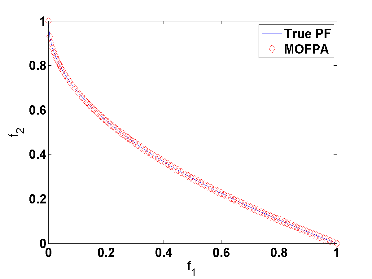
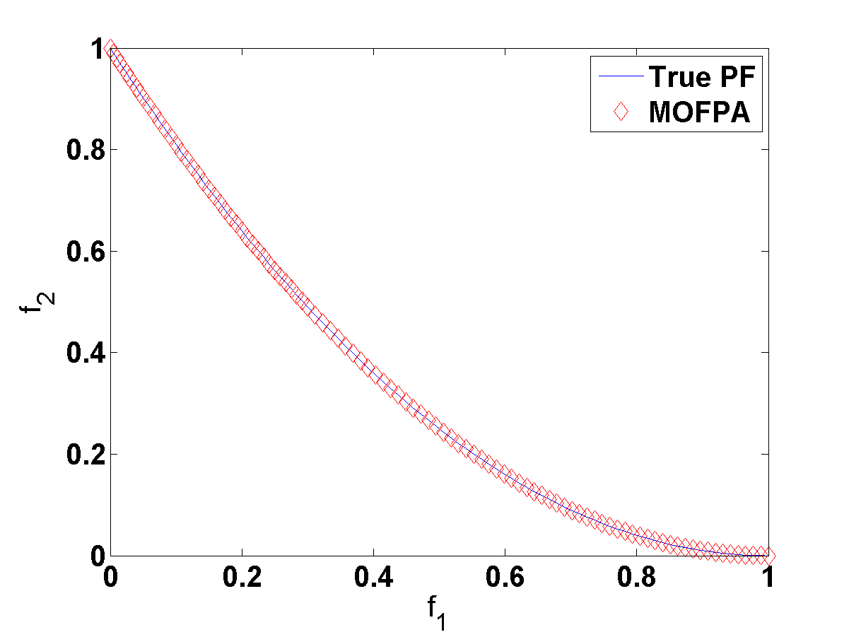
Figure 4: a) Pareto front of test function ZDT1, and b) Pareto front of test function ZDT2.

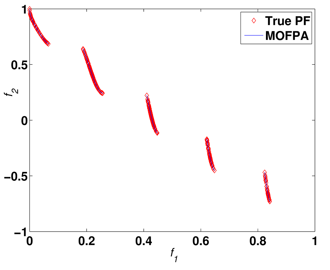
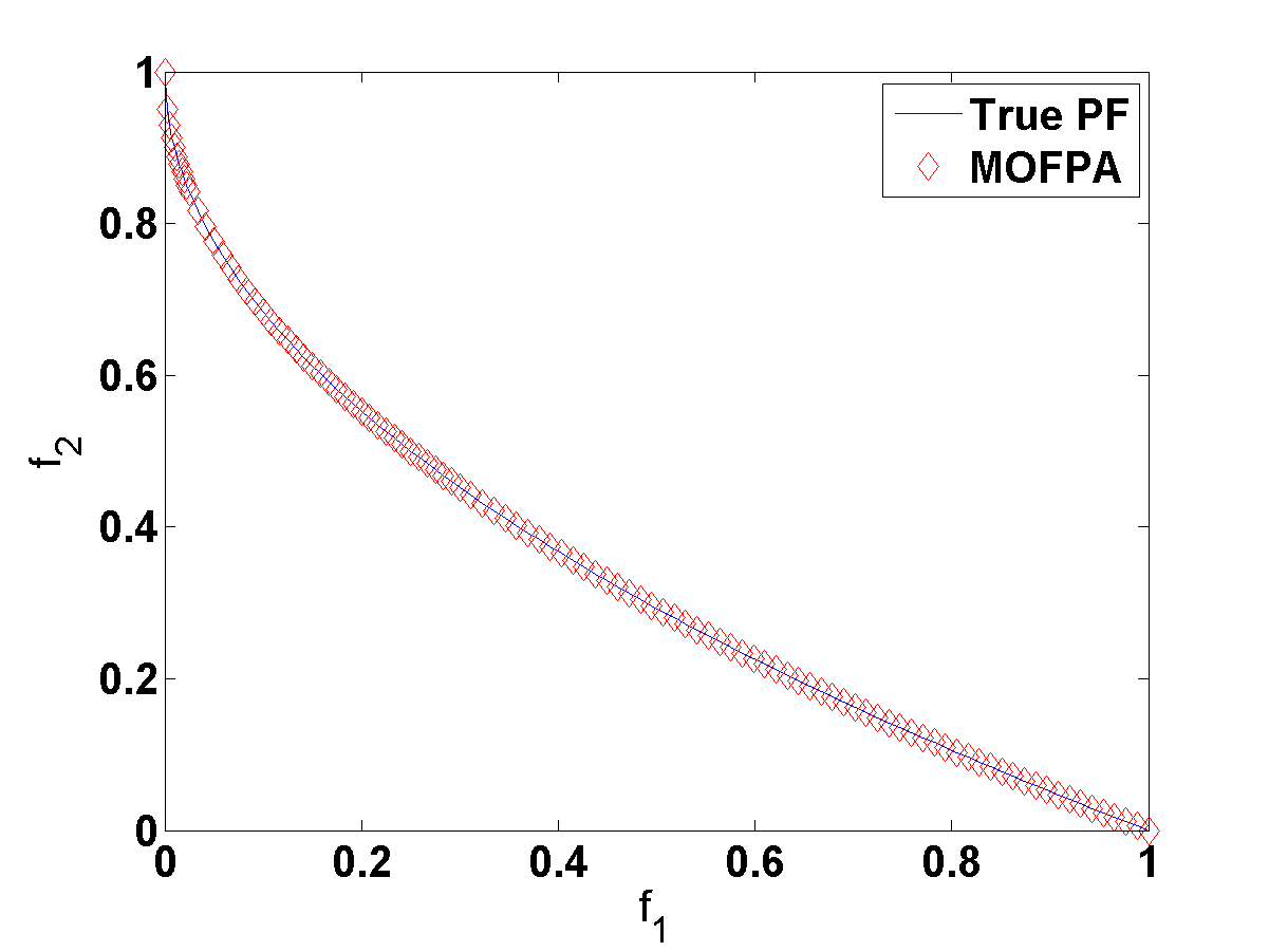
Figure 5: a) Pareto front of test function ZDT3, and b) Pareto front of test function LZ.

Table 3: Summary of results.

Functions	Errors (1000 iterations)	Errors (2500 iterations)
ZDT1	1.1E-6	3.1E-19
ZDT2	2.7E-6	4.4E-10
ZDT3	1.4E-5	7.2E-12
LZ	1.2E-6	2.9E-12

It is clearly seen from Table 4 that the proposed MOFPA obtained better results for almost all four cases.

Table 4: Comparison of $D_{g}$ for $n=50$ and $t=500$ iterations.

Methods	ZDT1	ZDT2	ZDT3	LZ
VEGA	3.79E-02	2.37E-03	3.29E-01	1.47E-03
NSGA-II	3.33E-02	7.24E-02	1.14E-01	2.77E-02
MODE	5.80E-03	5.50E-03	2.15E-02	3.19E-03
DEMO	1.08E-03	7.55E-04	1.18E-03	1.40E-03
Bees	2.40E-02	1.69E-02	1.91E-01	1.88E-02
SPEA	1.78E-03	1.34E-03	4.75E-02	1.92E-03
MOFPA	7.11E-05	1.24E-05	5.49E-04	7.92E-05

4 Structural Design Examples

Design optimization, especially design of structures, has many applications in engineering and industry. As a result, there are many different benchmarks with detailed studies in the literature (Kim et al. 1997; Pham and Ghanbarzadeh 2007; Ray and Liew 2002; Rangaiah 2008). In the rest of this paper, MOFPA will be used to solve two design case studies: design of a beam and a disc brake (Osyczka and Kundu 1995; Ray and Liew 2002; Gong et al. 2009).

4.1 Welded Beam Design

Multiobjective design of a welded beam is a classical benchmark which has been solved by many researchers (Deb 1999; Ray and Liew 2002). The problem has four design variables: the width $w$ and length $L$ of the welded area, the depth $d$ and thickness $h$ of the main beam. The objective is to minimize both the overall fabrication cost and the end deflection $\delta$.

The detailed formulation can be found in (Deb 1999; Ray and Liew 2002; Gong et al. 2009). Here the main problem is rewritten as

$$\textrm{minimise }\;f_{1}(\mbox{\boldmath$x$})=1.10471w^{2}L+0.04811dh(14.0+L),\;\textrm{ minimize }\;f_{2}=\delta,$$ (25)

subject to

$$\begin{array}[]{lll}g_{1}(\mbox{\boldmath$x$})=w-h\leq 0,\vspace{2pt}\\ \vspace{3pt}g_{2}(\mbox{\boldmath$x$})=\delta(\mbox{\boldmath$x$})-0.25\leq 0,\\ \vspace{3pt}g_{3}(\mbox{\boldmath$x$})=\tau(\mbox{\boldmath$x$})-13,600\leq 0,\\ \vspace{3pt}g_{4}(\mbox{\boldmath$x$})=\sigma(\mbox{\boldmath$x$})-30,000\leq 0,\\ \vspace{3pt}g_{5}(\mbox{\boldmath$x$})=0.10471w^{2}+0.04811hd(14+L)-5.0\leq 0,\\ \vspace{3pt}g_{6}(\mbox{\boldmath$x$})=0.125-w\leq 0,\\ \vspace{3pt}g_{7}(\mbox{\boldmath$x$})=6000-P(\mbox{\boldmath$x$})\leq 0,\end{array}$$ (26)

where

$$\begin{array}[]{ll}\sigma(\mbox{\boldmath$x$})=\frac{504,000}{hd^{2}},&Q=6000(14+\frac{L}{2}),\\ \\ D=\frac{1}{2}\sqrt{L^{2}+(w+d)^{2}},&J=\sqrt{2}\;wL[\frac{L^{2}}{6}+\frac{(w+d)^{2}}{2}],\\ \\ \delta=\frac{65,856}{30,000hd^{3}},&\beta=\frac{QD}{J},\\ \\ \alpha=\frac{6000}{\sqrt{2}wL},&\tau(\mbox{\boldmath$x$})=\sqrt{\alpha^{2}+\frac{\alpha\beta L}{D}+\beta^{2}},\\ \\ P=0.61423\times 10^{6}\;\frac{dh^{3}}{6}(1-\frac{d\sqrt{30/48}}{28}).&\end{array}$$ (27)

The simple limits or bounds are $0.1\leq L,d\leq 10$ and $0.125\leq w,h\leq 2.0$. This design problem has been solved using the MOFPA. The approximate Pareto front generated by the 50 non-dominated solutions after 1000 iterations are shown in Fig. 6. This is consistent with the results obtained by others (Ray and Liew 2002; Pham and Ghanbarzadeh 2007).

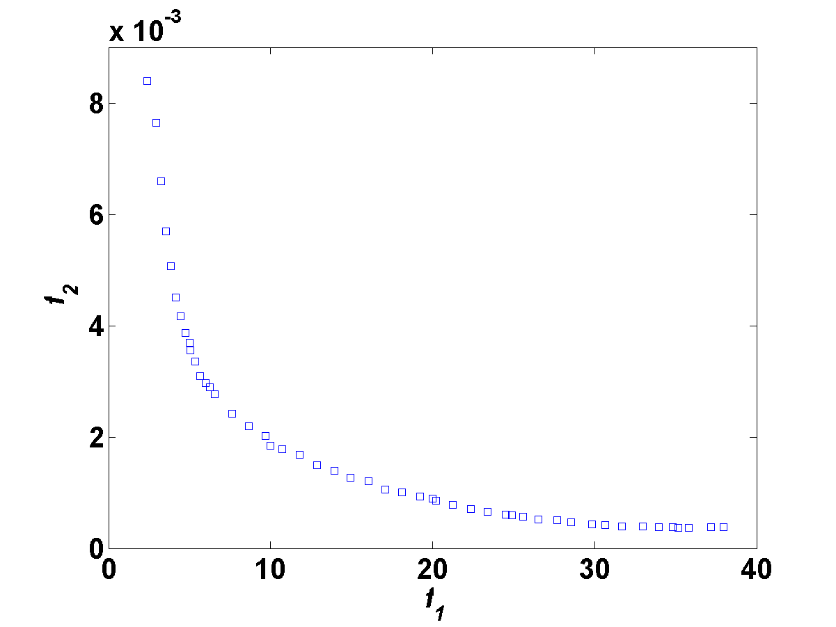
Figure 6: Pareto front for the bi-objective beam design where the horizontal axis corresponds to cost and the vertical axis corresponds to deflection.

4.2 Disc Brake Design

The objectives are to minimize the overall mass and the braking time by choosing optimal design variables: the inner radius $r$, outer radius $R$ of the discs, the engaging force $F$ and the number of the friction surface $s$. This is under the design constraints such as the torque, pressure, temperature, and length of the brake (Ray and Liew 2002; Pham and Ghanbarzadeh 2007).

This bi-objective design problem can be written as:

$$\textrm{Minimize }\;f_{1}(\mbox{\boldmath$x$})=4.9\times 10^{-5}(R^{2}-r^{2})(s-1),\quad f_{2}(\mbox{\boldmath$x$})=\frac{9.82\times 10^{6}(R^{2}-r^{2})}{Fs(R^{3}-r^{3})},$$ (28)

subject to

$$\begin{array}[]{lll}g_{1}(\mbox{\boldmath$x$})=20-(R-r)\leq 0,\\[15.0pt] g_{2}(\mbox{\boldmath$x$})=2.5(s+1)-30\leq 0,\\[15.0pt] g_{3}(\mbox{\boldmath$x$})=\frac{F}{3.14(R^{2}-r^{2})}-0.4\leq 0,\\[15.0pt] g_{4}(\mbox{\boldmath$x$})=\frac{2.22\times 10^{-3}F(R^{3}-r^{3})}{(R^{2}-r^{2})^{2}}-1\leq 0,\\[15.0pt] g_{5}(\mbox{\boldmath$x$})=900-\frac{0.0266Fs(R^{3}-r^{3})}{(R^{2}-r^{2})}\leq 0.\end{array}$$ (29)

The simple limits are

$$55\leq r\leq 80,\;75\leq R\leq 110,\;1000\leq F\leq 3000,\;2\leq s\leq 20.$$ (30)

It is worth pointing out that $s$ is discrete. In general, MOFPA has to be extended in combination with constraint handling techniques so as to deal with mixed integer problems efficiently. However, since there is only one discrete variable, the simplest branch-and-bound method is used here.

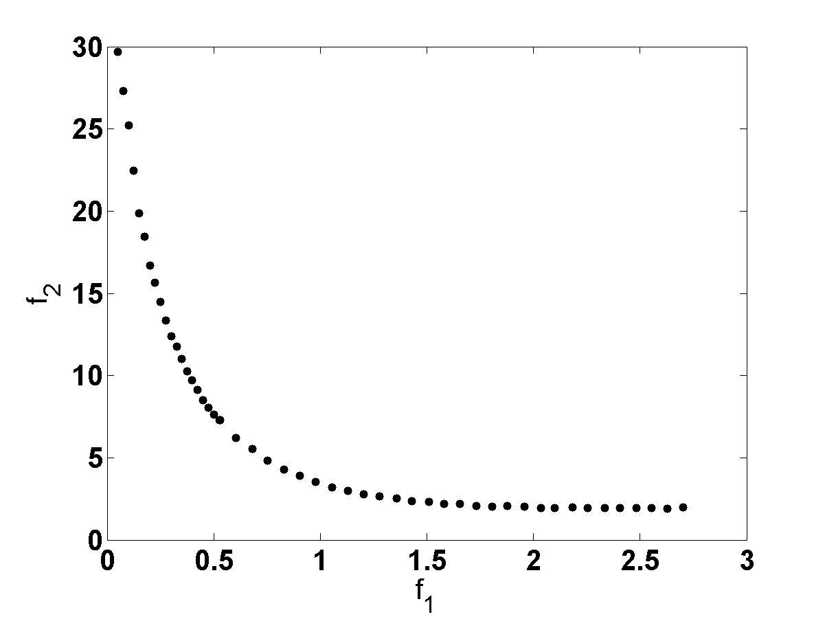
Figure 7: Pareto front of the disc brake design.

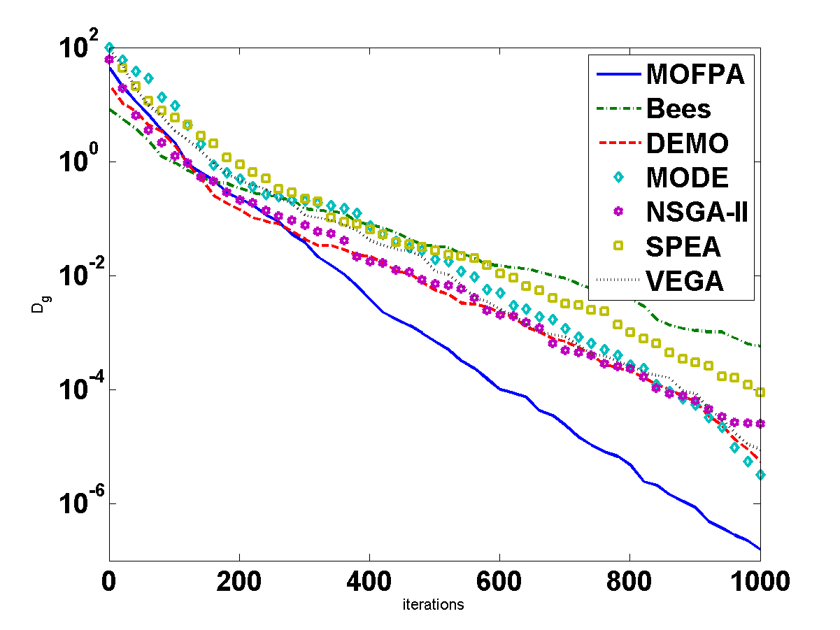
Figure 8: Convergence comparison for the disc brake design.

In order to see how the proposed MOFPA perform for the real-world design problems, the same problem has also been solved using other available multiobjective algorithms. 50 solution points are geneated using MOFPA to form an approximate to the true Pareto front after 1000 iterations, as shown in Fig. 7.

The comparison of the convergence rates is plotted in the logarithmic scales in Fig. 8. It can be seen clearly that the convergence rate of MOFPA is the highest in an exponentially decreasing way. This suggests that MOFPA provides better solutions in a more efficient way.

The above results for 11 test functions in total and two design examples suggest that MOFPA is a very efficient algorithm for multiobjective optimization. The proposed algorithm can deal with highly nonlinear, multiobjective optimization problems with complex constraints and diverse Pareto optimal sets.

5 Discussions and Conclusions

Multiobjective optimization in engineering and industry is often very challenging to solve, necessitating sophisticated techniques to tackle. Metaheuristic approaches have shown promise and popularity in recent years.

In the present work, a new algorithm, called flower pollination algorithm, has been formulated for multiobjective optimization applications by mimicking the pollination process of flowering plants. Numerical experiments and design benchmarks have shown that the proposed algorithm is very efficient with an almost exponential convergence rate, based on the comparison of FPA with other algorithms for solving multiobjective optimization problems.

It is worth pointing out that mathematical analysis is highly needed in the future work so as to gain insight into the true working mechanisms of the metaheuristic algorithms such as MOFPA. FPA has the advantages such as simplicity and flexibility, and in many ways, it has some similarity to that of cuckoo search and other algorithms with Lévy flights (Yang 2010a, 2011b), however, it is still not clear that why FPA works well. In terms of number of parameters, FPA has only one key parameter $p$ together with a scaling factor $\gamma$, which makes the algorithm easier to implement. However, the nonlinearity in Lévy flights make it difficult to analyse mathematically. It can be expected that this nonlinearity in the algorithm formulations may be advantageous to enhance the performance of an algorithm. More research may reveal the subtlety of this feature.

For multiobjective optimization, an important issue is how to ensure the solution points can distribute relatively uniformly on the Pareto front for test functions. However, for real-world design problems such as the design of a disc brake and a welded beam, the solutions are not quite uniform on the Pareto fronts, and there is still room for improvement. However, simply generating more solution points may not solve the Pareto uniformity problem easily. In fact, it is still a challenging problem on how to maintain a uniform spread on the Pareto front, which requires more studies. It may be useful as a further research topic to study other approaches for multiobjective optimization, such as the $\epsilon$-constraint method, weighted metric methods, Benson’s method, utility methods, and evolutionary methods (Miettinen 1999; Coello 1999; Deb 2001).

On the other hand, further studies can focus on more detailed parametric analysis and gain insightful of how algorithm-dependent parameters can affect the performance of an algorithm. Furthermore, the linearity in the main updating formulas makes it possible to do some theoretical analysis in terms of dynamic systems or Markov chain theories, while the nonlinearity in terms of Lévy flights can be difficult to analyze FPA exactly. All these can form useful topics for further research.

References

- [Abbass and Sarker(2002)] Abbass, H. A. and Sarker, R., 2002. “The Pareto diffential evolution algorithm.” Int. J. Artificial Intelligence Tools 11(4):531-552.
- [Ackley(1987)] Ackley, D. H., 1987. A Connectionist Machine for Genetic Hillclimbing, Kluwer Academic Publishers, (1987).
- [Babu and Gurarathi(2007)] Babu, B. V. and Gujarathi, A. M., 2007. “Multi-objective differential evolution (MODE) for optimization of supply chain planning and management”, in: IEEE Congress on Evolutionary Computation (CEC 2007), pp. 2732-2739.
- [Cagnina et al.(2008)] Cagnina, L. C., Esquivel, S. C., and Coello, C. A., 2008. “Solving engineering optimization problems with the simple constrained particle swarm optimizer”. Informatica, 32(2):319-326.
- [Coello(1999)] Coello, C. A. C., 1999. “An updated survey of evolutionary multiobjective optimization techniques: state of the art and future trends”. in: Proc. of 1999 Congress on Evolutionary Computation, CEC99, DOI 10.1109/CEC.1999.781901
- [Deb(1999)] Deb, K., 1999. “Evolutionary algorithms for multi-criterion optimization in engieering design”. in: Evolutionary Aglorithms in Engineering and Computer Science, Wiley, pp. 135-161.
- [Deb et al.(2000)] Deb, K., Pratap, A., and Moitra, S., 2000. “Mechanical component design for multiple objectives using elitist non-dominated sorting GA”, in: Proceedings of the Parallel Problem Solving from Nature VI Conference, Paris, 16-20 Sept 2000, pp. 859-868.
- [Deb(2001)] Deb, K., 2001. Multi-Objective optimization using evolutionary algorithms, John Wiley & Sons, New York.
- [Deb et al.(2002)] Deb, K., Pratap, A., Agarwal, S., Mayarivan, T., 2002. “A fast and elistist multiobjective algorithm: NSGA-II”, IEEE Trans. Evol. Computation, 6(2):182-197.
- [Eusuff(2006)] Eusuff, M., Lansey, K., Pasha, F., (2006). “Shuffled frog-leaping algorithm: a memetic metaheuristic for discrete optimization”, Engineering Optimization, 38(2):129-154.
- [Floudas et al.(1999)] Floudas, C. A., Pardalos, P. M., Adjiman, C. S., Esposito, W. R., Gumus, Z. H., Harding, S. T., Klepeis, J. L., Meyer, C. A., Scheiger, C. A., Handbook of Test Problems in Local and Global Optimization, Springer, (1999).
- [Gandomi et al.(2012)] Gandomi, A. H., Yang, X. S., Talatahari, S., and Deb, S., 2012. “Coupled eagle strategy and differential evolution for unconstrained and constrained global optimization.” Computers & Mathematics with Applications, 63(1):191–200.
- [Gandomi and Yang(2011)] Gandomi, A. H., and Yang, X. S., 2011. “Benchmark problems in structural optimization.” in: Computational Optimization, Methods and Algorithms (Eds. S. Koziel and X. S. Yang), Study in Computational Intelligence, SCI 356:259-281, Springer, Germany.
- [Geem et al.(2001)] Geem, Z. W., Kim, J. H., and Loganathan, G. V., 2001. “A new heuristic optimization: Harmony search”, Simulation, 76(2):60-68.
- [Geem(2006)] Geem, Z. W., 2006. “Optimal cost design of water distribution networks using harmony search.” Engineering Optimization, 38(3):259-280.
- [Geem(2009)] Geem, Z. W., 2009. Music-Inspired Harmony Search Algorithm: Theory and Applications, Springer, Heidelberg.
- [Glover(2007)] Glover, B. J., 2007. Understanding Flowers and Flowering: An Integrated Approach, Oxford University Press, Oxford, UK.
- [Goldberg(1989)] Goldberg, D. E., 1989. Genetic Algorithms in Search, Optimisation and Machine Learning, Reading, Mass.: Addison Wesley (1989).
- [Gong et al.(2009)] Gong, W. Y., Cai, Z. H., Zhu, L., 2009. “An effective multiobjective differential evolution algorithm for engineering design.” Struct. Multidisc. Optimization, 38(2):137-157.
- [He et al.(2004)] He, S., Prempain, E., and Wu, Q. H., 2004. “An improved particle swarm optimizer for mechanical design optimization problems.” Engineering Optimization, 36(5):585-605.
- [Hedar(2013)] Hedar, A., 2013. Test function web pages, http://www-optima.amp.i.kyoto-u.ac.jp /member/student/hedar/Hedarfiles/TestGOfiles/Page364.htm [Accessed on 1 June 2013.]
- [Holland(1975)] Holland, J., 1975. Adaptation in Natural and Artificial Systems, University of Michigan Press, Ann Anbor.
- [Huang(1996)] Huang, G. H., 1996. “IPWM: An interval parameter water quality management model.” Engineering Optimization, 26(1):79-103.
- [Kennedy and Eberhart(1995)] Kennedy, J., and Eberhart, R. C., 1995. “Particle swarm optimization.” Proc. of IEEE International Conference on Neural Networks, Piscataway, NJ. pp. 1942-1948.
- [Kim et al.(1997)] Kim, J. T., Oh, J. W. and Lee, I. W., 1997. “Multiobjective optimization of steel box girder brige.” in: Proc. 7th KAIST-NTU-KU Trilateral Seminar/Workshop on Civil Engineering, Kyoto, Dec 1997.
- [Lee et al.(2005)] Lee, K. S., Geem, Z. W., Lee, S.-H., Bae, K.-W., 2005. “The harmony search heuristic algorithm for discrete structural optimization.” Engineering Optimization, 37(7):663-684.
- [Li and Zhang(2009)] Li, H. and Zhang, Q. F., 2009. “Multiobjective optimization problems with complicated Paroto sets, MOEA/D and NSGA-II.” IEEE Trans. Evol. Comput., 13:284–302.
- [Madavan(2002)] Madavan, N. K., 2002. “Multiobjective optimization using a pareto differential evolution approach.” in: Congress on Evolutionary Computation (CEC’2002), Vol. 2, New Jersey, IEEE Service Center, pp. 1145–1150.
- [Mantegna(1994)] Mantegna, R. N., 1994. “Fast, accurate algorithm for numerical simulation of Lévy stable stochastic process.” Physical Review E, 49:4677–4683.
- [Marler(2004)] Marler, R. T. and Arora, J. S., 2004. “Survey of multi-objective optimization methods for engineering.” Struct. Multidisc. Optim., 26:369–395.
- [Miettinen(1999)] Miettinen, K., 1999. Nonlinear Multiobjective Optimization (International Series in Operations Research & Management Science), Kluwer Academic Publishers, Massachusetts.
- [Osyczka and Kundu(1995)] Osyczka, A. and Kundu, S., 1995. “A genetic algorithm-based multicriteria optimization method.” Proc. 1st World Congr. Struct. Multidisc. Optim., Elsevier Sciencce, pp. 909-914.
- [Pavlyukevich(2007)] Pavlyukevich, I., 2007. “Lévy flights, non-local search and simulated annealing.” J. Computational Physics, 226:1830–1844.
- [Pham and Ghanbarzadeh(2007)] Pham, D. T. and Ghanbarzadeh, A., 2007. “Multi-Objective Optimisation using the Bees Algorithm.” in: 3rd International Virtual Conference on Intelligent Production Machines and Systems (IPROMS 2007), Whittles, Dunbeath, Scotland.
- [Rangaiah(2008)] Rangaiah, G., 2008. Multi-objective Optimization: Techniques and Applications in Chemical Engineering, World Scientific Publishing, Singapore.
- [Ray and Liew(2002)] Ray, L. and Liew, K. M., 2002. “A swarm metaphor for multiobjective design optimization.” Engineering Optimization, 34(2):141–153.
- [Reyes-Sierra and Coello(2006)] Reyes-Sierra, M. and Coello, C. A. C., 2006. “Multi-objective particle swarm optimizers: A survey of the state-of-the-art.” Int. J. Comput. Intelligence Res., 2(3):287–308.
- [Robič and Flipič(2005)] Robič, T. and Filipič, B., 2005. “DEMO: differential evolution for multiobjective optimization.” in: EMO 2005 (eds. C. A. Coello Coello), LNCS 3410:520–533.
- [Schaffer(1985)] Schaffer, J. D., 1985. “Multiple objective optimization with vector evaluated genetic algorithms.” in: Proc. 1st Int. Conf. Genetic Aglorithms, pp. 93–100.
- [Science Daily(2001)] Science Daily, 2001. “Oily Fossils provide clues to the evolution of flowers”, Science Daily, 5 April 2001. http://www.sciencedaily.com/releases/2001/04/010403071438.htm
- [Walker(2009)] Walker, M., 2009. “How flowers conquered the world”, BBC Earth News, 10 July 2009. http://news.bbc.co.uk/earth/hi/earth_news/newsid_8143000/8143095.stm
- [Waser(1986)] Waser, N. M., 1986. “Flower constancy: definition, cause and measurement.” The American Naturalist, 127(5):596-603.
- [Xue(2004)] Xue, F., 2004. Multi-objective differential evolution: theory and applications, PhD thesis, Rensselaer Polytechnic Institute.
- [Yang(2010a)] Yang, X. S., 2010a. Engineering Optimization: An Introduction with Metaheuristic Applications, John Wiley and Sons, USA.
- [Yang(2010b)] Yang, X. S., 2010b. “A new metaheuristic bat-inspired algorithm.” in: Nature-Inspired Cooperative Strategies for Optimization (NICSO 2010), SCI 284:65–74.
- [Yang(2011a)] Yang, X. S., 2011a. “Bat algorithm for multi-objective optimisation.” Int. J. Bio-Inspired Computation, 3(5):267–274.
- [Yang(2011b)] Yang, X. S., 2011b. “Review of meta-heuristics and generalised evolutionary walk algorithm.” Int. J. Bio-Inspired Computation, 3(2):77–84.
- [Yang and Gandomi(2012)] Yang, X. S. and Gandomi, A. H., 2012. “Bat algorithm: a novel approach for global engineering optimization.” Engineering Computations, 29(5):464–483.
- [Yang(2012)] Yang, X. S., 2012. “Flower pollination algorithm for global optimization.” in: Unconventional Computation and Natural Computation, Lecture Notes in Computer Science, 7445:240–249.
- [Yang et al.(2013)] Yang, X. S., Karamanoglu, M., He, X. S., 2013. “Multi-objective flower algorithm for optimization.” Procedia Computer Science, 18:861–868.
- [Zhang et al.(2009)] Zhang, Q. F., Zhou, A. M., Zhao, S. Z., Suganthan, P. N., Liu, W., Tiwari, S., 2009. “Multiobjective optimization test instances for the CEC 2009 special session and competition.” Technical Report CES-487, University of Essex, UK.
- [Zhang and Li(2007)] Zhang, Q. F. and Li, H., 2007. “MOEA/D: a multiobjective evolutionary algorithm based on decomposition.” IEEE Trans. Evol. Comput., 11(6):712–731.
- [Zitzler and Thiele(1999)] Zitzler, E. and Thiele, L., 1999. “Multiobjective evolutonary algorithms: A comparative case study and the strength pareto approach.” IEEE Evol. Comp., 3(4):257–271.
- [Zitzler et al.(2000)] Zitzler, E., Deb, K., and Thiele, L., 2000. “Comparison of multiobjective evolutionary algorithms: Empirical results.” Evol. Comput., 8(2):173–195