Inexpensive discrete atomistic model technique for studying excitations on infinite disordered media: the case of orientational glass ArN₂

Abstract

Excitations of disordered systems such as glasses are of fundamental and practical interest but computationally very expensive to solve. Here we introduce a technique for modeling these excitations in an infinite disordered medium with a reasonable computational cost. The technique relies on a discrete atomic model to simulate the low-energy behavior of an atomic lattice with molecular impurities. The interaction between different atoms is approximated using a spring like interaction based on the Lennard Jones potential but can be easily adapted to other potentials. The technique allows to solve a statistically representative number of samples with a minimum of computational expense, and uses a Monte-Carlo approach to achieve a state corresponding to any given temperature. This technique has already been applied successfully to a problem with interest in condensed matter physics: the solid solution of N₂ in Ar.

keywords: glasses; low temperature; atomic modeling; Ar:N2; two-level systems; disordered lattices, universality

1 Introduction

Excitations of disordered systems such as glasses are computationally very expensive to solve. The first difficulty arises because molecular, atomic and quantum effects are so important that one needs an atomistic description to understand the origin of the thermal and mechanical properties at low temperature. Nevertheless, and contrary to the situation in ordered crystals, it is not merely difficult to calculate the quantum ground state but there is actually no real physical ground state that the system can reach experimentally at low enough temperatures. Instead, there is just a complicated Potential Energy Landscape where the low-energy state depends on the thermal history if the system. It is also impossible to apply real periodic boundary conditions, as the disorder itself is not periodic, so border effects have to be suppressed by using large fragments. What is worse, a critical parameter that determines the properties of such systems is its composition, so the study needs to be performed at each concentration of impurities.

Disordered systems actually quite common, so the problem is of general interest. Indeed, for many real solids progressively lowering the temperature produces an apparently infinite series of ever more weak interactions, and solid-state physicists do not presently understand the basic structure of the low-energy states of most systems, excluding the most simple ones.

In this context, a Two Level System (TLS) corresponds formally to a related pair of local minima, or a double-well potential on the Potential Energy landscape (PEL). These minima need to have an small energy difference and distance to allow for tunneling  [1]. TLSs are believed to be the origin of certain universal properties in disordered solids, and also the cause of $1/f$ noise in superconducting qubits, a bottleneck in Quantum Technologies. Thus there is interest in studying them; a crucial step being, of course, determining their nature,  [2, 3, 4, 5]. For the reasons aforementioned, computer simulations are strongly limited and usually only rather small systems are used to analyze the PEL and TLS properties. This may give rise to significant finite size effects and may strongly influence the properties of the TLS obtained by computer simulations. The computational cost also imposes limitations on the possibility of obtaining enough results to have statistic significance, affecting the validity of the results.

In this work we introduce a technique for modeling TLS that allows to model a infinite disordered medium with a reasonable computational cost. The technique relies on a discrete atomic model to simulate the low-energy behavior of an atomic lattice with impurities (displaying TLSs). The discrete model is based on the equilibrium equations of atomic interaction forces  [6, 7] as the equilibrium state of the lattice corresponds to the minimal value of the total potential energy of the atomic structure and uses a Monte-Carlo method to set the working temperature. As the numerical formulation is similar to other well known classical formulations, like the finite element method, the introduction of boundary conditions is simplified. The density of impurities can thus be iteratively increased up to the desired level by adding impurities at random positions. A number of independent histories are stored to achieve a statistically representative set of random configurations.

To illustrate the method, we focus our study on the solid solution of the nitrogen molecule N₂ in an Ar lattice, where the TLSs are expected to be closely related to different orientations of the N₂ molecules. As no relevant three-dimensional-specific effects are expected in this system, for ease of visualization we describe here only the study in two dimensions. Displaying only weak van der Waals forces and being an intriguing system in the context of universality of low-temperature properties of disordered systems, Ar:N₂ is particularly well-suited for exemplifying our approach, which is extensible to many systems of different nature. The present work deals mainly with the new methodology, while the physical consequences of the results we obtain are presented elsewhere  [8].

2 Potential description for the discrete atomic model

We use a discrete atomic model to compute and simulate the equilibrium of an atomic Ar lattice including N₂ impurities. The equilibrium state of the lattice corresponds to the minimal value of the total potential energy of the atomic structure. This model is based on the equilibrium equations of atomic interaction forces  [6, 7]. The model assumes interactions between each atomic pair which are approximated using a non linear spring model [7, 9], even if the potential energy can be described using different equations depending on distance between each 2, 3 or many atoms. For sake of simplicity, we based the approach on the Lennard Jones potential  [10], as it is one of the most extensively used for fluids and solids  [11, 12, 13] and also for large systems  [14].

The Lennard Jones 6-12 function is used to describe the interaction between two atoms of the lattice. The potential energy of the Lennard-Jones function is expressed as

$$V_{ij}(r_{ij})=4\varepsilon\left[\left(\frac{\sigma}{r_{ij}}\right)^{12}-\left(\frac{\sigma}{r_{ij}}\right)^{6}\right]$$ (1)

where $\varepsilon$ denotes the well depth and $\sigma$ the zero-potential distance between two atoms. $r_{ij}$ is the existing distance between the interacting atoms $i$ and $j$. It is well known that the Lennard-Jones interactions decrease rapidly as distance increases, the potential becoming negligible if the distance $r_{ij}$ is much greater than zero-potential distance. The usual choice for the cut-off distance, which we adopt, is 2.5$\sigma$.

The former description corresponds to the existing interaction between two Ar, or between a Ar and N atom. The potential parameters (energies in Hartree, distances in Bohr radius) are $\varepsilon_{Ar-Ar}=3.7936*10^{-4}eH$, $\sigma_{Ar-Ar}=6.3302r_{B}$,  [15, 16] , $\varepsilon_{Ar-N}=2.1263*10^{-4}eH$, $\sigma_{Ar-N}=6.3306r_{B}$  [15, 17].

The N-N interaction deserve some extra cautions, as we need to reproduce both the intramolecular behavior of the N₂ molecule, with a very stiff and rather short covalent bond, and the intermolecular interaction between two molecules, which is weak and similar to the Ar-Ar interaction. We do this by using a potential composed by two very different LJ functions. Of course, the transition between the two potentials has to be chosen carefully to avoid numerical instabilities or mathematical artifacts. With these considerations the potential for N-N interactions is chosen as: (2)

$$V^{TLS}_{ij}(r_{ij})=4\left\{\begin{array}[]{ccc}\varepsilon^{TLS}\left[\left(\frac{\sigma^{TLS}}{r_{ij}}\right)^{12}-\left(\frac{\sigma^{TLS}}{r_{ij}}\right)^{6}\right]&&\text{region 1}\\ \\ \varepsilon^{TLS}_{W}\left[\left(\frac{\sigma^{TLS}_{W}}{r_{ij}}\right)^{12}-\left(\frac{\sigma^{TLS}_{W}}{r_{ij}}\right)^{6}\right]&&\text{region 2}\end{array}\right.$$ (2)

region 1 indicates the region outside the bond link of the N₂ molecule and regions 2 indicates the bond affected region inside the N₂ molecule, which produces the potential well and also the TLS effect, superscript $TLS$ remarks the TLS association, subscript $W$ indicates the parameters for this inner potential well which is considered deeper. The region 2 definition is controlled using a cut off function in function of $\sigma^{TLS}_{W}$, regions 1 starts after this cut off for regions 2; beyond the cut off distance $2.5\sigma_{TLS}$ the potential is defined as zero. Considering the Ar:N₂ mixture, we will have the following parameter $\varepsilon_{N-N}=\varepsilon^{TLS}_{W}=0.3601eH$, $\sigma_{N-N}=\sigma^{TLS}_{W}=2.0749r_{B}$,  [17], $\varepsilon_{N_{2}-N_{2}}=\varepsilon^{TLS}=1.3916*10^{-4}eH$, $\sigma_{N_{2}-N_{2}}=\varepsilon^{TLS}=6.3136r_{B}$ , [18]; the inner cut-off distance is $2.43\sigma_{N-N}$ that is where region 2 ends. The qualitative behavior of potentials for the typical interatomic/intermolecular vs intramolecular potential is shown in Fig. 1.

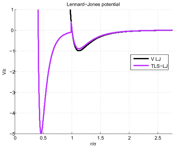
Figure 1: Qualitative illustration of the potentials between Ar atoms (V LJ) and double potential to reproduce both the covalent bond and the weaker interactions of N₂ molecules using the Lennard-Jones potential (TLS-LJ). For clarity we choose $\sigma^{TLS}=\sigma$, $\varepsilon^{TLS}=0.9\varepsilon$, $\sigma^{TLS}_{W}=0.41\sigma$, $\varepsilon^{TLS}_{W}=10\varepsilon$. Of course, in the actual calculations the potential for the covalent bond would be much deeper.

3 Spring-like description for the discrete atomic model

Our model assumes spring like bonded atoms on static equilibrium. That is, the interaction between each atomic pair can be approximated using a spring model as in  [7, 9]. More exactly, the Lennard-Jones bond behavior is approximated as a non-linear spring:

$$\textbf{f}_{ij}=\textbf{k}_{ij}(\textbf{u}_{i}-\textbf{u}_{j})$$ (3)

The interaction forces between each pair of atoms in the lattice with non zero potential are computed from the potential function, that is:

$$\textbf{f}_{ij}(r_{ij})=-\frac{\partial V(r_{ij})}{\partial r_{ij}}=\frac{4\varepsilon}{r_{ij}}\left[\left(-12\frac{\sigma}{r_{ij}}\right)^{12}+6\left(\frac{\sigma}{r_{ij}}\right)^{6}\right]\textbf{n}_{ij}$$ (4)

However in practice we will use the distance vector between the constitutive atoms of the pair $\textbf{r}_{ij}$ instead of the direction, as in  [7] to achieve the following expression:

$$\textbf{f}_{ij}(r_{ij})=f_{ij}\frac{\textbf{r}_{ij}}{r_{ij}}$$ (5)

$$\textbf{f}_{ji}=-\textbf{f}_{ij}$$

$$f_{ij}=\frac{4\varepsilon}{r_{ij}}\left[\left(-12\frac{\sigma}{r_{ij}}\right)^{12}+6\left(\frac{\sigma}{r_{ij}}\right)^{6}\right]$$

We inferred $\textbf{k}_{ij}$ from the slope of the force. However, if distance $r_{ij}$ is greater than 1.244 $\sigma$, the slope is negative. The introduction of a negative stiffness may induce some numerical problems and, for our case, lacks of physical interpretation, hence the absolute value of the slope is used. No special treatment is done for the special case of $1.244\sigma$ where the slope is zero, as the possibility of it becoming a explosive point is almost negligible. The Exact expression for the stiffness is then

$$\textbf{k}_{ij}(r_{ij})=\left|k_{ij}\frac{\textbf{r}_{ij}}{r_{ij}}\right|$$ (6)

$$k_{ij}=\left|\frac{\partial f_{ij}}{\partial r_{ij}}\right|=\left|\frac{4\varepsilon}{r_{ij}}\left[\left(156\frac{\sigma}{r_{ij}}\right)^{12}-42\left(\frac{\sigma}{r_{ij}}\right)^{6}\right]\right|$$

The aspect of the results for a typical Lennard-Jones are shown in Fig. 2. The force and string modulus for the TLS are derived directly in each region from the corresponding potential using Eq. (5) and Eq. (6), respectively.

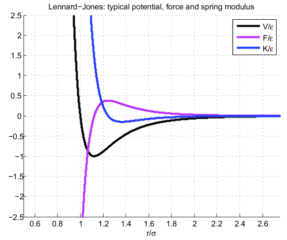
Figure 2: Aspect of the potential, force and spring moduli for a typical Lennard-Jones potential.

If we accept the expression (3) as representative for the interaction between every pair of atoms of the atomic system, we can consider the following expression:

$$\textbf{K}\textbf{U}=\textbf{F}$$ (7)

where U is the displacement vector for all the atoms of the system. That is: it is a vector of size $n_{at}\ast n_{dm}$, where $n_{at}$ is the number of atoms and $n_{dm}$ the dimension of the system. Hence, if we consider the atom at position $i$ and ($i_{x}$,$i_{y}$,$i_{z}$) indicates each space direction, then the displacement of the atom $i$ is given by

$$\textbf{U}_{i}=\textbf{u}_{i}=\begin{vmatrix}u_{i_{x}}\\ u_{i_{y}}\\ u_{i_{z}}\end{vmatrix}$$ (8)

The components of the force vector F are built adding the force terms of each possible pair of atoms

$$\textbf{F}^{e}_{i} =\textbf{f}_{ij}=\begin{vmatrix}f_{ij_{x}}\\ f_{ij_{y}}\\ f_{ij_{z}}\end{vmatrix}$$ (9)

$$\textbf{F}^{e}_{j} =\textbf{f}_{ij}=-\begin{vmatrix}f_{ij_{x}}\\ f_{ij_{y}}\\ f_{ij_{z}}\end{vmatrix}$$

Finally the stiffness matrix, of size $(n_{at}\ast n_{dm})\times(n_{at}\ast n_{dm})$ is formed by adding the elemental stiffness matrix defined for each pair of atoms $ij$, definition which practically neglects the effect of a zero value for a pair of atoms with a distance of $1.244\sigma$. That is:

$$\begin{pmatrix}K^{e}_{ii_{xx}}&K^{e}_{ii_{xy}}&K^{e}_{ii_{xz}}\\ K^{e}_{ii_{yx}}&K^{e}_{i_{yy}}&K^{e}_{ii_{yz}}\\ K^{e}_{ii_{zx}}&K^{e}_{ii_{zy}}&K^{e}_{ii_{zz}}\end{pmatrix} =\begin{pmatrix}k_{ij_{x}}&0&0\\ 0&k_{ij_{y}}&0\\ 0&0&k_{ij_{z}}\end{pmatrix}$$ (10)

$$\begin{pmatrix}K^{e}_{ij_{xx}}&K_{ij_{xy}}&K^{e}_{ij_{xz}}\\ K^{e}_{ij_{yx}}&K^{e}_{ij_{yy}}&K^{e}_{ij_{yz}}\\ K^{e}_{ij_{zx}}&K^{e}_{ij_{zy}}&K^{e}_{ij_{zz}}\end{pmatrix} =\begin{pmatrix}-k_{ij_{x}}&0&0\\ 0&-k_{ij_{y}}&0\\ 0&0&-k_{ij_{z}}\end{pmatrix}$$

The expression (7), and its spring like physical meaning allows to introduce boundary conditions as in other classical numerical model, for example, as in the finite element framework.

If the system is at equilibrium then the PEL shows a minimum state, where the resultant forces and displacements are zero. While this is not necessarily a real physical state, it could be considered as an average description of an atomic system at low temperatures. If the PEL is not on a minimum state then there are resultant forces which produce a displacement of the atoms, U, from the initial position to another, likely more stable one. We can then update the position using the information on U and recompute U using (7) where K and F corresponds to the updated position. We iterate the process until the maximum of the absolutes values of U is below a tolerance. Then we can accept that the system has arrived to equilibrium and no further displacement occurs. For our example we fix that tolerance as $0.01r_{B}$.

We implemented two exit conditions for non-convergence of the iterative process. The first one is limiting the number of iterations, in our case 200, and the second one is using the maximum of the absolute values of U, as we can consider that over a certain displacement, in our case $1.5r_{B}$, the configuration of the system has changed beyond control. In either case we consider that the calculation did not converge and we reject the results. This exit conditions achieve a considerable gain in computation velocity at the cost of not being able to deal with some of the most unstable starting positions.

4 Lattice and impurities

We want to minimize the finite size effect on modelization, at least on a controlled central region, thus if the border influence can be neglected then the infinite medium assumption for our system can be accepted. The finite size effect is directly related to the model size, thus we evaluate it by comparing different model sizes. We use 5x5, 9x9 and 13x13 pure Ar lattice with hexagonal structure and the distances corresponding to the experimental crystal structure [15]. We analyze the effect of the finite lattice size considering the presence of impurities. Four different cases with two N₂ impurities are modeled. The impurities are placed on different positions but close to the center region, as shown in Fig. 3 and each N₂ is rotated 30 degrees, independently, to check the possible influence of orientation. That makes a total of 144 computations for each lattice size.

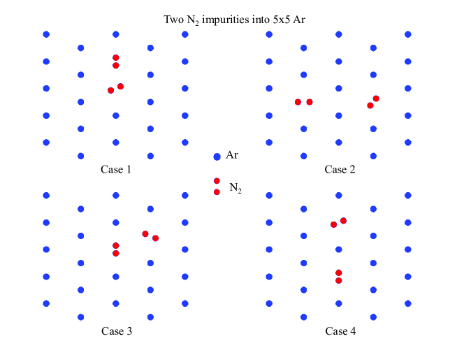
Figure 3: Location of two impurities for checking the lattice finite size effect.

The three systems with lowest energy for each lattice size for the former configurations, which are shown on Fig 4, are compared. We can observe that for the 5x5 lattice the states are not the same as for the 9x9 and 13x13 cases. Moreover the difference of energy between each lowest energy state for the 9x9 and 13x13 lattice sizes agree. Consequently we can accept that in the central region of a 9x9 lattice the size effects are negligible. Besides the energy analysis, the whole computation for the 9x9 lattice took less than 30 minutes on a 2 gigabyte and 2,53 GHz laptop running under windows 7. Because of its feasible computation time, the 9x9 lattice size is a suitable candidate for statistical studies.

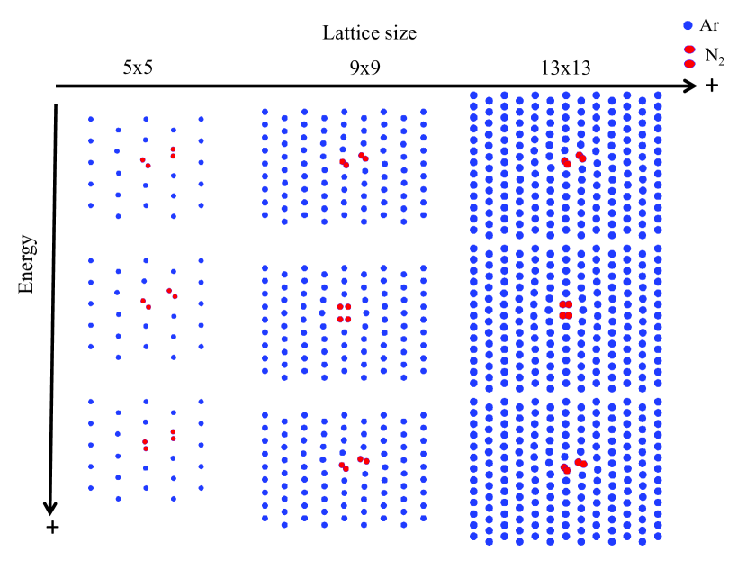
Figure 4: Configurations with the minimum energy for the different lattice sizes.

5 Disordered infinite medium. Excitations for Tunneling effect by TLS-phonon coupling.

The lattice size is chosen as a compromise between avoiding the border effect on the central region and having a feasible computationally time. We start from a 9x9 pure Ar lattice with hexagonal structure and the distances corresponding to the experimental crystal structure [15]. In all our calculations the external Ar frame is kept intact and only the inner 8x8 lattice is relaxed. Similarly, only the inner 8x8 lattice is populated by N₂ impurities.

The impurity density is increased iteratively adding one N₂ per step. Particularly, the concentration of N₂ is increased by adding a randomly located and randomly oriented N₂ to the relaxed region of a previous configuration. For increasing the stability of the system, the lattice intersite distance is slightly modified with each N₂ addition, in accordance with the real density of Ar:N₂ mixtures. After the addition of one N₂ the system is relaxed. That procedure simplifies the random enrichment of the lattices as it starts from a stable configuration and only a N₂ is added in each step. Examples of this process can be observed for different densities on Fig. 5.

If the system relaxing converges we save the results, and repeat the procedure until we have saved 50 stable lattices with the same number of N₂ molecules in different positions. For the first N₂ added to the pristine Ar lattice, we keep the 50 lattices, which we will use as starting steps for 50 independent iterative procedures. For each subsequent iteration addition of N₂ to each of these 50 independent histories, we keep only the lattice with the lowest energy. This produces 50 independent and relatively low-energy configurations for each Ar:N₂ ratio. That is for each Ar:N₂ ratio we check 50x50 stable configurations taking the lowest energy configuration for each family as previous configuration for the following substep. All the non stable configurations are discarded. without further computations.

The maximum achieved Ar:N₂ ratio is 0.2:0.8, meaning 80% of inner 7x7 lattice positions are N₂. To further decrease the energy and approximate the real ground state, we perform a Monte-Carlo cooling  [19, 20]: for each state we rotate randomly and sequentially each N₂ and keep the new state if the new configuration converges to a lower energy. We perform 25 sequential sweeps of each lattice. This decreases the energy an average of $0.14eV$.

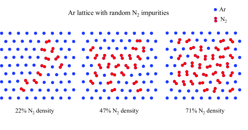
Figure 5: Configurations corresponding to local energy minima obtained as described in the text for different Ar:N₂ ratios.

The total number of stable configurations for the 9x9 Ar:N₂ were over 97 000 and, including the MC cooling, took about 30 days on a computer with 4 cpus. In comparison, in [5], a computer with 200 cpus need the same time for a sample of 3000 4x4x4 configurations or 5000 8x8 configurations of KBr:CN.

We obtained a set of histories for 9x9 Ar lattices with hexagonal structure and different concentration of N₂ randomly placed. The Monte-Carlo cooling process also lead the system to a ground like state. All this process allows to accept the results as representative of a disordered medium. However, the goal is the study of the coupling of the different TLSs excitations in a infinite lattice, therefore only the seven central atoms of the lattice are considered to minimize border effects.

Three types of possible TLSs coupling are considered for this seven central positions, one which corresponds to a tunneling process where an Ar atom and an N₂ molecule exchange positions. This we label as Ar-tunnel, the second excitation corresponds to an orientation change such that an N₂ adopts the orientation of a neighboring, non-parallel N₂, and label this as rotation. The third excitations corresponds to the exchange of orientation of two non-parallel N₂ and is refereed as flip-flop. An representation of the central seven atoms and the excitations are shown in Fig. 6. The excited state is only accepted if (a) its relaxation process converges and (b) it does not reproduce geometry of its ground state after the relaxation.

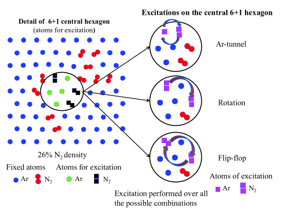
Figure 6: Detail of the excitations

The distribution of TLSs with a N₂ density up to 20% is shown in Fig. 7. The comparison of the histograms allows to identify which excitations is expected at lower density. As seen in Fig. 7(a), and as expected statistically, Ar-N₂ tunneling process are more likely at low N₂ densities compared with processes that require two N₂ molecules. In this case we see a sharp peak of excitations at near-zero energy, corresponding to the cases where there is an isolated N₂ molecule with no neighbours or stress in the vicinity. In these cases, the tunneling processes result in two effectively equivalent configurations. As soon as there is a nearby impurity, as is often the case (and always at higher densities), the excitations form a broad band around 10meV. We can see that we have over 700 possible TLS for each case on this range and that is enough to be considered as a statistically representative sample even for a low density study. The results for higher densities and its physical meaning, which are outside the scope of this paper, are further discussed on [8].

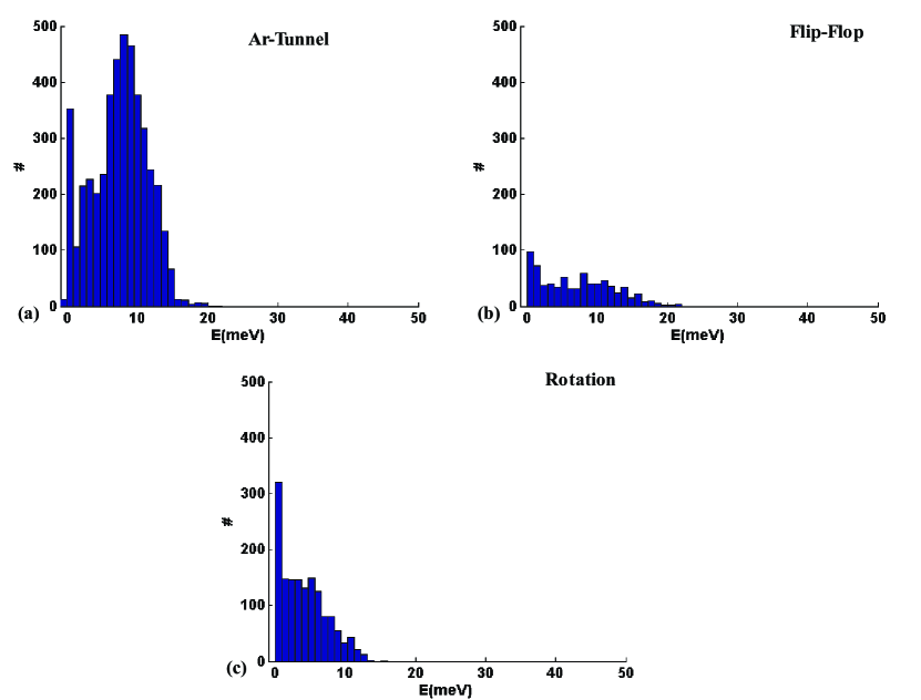
Figure 7: Histograms for TLSs up to 20% N₂ density.

On of the material properties that are of main interest and is the he coupling of the different TLSs with phonons. For a selected number of small 2D fragments, we employed the same high-quality, high-cost DFT methods presented in [3] to extract the values of the TLS-phonon interaction energy $\gamma$ of the different TLSs and also to estimate the compression energy per atom. To test the validity of the numerical approach we are performing, we construct identical lattices which we treat with our Lennard-Jones-based method and with DFT (B3LYP, 6-311G). We find that the sign of $\gamma_{S}$ obtained by Lennard-Jones is confirmed by DFT in all cases examined. While correct in sign and order of magnitude, we do find that Lennard-Jones overestimates the value of $\gamma_{S}$ by a factor of 2-4. Lennard-Jones underestimates the value of the compression energy of two neighboring Ar atoms $C$ by up to an order of magnitude compared with high-level DFT calculations. On the other hand, a smaller basis set such as 3-21G, which is still much more expensive than the method presented here, results in values that are comparable to LJ for all problems tested.

Table 1: $\gamma_{S}$(rotation) in different configurations. Problem A: 3x3 pristine Ar lattice with a central N₂. Problem B: 5x5 pristine Ar lattice with a central N₂. Problem C: 5x5 pristine Ar lattice with three nearest neighbours N₂ in the central line, oriented parallel to each other and perpendicular to the line defined by their centers, [8].

	A	B	C
$C$ (LJ,meV)	1.0	0.15	0.5
$C$ (DFT,meV)	1.8	1.6	1.7
$\gamma_{S}$ (LJ,eV)	1.44	0.60	0.96
$\gamma_{S}$ (DFT,eV)	0.60	0.320	0.22

The results in Table 1 were tested by performing extra calculations, e.g. with even larger basis sets such as 6-311+G* or in Problem D, defined as Problem C but with an extra layer resulting in a 7x7 lattice. Thus, using basis set 6-311+G* instead of 6-311G in problem A results in a $\gamma_{S}=0.56$ eV (rather than 0.60), showing that the 6-311G is already a good enough basis for this problem. The comparison of Problems C and D at LJ and DFT (3-21G) levels confirms the qualitative results presented above, both on $C$ and $\gamma_{S}$.

6 Conclusions

We have presented a technique for producing data for studying the coupling between local (TLS) and extended (phonon) interactions in disordered solids that is capable of dealing with a statistically representative number of large systems i.e. with negligible border effects. We rely on a discrete atomic model based on the well known Lennard Jones Potential, to compute and simulate the equilibrium of an atomic lattice, with randomly introduced impurities. A MC cooling is also performed to obtain more stable configurations. The results are extracted from the central region of a large lattice and thus effectively correspond to a disordered infinite medium. We applied the developed technique for an analysis of the coupling on a Ar:N₂ mixture, as it is a physically intriguing case of disordered lattice where ample experimental information is available. A discussion about the physical properties of this system which employs the presented method is performed in [8]

The non linear spring-like models have limitations in terms of accuracy and convergence in comparison with other minimization methods for discrete systems, as the conjugate gradient used in [5]. However, the notation and structure of its mathematical matrix expression is very similar to a finite element formulation, thus it simplifies the description of boundary conditions and enhances its versatility. Moreover, as its stability is very sensitive to initial conditions, in comparison with other more stable optimization methods, which allows the fast discarding of configurations which would either fail to converge or take a long time to converge, effectively reducing the computation time for producing a statistical representative dataset for TLSs analysis.

The technique, even lacking the accuracy of ab initio models or other non linear techniques as the conjugate gradient, is able to reproduce the qualitative behavior of TLSs. Furthermore, it solves some problems that do not allow the application of such more accurate methods to the study infinite disordered solids considering large samples. Besides, the methodology introduced is also suitable for its applications with other potentials, like Morse, Harmonic or coulomb electric potentials and even MC techniques for considering high temperature systems. However as the basic model is very close to the MD approach, the techniques developed for the interpretation of material properties on MD framework can also be applied in our model. Another advantage of the proposed technique is that the obtained atomic equilibrium positions can be used as starting position for other more accurate techniques. Thus the statistically representative sample obtained with our approach improves the usability range and general applicability of the conventional, more expensive techniques.

The strategy employed on the random enrichment of the lattice with impurities shows further advantages. The random introduction of impurities allows the consideration of amorphous medium but the iteratively approach helps to achieve higher impurity density in contrast with a pure random enrichment. Moreover, having several histories with different level of impurity density increases the data for the statistical analysis. besides as only the possibility with minimum energy is stored it helps to have always a ground like state, simplifying the cooling. The technique is also suitable for performing 3D TLS studies in a feasible time, however some mathematical and physical considerations have to be taken into account to enforce stability of those systems as they are more sensitive to initial conditions. All in all, we present a computational cheap technique to produce data suitable for statistical analysis for TLSs properties with advantages relying on its velocity and versatility.

The procedure presented also is suitable to study the macroscopic properties of an amorphous solid starting from its microscopic behavior: the discrete model description relies on atom positions, forces and displacements, and can be easily extended and simplifies the introduction of boundary conditions. Of course, whenever adequate the parameters of the procedure such as lattice size, distance of equilibrium, number of steps, number of considered families for the enrichment and MC steps, can be modified to achieve an improved accuracy.

References

- [1] Reinisch J, Heuer A. Local properties of the potential-energy landscape of a model glass: Understanding the low-temperature anomalies.Physical Review Letters B 2004; 70: 6421–6428.
- [2] Schechter M, Stamp PCE. Inversion symmetric two-level systems and the low-temperature universality in disordered solids. Physical Review Letters B 2013; 88(17): 174202.
- [3] Gaita-Ariño A, Schechter M. Identification of Strong and Weak Interacting Two-Level Systems in KBr:CN. Physical Review Letter 2011; 107(10): 105504
- [4] Pohl RO, Liu X, Crandall RS.Lattice vibrations of disordered solids. Current Opinion in Solid State and Materials Science 1999; 4 (3): 281–287.
- [5] Churkin A, Barash D, Schechter M. Nonhomogeneity of the density of states of tunneling two-level systems at low energies. Physical Review Letters B 2014; 89 (10): 104202
- [6] Kwon YW. Discrete atomic and smeared continuum modelling for static analysis. Engineering Computations 2003; 20(8): 964–78
- [7] Burczynski T, Mrozek A, Kuś W. A computational continuum-discrete of materials. Bulletin of the polish academy of sciences. Technical Sciences 2007; 55(1): 85–89
- [8] Gaita-Ariño A, González-Albuixech VF, Schechter M. ArN2 - a non universal glass Physical Review B Under Review. arXiv:1405.2217
- [9] Wang Y, Suna Ch, Suna X. Hinkleyb J. Odegardb GM. Gates TS.2-D nano-scale finite element analysis of a polymer field. Composites Science and Technology 2003; 63: 1581-1590
- [10] Lennard Jones LE. On the determination of molecular fields- II. From the equation of state of a gas. Proceedings of the Royal Society, Ser A 1924;106:463
- [11] Karakasidis TE, Liakopoulos AB. Two-regime dynamical behaviour in Lennard Jones systems: Spectral and rescaled range analysis. Physica A: Statistical Mechanics and its Applications 2004; 333: 225–240.
- [12] Verlet L. Computer ”Experiments” on Classical Fluids. I. Thermodynamical Properties of Lennard-Jones Molecules.Physical Reviews 1967; 159 (1): 98–103.
- [13] Verlet L. Computer ”Experiments” on Classical Fluids. II. Equilibrium Correlation Functions.Physical Reviews 1968; 165 (1): 201–214
- [14] Heyes DM. Thermal conductivity and bulk viscosity of simple fluids. A molecular-dynamics study. Journal of Chemical Society. Faraday Transactions 1984; 80 (11): 1363–1394.
- [15] Nielaba P, Binder K. Lattice Deformations in a N-Ar Mixture Model in the Diluted Limit. Europhysics Letters 1990; 13(4): 327–33
- [16] Hoover WG, Holt AC, Shortle DR, Gray SG. Comparison of Lennard-Jones and Exponential:Six Pair Potentials for Solid Argon at Low Pressure. The Journal of Chemical Physics 1970; 52, 1782–1784
- [17] Reynolds PA. Lattice dynamics of the pyrazine crystal structure by coherent inelastic neutron scattering. The Journal of Chemical Physics 1973; 59: 2777–2786
- [18] Johnson E, Hazoume RP. Application of the RISM Method to Lennard-Jones. Interaction Site Molecular Fluids The Journal of Chemical Physics 1979; 70: 1599–1601)
- [19] Romano S. Monte Carlo simulation of a two dimensional anisotropic plane rotator model. Liquid Crystals 1989; 6 (4): 457–466.
- [20] Leonel SA, Coura PZ, Pereira AR, Mól LAS, Costa BV. Monte Carlo study of the critical temperature for the planar rotator model with nonmagnetic impurities. Physical Review B 2003; 67 (10): 104426.