How nanomechanical systems can minimize dissipation

Abstract

Information processing machines at the nanoscales are unavoidably affected by thermal fluctuations. Efficient design requires understanding how nanomachines can operate at minimal energy dissipation. In this letter we focus on mechanical systems controlled by smoothly varying potential forces. We show that optimal control equations way if the energy cost to manipulate the potential is taken into account. When such cost becomes negligible, optimal control strategy can be constructed by transparent geometrical methods and recovers the solution of optimal mass transport equations in the overdamped limit. Our equations are equivalent to hierarchies of kinetic equations of a form well-known in the theory of dilute gases. From our results, optimal strategies for energy efficient nanosystems may be devised by established techniques from kinetic theory.

Recent experiments with colloidal particles, and integrated platforms of nanomagnetic memory and logic circuits exhibited the possibility to design and control information processing machines on a molecular scale Toyabe et al. (2010); Lambson, Carlton, and Bokor (2011); Bérut et al. (2012). These experiments are a first experimental step towards low dissipation Brownian computers, a concept theoretically envisaged decades ago Bennett (1982). Furthermore, these experiments put to test new developments of non-equilibrium thermodynamics such as refinements of the Second Law stemming from fluctuation theorems (see e.g. Evans and Searles (1994); Gallavotti and Cohen (1995); Jarzynski (1997); Crooks (1997); Jiang, Qian, and Qian (2004) and also Dillenschneider and Lutz (2009); Aurell et al. (2012)). Engineering nanomachines, however, remains technologically challenging Van den Broeck (2010) and demands a better theoretical understanding of how energy dissipation can be minimized.

The Langevin–Kramers dynamics is the reference model (c. f. van Kampen (2007)) epitomizing effects in nanosystem mechanics: kinetic-plus-potential Hamiltonian, mechanical friction by a Stokes drag force, and thermal noise. In the Langevin–Kramers framework, the Second Law of thermodynamics is amenable to a mathematical formulation in terms of an adapted Schrödinger diffusion problem Aebi (1996): given the phase space probability densities describing the state of the system at finite initial and final times, find the potential force which steers the initial into the final density while minimizing the average energy dissipation.

In this letter we conceptualize the Schrödinger diffusion as an optimal stochastic control problem Fleming and Soner (2006). Our aim is to derive the optimal control strategy over the class of smooth potential forces for the problem adapted to the Second Law of Thermodynamics. From the experimental slant, smooth potentials model macroscopic degrees of freedom of the system whose state is determined by external sources Alemany, Ribezzi, and Ritort (2011). We show that our problem is well-posed when regarded as the limit of a more general control problem which takes into account the energy cost of the control. The phase-space optimal control equations turn out to be amenable to the form of Bogoljubov–Born–Green–Kirkwood–Yvon kinetic momentum hierarchies, which are well-known in the theory of dilute gases (see e.g. Cercignani, Illner, and Pulvirenti (1994)). This is an important observation as it renders immediately available a toolbox of mathematical methods for the analysis of our optimal control equations Levermore (1996). In agreement with physical intuition, in the overdamped regime we recover the Monge–Ampère–Kantorovich equations Villani (2009), which were recently proved to govern minimal dissipation transitions in the Langevin–Smoluchowski modeling Aurell, Mejía-Monasterio, and Muratore-Ginanneschi (2011). Moreover, elementary arguments show that the solution of the very same Monge–Ampère–Kantorovich equations yield a general lower bound for the average energy dissipation by smooth Langevin–Kramers dynamics.

Finally, we notice that our results are based on Pontryagin’s principle (see Boscain and Piccoli (2005) for a concise review) in a formulation inspired by Guerra and Morato (1983). To the best of our knowledge, our formulation is a novelty which may be of relevance for control problems in other disciplines.

IModel

We define the kinetic-plus-potential Langevin–Kramers dynamics by means of its scalar generator

$$\mathfrak{L}=\frac{\boldsymbol{p}}{m}\cdot\partial_{\boldsymbol{q}}-\left(\frac{\boldsymbol{p}}{\tau}+\partial_{\boldsymbol{q}}U\right)\cdot\partial_{\boldsymbol{p}}+\frac{m}{\beta\,\tau}\partial_{\boldsymbol{p}}^{2}$$

Here $\beta$ is the inverse of the temperature, $m$ is the mass of a Brownian particle under a time dependent potential force $\partial_{\boldsymbol{q}}U\equiv(\partial_{\boldsymbol{q}}U)(\boldsymbol{q},t)$, and $\tau$ is the characteristic time of the Stokes drag. We suppose the dynamics to occur on an $2d$-dimensional Euclidean phase space with coordinates $\boldsymbol{x}\equiv\left[\boldsymbol{q}\,,\boldsymbol{p}\right]$, where $\boldsymbol{q}$ and $\boldsymbol{p}$ denote as usual positions and momenta. By the generator $\rho\equiv\rho\left(\boldsymbol{x},t\right)$ evolves then according to the Fokker–Planck equation

$$(\partial_{t}-\mathfrak{L}^{\dagger})\rho=0$$ (1)

where $\mathfrak{L}^{\dagger}$ is the $\mathbb{L}^{2}(\mathbb{R}^{2d})$ adjoint of $\mathfrak{L}$ with respect to the Lebesgue measure. Stochastic thermodynamics considerations (see e.g. Jiang, Qian, and Qian (2004); Chétrite and Gawȩdzki (2008)) uphold the interpretation of

$$\mathcal{Q}=-\frac{d\,t_{\mathrm{f}}}{\beta\,\tau}+\int_{0}^{t_{\mathrm{f}}}\mathrm{d}t\int_{\mathbb{R}^{2d}}\mathrm{d}^{2d}x\,\rho\frac{\|\boldsymbol{p}\|^{2}}{m\,\tau}$$

as the mean heat release by the Brownian particle during the time interval $[0,t_{\mathrm{f}}]$. The mean heat release is given by the expected value of the line integral over the Stokes drag

$$\mathcal{E}=\int_{0}^{t_{\mathrm{f}}}\mathrm{d}t\int_{\mathbb{R}^{2d}}\mathrm{d}^{2d}x\,\rho\frac{\|\boldsymbol{p}\|^{2}}{m\,\tau}$$ (2)

minus its Maxwell–Boltzmann equilibrium equipartition value. Hence, finding a tight lower bound for the Second Law of thermodynamics over finite-time transitions governed by (1) and transforming $\rho(\boldsymbol{x},0)=\rho_{\iota}(\boldsymbol{x})$ into $\rho(\boldsymbol{x},t_{\mathrm{f}})=\rho_{\mathrm{f}}(\boldsymbol{x})$ is equivalent to finding a Schrödinger diffusion process which minimizes (2) by an optimal choice of $U$. In this letter, we will always consider boundary conditions compatible with thermal equilibrium: $\rho_{\mathrm{j}}(\boldsymbol{x})=\mu_{\mathrm{j}}(\boldsymbol{q})\mu_{\scriptscriptstyle{MB}}(\boldsymbol{p})$, $\mathrm{j}=\mathrm{\iota},\mathrm{f}$ with $\mu_{\scriptscriptstyle{MB}}(\boldsymbol{p})=[\beta/(2\,\pi\,m)]^{d/2}\exp\left\{-\frac{\beta\,\|\boldsymbol{p}\|^{2}}{2\,m}\right\}$ the Maxwell–Boltzmann momentum distribution.

IIBounds

Elementary statistical moment inequalities immediately yield

$$\mathcal{E}\geq\int_{0}^{t_{\mathrm{f}}}\frac{\mathrm{d}t}{\tau}\int_{\mathbb{R}^{d}}\mathrm{d}^{d}q\,\mu\,m\,\|\boldsymbol{v}\|^{2}$$ (3)

with the marginal density $\mu(\boldsymbol{q},t)\equiv\int_{\mathbb{R}^{d}}\mathrm{d}^{d}p\,\rho(\boldsymbol{q},\boldsymbol{p},t)$ and the macroscopic velocity (or first order kinetic cumulant) $\boldsymbol{v}(\boldsymbol{q},t)\equiv[\mu(\boldsymbol{q},t)\,m]^{-1}\int_{\mathbb{R}^{d}}\mathrm{d}^{d}p\,\rho(\boldsymbol{q},\boldsymbol{p},t)\,\boldsymbol{p}$. A well-known result of kinetic theory Cercignani, Illner, and Pulvirenti (1994) implies that $\mu$ obeys a continuity equation with respect to $\boldsymbol{v}$. Hence we obtain (see e.g. Muratore-Ginanneschi (2014) and below) a lower bound for the right hand side of (3) if we choose $\boldsymbol{v}$ to be solution of a Monge–Ampère–Kantorovich system (Burgers plus mass continuity) transporting $\mu_{\iota}$ into $\mu_{\mathrm{f}}$ in $[0,t_{\mathrm{f}}]$. Repeating analogous considerations on conditional position averages yields for equilibrium boundary conditions the bound $\mathcal{Q}\,\geq\,0$. In general, there is no reason to expect these simple bounds to be tight. Moreover, the knowledge of $\boldsymbol{v}$ does not specify an optimal control $U$.

IIIOptimal Control

To tackle the optimal control problem we construct from (2) the energy cost functional

$$\mathcal{A}=\mathcal{E}+\frac{2\,g}{\beta}\mathcal{D}\left(\rho\|\bar{\rho}\right)-\int_{0}^{t_{\mathrm{f}}}\mathrm{d}t\int_{\mathbb{R}^{2d}}\mathrm{d}^{2d}x\,V\left(\partial_{t}-\mathfrak{L}^{\dagger}\right)\rho$$ (4)

where $g\geq 0$ and, upon denoting the local equilibrium potential by $S(\boldsymbol{q},t)=-\ln\frac{\tau^{d}\,\mu(\boldsymbol{q},t)}{\beta^{d/2}\,m^{d/2}}$, we define

$$\mathcal{D}\left(\rho\,\|\,\bar{\rho}\right)\equiv\frac{\tau\,\beta}{2\,m}\int_{0}^{t_{\mathrm{f}}}\mathrm{d}t\int_{\mathbb{R}^{2d}}\mathrm{d}^{2d}x\,\rho\,\|\partial_{\boldsymbol{q}}(U-\tfrac{k}{\beta}\,S)\|^{2}$$

with a real constant $k$.

The last term in (4) encapsulates Pontryagin’s principle. Namely, the term vanishes if $\rho$ satisfies the Fokker-Planck equation (1). Thus, the dynamics is enforced by the Lagrange multiplier $V\equiv V(\boldsymbol{x},t)$, which we interpret as the value function of Bellman’s formulation of optimal control Fleming and Soner (2006). The parameter $g\,\geq\,0$ couples the energy dissipation $\mathcal{E}$ to a term $\mathcal{D}$ modeling the energy cost of the control. Namely, $\mathcal{D}\left(\rho\,\|\,\bar{\rho}\right)$ is the Kullback-Leibler divergence between $\rho$ of the process and the density $\bar{\rho}$ of a Langevin–Kramers process driven by the potential $\smash{\tfrac{k}{\beta}}\,S$. As $\smash{\tfrac{1}{\beta}}\,S$ is the local equilibrium potential for the position marginal density, $\mathcal{D}\left(\rho\,\|\,\bar{\rho}\right)$ vanishes at equilibrium for $k=1$. The case $k=0$ describes instead the relative entropy between the controlled and the uncontrolled ($U=0$) Langevin–Kramers dynamics.

Following Pontryagin’s principle, we look for extremal value of the energy cost functional (4) versus the triple $(\rho,V,U)$. The calculation is straightforward but relies on three crucial observations. First, for any $g\,>\,0$, the energy cost is convex in the control $\partial_{\boldsymbol{q}}U$ and hence coercive Fleming and Soner (2006). Second, the energy cost depends non linearly upon $\rho$ via the local equilibrium potential $S$. Third, since $U$ depends only upon position variables, we can average out momenta from energy cost variations with respect to $U$. We thus arrive to the system of three extremal equations formed by: first, the Fokker-Planck equation (1); second, the dynamic programming equation

$$(\partial_{t}+\mathfrak{L})V+\frac{\parallel\boldsymbol{p}\parallel^{2}}{m\,\tau}+\frac{2\,g}{\beta}\mathcal{D}_{\rho}^{\prime}=0$$ (5)

with $\mathcal{D}_{\rho}^{\prime}\equiv\frac{\beta\,\tau}{2\,m}\,\{\|\partial_{\boldsymbol{q}}(U-\frac{k}{\beta}S)\|^{2}-\frac{2\,k}{\beta}\partial_{\boldsymbol{q}}^{2}(U-\frac{k}{\beta}S)\}$; and third, the equation for the control potential

$$\nabla_{\boldsymbol{q}}^{\scriptscriptstyle{S}}\cdot\bigl{(}\tfrac{m}{2\tau}\,\mathsf{V}^{\scriptscriptstyle{(1)}}-g\,\partial_{\boldsymbol{q}}(U-\tfrac{k}{\beta}S)\bigr{)}=0$$ (6)

where we write $\nabla_{\boldsymbol{q}}^{\scriptscriptstyle{S}}\equiv\partial_{\boldsymbol{q}}-(\partial_{\boldsymbol{q}}S)$ and define

$$\mathsf{V}^{\scriptscriptstyle{(1)}}(\boldsymbol{q},t)=\int_{\mathbb{R}^{d}}\mathrm{d}^{d}p\,\frac{\rho(\boldsymbol{q},\boldsymbol{p},t)}{\mu(\boldsymbol{q},t)}\,\partial_{\boldsymbol{p}}V(\boldsymbol{q},\boldsymbol{p},t)$$ (7)

These three equations, the optimal control system, is the first result of this letter. We now turn to analyze its main physical consequences.

IVKinetic hierarchies and controllability

In general, we can turn the energy cost (4) into an average restricted to configuration space by introducing conditional momentum cumulants of any order $n$:

$$\mathsf{F}_{\boldsymbol{i}_{n}}^{\scriptscriptstyle{(n)}}(\boldsymbol{q},t)\equiv\left.\frac{\partial_{\boldsymbol{\bar{p}}_{i_{1}}}\dots\partial_{\boldsymbol{\bar{p}}_{i_{n}}}}{m^{n}\,\imath^{n}}\ln\int_{\mathbb{R}^{d}}\mathrm{d}^{d}p\,e^{\imath\boldsymbol{\bar{p}}\cdot\boldsymbol{p}}\frac{\rho(\boldsymbol{q},\boldsymbol{p},t)}{\mu(\boldsymbol{q},t)}\right|_{\boldsymbol{\bar{p}}=0}$$

together with dual tensors $\left\{\mathsf{V}_{\boldsymbol{i}_{n}}^{\scriptscriptstyle{(n)}}\right\}_{n=0}^{\infty}$. Here we denote by $\boldsymbol{i}_{n}\equiv\,[i_{1},\dots,i_{n}]$ the $n$-tuple of Euclidean indices of any rank-$n$ cumulant or dual tensor. If we apply Pontryagin’s principle by looking for stationary variations of $\left\{\mathsf{F}_{\boldsymbol{i}_{n}}^{\scriptscriptstyle{(n)}},\mathsf{V}_{\boldsymbol{i}_{n}}^{\scriptscriptstyle{(n)}}\right\}_{n=0}^{\infty}$ and $\mu$, then instead of the Fokker–Planck equation (1) and the dynamic programming (5) we obtain two coupled hierarchies of kinetic equations for the $\mathsf{F}^{\scriptscriptstyle{(n)}}$’s and the $\mathsf{V}^{\scriptscriptstyle{(n)}}$’s and the local equilibrium potential $S$:

$$\left(\partial_{t}+\boldsymbol{v}\cdot\partial_{\boldsymbol{q}}+\frac{n}{\tau}\right)\mathsf{F}_{\boldsymbol{i}_{n}}^{\scriptscriptstyle{(n)}}+\frac{1}{m}\sum_{l=2}^{n}\binom{n}{l}\,\underset{\boldsymbol{i}_{n-l},\boldsymbol{i}_{l}}{\operatorname{Sym}}\mathsf{F}_{\boldsymbol{i}_{n-l},j}^{\scriptscriptstyle{(n-l+1)}}\partial_{\boldsymbol{q}_{j}}\mathsf{F}_{\boldsymbol{i}_{l}}^{\scriptscriptstyle{(l)}}+\frac{1}{m}\nabla_{\boldsymbol{q}_{j}}^{\scriptscriptstyle{S}}\mathsf{F}_{j,\boldsymbol{i}_{n}}^{\scriptscriptstyle{(n+1)}}=\delta_{n,0}\partial_{t}S-\delta_{n,1}\partial_{\boldsymbol{q}_{i}}U+\delta_{n,2}\frac{2\,m\,\delta_{\boldsymbol{i}_{2}}}{\beta\,\tau}$$ (8)

$$\left(\partial_{t}+\boldsymbol{v}\cdot\partial_{\boldsymbol{q}}-\frac{n}{\tau}\right)\mathsf{V}_{\boldsymbol{i}_{n}}^{\scriptscriptstyle{(n)}}-\frac{1}{m}\sum_{l\geq 2}\binom{n+l-1}{l-1}\Bigl{(}\frac{n}{l}\,\underset{i,\boldsymbol{i}_{n-1}}{\operatorname{Sym}}(\partial_{\boldsymbol{q}_{i}}\mathsf{F}_{\boldsymbol{j}_{l}}^{\scriptscriptstyle{(l)}})\mathsf{V}_{\boldsymbol{j}_{l},\boldsymbol{i}_{n-1}}^{\scriptscriptstyle{(n+l-1)}}-\nabla_{\boldsymbol{q}_{j}}^{\scriptscriptstyle{S}}\mathsf{F}_{j,\boldsymbol{j}_{l-1}}^{\scriptscriptstyle{(l)}}\mathsf{V}_{\boldsymbol{j}_{l-1},\boldsymbol{i}_{n}}^{\scriptscriptstyle{(n+l-1)}}\Bigr{)}$$

$$+\frac{1}{m}\underset{i,\boldsymbol{i}_{n-1}}{\operatorname{Sym}}\bigl{(}\partial_{\boldsymbol{q}_{i}}\mathsf{V}_{\boldsymbol{i}_{n-1}}^{\scriptscriptstyle{(n-1)}}-n\,(\partial_{\boldsymbol{q}_{i}}\boldsymbol{v}_{j})\mathsf{V}_{j,\boldsymbol{i}_{n-1}}^{\scriptscriptstyle{(n)}}\bigr{)}=-\frac{\delta_{\boldsymbol{i}_{2}}\,\delta_{n,2}}{\beta\,m\,\tau}-\frac{2\,\boldsymbol{v}_{i}\,\delta_{n,1}}{\beta\,\tau}-\delta_{n,0}\biggl{(}\frac{\mathsf{F}_{j,j}^{\scriptscriptstyle{(2)}}}{m\,\tau}+\frac{m\|\boldsymbol{v}\|^{2}}{\tau}+\frac{2\,g\mathcal{D}_{\rho}^{\prime}}{\beta}\biggr{)}$$ (9)

In (8) and (9) we use the conventions that repeated (multi-)indices are contracted and that “$\operatorname{Sym}$” denotes symmetrization of the free indices in underscript. A straightforward calculation, which will be reported elsewhere, also shows that (8), (9) can be also derived directly from (1), (5). Finally, the hierarchies are coupled by (6) which continues to hold with the interpretation of a constraint relating the dual tensor $\mathsf{V}^{\scriptscriptstyle{(1)}}$ to the control potential.
The advantage of introducing (8), (9) is that we can use them to approximate the solution of our optimal control problem by means of realizable closures, i. e., finite order truncations of the hierarchies preserving the probabilistic interpretation of the cumulants Levermore (1996). We notice that truncating (8), (9) at any finite order $n$ yields a controllable system of equations in the sense that the number time derivatives in the hierarchies equals that of boundary conditions for $S$ and $\left\{\mathsf{F}^{\scriptscriptstyle{(l)}}\right\}_{l=1}^{n}$. Furthermore, increasing the order of truncation imposes more constraints on the control strategy. The solution of a sequence of realizable truncations therefore yields more and more refined lower bounds to the energy cost (4). For instance, the estimate (3) corresponds to the truncation of lowest order.

VLimit of vanishing $g$

If we set a-priori $g=0$, by Pontryagin’s principle we need to replace (6) with

$$U_{\star}(\boldsymbol{q},t)=\underset{U}{\operatorname{arg}\inf}\left\{-\int_{\mathbb{R}^{d}}\mathrm{d}^{d}q\,\mu\,\mathsf{V}^{\scriptscriptstyle{(1)}}\cdot\partial_{\boldsymbol{q}}U\right\}$$

reminiscent of singular optimal control Fleming and Soner (2006). Qualitatively, this equation suggests the decomposition of phase space into a “no-action region” where $\mathsf{V}^{\scriptscriptstyle{(1)}}$ vanishes and a “push region” where $\mathsf{V}^{\scriptscriptstyle{(1)}}\cdot\partial_{\boldsymbol{q}}U\,>\,0$ and where $\|\partial_{\boldsymbol{q}}U\|$ is constrained only by the boundary conditions. Inspecting (8), (9) shows, however, that requiring the condition $\mathsf{V}^{\scriptscriptstyle{(1)}}=0$ to hold and be preserved by the dynamics enslaves the macroscopic velocity to the remaining cumulants by the equation

$$\frac{2\boldsymbol{v}_{i}}{\tau}=\sum_{l\geq 2}\frac{(\partial_{\boldsymbol{q}_{i}}\mathsf{F}_{\boldsymbol{j}_{l}}^{\scriptscriptstyle{(l)}})\mathsf{V}_{\boldsymbol{j}_{l}}^{\scriptscriptstyle{(l)}}-l\,\nabla_{\boldsymbol{q}_{j}}^{S}\mathsf{F}_{j,\boldsymbol{j}_{l-1}}^{\scriptscriptstyle{(l)}}\mathsf{V}_{\boldsymbol{j}_{l-1},i}^{\scriptscriptstyle{(l)}}}{m}-\frac{\partial_{\boldsymbol{q}_{i}}\mathsf{V}^{\scriptscriptstyle{(0)}}}{m}$$ (10)

As the boundary values of the dual tensors $\left\{\mathsf{V}_{\boldsymbol{i}_{n}}^{\scriptscriptstyle{(n)}}\right\}_{n\neq 1}$ are determined by the boundary conditions imposed on $\mu$ and $\left\{\mathsf{F}_{\boldsymbol{i}_{n}}^{\scriptscriptstyle{(n)}}\right\}_{n\geq 2}$, we see that in general (10) cannot satisfy independent boundary conditions on $\boldsymbol{v}$. In this sense, for $g=0$ the system is not controllable. The consideration of an exactly solvable case indicates, however, that in a weaker sense $\mathsf{V}^{\scriptscriptstyle{(1)}}=0$ still governs the optimal control strategy at $g=0$.

VIEvolution between Gaussian states

Let us consider transition between Gaussian densities at finite initial and final times. Physically this is a stylized model of a moving laser trap of changing size (see Gomez-Marin, Schmiedl, and Seifert (2008) and references therein). For these boundary conditions and fixed $g>0$, the optimal control equations admit a solution in terms of a probability density which stays Gaussian in the entire control horizon, a value function which is a quadratic polynomial in $\boldsymbol{p}$ and $\boldsymbol{q}$, and a potential which is quadratic in $\boldsymbol{q}$. Correspondingly, the hierarchies (8) and (9) reduce to a system of $2d\,(2d+3)$ first order differential equations accompanied by the same number of boundary conditions for the initial and final cumulants. For dimension $d=1$ the typical behavior of the solution is shown in Figure 1 and 2 for different values of $g$.

Figure 1: (Color online) Means for Gaussian boundary conditions with parameters $\tau=1$, $m=1$, $\beta=1$, $t_{\mathrm{f}}=1$, $k=1$. The initial and final means of $\boldsymbol{x}\equiv\left[\boldsymbol{q}\,,\boldsymbol{p}\right]$ are $(0,0)$ and $(\sqrt{2},0)$, resp. The parameter $g$ varies logarithmically from $1.28\cdot 10^{-1}$ (green/light) to $1.25\cdot 10^{-4}$ (blue/dark). The arrows indicate the behavior for decreasing $g$.

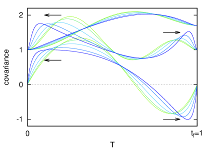
Figure 2: (Color online) Covariances for Gaussian boundary conditions with parameters as in Figure 1. The initial and final covariance matrices of $\boldsymbol{x}\equiv\left[\boldsymbol{q}\,,\boldsymbol{p}\right]$ are given by $\begin{pmatrix}1&0\\ 0&1\end{pmatrix}$ and $\begin{pmatrix}1.7&0\\ 0&1\end{pmatrix}$, resp.

As $g\to 0$ the limit behavior of the cumulants is described by the “slow manifold” specified by the condition $\mathsf{V}^{\scriptscriptstyle{(1)}}=0$ and the evolution law (10). Only in a layer close to the boundaries of the control horizon cumulants get away from the slow manifold along exponentially stable and unstable directions with rates of the order $O(1/\sqrt{g})$ in order to satisfy the boundary conditions. The description of singular boundary value problems in terms of invariant manifolds is well known in the theory of dynamical systems Tin, Kopell, and Jones (1994). We refer the interested reader to PMG for the details of the multiscale expansion Pavliotis and Stuart (2008) proving the foregoing qualitative picture.

VIIOverdamped limit

The relevance of the “slow manifold” condition $\mathsf{V}^{\scriptscriptstyle(1)}=0$ appears from the fact that it permits to recover directly at $g=0$ the “overdamped” limit of the Langevin–Kramers dynamics. The overdamped regime corresponds to the assumption of a wide scale separation between the control horizon $[0,t_{\mathrm{f}}]$ and the Stokes time $\tau$ and between the characteristic length scale $L$ of the configuration space boundary data $\mu_{\mathrm{\iota}}(\boldsymbol{q}/L)$, $\mu_{\mathrm{f}}(\boldsymbol{q}/L)$ and the typical length scale $\ell=\tau/\sqrt{\beta\,m}$ of the uncontrolled process. In the overdamped regime, the quantifier of the scale separation is the Stokes number $\varepsilon=\tau/t_{\mathrm{f}}=\ell^{2}/L^{2}\ll\,1$. Under these hypotheses, we can look for an asymptotic solution of (1) and (5) by expanding around a Maxwell–Boltzmann momentum equilibrium distribution $\mu_{\scriptscriptstyle{MB}}(\boldsymbol{p})$ perturbed at large scales, $(\boldsymbol{\tilde{q}},\tilde{t})\equiv(\sqrt{\varepsilon}\,\boldsymbol{q},\varepsilon t)$, by the action of a control potential of the form $U(\boldsymbol{q},t)\equiv U_{0}(\sqrt{\varepsilon}\,\boldsymbol{q},\varepsilon t)+O\left(\sqrt{\varepsilon}\right)$. From now on we specify by an underscript the order of the perturbative expansion. Upon setting $\partial_{\boldsymbol{\tilde{q}}}S_{0}=-\partial_{\boldsymbol{\tilde{q}}}\ln\mu_{0}$, and applying standard homogenization techniques (see e.g. Pavliotis and Stuart (2008), see also Muratore-Ginanneschi (2014)) we get for the solution of the Fokker–Planck equation (1):

$$\rho(\boldsymbol{p},\boldsymbol{\tilde{q}},\tilde{t})=\mu_{\scriptscriptstyle{MB}}(\boldsymbol{p})\,\mu_{0}(\boldsymbol{\tilde{q}},\tilde{t})\times$$

$$\Bigl{(}1+\sqrt{\varepsilon}\,\tfrac{\tau}{m}\,\boldsymbol{p}\cdot\partial_{\boldsymbol{\tilde{q}}}(S_{0}-\beta\,U_{0})(\boldsymbol{\tilde{q}},\tilde{t})+O(\varepsilon)\Bigr{)}$$ (11)

For the solution of the dynamic programming (5) we obtain

$$V(\boldsymbol{p},\boldsymbol{\tilde{q}},t,\tilde{t})=\frac{(t_{\mathrm{f}}-t)\,d}{\beta\,\tau}+\frac{\|\boldsymbol{p}\|^{2}}{2\,m}+V_{0}(\boldsymbol{\tilde{q}},\tilde{t})+$$

$$\sqrt{\varepsilon}\Bigl{(}V_{1}(\boldsymbol{\tilde{q}},\tilde{t})+\tfrac{\tau}{m}\,\boldsymbol{p}\cdot\partial_{\boldsymbol{\tilde{q}}}\,(V_{0}-U_{0})(\boldsymbol{\tilde{q}},\tilde{t})\Bigr{)}+O(\varepsilon)$$ (12)

The functions $S_{0}$ in (VII) and $V_{0}$ in (VII), respectively, obey the local equilibrium potential equation

$$\partial_{\tilde{t}}S_{0}-\tfrac{\tau}{m}\Bigl{(}(\partial_{\boldsymbol{\tilde{q}}}S_{0})\cdot\partial_{\boldsymbol{\tilde{q}}}-\partial_{\boldsymbol{\tilde{q}}}^{2}\Bigr{)}(U_{0}-\tfrac{1}{\beta}S_{0})=0$$

and the dynamic programming equation

$$\partial_{\tilde{t}}V_{0}-\tfrac{\tau}{m}\Bigl{(}(\partial_{\boldsymbol{\tilde{q}}}U_{0})\cdot\partial_{\boldsymbol{\tilde{q}}}-\tfrac{1}{\beta}\partial_{\boldsymbol{\tilde{q}}}^{2}\Bigr{)}(V_{0}-U_{0})=0$$

These equations specifying two of the three optimal control equations governing the minimal heat release by a Langevin–Smoluchowski dynamics between $\mu_{\iota}$ and $\mu_{\mathrm{f}}$ Aurell, Mejía-Monasterio, and Muratore-Ginanneschi (2011). In order to recover the third condition, we use (VII) and (VII) to evaluate

$$\mathsf{V}^{\scriptscriptstyle{(1)}}(\boldsymbol{\tilde{q}},\tilde{t})=-\sqrt{\varepsilon}\,\tfrac{\tau}{m}\,\partial_{\boldsymbol{\tilde{q}}}\Bigl{(}2\,U_{0}-\frac{S_{0}}{\beta}-V_{0}\Bigr{)}(\boldsymbol{\tilde{q}},\tilde{t})+O(\varepsilon)$$

Then the condition $\mathsf{V}^{\scriptscriptstyle{(1)}}=0$ yields exactly the relation between $U_{0}$, $V_{0}$, $S_{0}$ that allows us to recover the very same Monge–Ampère–Kantorovich equations of Aurell, Mejía-Monasterio, and Muratore-Ginanneschi (2011):

$$\partial_{\tilde{t}}\tilde{U}-\tfrac{\tau}{2\,m}\partial_{\boldsymbol{\tilde{q}}}\tilde{U}\cdot\partial_{\boldsymbol{\tilde{q}}}\,\tilde{U}$$

$$\partial_{\tilde{t}}S_{0}-\tfrac{\tau}{m}(\partial_{\boldsymbol{\tilde{q}}}S_{0})\cdot\partial_{\boldsymbol{\tilde{q}}}\tilde{U}+\tfrac{\tau}{m}\partial_{\boldsymbol{\tilde{q}}}^{2}\tilde{U}=0$$

with $\tilde{U}\equiv U_{0}-S_{0}/\beta$.

VIIIConclusion

We showed how Pontryagin’s principle can be used to derive refined bounds for the Second Law of thermodynamics in the case of nanomechanical systems. We also established a relation between optimal control and kinetic theory, which renders available ideas and tools of dilute gas Cercignani, Illner, and Pulvirenti (1994); Levermore (1996) and optimal transport theory Villani (2009) to the construction of optimal protocols implementing at the nano-scale information processing operations such as the erasure of a bit Dillenschneider and Lutz (2009).

The authors acknowledge the Finnish Academy Center of Excellence “Analysis and Dynamics” for support. The authors are grateful to Carlos Mejía-Monasterio and Antti Kupiainen for helpful comments.

References

- Toyabe et al. (2010) S. Toyabe, T. Sagawa, M. Ueda, E. Muneyuki, and M. Sano, Nature Physics 6, 988 (2010), arXiv:1009.5287 [cond-mat.stat-mech] .
- Lambson, Carlton, and Bokor (2011) B. Lambson, D. Carlton, and J. Bokor, Physical Review Letters 107, 010604 (2011).
- Bérut et al. (2012) A. Bérut, A. Arakelyan, A. Petrosyan, S. Ciliberto, R. Dillenschneider, and E. Lutz, Nature 483, 187–189 (2012).
- Bennett (1982) C. H. Bennett, International Journal of Theoretical Physics 21, 905 (1982).
- Evans and Searles (1994) D. J. Evans and D. J. Searles, Physical Review E 50, 1645 (1994).
- Gallavotti and Cohen (1995) G. Gallavotti and E. G. D. Cohen, Physical Review Letters 74, 2694 (1995), arXiv:chao-dyn/9410007 [nlin.CD] .
- Jarzynski (1997) C. Jarzynski, Physical Review Letters 78, 2690 (1997), arXiv:cond-mat/9610209 [cond-mat.stat-mech] .
- Crooks (1997) G. E. Crooks, Journal of Statistical Physics 90, 1481 (1997).
- Jiang, Qian, and Qian (2004) D.-Q. Jiang, M. Qian, and M.-P. Qian, Mathematical Theory of Nonequilibrium Steady States, Lecture Notes in Mathematics, Vol. 1833 (Springer, 2004) p. 276.
- Dillenschneider and Lutz (2009) R. Dillenschneider and E. Lutz, Physical Review Letters 102, 210601 (2009), arXiv:0811.4351 [cond-mat.stat-mech] .
- Aurell et al. (2012) E. Aurell, K. Gawȩdzki, C. Mejía-Monasterio, R. Mohayaee, and P. Muratore-Ginanneschi, Journal of Statistical Physics 147, 487 (2012), arXiv:1201.3207 [cond-mat.stat-mech] .
- Van den Broeck (2010) C. Van den Broeck, Nature Physics 6, 937 (2010).
- van Kampen (2007) N. G. van Kampen, Stochastic processes in physics and chemistry, 3rd ed., North-Holland personal library (Elsevier, 2007) p. 463.
- Aebi (1996) R. Aebi, Schrödinger Diffusion Processes, Probability and its applications (Birkhäuser, 1996) p. 186.
- Fleming and Soner (2006) W. H. Fleming and M. H. Soner, Controlled Markov processes and viscosity solutions, 2nd ed., Stochastic modelling and applied probability, Vol. 25 (Springer, 2006) p. 428.
- Alemany, Ribezzi, and Ritort (2011) A. Alemany, M. Ribezzi, and F. Ritort, AIP Conference Proceedings 1332, 96 (2011), arXiv:1101.3174 [cond-mat.stat-mech] .
- Cercignani, Illner, and Pulvirenti (1994) C. Cercignani, R. Illner, and M. Pulvirenti, The Mathematical Theory of Dilute Gases, Applied Mathematical Sciences, Vol. 106 (Springer New York, 1994) p. 349.
- Levermore (1996) C. D. Levermore, Journal of Statistical Physics 83, 1021–1065 (1996).
- Villani (2009) C. Villani, Optimal transport: old and new, Grundlehren der mathematischen Wissenschaften, Vol. 338 (Springer, 2009) p. 973.
- Aurell, Mejía-Monasterio, and Muratore-Ginanneschi (2011) E. Aurell, C. Mejía-Monasterio, and P. Muratore-Ginanneschi, Physical Review Letters 106, 250601 (2011), arXiv:1012.2037 [cond-mat.stat-mech] .
- Boscain and Piccoli (2005) U. Boscain and B. Piccoli, in Controle non lineaire et applications, Le cours du CIMPA, edited by T. Sari (Hermann, 2005) pp. 19–66.
- Guerra and Morato (1983) F. Guerra and L. M. Morato, Physical Review D 27, 1774 (1983).
- Chétrite and Gawȩdzki (2008) R. Chétrite and K. Gawȩdzki, Communications in Mathematical Physics 282, 469 (2008), arXiv:0707.2725 [math-ph] .
- Muratore-Ginanneschi (2014) P. Muratore-Ginanneschi, Journal of Statistical Mechanics: Theory and Experiment 2014, P05013 (2014), arXiv:1401.3394 [cond-mat.stat-mech] .
- Gomez-Marin, Schmiedl, and Seifert (2008) A. Gomez-Marin, T. Schmiedl, and U. Seifert, The Journal of Chemical Physics 129, 024114 (2008), arXiv:0803.0269 [cond-mat.stat-mech] .
- Tin, Kopell, and Jones (1994) S.-K. Tin, N. Kopell, and C. K. R. T. Jones, SIAM Journal on Numerical Analysis 31, 1558 (1994).
- (27) See Supplemental Material at [URL will be inserted by publisher] for the explicit treatment of the cumulant expansion of the Gaussian model in the limit of vanishing .
- Pavliotis and Stuart (2008) G. A. Pavliotis and A. M. Stuart, Multiscale methods: averaging and homogenization, Texts in applied mathematics, Vol. 53 (Springer, 2008) p. 307.