Investigation of ⁹Be from nonlocalized clustering concept

Abstract

The nonlocalized aspect of clustering, which is a new concept for self-conjugate nuclei, is extended for the investigation of the $N\not=Z$ nucleus ⁹Be. A modified version of the THSR (Tohsaki-Horiuchi-Schuck-Röpke) wave function is introduced with a new phase factor. It is found that the constructed negative-parity THSR wave function is very suitable for describing the cluster states of ⁹Be. Namely the nonlocalized clustering is shown to prevail in ⁹Be. The calculated binding energy and radius of ⁹Be are consistent with calculations in other models and with experimental values. The squared overlaps between the single THSR wave function and the Brink+GCM (Generator Coordinate Method) wave function for the $3/2^{-}$ rotational band of ⁹Be are found to be near 96%. Furthermore, by showing the density distribution of the ground state of ⁹Be, the $\pi$-orbit structure is naturally reproduced by using this THSR wave function.

I Introduction

The clustering phenomena is one of the fundamental problems in nuclear physics. Despite of its long history since the discovery of the $\alpha$-cluster, the clustering structure in nuclei is still under active investigation Tohsaki2001 ; Funaki2002 ; Yamada2005 ; Zhou2013 ; Xu2006 ; Yren2012 . To describe the $\alpha$-cluster condensation in self-conjugate nuclei ¹²C and ¹⁶O, the Tohsaki-Horiuchi-Schuck-Röpke (THSR) wave function was proposed and provided a successful treatment of the famous Hoyle ($0_{2}^{+}$) state in ¹²C Tohsaki2001 ; Yamada2005 . The THSR wave function has been applied to different aggregates of $\alpha$-clusters including ⁸Be, ¹²C and ¹⁶O Funaki2002 ; Tohsaki2001 . It is also extended to study systems composed of general clusters such as ²⁰Ne treated as a combination of an $\alpha$-cluster and ¹⁶O Zhou2012 ; Zhou2013 . In the study of inversion-doublet-band states of ²⁰Ne, the THSR wave function, which was originally introduced to describe gas-like states, was shown to be also very suitable for the study of non gas-like cluster type of states.

The importance of the THSR wave function lies in the fact that the RGM/GCM (Resonating Group Method/Generator Coordinate Method) wave functions of both gas-like and non-gaslike states are almost 100% equivalent to single THSR wave functions. Therefore the single THSR wave function grasps the physical properties of the state. The most important property is the nonlocalized character of clustering Zhou2013 . On the other hand, superposing many Brink wave functions in the GCM approach describes non-localized clustering because the Brink-GCM wave function is almost 100% equivalent to a single THSR wave function.

Following the success in describing self-conjugate nuclei, a natural question is whether we can apply the THSR wave function to general nuclei which consist not only of $\alpha$-clusters but have also extra nucleons, such as ¹³C studied with the interaction of $\alpha$-condensation and an extra neutron Tohsaki2008 . Therefore, it would be promising to extend the THSR wave function to $N\not=Z$ nuclei.

The nucleus ⁹Be is a typical $N\not=Z$ nucleus with both $\alpha+\alpha+n$ cluster structure and also nuclear molecular orbits, which is most suitable for the extension of the THSR wave function. This study also belongs to our project which tries to understand any clustering phenomena from our new point of view. The nucleus ⁹Be has been studied with the antisymmetrized molecular dynamics free from cluster assumptions Enyo1995 . It is also investigated with the nuclear molecular orbit (MO) model in which the extra neutron occupies nuclear molecular orbits Okabe1977 ; Oertzen1996 ; Itagaki2000 . In the nuclear molecular orbit model, the wave function of the extra neutron is assumed to be a linear combination of cluster orbitals and provides a successful description of ⁹Be. However, the dynamics of the clusters is not explicitly given in these calculations. To have a clear view of the nonlocalized clustering dynamics in the ⁹Be nucleus, we need a new wave function in which this characteristic is intrinsically included. In the present work, ⁹Be is investigated with a new picture in which two $\alpha$-clusters and an extra nucleon are performing nonlocalized motion. A modified version of the THSR wave function is proposed for the description of this structure.

The outline of this paper is as follows. In Section II we formulate the THSR wave function with intrinsic parity for ⁹Be. Then in Section III we give the results of the calculation for $3/2^{-}$ rotational band of ⁹Be and analyze the structure of the ground state obtained from the THSR wave function. The last Section IV contains the conclusions.

II Formulation of THSR Wave Function for ⁹Be

The THSR wave function of ⁹Be is constructed with creation operators as

$$\left|\Phi\right\rangle=(C_{\alpha}^{\dagger})^{2}c_{n}^{\dagger}\left|{\bf\rm vac}\right\rangle,$$ (1)

where $C_{\alpha}^{\dagger}$ and $c_{n}^{\dagger}$ are creation operators of $\alpha$-particle and neutron, respectively. Here we take the same $\alpha$-creator $C_{\alpha}^{\dagger}$ as used in previous deformed THSR wave functions Funaki2002 ,

$$\begin{split}C_{\alpha}^{\dagger}=\int&d\mathbf{R}\exp(-\frac{R_{x}^{2}}{\beta_{\alpha,xy}^{2}}-\frac{R_{y}^{2}}{\beta_{\alpha,xy}^{2}}-\frac{R_{z}^{2}}{\beta_{\alpha,z}^{2}})\int d^{3}\mathbf{r}_{1}\cdots d^{3}\mathbf{r}_{4}\\ &\times\psi(\mathbf{r}_{1}-\mathbf{R})a_{\sigma_{1},\tau_{1}}^{\dagger}(\mathbf{r}_{1})\cdots\psi(\mathbf{r}_{4}-\mathbf{R})a_{\sigma_{4},\tau_{4}}^{\dagger}(\mathbf{r}_{4}),\end{split}$$ (2)

where $\mathbf{R}$ is the generate coordinate of the $\alpha$-cluster, $\mathbf{r}_{i}$ is the position of the $i$th nucleon, and the $a_{\sigma,\tau}^{\dagger}(\mathbf{r}_{i})$ is the creation operator of the $i$th nucleon with spin $\sigma$ and isospin $\tau$ at position $\mathbf{r}_{i}$. $\psi(\mathbf{r})=(\pi b^{2})^{-3/4}\exp(-r^{2}/2b^{2})$ is the single-nucleon harmonic oscillator shell model wave function representing one of the four nucleons forming the alpha cluster, where $b$ is a size parameter. $\beta_{\alpha,xy}$ and $\beta_{\alpha,z}$ are parameters for the nonlocalized motion of two $\alpha$-clusters. The subsystem of two $\alpha$-clusters is supposed to have rotational symmetry around the $z$-axis, so the same size parameters $\beta_{\alpha,xy}$ are used in $x$ and $y$ direction. For the extra neutron, we use a creation operator $c_{n}^{\dagger}$ which is similar to $C_{\alpha}^{\dagger}$ but has a new introduced phase factor,

$$\begin{split}c_{n}^{\dagger}=\int&d^{3}\mathbf{R}_{n}\exp(-\frac{R_{n,x}^{2}}{\beta_{n,xy}^{2}}-\frac{R_{n,y}^{2}}{\beta_{n,xy}^{2}}-\frac{R_{n,z}^{2}}{\beta_{n,z}^{2}})e^{im\phi_{\mathbf{R}_{n}}}\int d^{3}\mathbf{r}_{n}\\ &\times(\pi b^{2})^{-3/4}e^{-\frac{(\mathbf{r}_{n}-\mathbf{R}_{n})^{2}}{2b^{2}}}a_{\uparrow,n}^{\dagger}(\mathbf{r}_{n}),\end{split}$$ (3)

where $\mathbf{R}_{n}$ is the generate coordinate of the extra neutron, $\mathbf{r}_{n}$ is the position of the extra neutron, $a_{\sigma,\tau}^{\dagger}(\mathbf{r}_{n})$ is the creation operator of the extra neutron with spin up at position $\mathbf{r}_{n}$, and $\phi_{\mathbf{R}_{n}}$ is the azimuthal angle in spherical coordinates $(R_{\mathbf{R}_{n}},\theta_{\mathbf{R}_{n}},\phi_{\mathbf{R}_{n}})$ of $\mathbf{R}_{n}$. In this creation operator, the same size parameter $b$ of Gaussian is used as in Eq. (2). $\beta_{n,xy}$ and $\beta_{n,z}$ are parameters for the nonlocalized motion of the extra neutron.

To illustrate the detailed structure of our wave function and prove its negative parity, we can rewrite the THSR wave function of ⁹Be with $m=\pm 1$ in the form of,

$$\langle\mathbf{r}_{1},\sigma_{1},\tau_{1},\dots,\mathbf{r}_{n},\sigma_{n},\tau_{n}\left|\Phi\right\rangle\propto\mathcal{A}\left[F(\mathbf{X}_{1},\mathbf{X}_{2},\mathbf{r}_{n})\phi(\alpha_{1})\phi(\alpha_{2})\right]$$ (4)

where $\mathcal{A}$ is an antisymmetrizer, $\phi(\alpha_{1})$ and $\phi(\alpha_{2})$ are internal $\alpha$ wave functions as in Ref. Tohsaki2001 , $\mathbf{X}_{1}$ and $\mathbf{X}_{2}$ are center of mass coordinates of the two $\alpha$-clusters, and the form of function $F(\mathbf{X}_{1},\mathbf{X}_{2},\mathbf{r}_{n})$ is,

$$\begin{split}F(\mathbf{X}_{1},\mathbf{X}_{2},\mathbf{r}_{n})=&\exp\left\{-\frac{X_{1,x}^{2}+X_{1,y}^{2}+X_{2,x}^{2}+X_{2,y}^{2}}{C_{\alpha,xy}^{2}}-\frac{X_{1,z}^{2}+X_{2,z}^{2}}{C_{\alpha,z}^{2}}\right\}\\ &\times\exp\left\{-\frac{r_{n,x}^{2}+r_{n,y}^{2}}{C_{n,xy}^{2}}-\frac{r_{n,z}^{2}}{C_{n,z}^{2}}\right\}\\ &\times[I_{0}(\frac{r_{n,x}^{2}+r_{n,y}^{2}}{A^{2}})+I_{1}(\frac{r_{n,x}^{2}+r_{n,y}^{2}}{A^{2}})]\\ &\times(r_{n,x}^{2}+r_{n,y}^{2})^{1/2}e^{\pm i\phi_{r_{n}}}\end{split}$$ (5)

where $I_{0}$ and $I_{1}$ are the modified Bessel functions of the first kind, $\phi_{r_{n}}$ is the azimuthal angle of $\mathbf{r}_{n}$, and the denominators are, $C_{\alpha,xy}^{2}=b^{2}/2+\beta_{\alpha,xy}^{2}$,  $C_{\alpha,z}^{2}=b^{2}/2+\beta_{\alpha,z}^{2}$,   $C_{n,xy}^{2}=(8b^{4}+4b^{2}\beta_{n,xy}^{2})/(4b^{2}+\beta_{n,xy}^{2})$,  $C_{n,z}^{2}=2b^{2}+\beta_{n,z}^{2}$,  and  $A^{2}=4b^{2}+8b^{4}/\beta_{n,xy}^{2}$. The detailed derivation of Eq. (4) and Eq. (5) can be found in the appendix.

The wave function in Eq. (4) gives a clear view of the dynamics of motions inside nucleus ⁹Be as a single function without superposition. It consists of two parts, the internal motion of nucleons inside $\alpha$-clusters $\phi(\alpha_{1})$ and $\phi(\alpha_{2})$, and the center-of-mass motions of clusters and the extra neutron described by $F(\mathbf{X}_{1},\mathbf{X}_{2},\mathbf{r}_{n})$. The negative parity of our THSR wave function with $m=\pm 1$ can be clearly obtained with Eq. (4) and Eq. (5). The Gaussians and the modified Bessel functions in function $F$ will not change under the inversion of space. For the last phase factor $e^{i\phi_{r_{n}}}$ in function $F$, we have ${\hat{P}}_{r}e^{\pm i\phi_{r_{n}}}=e^{\pm i(\pi+\phi_{r_{n}})}=-e^{\pm i\phi_{r_{n}}}$, which results in a negative parity for the function $F(\mathbf{X}_{1},\mathbf{X}_{2},\mathbf{r}_{n})$. Considering that internal wave functions $\phi(\alpha_{1})$ and $\phi(\alpha_{2})$ have positive parity, thus the negative parity of the THSR wave function with $m=\pm 1$ is demonstrated.

We give another proof of the negative parity of our ⁹Be wave function without executing the integrations over $\mathbf{R}$ and $\mathbf{R}_{n}$: The spatial wave function of the extra neutron $\Phi_{n}(\mathbf{r}_{n})$ can be written as,

$$\begin{split}\Phi_{n}(\mathbf{r}_{n})=\int&d^{3}\mathbf{R}_{n}\exp(-\frac{R_{n,x}^{2}}{\beta_{n,xy}^{2}}-\frac{R_{n,y}^{2}}{\beta_{n,xy}^{2}}-\frac{R_{n,z}^{2}}{\beta_{n,z}^{2}})e^{im\phi_{\mathbf{R}_{n}}}\\ &\times(\pi b^{2})^{-3/4}e^{-\frac{(\mathbf{r}_{n}-\mathbf{R}_{n})^{2}}{2b^{2}}}.\end{split}$$ (6)

When we change the integration variables $(R_{n,x},R_{n,y},R_{n,z})$ to $(-R_{n,x},-R_{n,y},-R_{n,z})$, in the integral representation of $\Phi_{n}(-r_{n})$ by Eq. (6), we obtain $\Phi_{n}(-r_{n})=-\Phi_{n}(r_{n})$. It is because the azimuthal angle of $(-R_{n,x},-R_{n,y},-R_{n,z})$ is $(\pi+\phi_{\mathbf{R}_{n}})$ and $\exp(i(\pi+\phi_{\mathbf{R}_{n}}))=-\exp(i\phi_{\mathbf{R}_{n}})$. When $m=0$, Eq. (6) is a standard THSR wave function and has a positive parity as already known before in Ref. Zhou2013 . So the total parity of ⁹Be is now determined by $m$,

$$\pi=\pi_{\alpha}^{(1)}\times\pi_{\alpha}^{(2)}\times\pi_{n}=\begin{cases}+&(m=0)\\ -&(m=\pm 1).\end{cases}$$ (7)

From Eq. (5) we can also see that the $z$ component of orbital angular momentum $l_{z,n}=m$ is a good quantum number for the extra neutron. Because of the rotational symmetry of the two-$\alpha$-cluster subsystem about $z$-axis, we have $l_{z,\alpha}=0$ for $\alpha$ clusters. Thus the $z$-component of the orbital angular momentum $l_{z}$ of total system is

$$l_{z}=l_{z,\alpha}^{(1)}+l_{z,\alpha}^{(2)}+l_{z,n}=m.$$ (8)

In order to eliminate effects from spurious center-of-mass (c.o.m.) motion, the c.o.m. part of $\left|\Phi\right\rangle$ is projected onto a $(0s)$ state Okabe1977 ,

$$\left|\Psi\right\rangle=\left|(0s)\text{c.o.m.}\right\rangle\rangle\left\langle\langle(0s)\text{c.o.m.}|\Phi\right\rangle.$$ (9)

Here $(0s)$ represents the wave function of the c.o.m. coordinate $\mathbf{X}_{G}$, which is the ground state of harmonic oscillator. For the THSR wave function of ⁹Be, this projection can be accomplished simply by the transformation of coordinates $\mathbf{r}_{i}$ in $\left|\Phi\right\rangle$ as

$$\mathbf{r}_{i}\rightarrow\mathbf{r}_{i}-\mathbf{X}_{G}.$$ (10)

Then the spurious center-of-mass motion in the wave function can be separated and eliminated analytically.

We also apply the angular-momentum projection technique $\hat{P}_{MK}^{J}\left|\Psi\right\rangle$ to restore the rotational symmetry Schuck1980 ,

$$\begin{split}\left|\Psi^{JM}\right\rangle&=\hat{P}_{MK}^{J}\left|\Psi\right\rangle\\ &=\frac{2J+1}{8\pi^{2}}\int d\Omega D^{J*}_{MK}(\Omega)\hat{R}(\Omega)\left|\Psi\right\rangle,\end{split}$$ (11)

where $J$ is the total angular momentum of ⁹Be.

The Hamiltonian of ⁹Be system can be written as

$$H=\sum_{i=1}^{9}T_{i}-T_{c.m.}+\sum_{i<j}^{9}V^{N}_{ij}+\sum_{i<j}^{9}V^{C}_{ij}+\sum_{i<j}^{9}V^{ls}_{ij},$$ (12)

where $T_{c.m.}$ is the kinetic energy of the center-of-mass motion. Volkov No. 2 Volkov1965 is used as the central force of nucleon-nucleon potential,

$$V^{N}_{ij}=\{V_{1}e^{-\alpha_{1}r^{2}_{ij}}-V_{2}e^{-\alpha_{2}r^{2}_{ij}}\}\{W-M\hat{P}_{\sigma}\hat{P}_{\tau}\ +B\hat{P}_{\sigma}-H\hat{P}_{\tau}\},$$ (13)

where $M=0.6$, $W=0.4$ and $B=H=0.125$. Other parameters are $V_{1}=-60.650$ MeV, $V_{2}=61.140$ MeV, $\alpha_{1}=0.309$ fm^-2, and $\alpha_{2}=0.980$ fm^-2.

In traditional THSR calculations of 4-n nuclei, the spin-orbit interaction cancels out and can be safely neglected. However, for the THSR calculation of ⁹Be, the spin-orbit interaction plays a key role because of the existence of extra neutron. The G3RS (Gaussian soft core potential with three ranges) term Yamaguchi1979 , which is a two-body type interaction, is taken as the spin-orbit interaction,

$$V^{ls}_{ij}=V^{ls}_{0}\{e^{-\alpha_{1}r^{2}_{ij}}-e^{-\alpha_{2}r^{2}_{ij}}\}\mathbf{L}\cdot\mathbf{S}\hat{P}_{31},$$ (14)

where $\hat{P}_{31}$ projects the two-body system into triplet odd state. Parameters in $V^{ls}_{ij}$ are taken from Ref. Okabe1979 with $V_{0}^{ls}$=2000 MeV, $\alpha_{1}$=5.00 fm^-2, and $\alpha_{2}$=2.778 fm^-2.

III Results and Discussions

Here we calculated the ground state properties of ⁹Be, which is a stable bound state and the only state that exists below the $\alpha+\alpha+n$ threshold. The excited states $5/2^{-}$ and $7/2^{-}$, which belong to the rotational band of the $3/2^{-}$ ground state, are also calculated.

For the intrinsic wave function, $m=1$ is taken in the phase factor $e^{im\phi_{\mathbf{R}_{n}}}$ in Eq. (3) to ensure the negative parity in these states. Because the $l_{z}=m$ is a good quantum number for the intrinsic wave function as shown in Eq. (8), we can write the $z$-component of total angular momentum as $K=l_{z}\pm 1/2$ for the parallel and anti-parallel coupling of spin and the orbital angular momentum. As we will show later, because of the existence of spin-orbital interaction, the intrinsic wave function with $K=3/2$ has a much lower energy than $K=1/2$. In the following calculations, $K=3/2$ is taken in the angular momentum projection operators.

It should be noted here that $m$ and $K$ are parameters related to the intrinsic wave function only, while parameters $J$ and $M$ describe the state after angular momentum projection. The parameter $M$ can be chosen freely.

The binding energy of ⁹Be can be obtained by a variational calculation with respect to parameters $b,\beta_{\alpha,xy},\beta_{\alpha,z},\beta_{n,xy},$ and $\beta_{n,z}$ as,

$$E(b,\beta_{\alpha,xy},\beta_{\alpha,z},\beta_{n,xy},\beta_{n,z})=\frac{\langle\Psi^{JM}|\hat{H}|\Psi^{JM}\rangle}{\langle\Psi^{JM}|\Psi^{JM}\rangle}.$$ (15)

The Monte Carlo method is used for the numerical integration of Euler angle $\Omega$ in the angular momentum projection and coordinates $\{\mathbf{R},\mathbf{R}_{n}\}$ in creation operators.

In our calculations, we treat $b$ as a variational parameter and get as the optimum value $b=1.35$ fm, which is the same as that obtained for ⁸Be Funaki2002 . This shows that the size of each $\alpha$ clusters in ⁹Be is similar to the ones in ⁸Be. This also shows a relatively weak influence of the extra neutron on the $\alpha$-clusters. The remaining optimum parameters in the THSR wave function are $\beta_{\alpha,xy}=0.1$ fm, $\beta_{\alpha,z}=4.2$ fm, $\beta_{n,xy}=2.5$ fm, and $\beta_{n,z}=2.8$ fm.

For the ground state of ⁹Be, we get an energy of -55.4 MeV with the spin-orbit term of -2.2 MeV with the THSR wave function. This negative value shows that, with $K=3/2$, the system energy is lowered by the spin-orbit interaction. As a comparison, with the same parameters and $K=1/2$, we get a much higher energy of -50.3 MeV and a positive spin-orbit term of 2.2 MeV. Thus, the parallel coupling structure in the intrinsic wave function is preferred as we discussed above.

In Table 1 we show the calculated results of the $3/2^{-}$ rotational band. Binding energies calculated with both THSR wave function and the Brink+GCM technique are included. The Brink+GCM results are calculated with the same interactions as used in the THSR calculations. We use 72 Brink wave functions of ⁹Be with 6 different $\alpha$-$\alpha$ distances and 12 different positions of the extra neutron as the bases in the Brink+GCM calculation. For all three states in the rotational band, the calculated results from THSR wave function agree well with the Brink+GCM results. The excitation energies calculated with both THSR and Brink+GCM method are consistent with the experimental values. The differences between theoretical results and experimental results in binding energy is due to the choice of interactions. We also show the squared overlap between the THSR wave function and the Brink+GCM wave function. The calculated squared overlap for the ground state state is about 96% and the results for the excited states are similar. As the Brink+GCM wave function is generally considered as the exact wave function of the system, these overlaps show that the single THSR wave function provides a good description for these states.

Table 1: Calculation results of the $3/2^{-}$ rotational band. G.S. denotes the ground state and E.S. denotes the excited state. $E^{\text{THSR}}$ and $E^{\text{GCM}}$ are calculated binding energy with the THSR wave function and the Brink+GCM wave function respectively. $E^{\text{Exp}}$ is the experimental result. Values in parentheses are corresponding excitation energies. $|\langle\Psi^{\text{THSR}}|\Psi^{\text{GCM}}\rangle|^{2}$ is the squared overlap between the THSR wave function and the Brink+GCM wave function. All units of energies are MeV.

State	$E^{\text{THSR}}$	$E^{\text{GCM}}$	$E^{\text{Exp}}$Tilley2004 ; Audi2012	$|\langle\Psi^{\text{THSR}}|\Psi^{\text{GCM}}\rangle|^{2}$
$7/2^{-}$(E.S.)	48.6 (6.8)	49.4 (7.0)	51.8 (6.4)	0.93
$5/2^{-}$(E.S.)	53.0 (2.4)	53.8 (2.6)	55.8 (2.4)	0.95
$3/2^{-}$(G.S.)	55.4	56.4	58.2	0.96

The root-mean-square (RMS) radius is also calculated for the ground state of ⁹Be with,

$$r_{RMS}=\sqrt{\frac{\left\langle\Psi^{JM}\right|\frac{1}{9}\sum_{i=1}^{9}(\mathbf{r}_{i}-\mathbf{X}_{G})^{2}\left|\Psi^{JM}\right\rangle}{\left\langle\Psi^{JM}|\Psi^{JM}\right\rangle}}.$$ (16)

With all parameters variationally optimized, the THSR wave function gives a point-RMS radius of 2.55 fm for the ground state, which agrees well with the experimental value 2.45 fm Tanihata1985 .

Figure 1: Contour maps of binding energy surface with the $\beta$ parameters in the THSR wave function. Left part (a) is the contour map of parameters $\beta_{\alpha,xy}$ and $\beta_{\alpha,z}$ and the right part (b) is the contour map of parameters $\beta_{n,xy}$ and $\beta_{n,z}$. The optimum value is marked on each map labeled with coordinates. Parameter $b$ is taken as the variational optimum value $b=1.35$ fm

.

Fig. 1 (a) and (b) are contour maps of the ground state binding energy surface. The optimum parameters for the ground state are labeled in the map. The very large difference between $\beta_{\alpha,xy}$ and $\beta_{\alpha,z}$ indicates a long prolate shape of $\alpha$ cluster distribution which is surrounded by the less deformed distribution of the extra neutron. This configuration indicates a structure of nuclear molecular orbit for the ground state of ⁹Be. In order to illustrate this structure in detail, the density distribution of ⁹Be is calculated as the expectation value of the density operator,

$$\rho(\mathbf{r^{\prime}})=\left\langle\Psi\right|\frac{1}{9}\sum_{i=1}^{9}\delta(\mathbf{r}_{i}-\mathbf{X}_{G}-\mathbf{r^{\prime}})\left|\Psi\right\rangle.$$ (17)

where $\Psi$ is the normalized intrinsic THSR wave function of ⁹Be. Fig. 2 shows the density distribution in the $y=0$ cross section. Similar to the case of ⁸Be, a clear structure of two $\alpha$ clusters is displayed. Due to the Pauli blocking effect, the two $\alpha$ clusters can not get too close to each other and a neck structure appears. The distance between two $\alpha$-clusters in ⁹Be is about 3.4 fm while the inter-cluster distance for the ground state of ⁸Be is about 4.6 fm. This shows a more compact structure and a stronger binding effect of two $\alpha$-clusters in ⁹Be because of the existence of the extra nucleon.

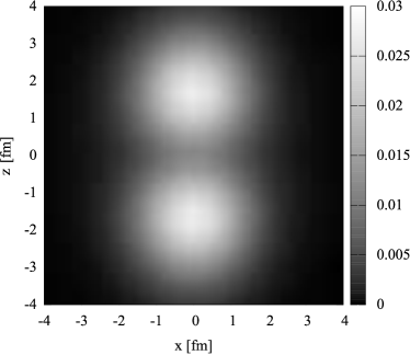
Figure 2: Density distribution of the intrinsic ground state of ⁹Be. The gray scale of each point in the figure stands for the nucleon density on $x-z$ plane of the $y=0$ cross section. The unit of the density is fm^-3.

To get a clear view of the binding effect of the extra neutron and the structure of the ground state, we also calculate the density distribution $\rho(\mathbf{r}^{\prime}_{n})$ of the extra nucleon. The intrinsic wave function $\Psi$ can be written in the form of,

$$\Psi=\text{C}\hat{A}[\Phi^{\text{THSR}}(2\alpha)\phi_{n}(\mathbf{r})],$$ (18)

where $\hat{A}$ is the antisymmetrizer, and C is the normalization constant. Then we can define the density distribution $\rho(\mathbf{r}^{\prime}_{n})$ of the extra neutron as

$$\rho(\mathbf{r}^{\prime}_{n})=\sqrt{9}\langle\Phi^{\text{THSR}}(2\alpha)\phi_{n}(\mathbf{r})|\delta(\mathbf{r}-\mathbf{X}_{G}-\mathbf{r}^{\prime}_{n})|\Psi\rangle,$$ (19)

where $\sqrt{9}$ comes from the normalization constant Horiuchi1977 . As shown in Fig. 3, a distribution result which consists of two parts is displayed on the $y=0$ cross section and a ring style distribution can be seen on the $z=0$ cross section. This distribution, in which the extra neutron cannot stay along the $z$-axis, originates from the restriction of rotational symmetry by the phase factor $e^{i\phi_{\mathbf{R}_{n}}}$. However, this restriction is reasonable because similar distribution has been given by previous GCM calculations Okabe1977 ; Okabe1979 . The distribution of the extra nucleon spreads more than 6 fm in $z$ direction, which is about double the size of each $\alpha$ cluster. It also has overlaps with distributions of both $\alpha$ clusters, which is known as the $\pi$ orbit in nuclear Molecular Orbit model. This is interesting because, at variance with previous works in Ref. Oertzen1996 and Ref. Itagaki2000 , no molecular orbit is presumed in our wave function. In the THSR wave function, the extra nucleon is only assumed to make a nonlocalized motion inside the nucleus. The $\pi$-orbit emerges naturally from the antisymmetrization which cancels out nonphysical distributions. This reproduction of nuclear molecular orbit structure provides another support for our extension of the nonlocalized clustering concept to ⁹Be.

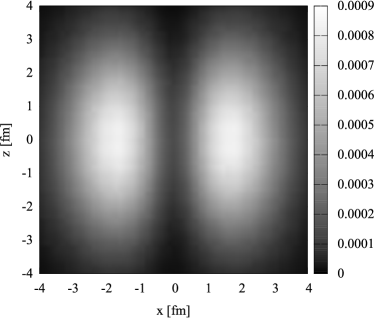
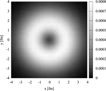
Figure 3: Density distribution $\rho(\mathbf{r}^{\prime}_{n})$ of the extra neutron of the intrinsic ground state of ⁹Be. The gray scale of each point in left part (a) of the figure stands for the nucleon density on $x-z$ plane of the $y=0$ cross section. The gray scale of each point in right part (b) of the figure stands for the nucleon density on $x-y$ plane of the $z=0$ cross section. The unit of the density is fm^-3.

Table 2: Comparison of results form the THSR wave function and the nuclear Molecular Orbit model. $E$ is the binding energy in MeV. “THSR” denotes the result calculated with THSR wave function. “MO” denotes the result of Molecular Orbit model and “MO+GCM” is the result of Molecular Orbit model plus GCM technique. Parameter $b=1.46$ fm as used in Ref. Itagaki2000 . Other parameters are variationally optimized.

Model	$b$ (fm)	$E(3/2^{-})$ (MeV)
THSR	1.46	54.7
MO Itagaki2000	1.46	54.8
MO + GCM Itagaki2000	1.46	56.1

To compare the THSR wave function with the nuclear molecular orbit model, we use $b=1.46$ fm which is the same value as in Ref. Itagaki2000 . The calculated binding energy of the ground state $3/2^{-}$ with different models but same interaction and parameter $b$ are listed in Table 2. With the THSR wave function, we get a value of -54.7 MeV for the binding energy of the ground state, which is almost the same as the result of the Molecular Orbit (MO) Model without GCM technique in Ref. Itagaki2000 . This agreement shows that the motion of the valence neutron in ⁹Be is well treated with the THSR wave function. Comparison with the result of MO+GCM method in Ref. Itagaki2000 shows that our result is about 1.3 MeV higher. This is acceptable because the results of MO+GCM method should be compared with results of THSR+GCM model rather than with those from a single THSR wave function.

We consider that both $3/2^{-}$ ground state and other states such as $1/2^{+}$ state will be well described by single THSR wave functions. This paper has shown that really a single THSR wave function well describes the $3/2^{-}$ ground state. In our near-future paper we will study the $1/2^{+}$ state.

IV Conclusion

We extended the nonlocalized clustering concept inherent to the THSR wave function to the $N\not=Z$ nucleus ⁹Be, in which the $\alpha$-clusters and extra neutron make nonlocalized motion inside the nucleus. We introduce a modified version of the THSR wave function that includes a creation operator of the extra neutron. With the introduced phase factor $e^{im\phi_{\mathbf{R}}}$, our wave function has intrinsic negative parity for $m=\pm 1$. Binding energies are calculated for the $3/2^{-}$ rotational band head of ⁹Be by the variational method. The calculated binding energy from the THSR wave function fits well with the Brink+GCM results. The excitation energies of two excited states are also reasonable compared with the experimental results. The squared overlap between the THSR wave function and the Brink+GCM wave function are found to be close to 96%. This means that the THSR wave function provides a good description of the $3/2^{-}$ rotational band head of ⁹Be. With the same parameter $b=1.46$ fm, our result for the binding energy of the ground state is consistent with the Molecular Orbit (MO) model but higher than in the MO+GCM model. The calculated RMS radius of the ground state also agrees well with the experimental value. By calculating density distributions of the ground state of ⁹Be, the $\pi$-orbit structure is naturally reproduced by the THSR wave function without ad hoc assumption. The calculation of ⁹Be provides support for the extension of the nonlocalized clustering concept to $N\not=Z$ nuclei. It also shows to possess the flexibility to describe other structures such as nuclear molecular orbital structure with the THSR wave function. Though with our technique we essentially have not found anything for the ⁹Be structure which was not known before, we think that it is interesting to see that the THSR wave function also works with adding valence neutrons to the $\alpha$ particles. This is because it is shown that the geometrical cluster structures arise only from kinematical reasons which is a new aspect of cluster physics. Otherwise clusters and extra neutrons are free in their motion.

*

Appendix A The derivation of the single form of the THSR wave function with $m=1$

The THSR wave function of ⁹Be can be write in $r$ space as

$$\begin{split}&\langle\mathbf{r}_{1},\sigma_{1},\tau_{1},\dots,\mathbf{r}_{n},\sigma_{n},\tau_{n}\left|\Phi\right\rangle\\ =&\int d\mathbf{R}_{1}\int d\mathbf{R}_{2}\int d\mathbf{R}_{n}\prod_{i=1,2,n}\prod_{k=x,y,z}\exp\left\{-\frac{R_{i,k}^{2}}{\beta_{i,k}^{2}}\right\}\exp\{i\phi_{\mathbf{R}_{n}}\}\Phi^{B}(\mathbf{R}_{1},\mathbf{R}_{2},\mathbf{R}_{n})\end{split}$$ (20)

where $\Phi^{B}$ is the Brink wave function. To obtain the single function form of the THSR wave function, we need to perform the integration of the generate coordinates $\mathbf{R}_{1}$, $\mathbf{R}_{2}$ and $\mathbf{R}_{n}$ in Eq. (20) analytically. Because the Brink wave function is the antisymmetrization of single nucleon wave functions, this integration over different generate coordinates can be performed separately.

The integration over two $\alpha$-cluster generate coordinates $\mathbf{R}_{1}$ and $\mathbf{R}_{2}$ is already given as $F_{\alpha}(\mathbf{R}_{1},\mathbf{R}_{2})\phi(\alpha_{1})\phi(\alpha_{2})$ in Ref. Tohsaki2001 , where $\Psi(\alpha)$ is the internal $\alpha$-cluster wave function, and the motion of the center-of-mass of $\alpha$-clusters is

$$\begin{split}F_{\alpha}(\mathbf{X}_{1},\mathbf{X}_{2})=\exp\left\{-\frac{X_{1,x}^{2}+X_{1,y}^{2}+X_{2,x}^{2}+X_{2,y}^{2}}{C_{\alpha,xy}^{2}}-\frac{X_{1,z}^{2}+X_{2,z}^{2}}{C_{\alpha,z}^{2}}\right\},\\ \end{split}$$ (21)

where $C_{\alpha,xy}^{2}=b^{2}/2+\beta_{\alpha,xy}^{2}$ and $C_{\alpha,z}^{2}=b^{2}/2+\beta_{\alpha,z}^{2}$.

The integration over generate coordinate $\mathbf{R}_{n}$ for the extra neutron can be separated into two integration of its different components. The first one is the integration over its $z$-component $R_{n,z}$ as,

$$\begin{split}f_{n,z}(r_{n,z})=&\int dR_{n,z}\exp\left\{-\frac{R_{n,z}^{2}}{\beta_{n,z}^{2}}\right\}\exp\left\{-\frac{1}{2b^{2}}(r_{n,z}-R_{n,z})^{2}\right\}\\ \propto&\exp\left\{-\frac{r_{n,z}^{2}}{C_{n,z}^{2}}\right\}\end{split}$$ (22)

where $C_{n,z}^{2}=2b^{2}+\beta_{n,z}^{2}$. Another one is the integration over its $x$-component $R_{n,x}$ and $y$-component $R_{n,y}$ as

$$\begin{split}f_{n,xy}(r_{n,x},r_{n,y})=\int dR_{n,x}dR_{n,y}&\exp\left\{-\frac{R_{n,x}^{2}+R_{n,y}^{2}}{\beta_{n,xy}^{2}}\right\}e^{i\phi_{\mathbf{R}_{n}}}\\ &\times\exp\left\{-\frac{1}{2b^{2}}[(r_{n,x}-R_{n,x})^{2}+(r_{n,y}-R_{n,y})^{2})]\right\}.\end{split}$$ (23)

This integration of $R_{n,x}$ and $R_{n,y}$ can be rewritten in polar coordinate system as

$$\begin{split}f_{n,xy}(r_{n,x},r_{n,y})=\int_{0}^{2\pi}d\phi_{R}\int_{0}^{\infty}\rho_{R}d\rho_{R}&\exp\left\{-\frac{\rho^{2}_{R}}{\beta_{n,xy}^{2}}\right\}e^{i\phi_{R}}\\ &\times\exp\left\{-\frac{1}{2b^{2}}[\rho^{2}_{R}+\rho_{r}^{2}+2\rho_{R}\rho_{r}\cos(\phi_{R}-\phi_{r})]\right\},\end{split}$$ (24)

where $\rho_{R}=(R_{n,x}^{2}+R_{n,y}^{2})^{1/2}$, $\rho_{r}=(r_{n,x}^{2}+r_{n,y}^{2})^{1/2}$, and $\phi_{R}$ and $\phi_{r}$ are angles of vector $(R_{n,x},R_{n,y})$ and $(r_{n,x},r_{n,y})$ in polar coordinate system respectively. Obviously, we have $\phi_{R}=\phi_{\mathbf{R}_{n}}$, where $\phi_{\mathbf{R}_{n}}$ is the azimuthal angle of $\mathbf{R}_{n}$ in spherical coordinate system.

As a first step, the integration over radial coordinate $\rho_{R}$ is performed as

$$\begin{split}&\int\rho_{R}d\rho_{R}\exp\left\{-\frac{\rho^{2}_{R}}{\beta_{n,xy}^{2}}-\frac{1}{2b^{2}}[\rho^{2}_{R}+\rho_{r}^{2}+2\rho_{R}\rho_{r}\cos(\phi_{R}-\phi_{r})]\right\}\\ \propto&\exp\left\{-\frac{1}{2b^{2}}\rho_{r}^{2}\right\}\\ &\times\left\{a+\sqrt{\pi}\rho_{r}\cos(\phi_{R}-\phi_{r})[\text{Erf}(\rho_{r}\cos(\phi_{R}-\phi_{r})/a)-1]\exp(\rho_{r}^{2}\cos^{2}(\phi_{R}-\phi_{r})/a^{2})\right\},\end{split}$$ (25)

where $a=\sqrt{2b^{2}+4b^{4}/\beta_{xy}^{2}}$.

The next step is to integrate over the angle $\phi_{R}$. Since $\int_{0}^{2\pi}\exp(i\phi_{R})d\phi_{R}=0$, we can safely omit the first constant $a$ in Eq. (25) as

$$\begin{split}f_{n,xy}(r_{n,x},r_{n,y})\propto\int_{0}^{2\pi}d\phi_{R}&\exp\left\{-\frac{1}{2b^{2}}\rho_{r}^{2}+i\phi_{R}\right\}\rho_{r}\cos(\phi_{R}-\phi_{r})\\ &\times[\text{Erf}(\rho_{r}\cos(\phi_{R}-\phi_{r})/a)-1]\exp(\rho_{r}^{2}\cos^{2}(\phi_{R}-\phi_{r})/a^{2}).\end{split}$$ (26)

Then the substitution $\phi_{R}\rightarrow\phi_{R}-\phi_{r}+\phi_{r}$ is applied to the equation above as

$$\begin{split}f_{n,xy}(r_{n,x},r_{n,y})\propto\int_{0}^{2\pi}d\phi_{R}&\exp\left\{-\frac{1}{2b^{2}}\rho_{r}^{2}+i\phi_{r}\right\}e^{i(\phi_{R}-\phi_{r})}(\rho_{r}\cos(\phi_{R}-\phi_{r}))\\ &\times[\text{Erf}(\rho_{r}\cos(\phi_{R}-\phi_{r})/a)-1]\exp(\rho_{r}^{2}\cos^{2}(\phi_{R}-\phi_{r})/a^{2}).\end{split}$$ (27)

Since $f_{n,xy}(r_{n,x},r_{n,y})$ is a periodic function of $\phi_{R}$ with a $2\pi$ period, the integration over $\phi_{R}$ can be written as

$$\begin{split}f_{n,xy}(r_{n,x},r_{n,y})\propto\int_{0}^{2\pi}&\exp\left\{-\frac{1}{2b^{2}}\rho_{r}^{2}+i\phi_{r}\right\}e^{i\theta}(\rho_{r}\cos\theta)\\ &\times[\text{Erf}(\rho_{r}\cos\theta/a)-1]\exp(\rho_{r}^{2}\cos^{2}\theta/a^{2})d\theta,\end{split}$$ (28)

where $\theta=\phi_{R}-\phi_{r}$.

Considering the Euler equation $e^{i\theta}=\cos\theta+i\sin\theta$, the integration above is divided into two terms, one with the real part $\cos\theta$ and one with the imaginary part $i\sin\theta$. The term with $i\sin\theta$ can be easily obtained as

$$\begin{split}&\int_{0}^{2\pi}i\sin\theta(\rho_{r}\cos\theta)[\text{Erf}(\rho_{r}\cos\theta/a)-1]\exp(\rho_{r}^{2}\cos^{2}\theta/a^{2})d\theta\\ =&-\int_{0}^{2\pi}i\rho_{r}\cos\theta[\text{Erf}(\rho_{r}\cos\theta/a)-1]\exp(\rho_{r}^{2}\cos^{2}\theta/a^{2})d\cos\theta\\ =&-\left(\int_{1}^{-1}+\int_{-1}^{1}\right)i\rho_{r}t[\text{Erf}(\rho_{r}t/a)-1]\exp(\rho_{r}^{2}t^{2}/a^{2})dt\\ =&0.\end{split}$$ (29)

Now the remaining term in $f_{n,xy}(r_{n,x},r_{n,y})$ is

$$\begin{split}f_{n,xy}(r_{n,x},r_{n,y})\propto\int_{0}^{2\pi}&\exp\left\{-\frac{1}{2b^{2}}\rho_{r}^{2}+i\phi_{r}\right\}\frac{1}{\rho_{r}}(\rho_{r}\cos\theta/a)^{2}\\ &\times[\text{Erf}(\rho_{r}\cos\theta/a)-1]\exp(\rho_{r}^{2}\cos^{2}\theta/a^{2})d\theta.\\ \end{split}$$ (30)

The integration over $\theta$ can be obtained analytically with Mathematica as

$$\begin{split}&\int_{0}^{2\pi}(\rho_{r}\cos\theta/a)^{2}[\text{Erf}(\rho_{r}\cos\theta/a)-1]\exp(\rho_{r}^{2}\cos^{2}\theta/a^{2})d\theta\\ =&-\frac{\pi\rho_{r}^{2}}{a^{2}}\exp\left\{\frac{\rho_{r}^{2}}{(2a^{2})}\right\}\left[I_{0}\left(\frac{\rho_{r}^{2}}{2a^{2}}\right)+I_{1}\left(\frac{\rho_{r}^{2}}{2a^{2}}\right)\right],\end{split}$$ (31)

where $I_{0}$ and $I_{1}$ are the modified Bessel functions of the first kind. We will show the proof of Eq. (31) later. Substitute this equation into $f_{n,xy}(r_{n,x},r_{n,y})$ and we have

$$\begin{split}&f_{n,xy}(r_{n,x},r_{n,y})\propto\exp\left\{(\frac{1}{2a^{2}}-\frac{1}{2b^{2}})\rho_{r}^{2}+i\phi_{r}\right\}\rho_{r}\left[I_{0}\left(\frac{\rho_{r}^{2}}{2a^{2}}\right)+I_{1}\left(\frac{\rho_{r}^{2}}{2a^{2}}\right)\right].\end{split}$$ (32)

which can be written as

$$\begin{split}f_{n,xy}(r_{n,x},r_{n,y})\propto&\exp\left\{-\frac{r_{n,x}^{2}+r_{n,y}^{2}}{C_{n,xy}^{2}}\right\}\\ &\times[I_{0}(\frac{r_{n,x}^{2}+r_{n,y}^{2}}{A^{2}})+I_{1}(\frac{r_{n,x}^{2}+r_{n,y}^{2}}{A^{2}})]\\ &\times(r_{n,x}^{2}+r_{n,y}^{2})^{1/2}e^{i\phi_{r_{n}}},\end{split}$$ (33)

where

$$\begin{split}C_{n,xy}^{2}=-\left(\frac{1}{2a^{2}}-\frac{1}{2b^{2}}\right)^{-1}=\frac{8b^{4}+4b^{2}\beta_{n,xy}^{2}}{4b^{2}+\beta_{n,xy}^{2}},\end{split}$$ (34)

and

$$\begin{split}A^{2}=2a^{2}=4b^{2}+\frac{8b^{4}}{\beta_{n,xy}^{2}}.\end{split}$$ (35)

Thus we have obtained analytically all the integration results of the generate coordinates , and the THSR wave function can now be written in the single function form as,

$$\langle\mathbf{r}_{1},\sigma_{1},\tau_{1},\dots,\mathbf{r}_{n},\sigma_{n},\tau_{n}\left|\Phi\right\rangle\propto\mathcal{A}\left[F(\mathbf{X}_{1},\mathbf{X}_{2},\mathbf{r}_{n})\phi(\alpha_{1})\phi(\alpha_{2})\right]$$ (36)

where

$$\begin{split}F(\mathbf{X}_{1},\mathbf{X}_{2},\mathbf{r}_{n})=&F_{\alpha}(\mathbf{R}_{1},\mathbf{R}_{2})f_{n,xy}(r_{n,x},r_{n,y})f_{n,z}(r_{n,z})\\ =&\exp\left\{-\frac{X_{1,x}^{2}+X_{1,y}^{2}+X_{2,x}^{2}+X_{2,y}^{2}}{C_{\alpha,xy}^{2}}-\frac{X_{1,z}^{2}+X_{2,z}^{2}}{C_{\alpha,z}^{2}}\right\}\\ &\times\exp\left\{-\frac{r_{n,x}^{2}+r_{n,y}^{2}}{C_{n,xy}^{2}}-\frac{r_{n,z}^{2}}{C_{n,z}^{2}}\right\}\\ &\times[I_{0}(\frac{r_{n,x}^{2}+r_{n,y}^{2}}{A^{2}})+I_{1}(\frac{r_{n,x}^{2}+r_{n,y}^{2}}{A^{2}})]\\ &\times(r_{n,x}^{2}+r_{n,y}^{2})^{1/2}e^{\pm i\phi_{r_{n}}}\end{split}$$ (37)

where  $C_{\alpha,xy}^{2}=b^{2}/2+\beta_{\alpha,xy}^{2}$,  $C_{\alpha,z}^{2}=b^{2}/2+\beta_{\alpha,z}^{2}$,  $C_{n,xy}^{2}=(8b^{4}+4b^{2}\beta_{n,xy}^{2})/(4b^{2}+\beta_{n,xy}^{2})$,  $C_{n,z}^{2}=2b^{2}+\beta_{n,z}^{2}$,  and  $A^{2}=4b^{2}+8b^{4}/\beta_{n,xy}^{2}$.

Proof of Eq. (A.12) in the Appendix

We will apply the substitution $t=\rho_{r}/a$ in Eq. (A.12) and prove the following integral,

$$\begin{split}\int_{0}^{2\pi}&t^{2}\cos^{2}\theta[\text{Erf}(t\cos\theta)-1]\exp(t^{2}\cos^{2}\theta)d\theta\\ &=-\pi t^{2}\exp\left(\frac{t^{2}}{2}\right)\left[I_{0}\left(\frac{t^{2}}{2}\right)+I_{1}\left(\frac{t^{2}}{2}\right)\right],\end{split}$$ (38)

First we evaluate the integral of the first term in $[\cdots]$ in the left side in Eq. (38):

$$\begin{split}\int_{0}^{2\pi}&t^{2}\cos^{2}\theta\text{Erf}(t\cos\theta)\exp(t^{2}\cos^{2}\theta)d\theta\\ &=\int_{0}^{\pi/2}\cdots d\theta+\int_{\pi/2}^{\pi}\cdots d\theta+\int_{\pi}^{3\pi/2}\cdots d\theta+\int_{3\pi/2}^{2\pi}\cdots d\theta.\end{split}$$ (39)

The third term in Eq. (39) can be written as

$$\begin{split}\int_{\pi}^{3\pi/2}&t^{2}\cos^{2}\theta\text{Erf}(t\cos\theta)\exp(t^{2}\cos^{2}\theta)d\theta\\ &=\int_{0}^{\pi/2}t^{2}\cos^{2}\theta\text{Erf}(-t\cos\theta)\exp(t^{2}\cos^{2}\theta)d\theta\\ &=-\int_{0}^{\pi/2}t^{2}\cos^{2}\theta\text{Erf}(t\cos\theta)\exp(t^{2}\cos^{2}\theta)d\theta.\\ \end{split}$$ (40)

Thus the sum of the first and third terms in Eq. (39) is zero. In the same manner the sum of the second and fourth terms in Eq. (39) is zero. Then the result of Eq. (39) can be written as

$$\int_{0}^{2\pi}t^{2}\cos^{2}\theta\text{Erf}(t\cos\theta)\exp(t^{2}\cos^{2}\theta)d\theta=0.$$ (41)

Thus we have to prove the following equation:

$$\int_{0}^{2\pi}\cos^{2}\theta\exp(t^{2}\cos^{2}\theta)d\theta=\pi\exp\left(\frac{t^{2}}{2}\right)\left[I_{0}\left(\frac{t^{2}}{2}\right)+I_{1}\left(\frac{t^{2}}{2}\right)\right].$$ (42)

With use of a simple formula, $\cos^{2}\theta=(\cos 2\theta+1)/2$, Equation (42) can be written as

$$\int_{0}^{2\pi}(1+\cos 2\theta)\exp\left(\frac{t^{2}}{2}\cos 2\theta\right)d\theta=2\pi\left[I_{0}\left(\frac{t^{2}}{2}\right)+I_{1}\left(\frac{t^{2}}{2}\right)\right].$$ (43)

Next we will prove Eq. (43). For simplicity, we apply the substitution of $z=t^{2}/2$.

$$\begin{split}\int_{0}^{2\pi}\exp\left(z\cos 2\theta\right)d\theta&=\int_{0}^{2\pi}\exp\left(z\cos\theta\right)d\theta\\ &=\sum_{n=0}^{\infty}\frac{z^{n}}{n!}\int_{0}^{2\pi}(\cos\theta)^{n}d\theta\end{split}$$ (44)

With use of the following formula,

$$\int_{0}^{2\pi}(\cos\theta)^{n}d\theta\left\{\begin{array}[]{cl}2\sqrt{\pi}\,\Gamma(k+\frac{1}{2})/\Gamma(k+1)&\text{for }n=2k\\ 0&\text{for }n=\text{odd}\\ \end{array}\right.,$$ (47)

$$\Gamma\left(k+\frac{1}{2}\right)=\frac{\sqrt{\pi}(2k)!}{2^{2k}k!}$$ (48)

$$I_{\nu}(z)=\left(\frac{z}{2}\right)^{\nu}\sum_{k=0}^{\infty}\frac{1}{k!\Gamma(\nu+k+1)}\left(\frac{z}{2}\right)^{2k},$$ (49)

we can write down as follows,

$$\begin{split}\int_{0}^{2\pi}&\exp(z\cos\theta)d\theta\\ &=\sum_{k=0}^{\infty}\frac{z^{2k}}{(2k)!}\int_{0}^{2\pi}(\cos\theta)^{2k}d\theta\\ &=2\pi\sum_{k=0}^{\infty}\frac{1}{k!\Gamma(k+1)}\left(\frac{z}{2}\right)^{2k}\\ &=2\pi I_{0}(z).\end{split}$$ (50)

On the other hand,

$$\begin{split}\int_{0}^{2\pi}&\cos 2\theta\exp(z\cos 2\theta)d\theta\\ &=\int_{0}^{2\pi}\cos\theta\exp(z\cos\theta)d\theta\\ &=\sum_{n=0}^{\infty}\frac{z^{n}}{n!}\int_{0}^{2\pi}(\cos\theta)^{n+1}d\theta\\ &=\sum_{k=0}^{\infty}\frac{z^{2k+1}}{(2k+1)!}\int_{0}^{2\pi}(\cos\theta)^{2k+2}d\theta\\ &=2\pi\times\left(\frac{z}{2}\right)\sum_{k=0}^{\infty}\frac{1}{k!\Gamma(k+2)}\left(\frac{z}{2}\right)^{2k}\\ &=2\pi I_{1}(z).\end{split}$$ (51)

Then Eqs. (43) and (38) were proved.

References

• (1) A. Tohsaki, H. Horiuchi, P. Schuck, and G. Röpke, Phys. Rev. Lett. 87, 192501 (2001).
• (2) T. Yamada and P. Schuck, Eur. Phys. J. A 26, 185 (2005).
• (3) Y. Funaki, H. Horiuchi, A. Tohsaki, P. Schuck, and G. Röpke, Prog. Theor. Phys. 108, 297 (2002).
• (4) B. Zhou, Y. Funaki, H. Horiuchi, Z. Ren, G. Röpke, P. Schuck, A. Tohsaki, C. Xu, and T. Yamada, Phys. Rev. Lett. 110, 262501 (2013).
• (5) C. Xu and Z. Ren, Phys. Rev. C 73, 041301 (2006).
• (6) Y. Ren and Z. Ren, Phys. Rev. C 85, 044608 (2012).
• (7) B. Zhou, Z. Ren, C. Xu, Y. Funaki, T. Yamada, A. Tohsaki, H. Horiuchi, P. Schuck, and G. Röpke, Phys. Rev. C 86, 014301 (2012).
• (8) B. Zhou, Y. Funaki, H. Horiuchi, Z. Ren, G. Röpke, P. Schuck, A. Tohsaki, C. Xu, and T. Yamada, Phys. Rev. C 89, 034319 (2014).
• (9) A. Tohsaki, Int. J. Mod. Phys. E 17, 2106 (2008).
• (10) Y. Kanada-En’yo, H. Horiuchi, and A. Ono, Phys. Rev. C 52, 628 (1995).
• (11) S. Okabe, Y. Abe, and H. Tanaka, Prog. Theor. Phys. 57, 866 (1977).
• (12) N. Itagaki and S. Okabe, Phys. Rev. C 61, 044306 (2000).
• (13) W. von Oertzen, Z. Phys. A 354, 37 (1996).
• (14) P. Ring and P. Schuck, The Nuclear Many-Body Problem (Springer-Verlag, New York, 1980), p. 474.
• (15) A.B. Volkov, Nucl. Phys. 74, 33 (1965).
• (16) N. Yamaguchi, T. Kasahara, S. Nagata, and Y. Akaishi, Prog. Theor. Phys. 62, 1018 (1979).
• (17) S. Okabe and Y. Abe, Prog. Theor. Phys. 61, 1049 (1979).
• (18) D. R. Tilley, J. H. Kelley, J. L. Godwin, D. J. Millener, J. E. Purcell, C. G. Sheu, and H. R. Weller, Nucl. Phys. A 745, 155 (2004).
• (19) G. Audi, F. G. Kondev, M. Wang, B. Pfeiffer, X. Sun, J. Blachot, and M. MacCormick, Chin. Phys. C 36, 1157 (2012).
• (20) I. Tanihata, H. Hamagaki, O. Hashimoto, Y. Shida, N. Yoshikawa, K. Sugimoto, O. Yamakawa, T. Kobayashi, and N. Takahashi, Phys. Rev. Lett. 55, 2676 (1985).
• (21) H. Horiuchi, Prog. Theor. Phys. Supple. 62, 90 (1977).