Quantized electromagnetic response of three-dimensional chiral topological insulators

Abstract

Protected by the chiral symmetry, three dimensional chiral topological insulators are characterized by an integer-valued topological invariant. How this invariant could emerge in physical observables is an important question. Here we show that the magneto-electric polarization can identify the integer-valued invariant if we gap the system without coating a quantum Hall layer on the surface. The quantized response is demonstrated to be robust against weak perturbations. We also study the topological properties by adiabatically coupling two nontrivial phases, and find that gapless states appear and are localized at the boundary region. Finally, an experimental scheme is proposed to realize the Hamiltonian and measure the quantized response with ultracold atoms in optical lattices.

I Introduction

The periodic table of topological insulators (TIs) and superconductors classifies topological phases of free fermions according to the system symmetry and spatial dimensions Schnyder et al. (2008); Kitaev (2009). Notable examples include integer quantum Hall insulators breaking all those classification symmetries and the time-reversal-invariant TIs protected by the time-reversal symmetry Hasan and Kane (2010); Moore (2010); Qi and Zhang (2011); Kane and Mele (2005); Bernevig et al. (2006); Fu et al. (2007). Mathematically, these exotic states can be characterized by various topological invariants. An interesting question is how to relate these invariants to physical observables. For integer quantum Hall insulators, the Chern number ($\mathbb{Z}$ invariant) corresponds to the quantized Hall conductance Thouless et al. (1982), while for the time-reversal-invariant TIs, the $\mathbb{Z}_{2}$ invariant is associated with a quantized magneto-electric effect in three dimensions (3D) Qi et al. (2008); Essin et al. (2009).

The 3D chiral TIs protected by the chiral symmetry Hosur et al. (2010); Ryu et al. (2010) are of particular interest as they are 3D TIs characterized by a $\mathbb{Z}$ (instead of $\mathbb{Z}_{2}$) invariant and may be realized in ultracold atomic gases with engineered spin-orbital coupling Lewenstein et al. (2007); Dalibard et al. (2011); Goldman et al. (2014). An experimental scheme was recently proposed to implement a three-band chiral TI in an optical lattice Wang et al. (2014). For such 3D chiral TIs, it is known that the topological magneto-electric effect should also arise, but in theory it captures only the $\mathbb{Z}_{2}$ part of the $\mathbb{Z}$ invariant due to the gauge dependence of the polarization in translationally invariant systems Hosur et al. (2010). It is thus an important question to find out how the $\mathbb{Z}$ character could manifest itself in experiments. It was proposed in Ref. Shiozaki and Fujimoto (2013) that the $\mathbb{Z}$ effect may become visible in certain carefully engineered heterostructures, but the implementation of such a heterostructure is experimentally challenging.

In this paper, we study the nontrivial $\mathbb{Z}$ character of the chiral TI by exploring the adiabatic transition between two nontrivial phases and by numerically simulating the magneto-electric effect in a single phase. We show that not only the $\mathbb{Z}_{2}$ response but the $\mathbb{Z}$ character can be observed by gapping the system without adding a quantum Hall layer on the surface, i.e., the ambiguity resulting from different terminations appears to be avoidable in practice. Also, the quantized polarization is demonstrated to be robust against small perturbations even in the absence of a perfect chiral symmetry. This observation is important for experimental realization, because in a real system the chiral symmetry is typically an approximate instead of exact symmetry. Lastly, we propose an experimental scheme to realize the Hamiltonian and probe the integrally quantized response with cold atomic systems.

II Model and Topological Characterization

We first introduce a minimal lattice tight-binding model for chiral topological insulators with the Hamiltonian in the momentum space given by $H_{1}=\sum_{\mathbf{k}}\Psi_{\mathbf{k}}^{\dagger}\mathcal{H}_{1}(\mathbf{k})\Psi_{\mathbf{k}}$, where $\Psi_{\mathbf{k}}=(a_{\mathbf{k\uparrow}},a_{\mathbf{k}\downarrow},b_{\mathbf{k}\uparrow},b_{\mathbf{k}\downarrow})^{T}$ denotes fermionic annihilation operators with spins $\uparrow,\downarrow$ on sublattices or orbitals $a,b$. In cold atom systems, the pseudospins and orbitals can be represented by different atomic internal states. The $4\times 4$ Hamiltonian is

$$\mathcal{H}_{1}(\mathbf{k})\!=\!\left(\!\begin{array}[]{cccc}0&0&-iq_{0}+q_{3}&q_{1}-iq_{2}\\ 0&0&q_{1}+iq_{2}&-iq_{0}-q_{3}\\ iq_{0}+q_{3}&q_{1}-iq_{2}&0&0\\ q_{1}+iq_{2}&iq_{0}-q_{3}&0&0\end{array}\!\!\right)$$ (1)

where $q_{0}=h+\cos k_{x}+\cos k_{y}+\cos k_{z},q_{1}=\sin k_{x}+\delta,q_{2}=\sin k_{y},q_{3}=\sin k_{z}$, with $h,\delta$ being control parameters. The lattice constant and tunneling energy are set to unity. In real space, this Hamiltonian represents on-site and nearest neighbor hoppings and spin-flip hoppings between two orbitals in a simple cubic lattice. These hoppings can be realized by two-photon Raman transitions in cold atoms Jaksch and Zoller (2003); Aidelsburger et al. (2013); Miyake et al. (2013); Wang et al. (2014). The energy spectrum for this Hamiltonian is $E_{\pm}(\mathbf{k})=\pm[(\sin k_{x}+\delta)^{2}+\sin^{2}k_{y}+\sin^{2}k_{z}+(\cos k_{x}+\cos k_{y}+\cos k_{z}+h)^{2}]^{1/2}$, with two-fold degeneracy at each $\mathbf{k}$. For $\delta=0$, the system acquires time-reversal symmetry $T$, particle-hole symmetry $C$, and chiral symmetry $S=TC$, which can be explicitly seen as Ryu et al. (2010):

$$T: \quad(\sigma_{x}\otimes\sigma_{y})[\mathcal{H}_{1}(\mathbf{k})]^{\ast}(\sigma_{x}\otimes\sigma_{y}) =\mathcal{H}_{1}(-\mathbf{k})$$ (2)

$$C: \quad(\sigma_{y}\otimes\sigma_{y})[\mathcal{H}_{1}(\mathbf{k})]^{\ast}(\sigma_{y}\otimes\sigma_{y}) =-\mathcal{H}_{1}(-\mathbf{k})$$ (3)

$$S: \quad(\sigma_{z}\otimes I_{2})[\mathcal{H}_{1}(\mathbf{k})](\sigma_{z}\otimes I_{2}) =-\mathcal{H}_{1}(\mathbf{k})$$ (4)

with $\sigma_{i}$ as Pauli matrices, and $I_{2}$ as the $2\times 2$ identity matrix. When $\delta\neq 0$, time-reversal and particle-hole symmetries are explicitly broken, but the chiral symmetry survives.

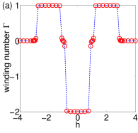
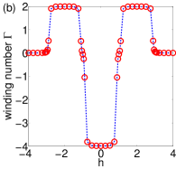
Figure 1: (Color online) The winding number $\Gamma$ as a function of the parameter $h$. The Hamiltonians are $\mathcal{H}_{1}(k)$ in (a) and $\mathcal{H}_{2}(k)$ in (b) respectively. $\delta=0.5$ for both panels.

The topological property of the Hamiltonian $\mathcal{H}_{1}(\mathbf{k})$ can be characterized by the winding number $\Gamma$ Schnyder et al. (2008); Ryu et al. (2010). To define the winding number, let us introduce the $Q$ matrix, $Q(\mathbf{k})=1-2P(\mathbf{k})$, where $P(\mathbf{k})=\sum_{f}|u_{f}(\mathbf{k})\rangle\langle u_{f}(\mathbf{k})|$ is the projector onto the filled Bloch bands with wave-vectors $|u_{f}(\mathbf{k})\rangle$. The $Q$ matrix can be brought into the block off-diagonal form $Q(\mathbf{k)}=\left(\begin{array}[]{cc}0&b(\mathbf{k})\\ b^{\dagger}(\mathbf{k})&0\end{array}\right)$ with the chiral symmetry. With the matrix $b(\mathbf{k})$, one can write Schnyder et al. (2008); Ryu et al. (2010)

$$\Gamma\!=\!\frac{1}{24\pi^{2}}\int_{\text{BZ}}d\mathbf{k}\;\epsilon^{\mu\rho\lambda}\text{Tr}[(b^{-1}\partial_{\mu}b)(b^{-1}\partial_{\rho}b)(b^{-1}\partial_{\lambda}b)],$$ (5)

where $\epsilon^{\mu\rho\lambda}$ is the antisymmetric Levi-Civita symbol and $\partial_{\mu}b\equiv\partial_{k_{\mu}}b(\mathbf{k})$. The Hamiltonian $\mathcal{H}_{1}(\mathbf{k})$ supports topological phases with $\Gamma=1,-2$. To obtain chiral TIs with arbitrary integer topological invariants, one can use the quaternion construction proposed in Ref. Deng et al. (2014a). By considering $q=q_{0}+q_{1}\bm{i}+q_{2}\bm{j}+q_{3}\bm{k}$ as a quaternion and raising to a power, all $\mathbb{Z}$ topological phases can be realized by the family of tight-binding Hamiltonians. By taking the quaternion square, for example, one obtains $q^{2}=q_{0}^{2}-q_{1}^{2}-q_{2}^{2}-q_{3}^{2}+2q_{0}q_{1}\bm{i}+2q_{0}q_{2}\bm{j}+2q_{0}q_{3}\bm{k}$, and we can therefore acquire another tight-binding Hamiltonian $H_{2}=\sum_{\mathbf{k}}\Psi_{\mathbf{k}}^{\dagger}\mathcal{H}_{2}(\mathbf{k})\Psi_{\mathbf{k}}$ with each component of $q^{2}$ replacing the respective components $q_{0},q_{1},q_{2},q_{3}$ in $\mathcal{H}_{1}(\mathbf{k})$. This second Hamiltonian $\mathcal{H}_{2}(\mathbf{k})$ contains next-nearest-neighbor hopping terms. The winding number $\Gamma$ can be calculated numerically by discretizing the Brillouin zone and replacing the integral by a discrete sum Deng et al. (2014a). The results are shown in Fig. 1 for both $\mathcal{H}_{1}(\mathbf{k})$ and $\mathcal{H}_{2}(\mathbf{k})$.

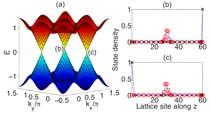
Figure 2: (Color online) Coupling two topologically nontrivial phases by varying the parameter $h$ adiabatically from 0 to 2 along the $z$ direction. $x$ and $y$ directions are periodic. Sixty slabs are taken for the $z$ direction. (a) The energy dispersion for the lowest conduction band and highest valence band. (b) and (c) show the surface states near the respective Dirac points. The $\Gamma$ point is displaced from the center for a better display of the Dirac cones.

III Surface states and Heterostructure of nontrivial topological phases

By imposing an open boundary condition along the $z$ direction, and keeping the $x$ and $y$ directions in momentum space, surface Dirac cones are formed for nontrivial topological phases. We find that the winding number coincides with the total number of Dirac cones counted for all inequivalent surface states (i.e. not counting the twofold degeneracy for each band), which confirms explicitly the bulk-edge correspondence (See Appendix A). A distinctive difference from the time-reversal invariant TI is that any number of Dirac cones on the surface is protected by the chiral symmetry Hosur et al. (2010).

With an integer number of nontrivial phases, it is intriguing to study the topological phase transition between two different phases. A simple way to explore this is to adiabatically vary $h$ from one end to the other end of the sample. The parameter $h$ concerns the onsite tunneling strength between opposite orbitals ($a_{\mathbf{\uparrow}}^{{\dagger}}b_{\mathbf{\uparrow}}$ and $a_{\mathbf{\downarrow}}^{{\dagger}}b_{\mathbf{\downarrow}}$ terms). This hopping can be realized by a two-photon Raman process, and the strength $h$ can be controlled by the laser intensity Wang et al. (2014). Numerically, we vary $h$ in the form of $h=1+\tanh(z-L_{z}/2)$, where $z$ denotes the $z$th layer and $L_{z}$ the total number of slabs along the $z$ direction. This form ensures that $h$ changes adiabatically from $0$ on one end to $2$ on the other end of the sample, so that it effectively couples two nontrivial phases. For the Hamiltonian $\mathcal{H}_{1}$, it couples two topological phases with winding numbers $\Gamma=-2$ and $\Gamma=1$. Similar to the interface between a topological insulator and the trivial vacuum, a surface state should appear at the interface. As shown in Fig. 2, three Dirac cones are formed inside the band gap. In addition to the surface states observed on both ends of the sample, a localized state is formed at the interface between two topologically distinct regions. These interface states are always present regardless of the detailed structure of the interface. Even for sharp boundaries, the interface states remain. The Dirac cone structure may be probed through Bragg spectroscopy in cold atom experiments Stamper-Kurn et al. (1999); Zhu et al. (2007).

The above heterostructure could be used to probe the topological properties of the chiral TI, but it is experimentally difficult to engineer such a heterostructure, especially in cold atom systems. In Ref. Shiozaki and Fujimoto (2013), it was shown that the $\mathbb{Z}$ character of the topological invariant could be seen in some carefully engineered heterostructures. In the following, we show that the $\mathbb{Z}$ topological invariant can be observed via the magneto-electric polarization in a single nontrivial phase with a gapped surface. We further show that the detection will be robust to realistic experimental perturbations and present a feasible experimental scheme to observe the quantized response.

IV Magneto-electric effect

Figure 3: (color online). Charge $Q$ accumulated on the surface in the $z$ direction due to a uniform magnetic field with total flux $\Phi$ at $k_{x}=k_{y}=0$. $N=199,L_{z}=20$ for all three panels. (a) and (b) consider the perturbative effect of an intra-site nearest neighbor hopping. (c) adds a random onsite potential characterized by $\Delta_{\text{rp}}$. The insets show the charge density at $\Phi=3\Phi_{0}$ without perturbations, and a closeup for the slope. The parameters in each panel are: (a) Hamiltonian $\mathcal{H}_{1}(\mathbf{k})$ with $h=2,\delta=0.5,\Delta_{S}=1,\Gamma=1$; (b) Hamiltonian $\mathcal{H}_{2}(\mathbf{k})$ with $h=0,\delta=0,\Delta_{S}=1,\Gamma=-4$; (c) Hamiltonian $\mathcal{H}_{1}(\mathbf{k})$ with $h=2,\delta=0,\Delta_{S}=1,\Gamma=1$. In all panels, the accumulated charge $Q$ is relative to the case when $\Phi=0$ and is summed over all particle species for the upper half of the sample at half fillings.

The magneto-electric effect is a remarkable manifestation of the bulk non-trivial topology. The linear response of a TI to an electromagnetic field can be described by the magneto-electric polarizability tensor as Essin et al. (2009)

$$\alpha_{ij}=\dfrac{\partial P_{i}}{\partial B_{j}}\bigg{|}_{E=0}=\dfrac{\partial M_{j}}{\partial E_{i}}\bigg{|}_{B=0},$$ (6)

where $E$ and $B$ are the electric and magnetic field, $P$ and $M$ are the polarization and magnetization. Unique to topological insulators is a diagonal contribution to the tensor with $\alpha_{ij}=\theta\frac{e^{2}}{2\pi h}\delta_{ij}$. This is a peculiar phenomenon as an electric polarization is induced when a magnetic field is applied along the same direction Qi et al. (2008). This effect can be described by a low-energy effective field theory in the Lagrangian as ($c=1$)

$$\Delta\mathcal{L}=\theta\dfrac{e^{2}}{2\pi h}\mathbf{B}\cdot\mathbf{E}$$ (7)

known as the “axion electrodynamics” term Essin et al. (2009). For time-reversal-invariant TIs, an equivalent understanding will be a surface Hall conductivity induced by the bulk magneto-electric coupling. When the time-reversal symmetry is broken on the surface generating an insulator, a quantized surface Hall conductance will be produced:

$$\sigma_{H}=\theta\frac{e^{2}}{2\pi h}$$ (8)

where $\theta$ is quantized to be $0$ or $\pi$ to preserve the time-reversal invariance Qi et al. (2008). $\theta=\pi$ corresponds to the non-trivial time-reversal-invariant TI with a fractional quantum Hall conductivity. The electric polarization can be understood with Laughlin’s flux insertion argument Laughlin (1981). A changing magnetic field through the insulator induces an electric field (by Faraday’s law), which together with the quantized Hall conductivity will produce a transverse current and accumulate charge around the magnetic flux tube at a rate proportional to $\sigma_{H}$ as $Q=\sigma_{H}\Phi$ Rosenberg et al. (2010).

IV.1 Numerical results

Theoretically, chiral TIs are also predicted to have this topological magneto-electric effect Hosur et al. (2010); Ryu et al. (2010). The field theory only captures the $\mathbb{Z}_{2}$ part of the integer winding number due to the $2\pi$ periodicity of $\theta$ associated with a gauge freedom in transitionally invariant systems. However, we numerically show that the $\mathbb{Z}$ character can actually be observed by gapping the system without adding a strong surface orbital magnetic field. Apparently, this corresponds to a particular gauge such that the $\mathbb{Z}$ character can be distilled from the polarization. More concretely, we consider the chiral TI represented by both Hamiltonians $\mathcal{H}_{1}(\mathbf{k})$ and $\mathcal{H}_{2}(\mathbf{k})$. A uniform magnetic field is inserted through the chiral TI sample via the Landau gauge $\mathbf{A}=Bx\hat{y}$ with a minimal coupling by replacing $k_{y}$ with $k_{y}-\frac{e}{\hbar}Bx$. We keep $x$ and $y$ directions in momentum space, and the $z$ direction in real space with open boundaries and $L_{z}$ slabs. By taking a magnetic unit cell with $N$ sites along the $x$ direction, the Hamiltonian can be partially Fourier transformed to be a $4L_{z}\times N$ matrix for each $k_{x}$ and $k_{y}$, with $4$ taking into account of spins $\uparrow,\downarrow$ and orbitals $a,b$. For a unit magnetic cell with $N$ lattice cells, the total magnetic flux through the unit cell is quantized to be integer multiples of a full flux quantum $\Phi=n\Phi_{0}=n\frac{h}{e}$ due to the periodic boundary condition along the $x$ direction, so the flux through a single lattice plaquette is quantized to be $\Phi/N$. In the weak magnetic field limit, one needs to take a large $N$. Besides the bulk Hamiltonian $\mathcal{H}_{1}(\mathbf{k})$ or $\mathcal{H}_{2}(\mathbf{k})$, we also add a surface term to break the chiral symmetry and open a gap on the surface,

$$H_{S}=\Delta_{S}\sum_{k_{x},k_{y}}\sum_{j\in\text{surf}}\mathbf{\hat{S}}\cdot\hat{z}\left(\Psi_{j,k_{x},k_{y}}^{\dagger}\left(I_{2}\otimes\sigma_{z}\right)\Psi_{j,k_{x},k_{y}}\right),$$ (9)

where $\mathbf{\hat{S}}$ represents the unit vector perpendicular to the surface along $z$ direction, so $\mathbf{\hat{S}}\cdot\hat{z}=1$ for the upper surface, and $\mathbf{\hat{S}}\cdot\hat{z}=-1$ for the lower surface. This term represents a surface magnetization with a Zeeman coupling, creating a different chemical potential for spins $\uparrow$ and $\downarrow$. It can be directly verified that this surface term breaks the chiral symmetry $S$ in Eq. (4).

As the surface becomes gapped, at half filling, an increasing uniform magnetic field accumulates charges on the surface via the magneto-electric coupling. In the weak magnetic field limit, the charge accumulated on the surface is proportional to $\sigma_{H}$ as

$$Q=\sigma_{H}\Phi=\dfrac{\theta}{2\pi}ne.$$ (10)

A priori, $\theta$ needs not be quantized. However, analogous to the role played by time-reversal symmetry, chiral symmetry pins down $\theta$ to be $m\pi$ with an integer value $m$ Ryu et al. (2010). The fractional Hall conductivity, which cannot be removed by surface manipulations, emerges when $m$ is odd Qi et al. (2008); Hosur et al. (2010); Chang et al. (2013). The integer part of $\sigma_{H}$, however, depends on the details of the surface Qi et al. (2008); Essin et al. (2009, 2010). An intuitive picture is that the $2\pi$ ambiguity in $\theta$ results from the freedom to coat an integer quantum Hall layer on the surface, or equivalently to change the chemical potential and hence the Landau level occupancy of the surface in an orbital magnetic field. However, once a fixed surface Hamiltonian is defined, the adiabatic change in polarization associated with the increase in magnetic flux does have a physical meaning. This ambiguity can be avoided in cold atom systems, where the precise Hamiltonian can be engineered, allowing a direct link between the winding number $\Gamma$ and the charge accumulation rate $\theta/2\pi$.

Numerical results in Fig. 3 show that $\Gamma=\theta/\pi$, which reveals that the magneto-electric polarization is a direct indication of the non-trivial bulk topological phase characterized by the integer winding number. To gain some intuition for why in our Hamiltonian the value $\Gamma=\theta/\pi$ is observed, consider how a Zeeman term and an orbital magnetic term produce different quantum Hall effects for a Dirac fermion: the latter leads to Landau levels with many intervening gaps and a chemical-potential dependence of the Hall effect, while the former leads to a single gap and only one value of the Hall effect. The surface term (9) apparently acts more like a Zeeman field in leading to a single gap and a unique value of the magneto-electric effect. We have confirmed this intuition by adding a strong orbital magnetic field in a single-layer Hamiltonian $\mathcal{H}_{1}(\mathbf{k})$ (see Appendix B). Landau-level like bands are formed, and the charge accumulation rate is changed by an integer value by varying the chemical potential.

IV.2 Robustness to perturbations

In real physical systems, the chiral symmetry may not be strictly observed. We therefore consider the effect of weak perturbations to the charge quantization. A natural term to add is an intra-site nearest neighbor hopping term:

$$\mathcal{H}_{p}(\mathbf{k})=\Delta_{p}(\cos k_{x}+\cos k_{y}+\cos k_{z})I_{4}.$$ (11)

This term breaks the chiral symmetry and permits nearest-neighbor hoppings within the same sublattice. Figures 3(a) and 3(b) show the charge accumulation on the surface with increasing magnetic field for various strengths of perturbations. The quantized slope is indeed robust to small perturbations in the limit of weak magnetic field. Fig. 3(c) takes into account of random onsite potential with various perturbing strengths, and it again shows the robustness of the topological effect. This includes the effect of a weak harmonic trap typically present in cold atom systems. Note that strong perturbations destroy the topological phase. We also performed similar calculations by squeezing the entire uniform magnetic field into a single flux tube with open boundaries. It shows the same linear relationship between the surface charge accumulation and the magnetic flux. This indicates the uniformity of magnetic field is not crucial to observe the topological magneto-electric polarization, which may be an advantage to experimental realization.

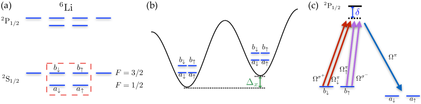
Figure 4: (Color online) Schematics to realize the Hamiltonian $H_{1}$ with cold atoms. (a) Atomic level structure of ${}^{6}\text{Li}$ and the four internal states used to represent the spin and orbital degrees of freedom. (b) The optical lattice is tilted with a homogeneous energy gradient along each direction. (c) Laser configurations to create the first term in $H_{\mathbf{rx}}$. The superscript on each Rabi frequency denotes the polarization of the beam.

V Experimental Implementation and Detection

In this section, we present more details on the implementation scheme with ultracold atoms. In Ref. Wang et al. (2014), an experimental proposal for a three-band chiral TI was put forward. The realization scheme for the four-band Hamiltonian studied here will be similar, with the atomic internal states representing the spin and orbital degrees of freedom. In the previous sections, we studied two Hamiltonians $\mathcal{H}_{1}(\mathbf{k})$ and $\mathcal{H}_{2}(\mathbf{k})$. The latter involves next-nearest-neighbor hopping terms, which will be very challenging for experiment to engineer. In the following, we demonstrate, however, that the implementation of $\mathcal{H}_{1}(\mathbf{k})$ is possible with current technologies. $\mathcal{H}_{1}(\mathbf{k})$ supports topological phases with index $\Gamma=0,1,-2$. It would be very exciting if experiment could simulate $\mathcal{H}_{1}(\mathbf{k})$ and probe its nontrivial topological properties via magneto-electric polarization.

The Hamiltonian $\mathcal{H}_{1}(\mathbf{k})$ was written in momentum space in Sec. II. The real space equivalent can be expressed as (for simplicity, we take $h=0$, $\delta=0$.)

$$H_{1} =\sum_{\mathbf{r}}H_{\mathbf{rx}}+H_{\mathbf{ry}}+H_{\mathbf{rz}},$$ (12)

$$H_{\mathbf{rx}} =-i/2\left(a^{\dagger}_{\uparrow,\mathbf{r+x}}+a^{\dagger}_{\downarrow,\mathbf{r+x}}\right)\left(b_{\uparrow,\mathbf{r}}+b_{\downarrow,\mathbf{r}}\right)$$

$$-i/2\left(a^{\dagger}_{\uparrow,\mathbf{r-x}}-a^{\dagger}_{\downarrow,\mathbf{r-x}}\right)\left(b_{\uparrow,\mathbf{r}}-b_{\downarrow,\mathbf{r}}\right)+\text{H.c.},$$

$$H_{\mathbf{ry}} =-i/2\left(a^{\dagger}_{\uparrow,\mathbf{r+y}}+ia^{\dagger}_{\downarrow,\mathbf{r+y}}\right)\left(b_{\uparrow,\mathbf{r}}-ib_{\downarrow,\mathbf{r}}\right)$$

$$-i/2\left(a^{\dagger}_{\uparrow,\mathbf{r-y}}-ia^{\dagger}_{\downarrow,\mathbf{r-y}}\right)\left(b_{\uparrow,\mathbf{r}}+ib_{\downarrow,\mathbf{r}}\right)+\text{H.c.},$$

$$H_{\mathbf{rz}} =-ia^{\dagger}_{\uparrow,\mathbf{r+z}}b_{\uparrow,\mathbf{r}}-ia^{\dagger}_{\downarrow,\mathbf{r-z}}b_{\downarrow,\mathbf{r}}+\text{H.c.}$$

where $\mathbf{x,y,z}$ represents a unit vector along the $x,y,z$-direction of the cubic lattice, and $a_{\sigma,\mathbf{r}}$ $(b_{\sigma,\mathbf{r}})$ denotes the annihilation operator of the fermionic mode at the $a$ $(b)$ orbital and site $\mathbf{r}$ with the spin state $\sigma$. Basically, all terms in the Hamiltonian are some spin superpositions from one orbital hopping to another orbital. In the following, we take the fermionic species ${}^{6}\text{Li}$, for instance, to illustrate the implementation scheme. Other fermionic atoms can also be used with suitable atomic levels. We make use of four internal states of the hyperfine ground state manifold to carry two pseudospins and two orbitals as depicted in Fig. 4(a). On top of the cubic optical lattice, a linear tilt is assumed along each direction to break the left-right symmetry as does the Hamiltonian [Fig. 4(b)]. This linear tilt can be accomplished with the natural gravitational field, the magnetic field gradient, or the gradient of a dc- or ac-Stark shift Jaksch and Zoller (2003); Aidelsburger et al. (2013); Miyake et al. (2013); Wang et al. (2014). The hopping between orbitals can be activated by two-photon Raman transitions. Here, we show how to get the first term in the Hamiltonian $H_{\mathbf{rx}}$, which is $-i/2(a^{\dagger}_{\uparrow,\mathbf{r+x}}+a^{\dagger}_{\downarrow,\mathbf{r+x}})\left(b_{\uparrow,\mathbf{r}}+b_{\downarrow,\mathbf{r}}\right)$. Every other terms are of similar forms and can be likewise laser-induced. We may decompose it to four separate hoppings from $b$ states at site $\mathbf{r}$ to $a$ states at site $\mathbf{r+x}$. As shown in Fig. 4(c), each of the hopping terms can be induced by a Raman pair:

$$(\Omega_{\uparrow}^{\pi},\Omega^{\pi}) \rightarrow-\tfrac{i}{2}\,a^{\dagger}_{\uparrow,\mathbf{r+x}}b_{\uparrow,\mathbf{r}},\;(\Omega^{\sigma^{-}},\Omega^{\pi}) \rightarrow-\tfrac{i}{2}\,a^{\dagger}_{\downarrow,\mathbf{r+x}}b_{\uparrow,\mathbf{r}}$$

$$(\Omega^{\sigma^{+}},\Omega^{\pi}) \rightarrow-\tfrac{i}{2}\,a^{\dagger}_{\uparrow,\mathbf{r+x}}b_{\downarrow,\mathbf{r}},\;(\Omega^{\pi}_{\downarrow},\Omega^{\pi}) \rightarrow-\tfrac{i}{2}\,a^{\dagger}_{\downarrow,\mathbf{r+x}}b_{\downarrow,\mathbf{r}}$$

The superscript on each Rabi frequency denotes the polarization of the respective beam. The relative phase and amplitude of the hoppings can be controlled by the laser beams. We have four free parameters here, $\Omega_{\uparrow}^{\pi},\Omega^{\sigma^{-}},\Omega^{\sigma^{+}},\Omega^{\pi}_{\downarrow}$, each of which can be adjusted individually to yield the required configuration. These degrees of freedom ensure all other terms in the Hamiltonian can be produced in a similar way. One important aspect we need to be careful is that no spurious terms will be generated with undesired laser coupling. This is guaranteed by energy matching and polarization selection rules. In the undressed atomic basis, all four internal states are at different energies (split by a magnetic field for example), so the four beams coupling $b$ states to the excited states will not interfere with each other. In addition, the different detunings along each direction, $\Delta_{x,y,z}$, preempt the interference of beams that induce hoppings along different directions. There will be, however, some onsite spin-flipping terms induced by the laser beams, but those can be explicitly compensated by some r.f. fields.

The above scheme is hence able to engineer the Hamiltonian $H_{1}$ and is feasible with current technologies. The actual experiment will be challenging since many laser beams are involved with careful detunings. Nonetheless, all these beams can be drawn from the same laser with small frequency shifts produced by an acoustic or electric optical modulator. The uniform orbital magnetic field required to observe the topological polarization can be imprinted from the phase of the laser beams as an artificial gauge field Jaksch and Zoller (2003); Aidelsburger et al. (2013); Miyake et al. (2013); Wang et al. (2014). Lastly, the gap opening term in Eq. (9) can be created by extra laser beams focused on the surfaces, producing an effective Zeeman splitting. Other gap opening mechanisms on the surface should also work since the magneto-electric polarization is a bulk effect. The accumulated charge will be detectable from atomic density measurements Nelson et al. (2007); Bakr et al. (2010); Sherson et al. (2010); Deng et al. (2014b). Note that the density measurements do not need to be restricted to the surfaces, as a measurement for half of the sample produces good results, as shown in Fig. 3. One half of the sample can be removed to another state by shining a laser beam. The density on the other half of the sample can in turn be measured by time-of-flight imaging Deng et al. (2014b). As we have demonstrated in the previous section, the charge quantization is very robust to perturbations, so any weak perturbations introduced to the Hamiltonian, even those breaking the chiral symmetry in the bulk, should not alter detection results.

VI Conclusions

In summary, we study the $\mathbb{Z}$ character of chiral topological insulators by simulating the quantized magneto-electric effect of a nontrivial phase. We show that the $\mathbb{Z}$ character, not only the $\mathbb{Z}_{2}$ part, can be observed through magneto-electric polarization by properly gapping the system. An experimental scheme is also proposed for implementation and detection with cold atoms. This demonstrates explicitly how the topological invariant appears in physical observables for chiral TIs and will be important for experimental characterization.

Appendix A Bulk-edge correspondence

The bulk edge correspondence tells us that the bulk topological index should have a surface manifestation, typically through the number of gapless Dirac cones on the surface. This is generally verified for lower topological index, such as 1 or 2. By imposing an open boundary condition along the $z$ direction for chiral topological insulators of different index, we find that the winding number corresponds to the total number of Dirac cones counted for all inequivalent surface states (i.e. not counting degeneracies).

Following Ref. Deng et al. (2014a) to take a quaternion power $n$, we can generalize the Hamiltonians in the main text from $\mathcal{H}_{1}(\mathbf{k})$ and $\mathcal{H}_{2}(\mathbf{k})$ to $\mathcal{H}_{n}(\mathbf{k})$. For the Hamiltonian $\mathcal{H}_{1}(\mathbf{k})$ (i.e. $n=1$), when $h=2$, the winding number $\Gamma=1$ guarantees the existence of 1 Dirac cone [Fig. 5(a)]. For the Hamiltonian $\mathcal{H}_{2}(\mathbf{k})$ (i.e. $n=2$), when $h=0$, the winding number is $\Gamma=4$. So there are two inequivalent surface states on each surface with two Dirac cones each [Fig. 5(b)]. In general, we have $m$ inequivalent surface states with 1 Dirac cone each for $n=m,1<|h|<3,\Gamma=m$, and $m$ inequivalent surface states with 2 Dirac cones each for $n=m,-1<h<1,\Gamma=2m$. These have been explicitly verified up to $n=3$. Hence, the winding number $\Gamma$ does correspond to the total number of Dirac cones for all inequivalent surface states.

(a)

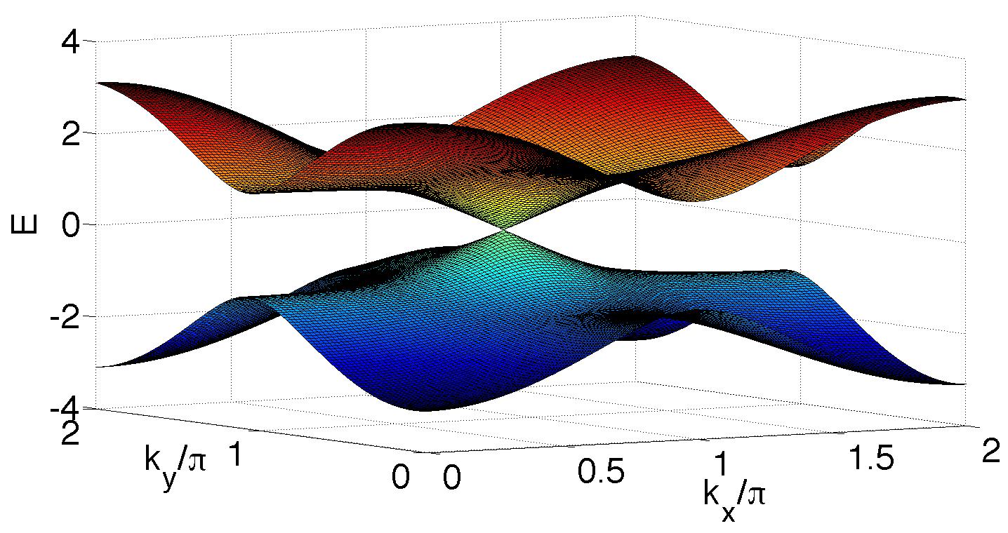
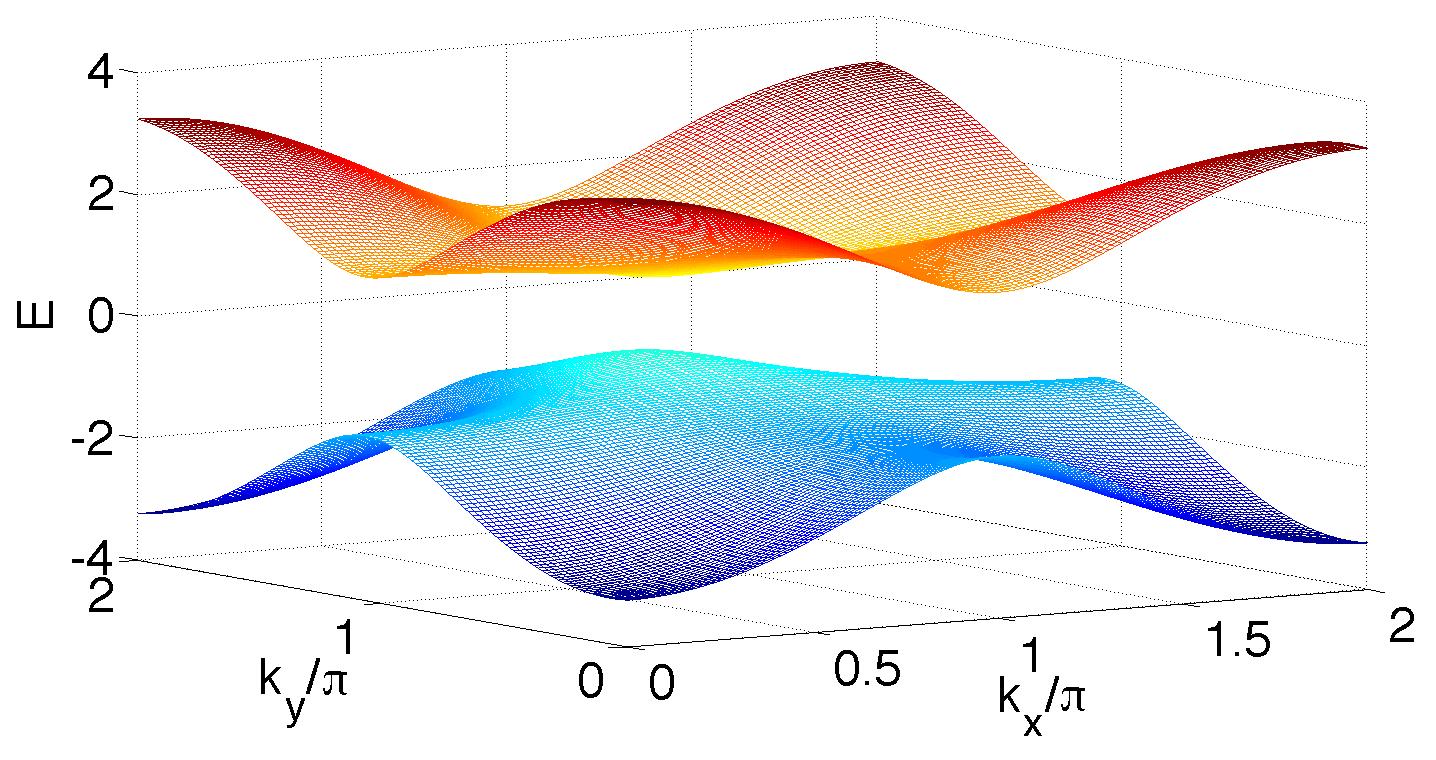
(b)

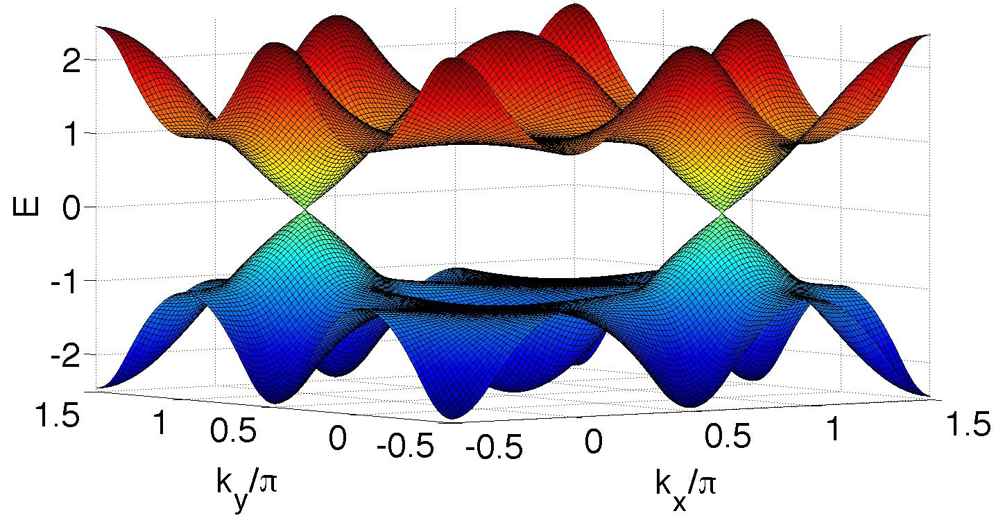
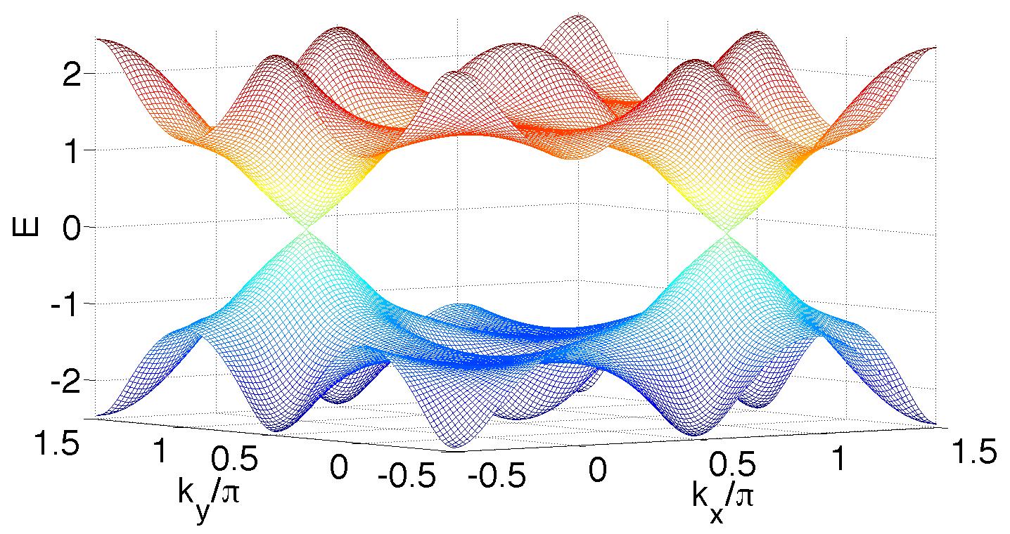
Figure 5: (Color online) Spectrum for the surface states showing the number of Dirac cones. The upper panels in (a) and (b) show the lowest conduction and highest valence band. The lower panels show the next two bands closest to the Fermi energy. (a) For $\mathcal{H}_{1}(\mathbf{k})$, $h=2,\delta=0.5$ with winding number $\Gamma=1$ and 1 Dirac cone. (b) For $\mathcal{H}_{2}(\mathbf{k})$, $h=0,\delta=0$ with winding number $\Gamma=4$ and 4 Dirac cones in total. The $\Gamma$ point is displaced from the center for better display of the Dirac cones.

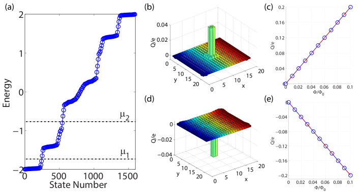
Figure 6: (Color online) (a) Energy spectrum for the one-layer Hamiltonian $\mathcal{H}_{1}(\mathbf{k})$ with a strong uniform magnetic field and unit cell flux as $\frac{1}{3}\Phi_{0}$. An additional weak flux tube is inserted through the center lattice cell of the layer, with flux up to $\Phi/\Phi_{0}=0.1$. (b) and (c) [(d) and (e)] correspond to the charge polarization with respect to the increasing flux tube at a chemical potential $\mu_{1}$ [$\mu_{2}$]. Charge is accumulated around the flux tube, and by changing the chemical potential and hence the Landau level occupancy, the charge accumulation rate can be modified by an integer.

Appendix B Surface orbital field and integer quantum Hall layers

The $2\pi$ periodicity of the $\theta$ term is mathematically related to the gauge freedom in the low-energy effective field theory. Physically, it is associated with the freedom to coat an integer quantum Hall layer on the surface, or equivalently to change the chemical potential and hence the Landau level occupancy of the surface in an orbital magnetic field. Here, we numerically verify this physical intuition. To do that, we consider a single layer of the Hamiltonian $\mathcal{H}_{1}(\mathbf{k})$, so the $z$ component drops out. A strong uniform orbital field is added to the layer via Peierls substitution with the Landau gauge $\mathbf{A}=Bx\hat{y}$. $Ba^{2}=\frac{1}{3}\Phi_{0}$, where $a$ is the lattice constant, and $\Phi_{0}$ is the flux quantum. For the Hofstadter Hamiltonian, this strong orbital field will produce three gapped Landau levels. Here, a similar structure is developed as shown in Fig. 6(a). There are six bands with the middle two bands gapless. The extra number of bands are due to the spin and orbital degrees of freedom. On top of the strong uniform magnetic field, an additional weak flux tube is inserted through the center lattice. By Laughlin’s flux insertion argument, the charge accumulated around the flux tube should be $Q/e=C\Phi/\Phi_{0}$, where $C$ is the Chern number being an integer. Figures 6(b) and 6(c) [6(d) and 6(e)] show the charge polarization at a chemical potential $\mu_{1}$ [$\mu_{2}$]. From the slope, we infer that the first band has a Chern number $C=2$ and the second band has a Chern number $C=-4$. So by changing the surface chemical potential, we could modify the charge accumulation rate by an integer. Alternatively, in the absence of this strong orbital magnetic field, with a surface gapping term $H_{S}$ in Eq. (9) of the main text, there is only one gap and no such integer quantum Hall layers. Therefore the $\mathbb{Z}$ character of the winding number can be observed through such integrally quantized magneto-electric polarization measurements.

References

- Schnyder et al. (2008) A. P. Schnyder, S. Ryu, A. Furusaki, and A. W. W. Ludwig, Phys. Rev. B 78, 195125 (2008).
- Kitaev (2009) A. Kitaev, in AIP Conf. Proc., Vol. 1134 (2009) p. 22.
- Hasan and Kane (2010) M. Z. Hasan and C. L. Kane, Rev. Mod. Phys. 82, 3045 (2010).
- Moore (2010) J. E. Moore, Nature 464, 194 (2010).
- Qi and Zhang (2011) X.-L. Qi and S.-C. Zhang, Rev. Mod. Phys. 83, 1057 (2011).
- Kane and Mele (2005) C. L. Kane and E. J. Mele, Phys. Rev. Lett. 95, 146802 (2005).
- Bernevig et al. (2006) B. A. Bernevig, T. L. Hughes, and S.-C. Zhang, Science 314, 1757 (2006).
- Fu et al. (2007) L. Fu, C. L. Kane, and E. J. Mele, Phys. Rev. Lett. 98, 106803 (2007).
- Thouless et al. (1982) D. J. Thouless, M. Kohmoto, M. P. Nightingale, and M. Den Nijs, Phys. Rev. Lett. 49, 405 (1982).
- Qi et al. (2008) X.-L. Qi, T. L. Hughes, and S.-C. Zhang, Phys. Rev. B 78, 195424 (2008).
- Essin et al. (2009) A. M. Essin, J. E. Moore, and D. Vanderbilt, Phys. Rev. Lett. 102, 146805 (2009).
- Hosur et al. (2010) P. Hosur, S. Ryu, and A. Vishwanath, Phys. Rev. B 81, 045120 (2010).
- Ryu et al. (2010) S. Ryu, A. P. Schnyder, A. Furusaki, and A. W. W. Ludwig, New J. Phys. 12, 065010 (2010).
- Lewenstein et al. (2007) M. Lewenstein, A. Sanpera, V. Ahufinger, B. Damski, A. Sen De, and U. Sen, Adv. Phys. 56, 243 (2007).
- Dalibard et al. (2011) J. Dalibard, F. Gerbier, G. Juzeliūnas, and P. Öhberg, Rev. Mod. Phys. 83, 1523 (2011).
- Goldman et al. (2014) N. Goldman, G. Juzeliūnas, P. Öhberg, and I. B. Spielman, Rep. Prog. Phys. 77, 126401 (2014).
- Wang et al. (2014) S.-T. Wang, D.-L. Deng, and L.-M. Duan, Phys. Rev. Lett. 113, 033002 (2014).
- Shiozaki and Fujimoto (2013) K. Shiozaki and S. Fujimoto, Phys. Rev. Lett. 110, 076804 (2013).
- Jaksch and Zoller (2003) D. Jaksch and P. Zoller, New J. Phys. 5, 56 (2003).
- Aidelsburger et al. (2013) M. Aidelsburger, M. Atala, M. Lohse, J. T. Barreiro, B. Paredes, and I. Bloch, Phys. Rev. Lett. 111, 185301 (2013).
- Miyake et al. (2013) H. Miyake, G. A. Siviloglou, C. J. Kennedy, W. C. Burton, and W. Ketterle, Phys. Rev. Lett. 111, 185302 (2013).
- Deng et al. (2014a) D.-L. Deng, S.-T. Wang, and L.-M. Duan, Phys. Rev. B 89, 075126 (2014a).
- Stamper-Kurn et al. (1999) D. M. Stamper-Kurn, A. P. Chikkatur, A. Görlitz, S. Inouye, S. Gupta, D. E. Pritchard, and W. Ketterle, Phys. Rev. Lett. 83, 2876 (1999).
- Zhu et al. (2007) S.-L. Zhu, B. Wang, and L.-M. Duan, Phys. Rev. Lett. 98, 260402 (2007).
- Laughlin (1981) R. B. Laughlin, Phys. Rev. B 23, 5632 (1981).
- Rosenberg et al. (2010) G. Rosenberg, H.-M. Guo, and M. Franz, Phys. Rev. B 82, 041104 (2010).
- Chang et al. (2013) C.-Z. Chang, J. Zhang, X. Feng, J. Shen, Z. Zhang, M. Guo, K. Li, Y. Ou, P. Wei, L.-L. Wang, Z.-Q. Ji, Y. Feng, S. Ji, X. Chen, J. Jia, X. Dai, Z. Fang, S.-C. Zhang, K. He, Y. Wang, L. Lu, X.-C. Ma, and Q.-K. Xue, Science 340, 167 (2013).
- Essin et al. (2010) A. M. Essin, A. M. Turner, J. E. Moore, and D. Vanderbilt, Phys. Rev. B 81, 205104 (2010).
- Nelson et al. (2007) K. D. Nelson, X. Li, and D. S. Weiss, Nat. Phys. 3, 556 (2007).
- Bakr et al. (2010) W. S. Bakr, A. Peng, M. E. Tai, R. Ma, J. Simon, J. I. Gillen, S. Foelling, L. Pollet, and M. Greiner, Science 329, 547 (2010).
- Sherson et al. (2010) J. F. Sherson, C. Weitenberg, M. Endres, M. Cheneau, I. Bloch, and S. Kuhr, Nature 467, 68 (2010).
- Deng et al. (2014b) D.-L. Deng, S.-T. Wang, and L.-M. Duan, Phys. Rev. A 90, 041601(R) (2014b).