Efficient computation of highly oscillatory integrals by using QTT tensor approximation

Abstract

We propose a new method for the efficient approximation of a class of highly oscillatory weighted integrals where the oscillatory function depends on the frequency parameter $\omega\geq 0$, typically varying in a large interval. Our approach is based, for fixed but arbitrary oscillator, on the pre-computation and low-parametric approximation of certain $\omega$-dependent prototype functions whose evaluation leads in a straightforward way to recover the target integral. The difficulty that arises is that these prototype functions consist of oscillatory integrals which makes them difficult to evaluate. Furthermore they have to be approximated typically in large intervals. Here we use the quantized-tensor train (QTT) approximation method for functional $m$-vectors of logarithmic complexity in $m$ in combination with a cross-approximation scheme for TT tensors. This allows the accurate approximation and efficient storage of these functions in the wide range of grid and frequency parameters. Numerical examples illustrate the efficiency of the QTT-based numerical integration scheme on various examples in one and several spatial dimensions.

AMS subject classifications: 65F30, 65F50, 65N35, 65D30

Keywords: highly oscillatory integrals, quadrature, tensor representation, QTT tensor approximation.

1 Introduction and Problem Setting

In this paper we are interested in the efficient approximation of (highly) oscillatory integrals. In the most general setting these integrals are of the form

$$\int_{\Omega}f(x)h_{\omega}(x)dx,$$ (1.1)

where $\Omega\subset\mathbb{R}^{d}$, $d\in\mathbb{N}$, is a general open domain, $h_{\omega}$ is an oscillatory function where the parameter $\omega\geq 0$ determines the rate of oscillation and $f$ is a non-oscillatory (typically analytic) function. An important special case occurs if the oscillatory function is the imaginary exponential function with oscillator $g$, i.e.,

$$h_{\omega}(x)=\operatorname{e}^{\operatorname{i}\omega g(x)}.$$ (1.2)

This type of oscillatory integrals has been in the main focus of research in recent years since they play an important role in a wide range of applications. Prominent examples include the solution of highly oscillatory differential equations via the modified Magnus expansion (see [12, 9]), boundary integral formulations of the Helmholtz equation [19], the evaluation of special functions and orthogonal expansions (e.g. Fourier series, modified Fourier series) (see [15]), lattice summation techniques and ODEs/PDEs with oscillating and quasi-periodic coefficients [17, 18, 23].

Other types of oscillatory functions that can be found in the literature include the Bessel oscillator $h_{\omega}(x)=J_{\nu}(\omega x)$ (see [36]) and functions of the form $h_{\omega}(x)=v(\sin(\omega\theta(x)))$ (see [13]), as well as some examples considered in [31].

For $d=1$ an obvious way to obtain an approximation of (1.1) is Gaussian quadrature. For large $\omega$ however such standard approaches become ineffective since the number of quadrature points has to be chosen proportional to $\omega$ in order to resolve the oscillations of the integrand. Therefore several alternative approaches have been developed to overcome this difficulty. The most successful methods include the asymptotic expansion, Filon-type methods, Levin-type methods and numerical steepest descent (see e.g. [26, 14, 16, 10, 11, 25]) and recently introduced Gaussian quadrature rules with complex weight functions (see [2, 1]). Although these methods are mathematically elegant they can typically not be applied in a “black-box” fashion since either derivatives of $f$ and $g$ are involved, moments $\int_{a}^{b}x^{k}\operatorname{e}^{\operatorname{i}\omega g(x)}$ must be known or computations in the complex plane have to be performed. Furthermore these methods get more complicated (or even non-applicable) if the oscillator $g$ has stationary points (i.e. points where $g^{\prime}(x)$ vanishes), multidimensional integrals are considered or $f$ and $g$ are not analytic. For general oscillators $h_{\omega}(x)$ it is typically not known how these methods can be applied (see however [36, 13]).

In this paper we propose a Filon-like method which is based, for fixed but arbitrary oscillators $g$ or $h_{\omega}$ respectively, on the pre-computation and approximation of certain $\omega$-dependent prototype functions whose evaluation leads in a straightforward way to approximations of (1.1). The difficulty that arises is that these prototype functions consist of oscillatory integrals which makes them difficult to evaluate. Furthermore they have to be approximated typically in large intervals. Here we use the quantized-tensor train (QTT) approximation method for functional $M$-vectors [20, 21] of logarithmic complexity in $M$ in combination with a cross-approximation scheme for TT tensors introduced in [27]. This allows the accurate approximation and efficient storage of these functions in the wide range of grid and frequency parameters. Literature surveys on tensor methods can be found in [24, 22, 8, 7, 23, 3].

The QTT approximation applies to the quantized image of the target discrete function, obtained by its isometric folding transformation to the higher dimensional quantized tensor space. For example, a vector of size $M=2^{L}$ can be successively reshaped by a diadic folding to an $L$-fold tensor in $\bigotimes_{j=1}^{L}\mathbb{R}^{2}$ of the irreducible mode size $m=2$ (quantum of information), then the low-rank approximation in the canonical or TT format can be applied consequently. The rigorous justification of the QTT approximation method for rather general classes of functional vectors was first presented in [20]. For our particular application in this paper the most important result is the existance of rank-$1$ QTT representation of the complex exponential $M$-vector $\{e^{i\omega n}\}_{n=0}^{M-1}$. The QTT-type representation for $2^{L}\times 2^{L}$ matrices was introduced in [28], see survey papers [22, 23] for further references on the topic.

The quadrature scheme proposed in this article does not require analytic knowledge about $f,g$ or $h_{\omega}$ respectively and can therefore be applied in a black-box fashion. One condition for its efficiency is that $f$ can be well approximated by polynomials which is typically the case for analytic, non-oscillatory functions. The quadrature error of the method can be easily estimated and controlled in terms of $f$. Furthermore the method is uniformly accurate for all considered $\omega$.

Since it is the most important case in practice we carry out the description and the analysis of our scheme only for the case (1.2). We emphasize, however, that the method can be easily applied also to the more general situation (1.1) (see Section 5). We introduce the notation

$$I(\omega,f):=\int_{\Omega}f(x)\operatorname{e}^{\operatorname{i}\omega g(x)}dx.$$ (1.3)

We consider the oscillator $g$ and the domain $\Omega$ to be arbitrary but fixed and are interested in the efficient computation of (1.3) for different real-valued functions $f$ and different values of $\omega$. Without loss of generality we assume from now on that $|g(x)|\leq 1$ for all $x\in\Omega$. A separation of the real- and imaginary part of $I(\omega,f)$ leads to the integrals

$$I_{\mathscr{R}}(\omega,f):=\int_{\Omega}f(x)\cos(\omega g(x))dx,\quad I_{\mathscr{I}}(\omega,f):=\int_{\Omega}f(x)\sin(\omega g(x))dx$$

which will be considered in the following.

The remainder of the paper is structured as follows. Section 2 recalls the main ideas of the QTT approximation of functional vectors. The central Section 3 presents the basic QTT approximation scheme for the fast computation of one- and multidimensional oscillating integrals. Section 4 describes and theoretically analyzes the QTT tensor approximation of special functions of interest, while Section 5 presents the numerical illustrations.

2 Quantized-TT approximation of functional vectors

A real tensor of order $d$ is defined as an element of finite dimensional Hilbert space $\mathbb{W}_{\bf m}=\bigotimes_{\ell=1}^{d}X_{\ell}$ of the $d$-fold, $M_{1}\times...\times M_{d}$ real-valued arrays, where $X_{\ell}=\mathbb{R}^{M_{\ell}}$ and ${\bf m}=(M_{1},\ldots,M_{d})$. A tensor $\textsf{{A}}\in\mathbb{R}^{\cal I}$ with ${\cal I}=I_{1}\times...\times I_{d}$, can be represented entrywise by

$$\textsf{{A}}=[\textsf{A}(i_{1},...,i_{d})]\equiv[\textsf{A}_{i_{1},...,i_{d}}]\quad\mbox{with}\quad i_{\ell}\in I_{\ell}:=\{1,...,M_{\ell}\}.$$

The Euclidean scalar product, $\left\langle\cdot,\cdot\right\rangle:\mathbb{W}_{\bf m}\times\mathbb{W}_{\bf m}\to\mathbb{R}$, is defined by

$$\left\langle\textsf{{A}},\textsf{{B}}\right\rangle:=\sum_{{\bf i}\in{\cal I}}\textsf{A}({\bf i})\textsf{B}({\bf i}),\quad\textsf{{A}},\textsf{{B}}\in\mathbb{W}_{\bf m}.$$

The storage size for a $d$th order tensor scales exponentially in $d$, $\operatorname{dim}(\mathbb{W}_{{\bf m}})=M_{1}\cdots M_{d}$ (the so-called "curse of dimensionality"). For ease of presentation we further assume that $M_{\ell}=M$ for $\ell=1,...,d$.

The efficient low-parametric representations of $d$th order tensors can be realized by using low-rank separable decompositions (formats). The commonly used canonical and Tucker tensor formats [24] are constructed by combination of the simplest separable elements given by rank-$1$ tensors,

$$\textsf{{A}}=\bigotimes_{\ell=1}^{d}\textsf{A}^{(\ell)},\quad\textsf{A}^{(\ell)}\in\mathbb{R}^{M},$$

which can be stored with $dM$ numbers.

In this paper we apply the factorized representation of $d$th order tensors in the tensor train (TT) format [30], which is the particular case of the so called matrix product states (MPS) decomposition. The latter was introduced since longer in the physics community and successfully applied in quantum chemistry computations and in spin systems modeling [35, 34, 33].

For a given rank parameter ${\bf r}=(r_{0},...,r_{d})$, and the respective index sets $J_{\ell}=\{1,...,r_{\ell}\}$ ($\ell=0,1,...,d$), with the constraint $J_{0}=J_{d}=\{1\}$ (i.e., $r_{0}=r_{d}=1$), the rank-${\bf r}$ TT format contains all elements $\textsf{{A}}=[\textsf{A}(i_{1},...,i_{d})]\in\mathbb{W}_{\bf m}$ which can be represented as the contracted products of $3$-tensors over the $d$-fold product index set ${\cal J}:=\times_{\ell=1}^{d}J_{\ell}$, such that

$$\textsf{{A}}=\sum\limits_{{\bf\alpha}\in{\cal J}}\textsf{A}^{(1)}_{1,\alpha_{1}}\otimes\textsf{A}^{(2)}_{\alpha_{1},\alpha_{2}}\otimes\cdots\otimes\textsf{A}^{(d)}_{\alpha_{d-1},1},$$

where $\textsf{A}^{(\ell)}_{\alpha_{\ell-1},\alpha_{\ell}}\in\mathbb{R}^{M}$, ($\ell=1,...,d$), and $\textsf{A}^{(\ell)}=[\textsf{A}^{(\ell)}_{\alpha_{\ell-1},\alpha_{\ell}}]$ is the vector-valued $r_{\ell-1}\times r_{\ell}$ matrix ($3$-tensor). The TT representation reduces the storage cost to $O(dr^{2}M)$, $r=\max{r_{\ell}}$.

In the case of large mode size, the asymptotic storage for a $d$th order tensor can be reduced to logarithmic scale $O(d\log M)$ by using quantics-TT (QTT) tensor approximation [20, 21]. In our paper we apply this approximation techniques to long $M$-vectors generated by sampling certain highly-oscillating functions on the uniform grid.

The QTT-type approximation of an $M$-vector with $M=q^{L}$, $L\in\mathbb{N}$, $q=2,3,...$, is defined as the tensor decomposition (approximation) in the canonical, TT or some related format applied to a tensor obtained by the folding (reshaping) of the initial long vector to an $L$-dimensional $q\times\ldots\times q$ data array that is thought as an element of the quantized tensor space $\mathbb{Q}_{{q},L}=\bigotimes_{j=1}^{L}\mathbb{K}^{q},\;\mathbb{K}\in\{\mathbb{R},\mathbb{C}\}$. A vector $X=[X(i)]_{i\in I}\in\mathbb{W}_{{M}},$ is reshaped to its quantics image in $\mathbb{Q}_{q,L}$ by $q$-adic folding,

$$\mathcal{F}_{q,L}:X\to\textsf{{Y}}=[Y({\bf j})]\in\mathbb{Q}_{q,L},\quad{\bf j}=\{j_{1},\ldots,j_{L}\},$$

with $j_{\nu}\in\{1,2\}$ for $\nu=1,...,L$, where for fixed $i$, we have $Y({\bf j}):=X(i)$, and $j_{\nu}=j_{\nu}(i)$ is defined via $q$-coding, $j_{\nu}-1=C_{-1+\nu},$ such that the coefficients $C_{-1+\nu}$ are found from the $q$-adic representation of $i-1$ (binary coding for $q=2$),

$$i-1=C_{0}+C_{1}q^{1}+\cdots+C_{L-1}q^{L-1}\equiv\sum\limits_{\nu=1}^{L}(j_{\nu}-1)q^{\nu-1}.$$

Assuming that for the rank-${\bf r}$-TT approximation of the quantics image Y we have $r_{k}\leq r$, $k=1,\ldots,L$, then the complexity of this tensor representation is reduced to the logarithmic scale

$$qr^{2}\log_{q}M\ll M.$$

The computational gain of the QTT approximation is justified by the perfect rank decomposition proven in [21] for a wide class of function-related tensors obtained by sampling the corresponding functions over a uniform or properly refined grid. In particular, this class of functions includes complex exponentials, trigonometric functions, polynomials and Chebyshev polynomials, wavelet basis functions (see also [6, 29, 17] for further results on QTT approximation).

The low-rank QTT approximation can be also proven for Gaussians, as well as for the 3D Newton, Yukawa and Helmholtz kernels.

In the following we apply the QTT approximation method to the problem of fast integration of highly oscillating functions introduced in the introduction.

3 Approximation procedure

3.1 One-dimensional integrals

For simplicity we introduce the general idea of the approximation at first for one dimensional integrals of the form

$$I_{\mathscr{R}}(\omega,f):=\int_{-1}^{1}f(x)\cos(\omega g(x))dx.$$ (3.1)

The case $I_{\mathscr{I}}(\omega,f):=\int_{-1}^{1}f(x)\sin(\omega g(x))dx$ and integrals over arbitrary intervals $[a,b]$ will not be treated separately since the procedure is completely analogous (after a suitable transformation to the interval $[-1,1]$). Recall that we are interested in the computation of integrals of the form (3.1) for different functions $f$ and different frequencies $\omega$, hence the notation $I_{\mathscr{R}}(\omega,f)$.
In the following we assume that $f$ is a smooth nonoscillatory function that can be well approximated by polynomials of degree $N$. We introduce the Chebyshev polynomials by

$$T_{0}(x) =1,\quad T_{1}(x)=x,$$

$$T_{n+1}(x) =2xT_{n}(x)-T_{n-1}(x)\quad n=1,2,\ldots$$

and seek an approximation of $f$ of the form

$$f_{N}(x)=\sum_{k=0}^{N}c_{k}T_{k}(x),$$ (3.2)

where $f_{N}$ interpolates $f$ in the Chebyshev-Gauss-Lobatto points

$$x_{k}=\cos\left(\frac{k\pi}{N}\right)\quad 0\leq k\leq N.$$

In this case the coefficients $c_{k}$ in (3.2) are given by

$$c_{k}=\frac{1}{\alpha_{k}N}\sum_{j=0}^{2N-1}f\left(\cos\left(\frac{j\pi}{N}\right)\right)\cos\left(\frac{kj\pi}{N}\right),\quad k=0,\ldots,N,$$

where

$$\alpha_{0}=\alpha_{N}=2,\alpha_{k}=1\quad\text{for}\quad 1\leq k\leq N-1.$$

The coefficients $c_{k}$ can be computed efficiently in $O(N\log N)$ operations using fast cosine transform methods. Recall that this polynomial approximation converges exponentially in $N$ if $f$ is sufficiently smooth. This is summarized in the following proposition.

Proposition 3.1.

Let $f$ be analytic in the Bernstein regularity ellipse

$$\mathcal{E}_{\rho}:=\left\{w\in\mathbb{C}:|w-1|+|w+1|\leq\rho+\rho^{-1}\right\},$$

with $\rho>1$. Furthermore let $|f(x)|\leq M_{0}$ in $\mathcal{E}_{\rho}$ for some $M_{0}>0$. Then the Chebyshev interpolant $f_{N}$ in (3.2) satisfies

$$\|f-f_{N}\|_{\infty}\leq\frac{4M_{0}}{\rho-1}\rho^{-N},\quad N\in\mathbb{N}_{0}.$$

Proof.

See [32]. ∎

We obtain an approximation of $I_{\mathscr{R}}(\omega,f)$ by replacing $f$ by $f_{N}$ and computing $I_{\mathscr{R}}(\omega,f_{N})$ (see also [5, 4, 37], where this approach is refered to as Filon-Clenshaw-Curtis quadrature rule). The corresponding error can be easily estimated in terms of the error of the Chebyshev interpolation of $f$. It holds

$$\left|I_{\mathscr{R}}(\omega,f)-I_{\mathscr{R}}(\omega,f_{N})\right| =\left|\int_{-1}^{1}\left(f(x)-f_{N}(x)\right)\cos(\omega g(x))dx\right|$$

$$\leq\|f-f_{N}\|_{\infty}\int_{-1}^{1}|\cos(\omega g(x))|dx$$

$$\leq 2\|f-f_{N}\|_{\infty}.$$

Under the assumptions of Proposition 3.1 we therefore have

$$\left|I_{\mathscr{R}}(\omega,f)-I_{\mathscr{R}}(\omega,f_{N})\right|\leq\frac{8M_{0}}{\rho-1}\rho^{-N},\quad N\in\mathbb{N}_{0},$$ (3.3)

i.e., exponential convergence of $I_{\mathscr{R}}(\omega,f_{N})$ to the exact value with respect to $N$. Obviously this is also true for $I_{\mathscr{I}}(\omega,f)$. Note that the asymptotic order of this method is $\mathcal{O}(\omega^{2})$ since $f_{N}$ interpolates $f$ in the endpoints of the interval.

Remark 3.2.

In the following $f_{N}$ could also be written in the equivalent form

$$f_{N}(x)=\sum_{k=0}^{N}f(x_{k})L_{k}(x),$$ (3.4)

where

$$L_{k}(x)=\prod_{\nu=0,\nu\neq k}^{N}\frac{x-x_{\nu}}{x_{k}-x_{\nu}}$$

are the corresponding Lagrange polynomials. This representation has the advantage that the Chebyshev coefficient do not have to be computed. While the analysis of the scheme in Section 4 assumes $f_{N}$ to be in the form (3.2), the numerical experiments (see Section 5) indicate that the results are very similar. In Section 3.2 we will make use of (3.4).

We now turn to the question how to compute $I_{\mathscr{R}}(\omega,f_{N})$ efficiently. Since $f_{N}$ is supposed to approximate $f$ accurately this task is in general not easier than the original problem although $f_{N}$ is a polynomial. However the approximation of $f$ with Chebyshev polynomials leads to certain prototype functions of integrals that we want to precompute and store in the following. We have

$$I_{\mathscr{R}}(\omega,f_{N}) =\sum_{k=0}^{N}c_{k}\int_{-1}^{1}T_{k}(x)\cos(\omega g(x))dx=\sum_{k=0}^{N}c_{k}\,I_{\mathscr{R}}(\omega,T_{k}).$$ (3.5)

Thus, the question how to evaluate $I_{\mathscr{R}}(\omega,f_{N})$ boils down to the question how to efficiently evaluate $I_{\mathscr{R}}(\omega,T_{k})$ for a certain range of frequencies $\omega\in\left[\omega_{\min},\omega_{\max}\right]$, moderate $k$ (typically $k\leq 12$) and different oscillators $g$. Our goal is to precompute $I_{\mathscr{R}}(\omega,T_{k})$ for fixed $k$ and $g$. Thus the function

$$I_{\mathscr{R}}(\cdot,T_{k}):\left[\omega_{\min},\omega_{\max}\right]\rightarrow\mathbb{R}$$ (3.6)

needs to be accurately represented and stored in order to compute an approximation of $I_{\mathscr{R}}(\omega,f_{N})$ via (3.5). Note that this function needs to be approximated in a possibly large interval $\left[\omega_{\min},\omega_{\max}\right]$. Thus standard techniques like, e.g., polynomial interpolation/approximation are typically not effective (see Figure 3.1). Once the prototype functions $I_{\mathscr{R}}(\cdot,T_{k})$ have been precomputed for different $k$, integrals of the form (3.1) can be easily approximated for different functions $f$ and frequencies $\omega$.

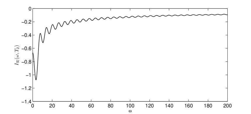
Figure 3.1: Plot of $I_{\mathscr{R}}(\omega,T_{2})$ for $g(x)=x^{2}$.

In the present paper we will represent functions of the form (3.6) on the interval $\left[\omega_{\min},\omega_{\max}\right]$ pointwise on a very fine grid (see Remark 3.3 for a precise statement) via low rank QTT tensor representations that were introduced in the preceding section. The straightforward way to obtain such a representation is to evaluate $I_{\mathscr{R}}(\cdot,T_{k})$ at every point of the grid, to reshape the resulting vector to its quantics image and to approximate the resulting tensor in the TT-format. Since we seek to approximate $I_{\mathscr{R}}(\cdot,T_{k})$ at grids that can easily exceed $2^{40}$ points this strategy is prohibitively expensive. Instead the final QTT tensor can be set up directly without computing the function at every point of the grid. This is achieved using a TT/QTT cross approximation scheme conceptually introduced [27].

It allows the computation of the QTT tensor using only a low number of the original tensor elements, i.e. by evaluating $I_{\mathscr{R}}(\cdot,T_{k})$ only at a few $\omega\in\left[\omega_{\min},\omega_{\max}\right]$. More precisely, the rank-$r$ QTT-cross approximation of a $2^{L}$ tensor calls only $O(Lr^{2})$ entries of the original tensor. Notice that the required accuracy of the QTT approximation is achieved by the adaptive choice of the QTT rank $r$ within the QTT-cross approximation scheme. The required computation of $I_{\mathscr{R}}(\cdot,T_{k})$ at these special points is the most expensive part of the precomputation step since for fixed $\omega$ this is itself an oscillatory integral. Since the overall scheme to approximate (3.1) is supposed to work in a black-box fashion (and we do not want to use specific knowledge about $g$) we suggest to compute $I_{\mathscr{R}}(\omega,T_{k})$ for fixed $\omega$ (within the cross approximation scheme) by standard techniques like composite Gauss-Legendre quadrature. Depending on $\omega$ this certainly requires a high number of subintervals/quadrature points to achieve accurate results but since this has to be done only once in the precomputation step and due to its generality we think that this is a suitable strategy. In Section 5 we show that the time to precompute the QTT tensor is indeed very moderate in practice.

Once the functions $I_{\mathscr{R}}(\omega,T_{k}),\omega\in\left[\omega_{\min},\omega_{\max}\right]$ have been precomputed for $0\leq k\leq N$ and stored in the QTT format we obtain an approximation of $I_{\mathscr{R}}(\omega,f_{N})$ (and therefore $I_{\mathscr{R}}(\omega,f)$) for a specific $\omega$ by evaluating the corresponding entry of the $(N+1)$ different QTT-tensors and combining them according to (3.5) (see Algorithm 1). Since the entry-wise evaluation of a rank-$r$ TT-tensor requires $O(Lr^{2})$ operations, the cost to obtain an approximation of $I_{\mathscr{R}}(\omega,f_{N})$ from the precomputed tensors sums up to $O((N+1)Lr^{2})$ operations which is independent of $\omega$.

Remark 3.3.

With the strategy above the function $I_{\mathscr{R}}(\cdot,T_{k})$ is only represented at discrete grid points. In order to evaluate $I_{\mathscr{R}}(\omega,T_{k})$ at an arbitrary point $\omega_{0}$ in $\left[\omega_{\min},\omega_{\max}\right]$, $\omega_{0}$ first has to be rounded to the nearest grid point. This leads to an additional error in the overall approximation of $I_{\mathscr{R}}(\omega_{0},f)$ which can be easily estimated. We denote by $\tilde{\omega}_{0}$ the grid point that is closest to $\omega_{0}$. A Taylor expansion around $\tilde{\omega}_{0}$ shows that

$$\left|I_{\mathscr{R}}(\tilde{\omega}_{0},f)-I_{\mathscr{R}}(\omega_{0},f)\right|\leq 2\left(\operatorname{e}^{|\tilde{\omega}_{0}-\omega_{0}|}-1\right).$$

If the distance between two sampling points is $h$ the error due to rounding on this grid is therefore at most $2\left(\operatorname{e}^{h/2}-1\right)$. We therefore need $h<2\ln(\varepsilon_{r}/2+1)$ to assure that the error due to rounding does not exceed $\varepsilon_{r}$. In practice $2^{30}-2^{40}$ grid points are typically sufficient to keep the error due to rounding negligible. It becomes evident in Section 5 that the QTT approximation is well suited for such high dimensional tensors and that the ranks remain bounded.

The TT/QTT cross approximation that is used to compute the required QTT tensors is another source of errors. Also here we choose the approximation accuracy very high such that (3.3) remains the dominant error bound.

Algorithm 1 Approximation of $I_{\mathscr{R}}(\omega_{0},f)$

0:  $\bullet$ Precomputed QTT tensors $Q_{k},0\leq k\leq N$ that represent $I_{\mathscr{R}}(\omega,T_{k}),\omega\in\left[\omega_{\min},\omega_{\max}\right]$ on a regular grid with $2^{L}$ points.$\bullet$ Function $f$.$\bullet$ Value $\omega_{0}\in\left[\omega_{\min},\omega_{\max}\right]$.  

  Set $n\leftarrow 2^{L}$ and $h\leftarrow(\omega_{\max}-\omega_{\min})/(n-1)$.

  Get coefficients $c_{k}$ of the interpolation of $f$ as in (3.2).

  Set $\tilde{\omega}_{0}=round(\omega_{0}/h-\omega_{\min}/h)$. {Round to the closest integer}

  Convert $\tilde{\omega_{0}}$ into binary representation $\tilde{\omega}_{0,B}$. {This is the position of $\tilde{\omega}_{0}$ in the tensors}

  return  $\sum_{k=0}^{N}c_{k}Q_{k}(\tilde{\omega}_{0,B})$.

Remark 3.4.

The availability of a cross approximation scheme is cruical for this method since otherwise the QTT tensors could not be computed for a large number of grid points. The main ingredient for its efficiency is the existence of the accurate low-rank QTT tensor approximation. As we will see in Section 4 the low rank is mainly due to the smoothness of $I_{\mathscr{R}}(\cdot,T_{k})$. While this is always true in theory, special care has to be taken in practice if $I_{\mathscr{R}}(\omega,T_{k})\equiv 0$, which happens if $k$ is odd and $g(x)$ is an even or odd function. If the cross approximation algorithm is applied in this case and $I_{\mathscr{R}}(\omega,T_{k})$ is not evaluated exactly, it will try to compress a very noisy (quadrature) error function which will in general not be of low rank. These cases therefore have to be treated manually. The same holds for $I_{\mathscr{I}}(\omega,T_{k})$.

3.2 Multi-dimensional integrals

The ideas of the preceding subsection can be extended in a straightforward way to multi-dimensional integrals. We consider integrals of the form

$$I_{\mathscr{R}}(\omega,f):=\int_{[-1,1]^{d}}f\left(y\right)\cos(\omega g(y))dy,$$ (3.7)

where $f:[-1,1]^{d}\rightarrow\mathbb{R}$ is a smooth function and $g:[-1,1]^{d}\rightarrow\mathbb{R}$. We approximate $f$ by a $d$-dimensional interpolation function

$$f_{N}(y)=\sum_{j_{1}=0}^{N}\cdots\sum_{j_{d}=0}^{N}f\left(x_{j_{1}},\ldots,x_{j_{d}}\right)L_{j_{1}}(y_{1})\cdots L_{j_{d}}(y_{d}),$$

were $x_{j},0\leq j\leq N$ are again the Chebyshev points and $L_{k}$ are the Lagrange polynomials. For a class of analytic function the $\varepsilon$-approximation is achieved with $N=|\log\varepsilon|$. Replacing $f$ by $f_{N}$ leads to

$$I_{\mathscr{R}}(\omega,f_{N})=\sum_{j_{1}=0}^{N}\cdots\sum_{j_{d}=0}^{N}f\left(x_{j_{1}},\ldots,x_{j_{d}}\right)\int_{[-1,1]^{d}}\underbrace{L_{j_{1}}(y_{1})\cdots L_{j_{d}}(y_{d})}_{=:L_{j_{1},\ldots,j_{d}}(y)}\cos(\omega g(y))dy.$$ (3.8)

Thus, by precomputing and storing $I_{\mathscr{R}}(\omega,L_{j_{1},\ldots,j_{d}}(y))$ for $\omega\in[\omega_{\min},\omega_{\max}]$ and every $(j_{1},\ldots,j_{d})\in\left\{0,\ldots,N\right\}^{d}$ in the QTT format as described before, an approximation of $I_{\mathscr{R}}(\omega,f)$ for a specific $\omega$ can be obtained by evaluating the corresponding entries in the QTT tensors and combining them according to (3.8).

If the function $g(y)$ allows certain low-rank separable representation, for example, $g(y)=y_{1}^{2}+y_{2}^{2}+y_{3}^{2}$, then the representation (3.8) can be presented in the rank-$N$ Tucker type tensor format, where the $d$-dimensional integrals in the right-hand site of (3.8) are reduced to 1D integrations. Notice that in the latter example the representation in complex arithmetics leads to lower rank parameters.

4 QTT tensor approximation of the functions $I_{\mathscr{R}}(\cdot,T_{k})$ and $I_{\mathscr{I}}(\cdot,T_{k})$

In this section we show that the functions $I_{\mathscr{R}}(\cdot,T_{k})$ and $I_{\mathscr{I}}(\cdot,T_{k})$, sampled on a uniform grid, can be efficiently represented in the QTT format by deriving explicit ranks bounds of these approximations.

A first important observation is that $I_{\mathscr{R}}(\omega,T_{k})$ and $I_{\mathscr{I}}(\omega,T_{k})$ are very smooth functions with respect to $\omega$, independent of the smoothness of $g$.

Lemma 4.1.

The functions $I_{\mathscr{R}}(\cdot,T_{k}):\mathbb{C}\rightarrow\mathbb{C}$ and $I_{\mathscr{I}}(\cdot,T_{k}):\mathbb{C}\rightarrow\mathbb{C}$ are entire.

Proof.

We have

$$I_{\mathscr{R}}(\omega_{\operatorname{Re}}+i\omega_{\operatorname{Im}},T_{k}) =\int_{-1}^{1}T_{k}(x)\cos(\omega_{\operatorname{Re}}g(x)+i\omega_{\operatorname{Im}}g(x))dx$$

$$=\int_{-1}^{1}T_{k}(x)\cos(\omega_{\operatorname{Re}}g(x))\cosh(\omega_{\operatorname{Im}}g(x))dx$$

$$\quad+i\int_{-1}^{1}-T_{k}(x)\sin(\omega_{\operatorname{Re}}g(x))\sinh(\omega_{\operatorname{Im}}g(x))dx$$

$$=:u(\omega_{\operatorname{Re}},\omega_{\operatorname{Im}})+i\cdot v(\omega_{\operatorname{Re}},\omega_{\operatorname{Im}})$$

The real valued functions $u$ and $v$ have continuous first partial derivatives and satisfy the Cauchy-Riemann differential equations:

$$\frac{\partial u}{\partial\omega_{\operatorname{Re}}}=\int_{-1}^{1}-T_{k}(x)g(x)\sin(\omega_{\operatorname{Re}}g(x))\cosh(\omega_{\operatorname{Im}}g(x))dx=\frac{\partial v}{\partial\omega_{\operatorname{Im}}},$$

$$\frac{\partial u}{\partial\omega_{\operatorname{Im}}}=\int_{-1}^{1}T_{k}(x)g(x)\cos(\omega_{\operatorname{Re}}g(x))\sinh(\omega_{\operatorname{Im}}g(x))dx=-\frac{\partial v}{\partial\omega_{\operatorname{Re}}}.$$

Thus $I_{\mathscr{R}}(\omega,T_{k})$ is holomorphic and therefore entire. A similar reasoning applies to $I_{\mathscr{I}}(\omega,T_{k})$. ∎

In some applications the so-called $sinc$-approximation method can be applied as an alternative to the polynomial approximation. In this case the band-limitedness of the target function plays an important role. The following lemma provides the respective analysis.

Lemma 4.2.

Let $g\in C^{1}[-1,1]$ be invertible. Then the function $I(\cdot,f,g):\mathbb{R}\rightarrow\mathbb{R}$ is band-limited.

Proof.

Let $h$ be the inverse function of $g$ and $H$ denote the Heaviside step function. Then

$$I(\omega,f,g) =\int_{-1}^{1}f(x)\operatorname{e}^{i\omega g(x)}dx=\int_{g(-1)}^{g(1)}f(h(x))h^{\prime}(x)\operatorname{e}^{i\omega x}dx$$

$$=\frac{1}{2\pi}\int_{-\infty}^{\infty}2\pi f(h(x))h^{\prime}(x)H(g(1)-x)H(x-g(-1))\operatorname{e}^{i\omega x}dx$$

$$=\mathcal{F}^{-1}\left[2\pi f(h(x))h^{\prime}(x)H(g(1)-x)H(x-g(-1))\right](\omega),$$

where $\mathcal{F}^{-1}$ denotes the inverse Fourier transform. This shows that $\mathcal{F}(I(\cdot,f,g))$ is compactly supported. ∎

Next, we establish bounds of $I_{\mathscr{R}}(\omega,T_{k})$ and $I_{\mathscr{I}}(\omega,T_{k})$ in the complex domain.

Lemma 4.3.

Let $\omega\in\mathbb{C}$, $k\in\mathbb{N}_{0}$ and $|g(x)|\leq 1$ for $x\in[-1,1]$. Then

$$\left|I_{\mathscr{R}}(\omega,T_{k})\right|\leq 2\operatorname{e}^{|\omega_{\operatorname{Im}}|}\quad\text{and}\quad\left|I_{\mathscr{I}}(\omega,T_{k})\right|\leq 2\operatorname{e}^{|\omega_{\operatorname{Im}}|}.$$

Proof.

It holds

$$\left|I(\omega,T_{k})\right| =\left|\int_{-1}^{1}T_{k}(x)\operatorname{e}^{i\omega g(x)}dx\right|=\left|\int_{-1}^{1}T_{k}(x)\operatorname{e}^{i\omega_{\operatorname{Re}}g(x)-\omega_{\operatorname{Im}}g(x)}dx\right|$$

$$\leq\int_{-1}^{1}\operatorname{e}^{-\omega_{\operatorname{Im}}g(x)}\left|\operatorname{e}^{i\omega_{\operatorname{Re}}g(x)}\right|dx$$

$$\leq 2\operatorname{e}^{|\omega_{\operatorname{Im}}|}.$$

This bound holds both for $I_{\mathscr{R}}(\omega,T_{k})$ and $I_{\mathscr{R}}(\omega,T_{k})$. ∎

The next theorem establishes explicit rank bounds of the QTT approximations of $I_{\mathscr{R}}(\omega,T_{k})$ and $I_{\mathscr{I}}(\omega,T_{k})$.

Theorem 4.4.

Let the function $I_{\mathscr{R}}(\omega,T_{k})$ or $I_{\mathscr{I}}(\omega,T_{k})$ be sampled on the uniform grid $\omega_{\min}=x_{0}<x_{1}<\ldots<x_{N}=\omega_{\max},x_{i}=\omega_{\min}+hi$ in the interval $[-\omega_{\min},\omega_{\max}]$ with $N=2^{L}$ and call the resulting vector $\underline{\nu}$. Let furthermore $1>\varepsilon>0$ be given. Then there exists a QTT approximation $\nu_{\text{QTT}}$ of $\underline{\nu}$ with ranks bounded by

$$r\left(\nu_{\text{QTT}}\right)\leq 1+\ln\left(\frac{8}{\operatorname{e}-1}\right)+C(\omega_{\max}-\omega_{\min})+\ln\left(\frac{1}{\varepsilon}\right)$$ (4.1)

with $C:=\frac{1}{4}\sqrt{(\operatorname{e}+\operatorname{e}^{-1})^{2}-4}\approx 0.59$ and accuracy

$$|\underline{\nu}-\nu_{\text{QTT}}|\leq\varepsilon.$$

Proof.

We perform the proof only for $I_{\mathscr{R}}(\omega,T_{k})$ since the case $I_{\mathscr{I}}(\omega,T_{k})$ is analogous. We consider a polynomial approximation of $I_{\mathscr{R}}(\omega,T_{k})$ as in Proposition 3.1. We define the linear scaling

$$\chi_{\omega_{\min},\omega_{\max}}:[-1,1]\rightarrow[\omega_{\min},\omega_{\max}],\quad\chi_{\omega_{\min},\omega_{\max}}(\omega)=\frac{\omega_{\max}-\omega_{\min}}{2}\cdot\omega+\frac{\omega_{\max}+\omega_{\min}}{2}$$

and the transformed function

$$I_{\mathscr{R}}^{[-1,1]}(\cdot,T_{k}):[-1,1]\rightarrow\mathbb{R},\quad I_{\mathscr{R}}^{[-1,1]}(\omega,T_{k})=I_{\mathscr{R}}(\chi_{\omega_{\min},\omega_{\max}}(\omega),T_{k})$$

As in Lemma 4.3 we can show that

$$\left|I_{\mathscr{R}}^{[-1,1]}(\omega,T_{k})\right|\leq 2\operatorname{e}^{|\omega_{\text{Im}}|\cdot\left(\frac{\omega_{\max}-\omega_{\min}}{2}\right)}$$

for $\omega\in\mathbb{C}$. We approximate $I_{\mathscr{R}}^{[-1,1]}(\omega,T_{k})$ in $[-1,1]$ with a Chebyshev interpolant $I_{N}^{[-1,1]}(\omega)$. Since $I_{\mathscr{R}}^{[-1,1]}(\omega,T_{k})$ is entire and due to the bound above in the complex plane, Proposition 3.1 (with $\rho=\operatorname{e}$) shows that

$$\|I_{\mathscr{R}}^{[-1,1]}(\cdot,T_{k})-I_{N}^{[-1,1]}\|_{\infty}\leq\frac{4M_{0}}{\operatorname{e}-1}\operatorname{e}^{-N}$$

with

$$M_{0}=2\operatorname{e}^{C(\omega_{\max}-\omega_{\min})},\quad C:=\frac{1}{4}\sqrt{(\operatorname{e}+\operatorname{e}^{-1})^{2}-4}.$$

Thus we have to choose

$$N\geq\ln\left(\frac{4M_{0}}{\operatorname{e}-1}\right)+\ln\left(\frac{1}{\varepsilon}\right)$$

in order to assure that the approximation error satisfies $\|I_{\mathscr{R}}^{[-1,1]}(\cdot,T_{k})-I_{N}^{[-1,1]}\|_{\infty}\leq\varepsilon$. Since polynomials of degree $N$ sampled on a uniform grid have QTT ranks bounded by $N+1$ the assertion follows. ∎

Theorem 4.4 shows that the QTT ranks depend only logarithmically on the desired accuracy of the approximation. On the other hand it also suggests that the ranks depend linearly on the size of the approximation interval $[\omega_{\min},\omega_{\max}]$. Such a linear dependence could not be observed in practice. We demonstrate in Section 5 that the ranks stay small even if large intervals $[\omega_{\min},\omega_{\max}]$ are considered.

5 Numerical experiments

In this section we present the results of the numerical experiments. All computations were performed in MATLAB using the TT-Toolbox 2.2 (http://spring.inm.ras.ru/osel/).
The main goal in this section is to show that the functions $I_{\mathscr{R}}(\omega,T_{k})$ and $I_{\mathscr{I}}(\omega,T_{k})$ indeed admit a representation in the QTT format with low ranks. As discussed above low ranks are cruical for the cross approximation as well as the efficiency for Algorithm 1.

5.1 One-dimensional integrals

At first we verify the exponential convergence (with respect to $N$) of the scheme that is predicted in (3.3). For this we set $g(x)=x^{2}$ and $g(x)=\sin(x+1)$ and precompute the QTT tensors representing the functions $I_{\mathscr{R}}(\omega,T_{k})$ and $I_{\mathscr{I}}(\omega,T_{k})$ with $\omega\in[0,1000]$ at $2^{63}$ points. The relative error $err_{\omega}(N)=\left|I(\omega,f)-I(\omega,f_{N})\right|/\left|I(\omega,f)\right|$ for different values of $\omega$ and functions $f$ is illustrated in Figure 5.1. The “exact” value $I(\omega,f)$ was computed using a high order composite Gauss-Legendre quadrature rule. It becomes evident that the quadrature error decays indeed exponentially and that already low numbers of $N$ lead to accurate approximations.

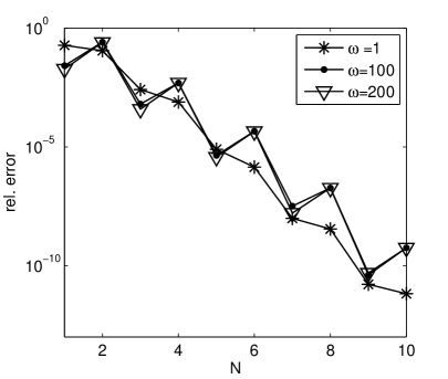
(a) Relative error of the approximation of $\int_{-1}^{1}\cos(x)\operatorname{e}^{i\omega x^{2}}$

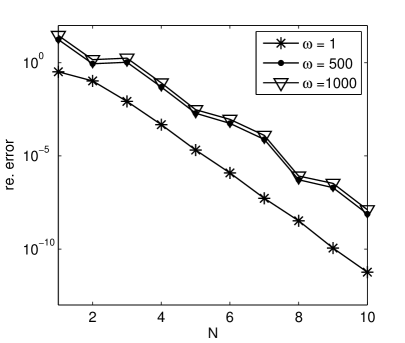
(b) Relative error of the approximation of $\int_{-1}^{1}\cos(x+1)\operatorname{e}^{i\omega\sin(x+1)}$

Figure 5.1: Quadrature error with respect to the polynomial degree $N$ for different integrals.

Table 1 and Table 2 show the effective ranks of the QTT approximations of $I_{\mathscr{R}}(\omega,T_{k})$ and $I_{\mathscr{I}}(\omega,T_{k})$ in various situations. It becomes evident that the choice of $g$ has only a minor influence on the corresponding QTT ranks. Even non-smooth functions, functions with stationary points and functions with unbounded first derivative are unproblematic. Another observation is that the influence of $k$ (degree of the Chebyshev polynomial) on the QTT ranks is very moderate even though the functions $I_{\mathscr{R}}(\omega,T_{k})$ and $I_{\mathscr{I}}(\omega,T_{k})$ become more oscillatory with increasing $k$. This is supported by the theory with states rank bounds that are independent of $k$.

$M$	$[\omega_{\min},\omega_{\max}]$	$\begin{matrix}g(x)=x,\\ k=2\end{matrix}$	$\begin{matrix}g(x)=x,\\ k=10\end{matrix}$	$\begin{matrix}g(x)=\frac{1}{2}x^{2}+\frac{1}{4}x,\\ k=2\end{matrix}$	$\begin{matrix}g(x)=\frac{1}{2}x^{2}+\frac{1}{4}x,\\ k=10\end{matrix}$
$2^{40}$	$[0,100]$	$4.6$	$4.9$	$4.5$	$4.7$
$2^{50}$	$[0,100]$	$4.2$	$4.4$	$4.2$	$4.2$
$2^{60}$	$[0,100]$	$3.8$	$4.1$	$3.8$	$3.9$
$2^{43}$	$[0,1000]$	$5.8$	$6.1$	$6.4$	$6.6$
$2^{53}$	$[0,1000]$	$5.2$	$5.5$	$5.8$	$6.0$
$2^{63}$	$[0,1000]$	$4.9$	$5.0$	$5.4$	$5.4$
$2^{43}$	$[0,2000]$	$6.2$	$6.5$	$7.2$	$7.4$
$2^{53}$	$[0,2000]$	$5.6$	$5.9$	$6.5$	$6.7$
$2^{63}$	$[0,2000]$	$5.2$	$5.4$	$6.0$	$6.1$

Table 1: Effective QTT-ranks of $M$-vectors related to the function $I_{\mathscr{R}}(\omega,T_{k})$ sampled on a uniform grid in the interval $[\omega_{\min},\omega_{\max}]$.

$M$	$[\omega_{\min},\omega_{\max}]$	$g(x)=\cos\left(x+\frac{1}{4}\right)$	$g(x)=\operatorname{e}^{x}$	$g(x)=\sin(x)^{2}\sqrt{x+1}$
$2^{42}$	$[0,500]$	$6.2$	7.2	6.0
$2^{52}$	$[0,500]$	$5.6$	6.5	5.5
$2^{62}$	$[0,500]$	$5.2$	6.0	5.0
$2^{42}$	$[500,700]$	$4.8$	5.1	4.5
$2^{52}$	$[500,700]$	$4.4$	4.6	4.0
$2^{62}$	$[500,700]$	$4.1$	4.3	3.7

Table 2: Effective QTT-ranks of $M$-vectors related to the function $I_{\mathscr{I}}(\omega,T_{5})$ sampled on a uniform grid in the interval $[\omega_{\min},\omega_{\max}]$.

If the approximation of $f$ is written in the form (3.4) then the functions $I_{\mathscr{R}}(\omega,L_{k})$ and $I_{\mathscr{I}}(\omega,L_{k})$, where $L_{k}$ is the $k$-th Lagrange basis polynomial, have to be precomputed. Table 3 shows the effective ranks of the QTT approximations of these functions. It can be seen that also in this case the ranks are low for different oscillators $g$, different $k$ and intervals $[\omega_{\min},\omega_{\max}]$. Using the Lagrange form of $f$ can be advantageous if $I(\omega,f)$ has to be approximated for many different functions $f$ since the Chebyshev coefficients do not have to be computed. On the other hand the form (3.2) can be favorable if the oscillator $g$ is an even or odd function since in this case the functions $I_{\mathscr{R}}(\omega,T_{k})$ and $I_{\mathscr{I}}(\omega,T_{k})$ are identical to zero for certain $k$ and therefore have neither to be precomputed nor evaluated (see Remark 3.4).

$M$	$[\omega_{\min},\omega_{\max}]$	$\begin{matrix}g(x)=x,\\ k=1\end{matrix}$	$\begin{matrix}g(x)=x,\\ k=5\end{matrix}$	$\begin{matrix}g(x)=\frac{1}{2}x^{2}+\frac{1}{4}x,\\ k=1\end{matrix}$	$\begin{matrix}g(x)=\frac{1}{2}x^{2}+\frac{1}{4}x,\\ k=5\end{matrix}$
$2^{43}$	$[0,1000]$	$6.1$	$5.8$	$6.6$	$6.4$
$2^{53}$	$[0,1000]$	$5.5$	$5.3$	$6.0$	$5.8$
$2^{63}$	$[0,1000]$	$5.0$	$4.9$	$5.5$	$5.3$

Table 3: Effective QTT-ranks of $M$-vectors related to the function $I_{\mathscr{R}}(\omega,L_{k})$ sampled on a uniform grid in the interval $[\omega_{\min},\omega_{\max}]$.

In Table 4 the computational time is illustrated that is needed to precompute $I_{\mathscr{R}}(\cdot,T_{k})$ via the QTT cross approximation algorithm. These timings mainly depend on the method that is used to compute $I_{\mathscr{R}}(\omega_{0},T_{k})$ at different points $\omega_{0}\in[\omega_{\min},\omega_{\max}]$ within this algorithm. As mentioned above we use a standard Gauss-Legendre quadrature rule to approximate these integrals. More precisely we divide the integration domain $[-1,1]$ into $\omega_{\max}$ subintervals and use $8$ quadrature points in each subinterval. Although this strategy has a suboptimal complexity, it is very general, easy to implement and leads to very accurate approximations of $I_{\mathscr{R}}(\omega_{0},T_{k})$. Since the cross approximation algorithm requires the computation of $I_{\mathscr{R}}(\omega_{0},T_{k})$ only at few grid points the computing times remain very moderate for different intervals, grid sizes and oscillators. Recall that in order to obtain approximations of $I_{\mathscr{R}}(\omega,f)$ the functions $I_{\mathscr{R}}(\omega,T_{k})$ have to be precomputed for $0\leq k\leq N$. Since these tasks are independent of each other, they can be easily performed in parallel.

$M$	$2^{43}$	$2^{53}$	$2^{63}$	$2^{43}$	$2^{53}$	$2^{63}$	$2^{43}$	$2^{53}$	$2^{63}$
$[\omega_{\min},\omega_{\max}]$	$[0,500]$			$[500,700]$			$[0,1000]$
$\begin{matrix}g(x)=x,\\ k=2\end{matrix}$	$12s$	$15s$	$17s$	$12s$	$17s$	$19s$	$20s$	$24s$	$25s$
$\begin{matrix}g(x)=\frac{1}{2}x^{2}+\frac{1}{4}x,\\ k=3\end{matrix}$	$12s$	$13s$	$15s$	$14s$	$17s$	$20s$	$19s$	$21s$	$25s$

Table 4: Computing times for the precomputation of $I_{\mathscr{R}}(\omega,T_{k})$ in seconds on an Intel Core i7-2600K processor.

Fourier integrals

Let $f:\mathbb{R}\rightarrow\mathbb{C}$ be an integrable function with $\operatorname{supp}f=[a,b]$. We are interested in computing the Fourier transform

$$\hat{f}(\omega) =\int_{a}^{b}f(x)\operatorname{e}^{-\operatorname{i}x\omega}dx$$ (5.1)

at different random points $\omega\in[\omega_{\min},\omega_{\max}]$. We define the affine scaling function $\chi_{a,b}(x):=\frac{b-a}{2}x+\frac{b+a}{2}$ and obtain

$$\hat{f}(\omega) =\frac{b-a}{2}\int_{-1}^{1}f\left(\chi_{a,b}(x)\right)\operatorname{e}^{-\operatorname{i}\cdot\chi_{a,b}(x)\cdot\omega}dx$$

$$=\frac{b-a}{2}\operatorname{e}^{-\operatorname{i}\cdot\frac{b+a}{2}\cdot\omega}\int_{-1}^{1}f\left(\chi_{a,b}(x)\right)\operatorname{e}^{-\operatorname{i}x\tilde{\omega}}dx.$$

with $\tilde{\omega}=\frac{b-a}{2}\omega$. The integration domain and the oscillator of the last integral are independent of $a$ and $b$. Thus, in order to approximate integrals of the form (5.1) for different intervals $[a,b]$, only the functions $I_{\mathscr{R}}(\cdot,T_{k})$ and $I_{\mathscr{I}}(\cdot,T_{k})$ with $g(x)=-x$ have to be precomputed in a sufficiently large interval. Note the ranks of the corresponding QTT tensors that can be observed numerically are very similar to the results in Table 3.

Exotic oscillators

Now, we consider oscillators which are not of the form $h_{\omega}(x)=\operatorname{e}^{\operatorname{i}\omega g(x)}$. Levin-type methods were introduced for the case of the Bessel oscillator $h_{\omega}(x)=J_{\nu}(\omega x)$ in [36], Filon-type methods were considered in [13] for oscillators of the form $h_{\omega}(x)=v(\sin(\omega\theta(x)))$. For most other types of oscillators such methods are not available so far. In Table 5 we show that our method can also be applied in these (and other) cases in the same way as before. Low ranks of the QTT approximations of the functions

$$I_{h_{\omega},k}(\omega):=\int_{-1}^{1}T_{k}(x)h_{\omega}(x)dx,\quad 1\leq k\leq N$$

can be observed in all tested cases.

$M$	$[\omega_{\min},\omega_{\max}]$	$\begin{matrix}h_{\omega}(x)=\\ J_{11}(\omega x)\end{matrix}$	$\begin{matrix}h_{\omega}(x)=\\ J_{8}^{2}(\omega x^{2})\end{matrix}$	$\begin{matrix}h_{\omega}(x)=\\ \cos(\sin(\omega x)+1)\end{matrix}$	$\begin{matrix}h_{\omega}(x)=\\ \Gamma(0.5\cdot\sin(\omega x)+2)\end{matrix}$
$2^{40}$	$[0,500]$	$5.4$	$5.7$	$7.2$	$7.3$
$2^{50}$	$[0,500]$	$4.9$	$5.2$	$6.5$	$6.5$
$2^{60}$	$[0,500]$	$4.5$	$4.7$	$6.0$	$5.9$

Table 5: Effective QTT-ranks of $M$-vectors related to the function $I_{h_{\omega},5}(\omega)$ sampled on a uniform grid in the interval $[\omega_{\min},\omega_{\max}]$.

5.2 Multi-dimensional integrals

In this paragraph we consider functions of the form

$$I_{\mathscr{R}}(\omega,L_{j_{1},\ldots,j_{d}})=\int_{[-1,1]^{d}}L_{j_{1}}(y_{1})\cdots L_{j_{d}}(y_{d})\cos(\omega g(y))dy$$ (5.2)

whose precomputation is necessary when (3.8) is used to approximate (3.7). Table 6 and 7 show the effective QTT ranks of the corresponding tensors for different oscillators $g$ in 2 and 3 dimensions. As before we can observe that the ranks are small in all tested situations. The computation of the integrals within the cross approximation scheme was performed using a tensorized version of the Gauss-Legendre quadrature described before.

$M$	$[\omega_{\min},\omega_{\max}]$	$\begin{matrix}g(x)=\\ x_{1}+x_{2}\end{matrix}$	$\begin{matrix}g(x)=\\ \sin(x_{1})/\sqrt{x_{1}x_{2}+3}\end{matrix}$
$2^{30}$	$[0,100]$	$5.2$	$4.4$
$2^{40}$	$[0,100]$	$4.6$	$3.9$
$2^{50}$	$[0,100]$	$4.2$	$3.5$

Table 6: Effective QTT-ranks of $M$-vectors related to the function $I_{\mathscr{R}}(\omega,L_{2,5})$ for $d=2$ sampled on a uniform grid in the interval $[\omega_{\min},\omega_{\max}]$.

$M$	$[\omega_{\min},\omega_{\max}]$	$\begin{matrix}g(x)=\\ x_{1}+x_{2}+x_{3}\end{matrix}$	$\begin{matrix}g(x)=\\ \sin(x_{1}x_{3})/\sqrt{x_{1}x_{2}+3}\end{matrix}$
$2^{30}$	$[0,50]$	$6.1$	$4.3$
$2^{40}$	$[0,50]$	$5.5$	$3.9$
$2^{50}$	$[0,50]$	$5.3$	$3.7$

Table 7: Effective QTT-ranks of $M$-vectors related to the function $I_{\mathscr{R}}(\omega,L_{2,5,3})$ for $d=3$ sampled on a uniform grid in the interval $[\omega_{\min},\omega_{\max}]$.

6 Conclusion

We described a new approach for the efficient approximation of highly oscillatory weighted integrals. The main idea of our approach is to compute a priory and then represent in low-parametric tensor formats certain $\omega$-dependent prototype functions (which by itself consist of oscillatory integrals), whose evaluation lead in a straightforward way to approximations of the target integral. The QTT approximation method for long functional $m$-vectors allows the accurate approximation and efficient $\log m$-storage of these functions in the wide range of grid and frequency parameters. Numerical examples illustrate the efficiency of the QTT-based numerical integration scheme on many nontrivial examples in one and several spatial dimensions. This demonstrates the promising features of the method for further applications to the general class of highly oscillating integrals and for the solution of ODEs and PDEs with oscillating or/and quasi-periodic coefficients arising in computational physics and chemistry as well as in homogenization techniques.

Acknowledgement. A large part of this research was conducted during a stay of the second author at the Max Planck Institute for Mathematics in the Sciences in Leipzig. The financial support is greatly acknowledged.

References

- [1] A. Asheim, A. Deano, D. Huybrechs, and H. Wang. A Gaussian quadrature rule for oscillatory integrals on a bounded interval. Discrete and Continuous Dynamical Systems, 34(3):883–901, 2014.
- [2] A. Deano and D. Huybrechs. Complex Gaussian quadrature of oscillatory integrals. Numerische Mathematik, 112(2):197–219, 2009.
- [3] S. V. Dolgov. Tensor product methods in numerical simulation of high-dimensional dynamical problems. PhD thesis, University of Leipzig, 2014.
- [4] V. Dom nguez, I. Graham, and T. Kim. Filon–Clenshaw–Curtis rules for Highly Oscillatory Integrals with Algebraic Singularities and Stationary Points. SIAM Journal on Numerical Analysis, 51(3):1542–1566, 2013.
- [5] V. Dom nguez, I. G. Graham, and V. P. Smyshlyaev. Stability and error estimates for Filon–Clenshaw–Curtis rules for highly oscillatory integrals. IMA Journal of Numerical Analysis, 31(4):1253–1280, 2011.
- [6] L. Grasedyck. Polynomial approximation in hierarchical Tucker format by vector-tensorization. DFG-SPP1324 Preprint 43, Philipps-Univ., Marburg, 2010.
- [7] L. Grasedyck, D. Kressner, and C. Tobler. A literature survey of low-rank tensor approximation techniques. arXiv preprint 1302.7121, 2013.
- [8] W. Hackbusch. Tensor spaces and numerical tensor calculus. Springer–Verlag, Berlin, 2012.
- [9] M. Hochbruck and C. Lubich. On Magnus integrators for time-dependent Schrödinger equations. SIAM J. Numer. Anal., 41(3):945–963, 2003.
- [10] D. Huybrechs and S. Olver. Highly Oscillatory Problems, chapter 2: Highly Oscillatory Quadrature, pages 25–50. Cambridge University Press, 2009.
- [11] D. Huybrechs and S. Vandewalle. On the evaluation of highly oscillatory integrals by analytic continuation. SIAM J. Numer. Anal., 44(3):1026–1048, 2006.
- [12] A. Iserles. On the global error of discretization methods for highly-oscillatory ordinary differential equations. BIT, 42:561–599, 2002.
- [13] A. Iserles and D. Levin. Asymptotic expansion and quadrature of composite highly oscillatory integrals. Math. Comp., 80:279–296, 2011.
- [14] A. Iserles and S. Nørsett. Efficient quadrature of highly oscillatory integrals using derivatives. Proceedings of the Royal Society A: Mathematical, Physical and Engineering Science, 461(2057):1383–1399, 2005.
- [15] A. Iserles and S. Nørsett. From high oscillation to rapid approximation I: Modified Fourier expansions. IMA J. Num. Anal, 28:862–887, 2008.
- [16] A. Iserles, S. Nørsett, and S. Olver. Highly oscillatory quadrature: The story so far. In A. de Castro, D. G mez, P. Quintela, and P. Salgado, editors, Numerical Mathematics and Advanced Applications, pages 97–118. Springer Berlin Heidelberg, 2006.
- [17] V. Khoromskaia and B. N. Khoromskij. Grid-based lattice summation of electrostatic potentials by assembled rank-structured tensor approximation. Comp. Phys. Communications, 185(1):3162–3174, 2014.
- [18] V. Khoromskaia and B. N. Khoromskij. Tensor approach to linearized Hartree-Fock equation for lattice-type and periodic systems. MPI MIS preprint 62, 2014.
- [19] B. Khoromskij, S. Sauter, and A. Veit. Fast Quadrature Techniques for Retarded Potentials Based on TT/QTT Tensor Approximation. Computational Methods in Applied Mathematics, 11(3):342–362, 2011.
- [20] B. N. Khoromskij. -Quantics approximation of -d tensors in high-dimensional numerical modeling. Preprint 55, MPI MIS, Leipzig, 2009.
- [21] B. N. Khoromskij. –Quantics approximation of – tensors in high-dimensional numerical modeling. Constr. Appr., 34(2):257–280, 2011.
- [22] B. N. Khoromskij. Tensor-structured numerical methods in scientific computing: survey on recent advances. Chemometr. Intell. Lab. Syst., 110(1):1–19, 2012.
- [23] B. N. Khoromskij. Tensor Numerical Methods for Multidimensional PDEs: Basic Theory and Initial Applications. ESAIM: Proceedings and Surveys, N. Champagnat, T. Leliévre, A. Nouy, eds, 48:1–28, December 2014.
- [24] T. Kolda and B. Bader. Tensor decompositions and applications. SIAM Review, 51/3:455–500, 2009.
- [25] S. Olver. Moment-free numerical integration of highly oscillatory functions. IMA Journal of Numerical Analysis, 26(2):213–227, 2006.
- [26] S. Olver. Numerical Approximation of Highly Oscillatory Integrals. PhD thesis, University of Cambridge, 2008.
- [27] I. Oseledets and E. Tyrtyshnikov. TT-cross approximation for multidimensional arrays. Linear Algebra and its Applications, 432(1):70 – 88, 2010.
- [28] I. V. Oseledets. Approximation of matrices using tensor decomposition. SIAM J. Matrix Anal. Appl., 31(4):2130–2145, 2010.
- [29] I. V. Oseledets. Constructive representation of functions in low-rank tensor formats. Constr. Appr., 37(1):1–18, 2013.
- [30] I. V. Oseledets and E. E. Tyrtyshnikov. Breaking the curse of dimensionality, or how to use SVD in many dimensions. SIAM J. Sci. Comput., 31(5):3744–3759, 2009.
- [31] L. Trefethen. Is Gauss Quadrature Better than Clenshaw-Curtis? SIAM Rev., 50:67–87, February 2008.
- [32] L. N. Trefethen. Approximation theory and approximation practice. Siam, 2013.
- [33] F. Verstraete, D. Porras, and J. I. Cirac. Density matrix renormalization group and periodic boundary conditions: A quantum information perspective. Phys. Rev. Lett., 93(22):227205, 2004.
- [34] G. Vidal. Efficient classical simulation of slightly entangled quantum computations. Phys. Rev. Lett., 91(14), 2003.
- [35] S. R. White. Density-matrix algorithms for quantum renormalization groups. Phys. Rev. B, 48(14):10345–10356, 1993.
- [36] S. Xiang, W. Gui, and P. Mo. Numerical quadrature for Bessel transformations. Applied Numerical Mathematics, 58(9):1247 – 1261, 2008.
- [37] S. Xiang, G. He, and Y. Cho. On error bounds of Filon-Clenshaw-Curtis quadrature for highly oscillatory integrals. Advances in Computational Mathematics, pages 1–25, 2014.