Fully Adaptive Newton-Galerkin Methods for Semilinear Elliptic Partial Differential Equations

Abstract.

In this paper we develop an adaptive procedure for the numerical solution of general, semilinear elliptic problems with possible singular perturbations. Our approach combines both a prediction-type adaptive Newton method and an adaptive finite element discretization (based on a robust a posteriori error analysis), thereby leading to a fully adaptive Newton-Galerkin scheme. Numerical experiments underline the robustness and reliability of the proposed approach for different examples.

1. Introduction

The focus of this paper is the numerical approximation of semilinear elliptic problems with possible singular perturbations. More precisely, for a fixed parameter $\varepsilon>0$ (possibly with $\varepsilon\ll 1$), and a continuously differentiable function $f:\,\mathbb{R}\to\mathbb{R}$, we consider the problem of finding a function $u:\,\Omega\to\mathbb{R}$ which satisfies

$$-\varepsilon\Delta u =f(u)\text{ in }\ \Omega,\qquad u=0\text{ on }\partial\Omega.$$ (1)

Here, $\Omega\subset\mathbb{R}^{d}$, with $d=1$ or $d=2$, is an open and bounded 1d interval or a 2d Lipschitz polygon, respectively. Problems of this type appear in a wide range of applications including, e.g., nonlinear reaction-diffusion in ecology and chemical models [5, 9, 12, 16, 17], economy [3], or classical and quantum physics [4, 24].

From an analysis point of view, semilinear elliptic boundary value problems (1) have been studied in detail by a number of authors over the last decades; we refer, e.g., to the monographs [1, 19, 23] and the references therein. In particular, solutions of (1) are known to be typically not unique (even infinitely many solutions may exist), and, in the singularly perturbed case, to exhibit boundary layers, interior shocks, and (multiple) spikes. The existence of multiple solutions due to the nonlinearity of the problem and/or the appearance of singular effects constitute two challenging issues when solving problems of this type numerically; see, e.g.,[20, 27].

Nowadays the use of the Newton-Raphson method in dealing with nonlinear phenomena is standard. Indeed, this method is highly successful if initial guesses are chosen close enough to a solution and if the basins of attraction for different solutions are sufficiently well-behaved for the Newton iteration to stay within the same attractor. As a consequence, on a local level, the scheme is often celebrated for its quadratic convergence regime close to a root. From a global perspective, however, the Newton method is well-known to exhibit chaotic behavior. Indeed, applying the Newton method to algebraic systems of equations, for example, may result in highly complex or even fractal attractor boundaries of the associated roots; see, e.g., [18]. This is related to the fact that the Newton iteration may be unstable in the sense that, farther away from a root, iterates may switch from one basin of attraction to another, and hence, converge to an undesired root (or even diverge). In the context of semilinear elliptic PDE the situation is even worse (and yet more severe in the singularly perturbed case): In fact, for certain types of problems, the Newton iteration will typically tend to become unbounded, and hence, will not approach a sensible solution at all; see, e.g., [6], where this issue has been addressed for a certain class of problems by means of a suitable rescaling technique in each step. A frequently employed remedy to tame (although not to eliminate) the chaotic behavior of Newton’s method is the use of damping to avoid the appearance of possibly large updates in the iterations. An even more sophisticated way to further improve the quality of the results is the application of variable damping; see, e.g., the extensive overview [7] or [8, 10] for different variations of the classical Newton scheme. The idea of adaptively adjusting the magnitude of the Newton updates has also been studied in the recent articles [2, 21]; there, following, e.g., [15, 18, 22], the Newton method was identified as the numerical discretization of a specific ordinary differential equation (ODE)—the so-called continuous Newton method—by the explicit Euler scheme, with a fixed step size $k=1$. Then, in order to tame the chaotic behavior of the Newton iterations, the idea presented in [2, 21] is based on discretizing the continuous Newton ODE by the explicit Euler method with variable step sizes, and to combine it with a simple step size control procedure; in particular, the resulting algorithm retains the optimal step size $k=1$ whenever sensible and is able to deal with singularities in the iterations more carefully than the classical Newton scheme. In fact, numerical experiments for algebraic and differential equations in [2, 21] revealed that the new method is able to generate attractors with almost smooth boundaries, whereas the traditional Newton method produces fractal Julia sets; moreover, the numerical tests demonstrated an improved convergence rate not matched on average by the classical Newton method.

In the present paper, our goal is to extend the approach developed in [2, 21] to the numerical solution of (1). To this end, we will start by applying an adaptive Newton scheme, which is based on some simple prediction strategies, to the nonlinear boundary value problem (1). Subsequently, we discretize the resulting sequence of linear problems by a standard $\mathbb{P}_{1}$-finite element method (FEM); note that this approach is in contrast to solving the nonlinear algebraic system resulting from a FEM discretization of the original PDE with the aid of the Newton method (see, e.g., the work on inexact Newton methods [11]). In order to control the approximation error caused by the FEM discretization, we derive a residual-based a posteriori error analysis which allows to adaptively refine the finite element mesh; here, following the approach in [25], we will take particular care of the singular perturbation in order to obtain $\varepsilon$-robust error estimates. The final error estimate (Theorem 4.4) bounds the error in terms of the (elementwise) finite element approximation (FEM-error) and the error caused by the linearization of the original problem due to Newton’s method (Newton-error). Then, in order to define a fully adaptive Newton-Galerkin scheme, we propose an interplay between the adaptive Newton-Raphson method and the adaptive finite element approach: More precisely, as the adaptive procedure is running, we either perform a Newton-Raphson step in accordance with our prediction strategy (Section 2) or refine the current mesh based on the a posteriori error analysis (Section 4), depending on which error (FEM-error or Newton-error) is more dominant in the current iteration step. Our numerical results will reveal that sensible solutions can be found even in the singularly perturbed case, and that our scheme is reliable for reasonable choices of initial guesses, and $\varepsilon$-robust.

For the purpose of this paper, we suppose that a (not necessarily unique) solution $u\in X:=H^{1}_{0}(\Omega)$ of (1) exists; here, we denote by $H^{1}_{0}(\Omega)$ the standard Sobolev space of functions in $H^{1}(\Omega)=W^{1,2}(\Omega)$ with zero trace on $\partial\Omega$. Furthermore, signifying by $X^{\prime}=H^{-1}(\Omega)$ the dual space of $X$, and upon defining the map $\mathsf{F}_{\varepsilon}:X\rightarrow X^{\prime}$ through

$$\left\langle\mathsf{F}_{\varepsilon}(u),v\right\rangle:=\int_{\Omega}\left\{\varepsilon\nabla u\cdot\nabla v-f(u)v\right\}\,\mathsf{d}\bm{x}\qquad\forall v\in X,$$ (2)

where $\left\langle\cdot,\cdot\right\rangle$ is the dual product in $X^{\prime}\times X$, the above problem (1) can be written as a nonlinear operator equation in $X^{\prime}$:

$$u\in X:\qquad\mathsf{F}_{\varepsilon}(u)=0.$$ (3)

In addition, on any subset $D\subseteq\Omega$, we introduce the norm

$$\left|\!\left|\!\left|u\right|\!\right|\!\right|_{\varepsilon,D}:=\Bigl{(}\varepsilon\left\|\nabla u\right\|_{0,D}^{2}+\left\|u\right\|_{0,D}^{2}\Bigr{)}^{\nicefrac{{1}}{{2}}},$$ (4)

where $\|\cdot\|_{0,D}$ denotes the $L^{2}$-norm on $D$. Note that, in the case of $f(u)=-u$, when (1) is linear and strongly elliptic, the norm $\left|\!\left|\!\left|\cdot\right|\!\right|\!\right|_{\varepsilon,\Omega}$ is a natural energy norm on $X$. Frequently, for $D=\Omega$, the subindex ‘$D$’ will be omitted. Furthermore, the associated dual norm of $\mathsf{F}_{\varepsilon}$ from (2) is given by

$$\left|\!\left|\!\left|\mathsf{F}_{\varepsilon}(u)\right|\!\right|\!\right|_{X^{\prime},\varepsilon}=\sup_{\genfrac{}{}{0.0pt}{}{v\in X}{\left|\!\left|\!\left|v\right|\!\right|\!\right|_{\varepsilon}=1}}\int_{\Omega}\left\{\varepsilon\nabla u\cdot\nabla v-f(u)v\right\}\,\mathsf{d}\bm{x}.$$

Throughout this work we shall use the abbreviation $x\preccurlyeq y$ to mean $x\leq cy$, for a constant $c>0$ independent of the mesh size $h$ and of $\varepsilon>0$.

The paper is organized as follows: In Section 2 we will consider the Newton-Raphson method within the context of dynamical systems in general Banach spaces, and present two prediction strategies for controlling the Newton step size parameter. Furthermore, Section 3 focuses on the application of the Newton-Raphson method to semilinear elliptic problems. In addition, we discuss the discretization of the problems under consideration by finite element methods in Section 4, and derive an $\varepsilon$-robust a posteriori error analysis. A series of numerical experiments illustrating the performance of the fully adaptive Newton-Galerkin scheme proposed in this work will be presented as well. Finally, we summarize our findings in Section 5.

2. Adaptive Newton-Raphson Methods in Banach Spaces

In the following section we shall briefly revisit the adaptive Newton algorithm from [2], and additionally, will derive an improved variant of our previous work.

2.1. Abstract Framework

Let $X,Y$ be two Banach spaces, with norms $\|\cdot\|_{X}$ and $\|\cdot\|_{Y}$, respectively. Given an open subset $\Xi\subset X$, and a (possibly nonlinear) operator $\mathsf{F}:\,\Xi\to Y$, we consider the nonlinear operator equation

$$\mathsf{F}(u)=0,$$ (5)

for some unknown zeros $u\in\Xi$. Supposing that the Fréchet derivative $\mathsf{F}^{\prime}$ of $\mathsf{F}$ exists in $\Xi$ (or in a suitable subset), the classical Newton-Raphson method for solving (5) starts from an initial guess $u_{0}\in\Xi$, and generates the iterates

$$u_{n+1}=u_{n}+\delta_{n},\qquad n\geq 0,$$ (6)

where the update $\delta_{n}\in X$ is implicitly given by the linear equation

$$\mathsf{F}^{\prime}(u_{n})\delta_{n}=-\mathsf{F}(u_{n}),\qquad n\geq 0.$$

Naturally, for this iteration to be well-defined, we need to assume that $\mathsf{F}^{\prime}(u_{n})$ is invertible for all $n\geq 0$, and that $\{u_{n}\}_{n\geq 0}\subset\Xi$.

2.2. A Simple Prediction Strategy

In order to improve the reliability of the Newton method (6) in the case that the initial guess $u_{0}$ is relatively far away from a root $u_{\infty}\in\Xi$ of $\mathsf{F}$, $\mathsf{F}(u_{\infty})=0$, introducing some damping in the Newton-Raphson method is a well-known remedy. In that case (6) is rewritten as

$$u_{n+1}=u_{n}-k_{n}\mathsf{F}^{\prime}(u_{n})^{-1}\mathsf{F}(u_{n}),\qquad n\geq 0,$$ (7)

where $k_{n}>0$, $n\geq 0$, is a damping parameter that may be adjusted adaptively in each iteration step.

Provided that $\mathsf{F}^{\prime}(u)$ is invertible on a suitable subset of $\Xi\subset X$, we define the Newton-Raphson Transform by

$$u\mapsto\mathsf{N}_{\mathsf{F}}(u):=-\mathsf{F}^{\prime}(u)^{-1}\mathsf{F}(u).$$

Then, rearranging terms in (7), we notice that

$$\frac{u_{n+1}-u_{n}}{k_{n}}=\mathsf{N}_{\mathsf{F}}(u_{n}),\qquad n\geq 0,$$ (8)

i.e., (7) can be seen as the discretization of the Davydenko-type system,

$$\begin{split}\dot{u}(t)&=\mathsf{N}_{\mathsf{F}}(u(t)),\quad t\geq 0,\qquad u(0)=u_{0},\end{split}$$ (9)

by the forward Euler scheme with step size $k_{n}>0$.

For $t\in[0,\infty)$, the solution $u(t)$ of (9) defines a trajectory in $X$ that begins at $u_{0}$, and that will potentially converge to a zero of $\mathsf{F}$ as $t\to\infty$. Indeed, this can be seen (formally) from the integral form of (9), that is,

$$\mathsf{F}(u(t))=\mathsf{F}(u_{0})e^{-t},\qquad t\geq 0,$$ (10)

which implies that $\mathsf{F}(u(t))\to 0$ as $t\to\infty$.

Now taking the view of dynamical systems, our goal is to compute an upper bound for the value of the step sizes $k_{n}>0$ from (7), $n\geq 0$, so that the discrete forward Euler solution $\{u_{n}\}_{n\geq 0}$ from (7) stays reasonably close to the continuous solution of (9). To this end, we approximate the trajectory $u$ from (9) close to the initial value $u_{0}$ by a second-order Taylor expansion:

$$u(t)\approx u_{0}+t\dot{u}(0)+t^{2}\xi,$$ (11)

for some (fixed) $\xi\in X$ to be determined. Using the integral form (10), we see that

$$\mathsf{F}(u_{0})e^{-t}=\mathsf{F}(u(t))\approx\mathsf{F}(u_{0}+t\dot{u}(0)+t^{2}\xi),$$

where a Taylor expansion of $\mathsf{F}$ leads to $\mathsf{F}(u_{0})e^{-t}\approx\mathsf{F}(u_{0})+\mathsf{F}^{\prime}(u_{0})(t\dot{u}(0)+t^{2}\xi)$. Moreover, from (9) we observe that

$$\dot{u}(0)=\mathsf{N}_{\mathsf{F}}(u_{0}),$$ (12)

or equivalently, $\mathsf{F}^{\prime}(u_{0})\dot{u}(0)=-\mathsf{F}(u_{0})$, and hence $\mathsf{F}(u_{0})(e^{-t}+t-1)\approx t^{2}\mathsf{F}^{\prime}(u_{0})\xi$. Approximating $e^{-t}\approx 1-t+\frac{1}{2}t^{2}$ results in

$$\xi\approx\frac{1}{2}\mathsf{F}^{\prime}(u_{0})^{-1}\mathsf{F}(u_{0})=-\frac{1}{2}\mathsf{N}_{\mathsf{F}}(u_{0}).$$ (13)

Combining (11) and (13) yields

$$\|u(k_{0})-u_{1}\|_{X}\approx k_{0}^{2}\|\xi\|_{X}\approx\frac{k_{0}^{2}}{2}\|\mathsf{N}_{\mathsf{F}}(u_{0})\|_{X},$$

where $u_{1}=u_{0}+k_{0}\mathsf{N}_{\mathsf{F}}(u_{0})$ is the first Newton iterate from (7) (with $n=0$). Recalling that $u_{1}$ may also be seen as the forward Euler approximation (with step size $k_{0}>0$) of the solution $u$ of (9) at $t=k_{0}$, the above relation can be understood as the nodal error between the solution of (9) and its numerical approximation after the first time step. Then, for a given error tolerance $\tau>0$, choosing

$$k_{0}=\sqrt{\frac{2\tau}{\|\mathsf{N}_{\mathsf{F}}(u_{0})\|_{X}}},$$

we arrive at $\|u(k_{0})-u_{1}\|_{X}\approx\tau$, i.e., the exact trajectory given by the solution of (9) and its forward Euler approximation from (7) remain $\tau$-close in the $\|.\|_{X}$-norm for the given time step $k_{0}$.

Iterating the above observations leads to the following prediction strategy for the selection of $k_{n}$ in (7). Incidentally, the resulting algorithm is identical with the one presented in [2, Algorithm 2.1] although our derivation here is different.

Algorithm 2.1.

Fix a tolerance $\tau>0$.

1. Start the Newton iteration with an initial guess $u_{0}\in\Xi$.

2. In each iteration step $n=0,1,2,\ldots$, compute

   $$k_{n}=\min\left(\sqrt{\frac{2\tau}{\left\|\mathsf{N}_{\mathsf{F}}(u_{n})\right\|_{X}}},1\right).$$ (14)

3. Compute $u_{n+1}$ based on the Newton iteration (7), and go to (ii) with $n\leftarrow n+1$.

Remark 2.2.

The minimum in (14) ensures that the step size $k_{n}$ is chosen to be 1 whenever possible. Indeed, this is required in order to guarantee quadratic convergence of the Newton iteration close to a root (provided that the root is simple).

Remark 2.3.

Under certain conditions it can been proved that the above algorithm does in fact converge to a zero of $\mathsf{F}$; see [2, Theorem 2.4].

2.3. An Improved Prediction Strategy

In Section 2.2 our step size prediction strategy is based on approximating the solution of the Davydenko-type system (9) by the use of (11). We can improve this approach by looking at the Taylor expansion

$$u(t)=u_{0}+t\dot{u}(0)+\frac{1}{2}t^{2}\ddot{u}(0)+\mathcal{O}(t^{3})$$ (15)

of the trajectory $u$ defined by (9). Recalling (12) we can replace $\dot{u}(0)$ above by the Newton-Raphson transform $\mathsf{N}_{\mathsf{F}}(u_{0})$, however, we still need to find a good approximation of $\ddot{u}(0)$. This can be accomplished by taking the derivative of (9) with respect to $t$ at $t=0$. Applying the chain rule gives

$$\ddot{u}(0)=\mathsf{N}_{\mathsf{F}}^{\prime}(u_{0})\dot{u}(0)=\mathsf{N}_{\mathsf{F}}^{\prime}(u_{0})\mathsf{N}_{\mathsf{F}}(u_{0}).$$

Since it is preferable to avoid the explicit appearance of $\mathsf{N}_{\mathsf{F}}^{\prime}(u_{0})$ we look at, for some small $h>0$, the Taylor expansion

$$\mathsf{N}_{\mathsf{F}}(u_{0}+h\mathsf{N}_{\mathsf{F}}(u_{0}))=\mathsf{N}_{\mathsf{F}}(u_{0})+h\mathsf{N}_{\mathsf{F}}^{\prime}(u_{0})\mathsf{N}_{\mathsf{F}}(u_{0})+\mathcal{O}(h^{2}\|\mathsf{N}_{\mathsf{F}}(u_{0})\|_{X}^{2}).$$

We conclude

$$\ddot{u}(0)=\mathsf{N}_{\mathsf{F}}^{\prime}(u_{0})\mathsf{N}_{\mathsf{F}}(u_{0})=\frac{1}{h}\eta_{h}+\mathcal{O}(h\|\mathsf{N}_{\mathsf{F}}(u_{0})\|_{X}^{2}),$$

with $\eta_{h}=\mathsf{N}_{\mathsf{F}}(u_{0}+h\mathsf{N}_{\mathsf{F}}(u_{0}))-\mathsf{N}_{\mathsf{F}}(u_{0})$. Inserting this identity into (15) and employing (12), we arrive at

$$u(t)=u_{0}+t\mathsf{N}_{\mathsf{F}}(u_{0})+\frac{t^{2}}{2h}\eta_{h}+\mathcal{O}(t^{3})+\mathcal{O}(t^{2}h\|\mathsf{N}_{\mathsf{F}}(u_{0})\|_{X}^{2}).$$

Hence, after the first time step of length $k_{0}>0$ there holds

$$u(k_{0})-u_{1}=\frac{k_{0}^{2}}{2h}\eta_{h}+\mathcal{O}(k_{0}^{3})+\mathcal{O}(k_{0}^{2}h\|\mathsf{N}_{\mathsf{F}}(u_{0})\|_{X}^{2}),$$ (16)

where $u_{1}$ is the forward Euler solution from (7). Then, for a prescribed tolerance $\tau>0$ as before, we have $\|u(k_{0})-u_{1}\|_{X}\approx\tau$ if we set $k_{0}=\sqrt{2\tau h\|\eta_{h}\|_{X}^{-1}}$. In order to balance the $\mathcal{O}$-terms in (16) it is reasonable to make the choice $h=\mathcal{O}(k_{0}\|\mathsf{N}_{\mathsf{F}}(u_{0})\|_{X}^{-2})$, i.e.,

$$h=\gamma k_{0}\|\mathsf{N}_{\mathsf{F}}(u_{0})\|_{X}^{-2},$$ (17)

for some parameter $\gamma>0$.

With these calculations we can improve the previous Algorithm 2.1 as follows:

Algorithm 2.4.

Fix a tolerance $\tau>0$ and a parameter $\gamma>0$, and set $n=0$.

1. Start the Newton iteration with an initial guess $u_{0}\in\Xi$.

2. If $n=0$, then choose

   $$\kappa_{0}=\min\left(\sqrt{\frac{2\tau}{\left\|\mathsf{N}_{\mathsf{F}}(u_{0})\right\|_{X}}},1\right),$$

   according to Algorithm 2.1, else if $n\geq 1$, let $\kappa_{n}=k_{n-1}$. Moreover, set $h_{n}=\gamma\kappa_{n}\|\mathsf{N}_{\mathsf{F}}(u_{n})\|_{X}^{-2}$ based on (17), and define

   $$k_{n}=\min\left(\sqrt{\frac{2\tau h_{n}}{\left\|\mathsf{N}_{\mathsf{F}}(u_{0}+h_{n}\mathsf{N}_{\mathsf{F}}(u_{0}))-\mathsf{N}_{\mathsf{F}}(u_{0})\right\|_{X}}},1\right).$$ (18)

3. Compute $u_{n+1}$ based on the Newton iteration (7), and go to (ii) with $n\leftarrow n+1$.

Remark 2.5.

In contrast to the simple prediction strategy from Section 2.2, Algorithm 2.4 is based on the improved Taylor approximation (15). This will naturally lead to more reliable results in the adaptive Newton iteration, since the discrete system (8) will supposedly follow the continuous dynamics of (9) more closely. Evidently, the price to pay is one additional evaluation of the Newton-Raphson transform in each time step of the discrete dynamical system (7); cf. (18). This will roughly increase the complexity of Algorithm 2.1 by a constant factor of 2.

Remark 2.6.

The preset tolerance $\tau$ in the above adaptive strategies will typically be fixed a priori. Here, for highly nonlinear problems featuring numerous or even infinitely many solutions, it is recommendable to select $\tau\ll 1$ small in order to increase the chances of remaining within the attractor of the given initial guess. This is particularly important if the starting value is relatively far away from a solution.

3. Application to Semilinear Elliptic Problems

In order to apply an adaptive Newton-Raphson method as introduced in Section 2 to the nonlinear PDE problem (3), note that the Fréchet-derivative of $\mathsf{F}_{\varepsilon}$ from (3) at $u\in X$ is given, by

$$\left\langle\mathsf{F}_{\varepsilon}^{\prime}(u)w,v\right\rangle=\int_{\Omega}\left\{\varepsilon\nabla w\cdot\nabla v-f^{\prime}(u)wv\right\}\,\mathsf{d}\bm{x},\qquad v,w\in X=H^{1}_{0}(\Omega).$$

We note that, if there is a constant $\beta>0$ for which $f^{\prime}(u)\in L^{1+\beta(d-1)}(\Omega)$, then $\mathsf{F}_{\varepsilon}^{\prime}(u)$ is a well-defined linear mapping from $X$ to $X^{\prime}$; see Lemma A.1.

Then, given an initial guess $u_{0}\in X$ for (3), the Newton method (7) is to find $u_{n+1}\in X$ from $u_{n}\in X$, $n\geq 0$, such that

$$\mathsf{F}_{\varepsilon}^{\prime}(u_{n})(u_{n+1}-u_{n})=-k_{n}\mathsf{F}_{\varepsilon}(u_{n}),$$

in $X^{\prime}$. Equivalently,

$$a_{\varepsilon}(u_{n};u_{n+1},v)=a_{\varepsilon}(u_{n};u_{n},v)-k_{n}\ell_{\varepsilon}(u_{n};v)\qquad\forall v\in X,$$ (19)

where, for fixed $u\in X$,

$$a_{\varepsilon}(u;w,v) :=\int_{\Omega}\left\{\varepsilon\nabla w\cdot\nabla v-f^{\prime}(u)wv\right\}\,\mathsf{d}\bm{x},$$

$$l_{\varepsilon}(u;v) :=\int_{\Omega}\left\{\varepsilon\nabla u\cdot\nabla v-f(u)v\right\}\,\mathsf{d}\bm{x}$$

are bilinear and linear forms on $X\times X$ and $X$, respectively.

Remark 3.1.

Let us consider a special case, where the weak formulation (19), for given $u_{n}$, always has a (unique) solution $u_{n+1}\in X$. To this end, we assume that there are constants $\underline{\lambda},\overline{\lambda}\geq 0$ with $\varepsilon C_{P}^{-2}>\overline{\lambda}$ such that $-\underline{\lambda}\leq f^{\prime}(u)\leq\overline{\lambda}$ holds for all $u\in\mathbb{R}$. Here, $C_{P}=C_{P}(\Omega)>0$ is the constant in the Poincaré inequality on $\Omega$:

$$\|w\|_{0}\leq C_{P}\|\nabla w\|_{0}\qquad\forall w\in X.$$ (20)

Then, for any given $u_{n}\in X$ the linear problem (19) has a unique solution $u_{n+1}\in X$.

Proof.

Our goal is to apply the Lax-Milgram Lemma. For this purpose, we will show that $a_{\varepsilon}(u_{n};\cdot,\cdot)$ is a bounded and coercive bilinear form on $X\times X$, and that $l_{\varepsilon}(u_{n};\cdot)$ is a bounded linear form on $X$.

By definition of the bilinear form $a_{\varepsilon}(u_{n};\cdot,\cdot)$ we have

$$a(u_{n};w,w) =\int_{\Omega}\{\varepsilon|\nabla w|^{2}-f^{\prime}(u_{n})w^{2}\}\,\mathsf{d}\bm{x}$$

$$=\varepsilon\int_{\Omega}{|\nabla w|^{2}}\,\mathsf{d}\bm{x}-\int_{M_{f}^{\complement}}{f^{\prime}(u_{n})w^{2}}\,\mathsf{d}\bm{x}-\int_{M_{f}}{f^{\prime}(u_{n})w^{2}}\,\mathsf{d}\bm{x}.$$

Here, $M_{f}=\{\bm{x}\in\Omega:\,(f^{\prime}\circ u_{n})(\bm{x})>0\}$. Then,

$$a(u_{n};w,w)\geq\varepsilon\int_{\Omega}{|\nabla w|^{2}}\,\mathsf{d}\bm{x}-\overline{\lambda}\int_{M_{f}}{w^{2}}\,\mathsf{d}\bm{x}\geq\varepsilon\int_{\Omega}{|\nabla w|^{2}}\,\mathsf{d}\bm{x}-\overline{\lambda}\int_{\Omega}{w^{2}}\,\mathsf{d}\bm{x}.$$ (21)

Invoking the Poincaré inequality (21) results in $a(u_{n};w,w)\geq(\varepsilon-\overline{\lambda}C_{p}^{2})\left\|\nabla w\right\|_{0,\Omega}^{2}$, which, by the equivalence of the $H^{1}$-seminorm and the norm $\left|\!\left|\!\left|\cdot\right|\!\right|\!\right|_{\varepsilon}$ from (4) on $X$ (resulting from the Poincaré inequality (20)), shows that $a(u_{n};\cdot,\cdot)$ is coercive by assumption on the difference $\varepsilon-\overline{\lambda}C_{p}^{2}>0$.

Furthermore, $a(u_{n};\cdot,\cdot)$ is bounded. Indeed, for $v,w\in X$ there holds

$$|a(u_{n};v,w)| \leq\varepsilon\int_{\Omega}|\nabla w||\nabla v|\,\mathsf{d}\bm{x}+\sup_{x\in\mathbb{R}}|f^{\prime}(x)|\int_{\Omega}|w||v|\,\mathsf{d}\bm{x}$$

$$\leq\varepsilon\int_{\Omega}|\nabla w||\nabla v|\,\mathsf{d}\bm{x}+\max(\underline{\lambda},\overline{\lambda})\int_{\Omega}|w||v|\,\mathsf{d}\bm{x}.$$

Applying the Cauchy-Schwarz inequality, we obtain

$$|a(u_{n};v,w)| \preccurlyeq\left(\varepsilon\|\nabla v\|^{2}_{0}+\|v\|^{2}_{0}\right)^{\nicefrac{{1}}{{2}}}\left(\varepsilon\|\nabla w\|^{2}_{0}+\|w\|^{2}_{0}\right)^{\nicefrac{{1}}{{2}}}=\left|\!\left|\!\left|v\right|\!\right|\!\right|_{\varepsilon,\Omega}\left|\!\left|\!\left|w\right|\!\right|\!\right|_{\varepsilon,\Omega},$$

which shows the continuity of $a(u_{n};\cdot,\cdot)$.

Let us now focus on $\ell_{\varepsilon}(u_{n};v)$: For $v\in X$, the Cauchy-Schwarz inequality yields

$${}|\ell_{\varepsilon}(u_{n};v)|\leq\left(\varepsilon\|\nabla u_{n}\|^{2}_{0}+\|f(u_{n})\|^{2}_{0}\right)^{\nicefrac{{1}}{{2}}}\left(\varepsilon\|\nabla v\|^{2}_{0}+\|v\|^{2}_{0}\right)^{\nicefrac{{1}}{{2}}}.$$ (22)

Noting that by the Lipschitz continuity of $f$, there holds $\left|f(u_{n})\right|\leq m\left|u_{n}\right|+c$, with $m=\max(\underline{\lambda},\overline{\lambda})$. Hence, we see that

$$\|f(u_{n})\|^{2}_{0,\Omega} \leq\int_{\Omega}\left(m|u_{n}|+c\right)^{2}\,\mathsf{d}\bm{x}\leq 2\int_{\Omega}\left(m^{2}|u_{n}|^{2}+c^{2}\right)\,\mathsf{d}\bm{x}$$

$$\leq 2m^{2}\|u_{n}\|_{0}^{2}+2c^{2}|\Omega|\preccurlyeq\left|\!\left|\!\left|u_{n}\right|\!\right|\!\right|_{\varepsilon}^{2}+|\Omega|,$$

for any $u\in X$. Inserting into (22) we end up with

$$\left\|\ell_{\varepsilon}(u_{n};\cdot)\right\|_{X^{\prime}}\preccurlyeq\left(\left|\!\left|\!\left|u_{n}\right|\!\right|\!\right|_{\varepsilon,\Omega}^{2}+|\Omega|\right)^{\nicefrac{{1}}{{2}}},$$

i.e., the linear form $v\mapsto\ell_{\varepsilon}(u_{n};v)$ is bounded.

The above calculations show that, for any fixed $u_{n}\in X$, the linear form $v\mapsto a_{\varepsilon}(u_{n};u_{n},v)-k_{n}\ell_{\varepsilon}(u_{n};v)$ is bounded. Hence, recalling the coercivity and continuity of $a_{\varepsilon}(u_{n};\cdot,\cdot)$, the linear problem (19) possesses a unique solution $u_{n+1}\in X$ by the Lax-Milgram Lemma. ∎

4. Newton-Galerkin Finite Element Discretization

In order to provide a numerical approximation of (1), we will discretize the weak formulation (19) by means of a finite element method, which, in combination with the Newton-Raphson iteration, constitutes a Newton-Galerkin approximation scheme. Furthermore, we shall derive a posteriori error estimates for the finite element discretization which allow for an adaptive refinement of the meshes in each Newton step. This, together with the adaptive prediction strategies from Section 2, leads to a fully adaptive Newton-Galerkin discretization method for (1).

4.1. Finite Element Meshes and Spaces

Let $\mathcal{T}_{h}=\{T\}_{T\in\mathcal{T}_{h}}$, be a regular and shape-regular mesh partition of $\Omega$ into disjoint open simplices, i.e., any $T\in\mathcal{T}_{h}$ is an affine image of the (open) reference simplex $\widehat{T}=\{\widehat{x}\in\mathbb{R}_{+}^{d}:\,\sum_{i=1}^{d}\widehat{x}_{i}<1\}$. By $h_{T}=\mathrm{diam}(T)$ we signify the element diameter of $T\in\mathcal{T}_{h}$, and by $h=\max_{T\in\mathcal{T}_{h}}h_{T}$ the mesh size. Furthermore, by $\mathcal{E}_{h}$ we denote the set of all interior mesh nodes for $d=1$ and interior (open) edges for $d=2$ in $\mathcal{T}_{h}$. In addition, for $T\in\mathcal{T}_{h}$, we let $\mathcal{E}_{h}(T)=\{E\in\mathcal{E}_{h}:\,E\subset\partial T\}$. For $E\in\mathcal{E}_{h}$, we let $h_{E}$ be the mean of the lengths of the adjacent elements in 1d, and the length of $E$ in 2d.

We consider the finite element space of continuous, piecewise linear functions on $\mathcal{T}_{h}$ with zero trace on $\partial\Omega$ given by

$$V_{0}^{h}:=\{\varphi\in H^{1}_{0}(\Omega):\,\varphi|_{T}\in\mathbb{P}_{1}(T)\,\forall T\in\mathcal{T}_{h}\},$$

where $\mathbb{P}_{1}(T)$ is the standard space of all linear polynomial functions on $T$.

Moreover, for any function $\varphi\in V^{h}$ and a given edge $E\in\mathcal{E}_{h}=\partial T^{\sharp}\cap\partial T^{\flat}$ shared by two neighboring elements $T^{\sharp},T^{\flat}\in\mathcal{T}_{h}$, we denote by $\left\llbracket\varphi\right\rrbracket_{E}$ the jump of $\varphi$ across $E$:

$$\left\llbracket\varphi\right\rrbracket_{E}(\bm{x})=\lim_{t\to 0^{+}}\varphi(\bm{x}+t\bm{n}^{\sharp})\bm{n}^{\sharp}+\lim_{t\to 0^{+}}\varphi(\bm{x}+t\bm{n}^{\flat})\bm{n}^{\flat}\qquad\forall\bm{x}\in E.$$

Here, $\bm{n}^{\sharp}$ and $\bm{n}^{\flat}$ denote the unit outward vectors on $\partial T^{\sharp}$ and $\partial T^{\flat}$, respectively.

Furthermore, for $T\in\mathcal{T}_{h}$, and $E\in\mathcal{E}_{h}$, we set

$$\widetilde{w}_{T}:=\bigcup_{\genfrac{}{}{0.0pt}{}{T^{\prime}\in\mathcal{T}_{h}:}{\overline{T}\cap\overline{T}^{\prime}\neq\emptyset}}{T^{\prime}},\qquad w_{E}:=\bigcup_{\genfrac{}{}{0.0pt}{}{T\in\mathcal{T}_{h}:}{E\subset\partial{T}}}{T}.$$

4.2. Approximation Results

Let us recall the following classical quasi-interpolation result.

Proposition 4.1.

Let $\mathsf{I}_{h}:\,H_{0}^{1}(\Omega)\rightarrow V_{0}^{h}$ be the quasi-interpolation Clément operator (see, e.g., [26]). Then, there holds the error estimate

$$\left\|\nabla^{l}(v-\mathsf{I}_{h}v)\right\|_{0,T}\preccurlyeq\ h_{T}^{k-l}\left\|\nabla^{k}v\right\|_{0,\widetilde{w}_{T}}$$

for all $T\in\mathcal{T}_{h}$, all $l,k\in\mathbb{N}$ with $0\leq l\leq k\leq 1$, and all $v\in H^{k}(\widetilde{w}_{T})$.

In order to provide $\varepsilon$-robust approximation results, we follow the approach presented in [25] (see also [14]). More precisely, recalling Proposition 4.1, we have

$$\left\|v-\mathsf{I}_{h}v\right\|_{0,T}^{2}\preccurlyeq\left\|v\right\|_{0,\widetilde{w}_{T}}^{2},\qquad\left\|v-\mathsf{I}_{h}v\right\|_{0,T}^{2}\preccurlyeq\varepsilon^{-1}h_{T}^{2}\varepsilon\left\|\nabla v\right\|_{0,\widetilde{w}_{T}}^{2},$$

for any $T\in\mathcal{T}_{h}$. Thus, if we set

$$\alpha_{T}:=\min(1,\varepsilon^{-\nicefrac{{1}}{{2}}}h_{T}),$$ (23)

we find

$$\left\|v-\mathsf{I}_{h}v\right\|_{0,T}\preccurlyeq\alpha_{T}\left|\!\left|\!\left|v\right|\!\right|\!\right|_{\varepsilon,\widetilde{w}_{T}}.$$ (24)

Furthermore, recalling the well-known multiplicative trace inequality,

$$\|w\|_{0,E}^{2}\preccurlyeq h_{T}^{-1}\|w\|_{0,T}^{2}+\|w\|_{0,T}\|\nabla w\|_{0,T}\qquad\forall w\in H^{1}(T),\,\forall E\in\mathcal{E}_{h}(T),$$

for any $T\in\mathcal{T}_{h}$, we have

$$\left\|v-\mathsf{I}_{h}v\right\|_{0,E}^{2}\preccurlyeq h_{T}^{-1}\|v-\mathsf{I}_{h}v\|_{0,T}^{2}+\|v-\mathsf{I}_{h}v\|_{0,T}\|\nabla(v-\mathsf{I}_{h}v)\|_{0,T},$$

for any $E\in\mathcal{E}_{h}$ with $E\subset\partial T$. Inserting (24) and employing Proposition 4.1, we arrive at

$$\left\|v-\mathsf{I}_{h}v\right\|_{0,E}^{2} \preccurlyeq h_{T}^{-1}\alpha_{T}^{2}\left|\!\left|\!\left|v\right|\!\right|\!\right|^{2}_{\varepsilon,\widetilde{w}_{T}}+\alpha_{T}\left|\!\left|\!\left|v\right|\!\right|\!\right|_{\varepsilon,\widetilde{w}_{T}}\|\nabla v\|_{0,\widetilde{w}_{T}}$$

$$\preccurlyeq h_{T}^{-1}\alpha_{T}^{2}\left|\!\left|\!\left|v\right|\!\right|\!\right|^{2}_{\varepsilon,\widetilde{w}_{T}}+\varepsilon^{-\nicefrac{{1}}{{2}}}\alpha_{T}\left|\!\left|\!\left|v\right|\!\right|\!\right|_{\varepsilon,\widetilde{w}_{T}}^{2}$$

$$\preccurlyeq\left(h_{T}^{-1}\min(1,\varepsilon^{-\nicefrac{{1}}{{2}}}h_{T})^{2}+\varepsilon^{-\nicefrac{{1}}{{2}}}\min(1,\varepsilon^{-\nicefrac{{1}}{{2}}}h_{T})\right)\left|\!\left|\!\left|v\right|\!\right|\!\right|_{\varepsilon,\widetilde{w}_{T}}^{2}$$

$$\preccurlyeq\min(1,\varepsilon^{-\nicefrac{{1}}{{2}}}h_{T})\left(\min(h_{T}^{-1},\varepsilon^{-\nicefrac{{1}}{{2}}})+\varepsilon^{-\nicefrac{{1}}{{2}}}\right)\left|\!\left|\!\left|v\right|\!\right|\!\right|_{\varepsilon,\widetilde{w}_{T}}^{2}$$

$$\preccurlyeq\varepsilon^{-\nicefrac{{1}}{{2}}}\min(1,\varepsilon^{-\nicefrac{{1}}{{2}}}h_{T})\left|\!\left|\!\left|v\right|\!\right|\!\right|_{\varepsilon,\widetilde{w}_{T}}^{2}$$

Hence,

$$\left\|v-\mathsf{I}_{h}v\right\|_{0,E}\preccurlyeq\varepsilon^{-\nicefrac{{1}}{{4}}}\alpha_{T}^{\nicefrac{{1}}{{2}}}\left|\!\left|\!\left|v\right|\!\right|\!\right|_{\varepsilon,\widetilde{w}_{T}},$$

and by shape-regularity of the mesh $\mathcal{T}_{h}$,

$$\left\|v-\mathsf{I}_{h}v\right\|_{0,E}\preccurlyeq\varepsilon^{-\nicefrac{{1}}{{4}}}\alpha_{E}^{\nicefrac{{1}}{{2}}}\left|\!\left|\!\left|v\right|\!\right|\!\right|_{\varepsilon,\widetilde{w}_{T}},$$

with

$$\alpha_{E}:=\min(1,\varepsilon^{-\nicefrac{{1}}{{2}}}h_{E}),\qquad E\in\mathcal{E}_{h}.$$ (25)

Let us summarize the above estimates:

Corollary 4.2.

Let $\mathsf{I}_{h}:\,H_{0}^{1}(\Omega)\rightarrow V_{0}^{h}$ be the quasi-interpolation Clément operator from Proposition 4.1. Then, for any elements $T,T^{\prime}\in\mathcal{T}_{h}$, and an edge $E=\mathcal{E}_{h}(T)\cap\mathcal{E}_{h}(T^{\prime})$, and any $v\in H^{1}_{0}(\Omega)$, there hold the approximation bounds

$$\left\|v-\mathsf{I}_{h}v\right\|_{0,T} \preccurlyeq\alpha_{T}\left|\!\left|\!\left|v\right|\!\right|\!\right|_{\varepsilon,\widetilde{w}_{T}},$$

$$\left\|v-\mathsf{I}_{h}v\right\|_{0,E} \preccurlyeq\frac{1}{2}\varepsilon^{-\nicefrac{{1}}{{4}}}\alpha_{E}^{\nicefrac{{1}}{{2}}}\left(\left|\!\left|\!\left|v\right|\!\right|\!\right|_{\varepsilon,\widetilde{w}_{T}}+\left|\!\left|\!\left|v\right|\!\right|\!\right|_{\varepsilon,\widetilde{w}_{T^{\prime}}}\right),$$

where $\alpha_{T}$ and $\alpha_{E}$ are defined in (23) and (25), respectively.

4.3. Linear Finite Element Discretization

We consider the finite element approximation of (19) which is to find $u_{n+1}^{h}\in V_{0}^{h}$ from a given $u_{n}\in X$, $n\geq 0$, (with $u_{0}\in X$ being an initial guess) such that

$$a_{\varepsilon}(u_{n}^{h};u_{n+1}^{h},v)=a_{\varepsilon}(u_{n}^{h};u_{n}^{h},v)-t\ell_{\varepsilon}(u_{n}^{h};v)\qquad\forall v\in V_{0}^{h}.$$ (26)

Here, $t$ takes the role of a parameter which corresponds to the step size in the adaptive Newton scheme. Introducing

$$u_{n+1}^{(t,h)}:=u_{n+1}^{h}-(1-t)u_{n}^{h}$$ (27)

and

$$f^{t}(u_{n+1}^{h}):=tf(u_{n}^{h})+f^{\prime}(u_{n}^{h})(u_{n+1}^{h}-u_{n}^{h}),$$ (28)

and rearranging terms, (26) can be rewritten as

$$\varepsilon\int_{\Omega}{\nabla u_{n+1}^{(t,h)}\cdot\nabla v}\,\mathsf{d}\bm{x} =\int_{\Omega}{f^{t}(u_{n+1}^{h})v}\,\mathsf{d}\bm{x}\qquad\forall v\in V_{0}^{h}.$$ (29)

4.4. A Posteriori Error Analysis

The aim of this section is to derive a posteriori error bounds for (29).

4.4.1. Upper Bound

In order to measure the error between the finite element discretization (26) and the original problem (1), a natural quantity to bound is the residual $\mathsf{F}_{\varepsilon}(u_{n+1}^{h})$ in $X^{\prime}$. In order to proceed in this direction, we notice that the adaptively chosen damping parameter $t$ in the Newton-Raphson method (26) will equal 1 sufficiently close to a root of $\mathsf{F}_{\varepsilon}$. For this reason, we may focus on the ‘shifted’ residual $\mathsf{F}_{\varepsilon}(u_{n+1}^{(t,h)})$ in $X^{\prime}$ instead. To do so, let $v\in H^{1}_{0}(\Omega)$. We begin with (29), which implies that

$$\int_{\Omega}\left\{\varepsilon\nabla u_{n+1}^{(t,h)}\cdot\nabla\mathsf{I}_{h}v-f^{t}(u_{n+1}^{h})\mathsf{I}_{h}v\right\}\,\mathsf{d}\bm{x}=0,$$

where $\mathsf{I}_{h}v$ is the quasi-interpolant from Proposition 4.1. Then,

$$\left\langle\mathsf{F}_{\varepsilon}(u_{n+1}^{(t,h)}),v\right\rangle =\int_{\Omega}\left\{\varepsilon\nabla u_{n+1}^{(t,h)}\cdot\nabla v-f(u_{n+1}^{(t,h)})v\right\}\,\mathsf{d}\bm{x}$$

$$=\varepsilon\int_{\Omega}\nabla u_{n+1}^{(t,h)}\cdot\nabla(v-\mathsf{I}_{h}v)\,\mathsf{d}\bm{x}+\int_{\Omega}\left\{f^{t}(u_{n+1}^{h})\mathsf{I}_{h}v-f(u_{n+1}^{(t,h)})v\right\}\,\mathsf{d}\bm{x}$$

$$=\varepsilon\int_{\Omega}\nabla u_{n+1}^{(t,h)}\cdot\nabla(v-\mathsf{I}_{h}v)\,\mathsf{d}\bm{x}+\int_{\Omega}f^{t}(u_{n+1}^{h})(\mathsf{I}_{h}v-v)\,\mathsf{d}\bm{x}$$

$$\quad+\int_{\Omega}\left\{f^{t}(u_{n+1}^{h})-f(u_{n+1}^{(t,h)})\right\}v\,\mathsf{d}\bm{x}.$$

Integrating by parts elementwise in the first term yields

$$\int_{\Omega}\nabla u_{n+1}^{(t,h)}\cdot\nabla(v-\mathsf{I}_{h}v)\,\mathsf{d}\bm{x} =-\sum_{T\in\mathcal{T}_{h}}\int_{T}\Delta u_{n+1}^{(t,h)}(v-\mathsf{I}_{h}v)\,\mathsf{d}\bm{x}$$

$$\quad+\sum_{T\in\mathcal{T}_{h}}\int_{\partial T}(\nabla u_{n+1}^{(t,h)}\cdot\bm{n}_{T})(v-\mathsf{I}_{h}v)\,\mathsf{d}s.$$

An elementary calculation, recalling the fact that $(v-\mathsf{I}_{h}v)|_{\partial\Omega}=0$, shows that

$$\sum_{T\in\mathcal{T}_{h}}\int_{\partial T}(\nabla u_{n+1}^{(t,h)}\cdot\bm{n}_{T})(v-\mathsf{I}_{h}v)\,\mathsf{d}s=\sum_{E\in\mathcal{E}_{h}}\int_{E}\left\llbracket\nabla u_{n+1}^{(t,h)}\right\rrbracket(v-\mathsf{I}_{h}v)\,\mathsf{d}s.$$

Therefore, we have the following result:

Proposition 4.3.

Given $u_{n+1}^{(t,h)}$ and $f^{t}(u_{n+1}^{h})$ from (27) and (28), respectively. Then, there holds the identity

$$\left\langle\mathsf{F}_{\varepsilon}(u_{n+1}^{(t,h)}),v\right\rangle=\sum_{E\in\mathcal{E}_{h}}a_{E}+\sum_{T\in\mathcal{T}_{h}}(b_{T}+c_{T}),$$ (30)

where

$$a_{E} :=\int_{E}\varepsilon\left\llbracket\nabla u_{n+1}^{(t,h)}\right\rrbracket(v-\mathsf{I}_{h}v)\,\mathsf{d}s,\qquad c_{T}:=\int_{T}{\left\{f^{t}(u_{n+1}^{h})-f(u_{n+1}^{(t,h)})\right\}v}\,\mathsf{d}\bm{x},$$

$$b_{T} :=\int_{T}{\left\{f^{t}(u_{n+1}^{h})+\varepsilon\Delta u_{n+1}^{(t,h)}\right\}(\mathsf{I}_{h}v-v)}\,\mathsf{d}\bm{x},$$ (31)

with $E\in\mathcal{E}_{h}$, $T\in\mathcal{T}_{h}$.

Now, for $T\in\mathcal{T}_{h}$, defining

$$\delta_{n,T}:=\left\|f^{t}(u_{n+1}^{h})-f(u_{n+1}^{(t,h)})\right\|_{0,T},$$ (32)

and

$$\eta_{n,T}^{2}:=\alpha_{T}^{2}\left\|f^{t}(u_{n+1}^{h})+\varepsilon\Delta u_{n+1}^{(t,h)}\right\|_{0,T}^{2}+\frac{1}{2}\sum_{E\in\mathcal{E}_{h}(T)}{\varepsilon^{-\nicefrac{{1}}{{2}}}\alpha_{E}\left\|\varepsilon\left\llbracket\nabla u_{n+1}^{(t,h)}\right\rrbracket\right\|_{0,E}^{2}},$$ (33)

with $\alpha_{T}$ and $\alpha_{E}$ from (23) and (25), respectively, we are ready to prove an upper a posteriori bound on the (shifted) residual.

Theorem 4.4.

Consider $u_{n+1}^{(t,h)}$ from (27). Then, there holds the upper bound:

$$\left|\!\left|\!\left|\mathsf{F}(u_{n+1}^{(t,h)})\right|\!\right|\!\right|_{X^{\prime},\varepsilon}^{2}\preccurlyeq\delta_{n,\Omega}^{2}+\sum_{T\in\mathcal{T}_{h}}{\eta_{n,T}^{2}},$$ (34)

with $\delta_{n,\Omega}$ and $\eta_{T,n}$ from (32) and (33), respectively.

Proof.

First let $E\in\mathcal{E}_{h}$ and $T,T^{\prime}\in\mathcal{T}_{h}$ with $E=\mathcal{E}_{h}(T)\cap\mathcal{E}_{H}(T^{\prime})$. Then, $a_{E}$ from (31) can be estimated using Corollary 4.2 as follows:

$$|a_{E}| \leq\varepsilon\left\|\left\llbracket\nabla u_{n+1}^{(t,h)}\right\rrbracket\right\|_{0,E}\left\|v-\mathsf{I}_{h}v\right\|_{0,E}$$

$$\preccurlyeq\frac{1}{2}\varepsilon^{\nicefrac{{3}}{{4}}}\alpha_{E}^{\nicefrac{{1}}{{2}}}\left\|\left\llbracket\nabla u_{n+1}^{(t,h)}\right\rrbracket\right\|_{0,E}\left(\left|\!\left|\!\left|v\right|\!\right|\!\right|_{\varepsilon,\widetilde{w}_{T}}+\left|\!\left|\!\left|v\right|\!\right|\!\right|_{\varepsilon,\widetilde{w}_{T^{\prime}}}\right).$$

Applying the Cauchy-Schwarz inequality leads to

$$\left|\sum_{E\in\mathcal{E}_{h}}a_{E}\right| \preccurlyeq\left(\frac{1}{2}\sum_{E\in\mathcal{E}_{h}}{\varepsilon^{\nicefrac{{3}}{{2}}}\alpha_{E}\left\|\left\llbracket\nabla u_{n+1}^{(t,h)}\right\rrbracket\right\|_{0,E}^{2}}\right)^{\nicefrac{{1}}{{2}}}\left|\!\left|\!\left|v\right|\!\right|\!\right|_{\varepsilon,\Omega}.$$

Furthermore, again using Corollary 4.2, we see that

$$\left|\sum_{T\in\mathcal{T}_{h}}b_{T}\right| \preccurlyeq\sum_{T\in\mathcal{T}_{h}}\alpha_{T}\left\|f^{t}(u_{n+1}^{h})+\varepsilon\Delta u_{n+1}^{(t,h)}\right\|_{0,T}\left|\!\left|\!\left|v\right|\!\right|\!\right|_{\varepsilon,\widetilde{w}_{T}}$$

$$\preccurlyeq\left(\sum_{T\in\mathcal{T}_{h}}\alpha_{T}^{2}\left\|f^{t}(u_{n+1}^{h})+\varepsilon\Delta u_{n+1}^{(t,h)}\right\|_{0,T}^{2}\right)^{\nicefrac{{1}}{{2}}}\left|\!\left|\!\left|v\right|\!\right|\!\right|_{\varepsilon,\Omega}.$$

Similarly, there holds

$$\left|\sum_{T\in\mathcal{T}_{h}}c_{T}\right| \preccurlyeq\sum_{T\in\mathcal{T}_{h}}\left\|f^{t}(u_{n+1}^{h})-f(u_{n+1}^{(t,h)})\right\|_{0,T}\left\|v\right\|_{0,T}$$

$$\preccurlyeq\left(\sum_{T\in\mathcal{T}_{h}}\left\|f^{t}(u_{n+1}^{h})-f(u_{n+1}^{(t,h)})\right\|_{0,T}^{2}\right)^{\nicefrac{{1}}{{2}}}\left|\!\left|\!\left|v\right|\!\right|\!\right|_{\varepsilon,\Omega}.$$

Now, applying the Cauchy-Schwarz inequality to (30) we see that

$$\left|\left\langle\mathsf{F}_{\varepsilon}(u_{n+1}^{(t,h)}),v\right\rangle\right| \preccurlyeq\sum_{E\in\mathcal{E}_{h}}|a_{E}|+\sum_{T\in\mathcal{T}_{h}}|b_{T}|+\sum_{T\in\mathcal{T}_{h}}|c_{T}|$$

$$\preccurlyeq\left(\delta_{n,\Omega}^{2}+\sum_{T\in\mathcal{T}_{h}}{\eta_{n,T}^{2}}\right)^{\nicefrac{{1}}{{2}}}\left|\!\left|\!\left|v\right|\!\right|\!\right|_{\varepsilon,\Omega}.$$

Dividing by $\left|\!\left|\!\left|v\right|\!\right|\!\right|_{\varepsilon,\Omega}$, and taking the supremum for all $v\in H^{1}_{0}(\Omega)$, completes the proof. ∎

Remark 4.5.

Under certain conditions on the nonlinearity $f$ in (1), the right-hand side of (34) is equivalent to $\left|\!\left|\!\left|u-u_{n+1}^{(t,h)}\right|\!\right|\!\right|_{\varepsilon,\Omega}$. To explain this, for $v,w\in X$, we notice that

$$\left\langle\mathsf{F}_{\varepsilon}(v)-\mathsf{F}_{\varepsilon}(w),v-w\right\rangle =\int_{\Omega}{\left\{\varepsilon|\nabla{(v-w)}|^{2}-(f(v)-f(w))(v-w)\right\}}\,\mathsf{d}\bm{x}.$$

Then, supposing that there exists a constant $\lambda>-C_{P}^{-2}\varepsilon$, where $C_{P}$ is the Poincaré constant from (20), such that $(f(x)-f(y))(x-y)\leq-\lambda(x-y)^{2}$ for all $x,y\in\mathbb{R}$, we conclude that

$$\langle\mathsf{F}_{\varepsilon}(v)-\mathsf{F}_{\varepsilon}(w),v-w\rangle \geq\int_{\Omega}{\left\{\varepsilon|\nabla{(v-w)}|^{2}+\lambda(v-w)^{2}\right\}}\,\mathsf{d}\bm{x}.$$

From this, for $\beta\geq 0$, it follows that

$$\langle\mathsf{F}_{\varepsilon}(v) -\mathsf{F}_{\varepsilon}(w),v-w\rangle$$

$$\geq\beta\varepsilon\left\|\nabla{(v-w)}\right\|_{0,\Omega}^{2}+(1-\beta)\varepsilon\left\|\nabla{(v-w)}\right\|_{0,\Omega}^{2}+\lambda\left\|v-w\right\|_{0,\Omega}^{2}$$

$$\geq\beta C_{P}^{-2}\varepsilon\left\|v-w\right\|_{0,\Omega}^{2}+(1-\beta)\varepsilon\left\|\nabla{(v-w)}\right\|_{0,\Omega}^{2}+\min(1,\lambda)\left\|v-w\right\|_{0,\Omega}^{2}$$

$$\geq\min(1-\beta,\beta C_{P}^{-2}\varepsilon+\min(1,\lambda))\left|\!\left|\!\left|v-w\right|\!\right|\!\right|_{\varepsilon,\Omega}^{2}.$$

Choosing $\beta=(C_{P}^{-2}\varepsilon+1)^{-1}(1-\min(1,\lambda))$, it holds

$$\langle\mathsf{F}_{\varepsilon}(v)-\mathsf{F}_{\varepsilon}(w),v-w\rangle\geq\frac{C_{P}^{-2}\varepsilon+\min(1,\lambda)}{C_{P}^{-2}\varepsilon+1}\left|\!\left|\!\left|v-w\right|\!\right|\!\right|_{\varepsilon,\Omega}^{2}.$$ (35)

By assumption on $\lambda$, the constant on the right-hand side in the above inequality is positive. Moreover, if there exists a constant $L>0$ such that there holds the Lipschitz condition $|f(x)-f(y)|\leq L|x-y|$ for all $x,y\in\mathbb{R}$, then, for $z\in X$, we observe that

$$\left|\left\langle\mathsf{F}_{\varepsilon}(v)-\mathsf{F}_{\varepsilon}(w),z\right\rangle\right| \leq\int_{\Omega}{\left\{\varepsilon\left|\nabla{(v-w)}\cdot\nabla{z}\right|+\left|(f(v)-f(w))z\right|\right\}}\,\mathsf{d}\bm{x}$$

$$\leq\int_{\Omega}{\left\{\varepsilon\left|\nabla{(v-w)}\right|\left|\nabla{z}\right|+L|v-w||z|\right\}}\,\mathsf{d}\bm{x}.$$

Using the Cauchy-Schwarz inequality, yields

$$\left|\left\langle\mathsf{F}_{\varepsilon}(v)-\mathsf{F}_{\varepsilon}(w),z\right\rangle\right| \leq\big{(}\varepsilon\left\|\nabla{(v-w)}\right\|_{0}^{2}+L^{2}\left\|v-w\right\|_{0}^{2}\big{)}^{\nicefrac{{1}}{{2}}}\big{(}\varepsilon\left\|\nabla{z}\right\|_{0}^{2}+\left\|z\right\|_{0}^{2}\big{)}^{\nicefrac{{1}}{{2}}}$$

$$\leq\max(1,L)\left|\!\left|\!\left|v-w\right|\!\right|\!\right|_{\varepsilon,\Omega}\left|\!\left|\!\left|z\right|\!\right|\!\right|_{\varepsilon,\Omega}.$$ (36)

Now, if $u$ is the exact solution of (1), and $u_{n+1}^{(t,h)}\neq u$ from (27), then (35) implies that

$$\langle\mathsf{F}_{\varepsilon}(u_{n+1}^{(t,h)}),u_{n+1}^{(t,h)}-u\rangle =\langle\mathsf{F}_{\varepsilon}(u_{n+1}^{(t,h)})-\mathsf{F}_{\varepsilon}(u),u_{n+1}^{(t,h)}-u\rangle$$

$$\geq\frac{C_{P}^{-2}\varepsilon+\min(1,\lambda)}{C_{P}^{-2}\varepsilon+1}\left|\!\left|\!\left|u-u_{n+1}^{(t,h)}\right|\!\right|\!\right|_{\varepsilon,\Omega}^{2},$$

and thus,

$$\left|\!\left|\!\left|u-u_{n+1}^{(t,h)}\right|\!\right|\!\right|_{\varepsilon,\Omega} \leq\frac{C_{P}^{-2}\varepsilon+1}{C_{P}^{-2}\varepsilon+\min(1,\lambda)}\frac{\langle\mathsf{F}_{\varepsilon}(u_{n+1}^{(t,h)}),u_{n+1}^{(t,h)}-u\rangle}{\left|\!\left|\!\left|u-u_{n+1}^{(t,h)}\right|\!\right|\!\right|_{\varepsilon,\Omega}}$$

$$\leq\frac{C_{P}^{-2}\varepsilon+1}{C_{P}^{-2}\varepsilon+\min(1,\lambda)}\left|\!\left|\!\left|\mathsf{F}_{\varepsilon}(u_{n+1}^{(t,h)})\right|\!\right|\!\right|_{X^{\prime},\varepsilon}.$$

Incidentally, this bound can be estimated further by means of (34). Conversely, we notice that (36) leads to

$$\left|\!\left|\!\left|\mathsf{F}_{\varepsilon}(u_{n+1}^{(t,h)})\right|\!\right|\!\right|_{X^{\prime},\varepsilon} =\sup_{0\not\equiv v\in X}\frac{\langle\mathsf{F}_{\varepsilon}(u_{n+1}^{(t,h)})-\mathsf{F}_{\varepsilon}(u),v\rangle}{\left|\!\left|\!\left|v\right|\!\right|\!\right|_{\varepsilon,\Omega}}\leq\max(1,L)\left|\!\left|\!\left|u-u_{n+1}^{(t,h)}\right|\!\right|\!\right|_{\varepsilon,\Omega}.$$

This gives the equivalence of the residual and the error norm $\left|\!\left|\!\left|u-u_{n+1}^{(t,h)}\right|\!\right|\!\right|_{\varepsilon,\Omega}$.

4.4.2. Lower Bounds

Let us sketch how $\varepsilon$-robust local lower error bounds can be derived. To this end, consider $E=\mathcal{E}_{h}(T)\cap\mathcal{E}_{h}(T^{\prime})\in\mathcal{E}_{h}$, with $T,T^{\prime}\in\mathcal{T}_{h}$. Then, elementwise integration by parts on $w_{E}$ yields

$$\int_{E}{\left\llbracket\nabla u_{n+1}^{(t,h)}\right\rrbracket}v\,\mathsf{d}s=\int_{w_{E}}{\nabla u_{n+1}^{(t,h)}\cdot\nabla v}\,\mathsf{d}\bm{x}+\int_{w_{E}}{v\Delta u_{n+1}^{(t,h)}}\,\mathsf{d}\bm{x}\quad\forall v\in H^{1}_{0}(w_{E}).$$

Therefore, for all $v\in H^{1}_{0}(w_{E})$, we obtain

$$\int_{E} {\varepsilon\left\llbracket\nabla u_{n+1}^{(t,h)}\right\rrbracket}v\,\mathsf{d}s$$

$$=\left\langle\mathsf{F}_{\varepsilon}(u_{n+1}^{(t,h)}),v\right\rangle+\int_{w_{E}}{\{f(u_{n+1}^{(t,h)})-f^{t}(u_{n+1}^{h})\}v}\,\mathsf{d}\bm{x}$$

$$\quad+\int_{w_{E}}{\{f^{t}(u_{n+1}^{h})-\hat{f}^{t}(u_{n+1}^{h})\}v}\,\mathsf{d}\bm{x}+\int_{w_{E}}{\{\hat{f}^{t}(u_{n+1}^{h})+\varepsilon\Delta u_{n+1}^{(t,h)}\}v}\,\mathsf{d}\bm{x},$$

where $\hat{f}^{t}(u_{n+1}^{h})\in V^{h}_{0}$ is the $L^{2}$-projection of $f^{t}(u_{n+1}^{h})$ onto $V_{0}^{h}$. Especially, for $v\in H^{1}_{0}(T)$, where $T\in\mathcal{T}_{h}$, this implies that

$$-\int_{T}{\{\hat{f}^{t}(u_{n+1}^{h})+\varepsilon\Delta u_{n+1}^{(t,h)}\}v}\,\mathsf{d}\bm{x} =\left\langle\mathsf{F}_{\varepsilon}(u_{n+1}^{(t,h)}),v\right\rangle+\int_{T}{\{f(u_{n+1}^{(t,h)})-f^{t}(u_{n+1}^{h})\}v}\,\mathsf{d}\bm{x}$$

$$\quad+\int_{T}{\{f^{t}(u_{n+1}^{h})-\hat{f}^{t}(u_{n+1}^{h})\}v}\,\mathsf{d}\bm{x}.$$

Then, proceeding along the lines of [25] by using suitable bubble function techniques, the following bounds can be proved:

$$\alpha_{T}\left\|\hat{f}^{t}(u_{n+1}^{h})+\varepsilon\Delta u_{n+1}^{(t,h)}\right\|_{0,T}\preccurlyeq\left|\!\left|\!\left|\mathsf{F}_{\varepsilon}(u_{n+1}^{(t,h)})\right|\!\right|\!\right|_{\varepsilon,H^{1}_{0}(T)^{\prime}}+\alpha_{T}(\delta_{n,T}+\hat{\delta}_{n,T}),$$

and

$$\varepsilon^{-\nicefrac{{1}}{{4}}}\alpha_{E}^{\nicefrac{{1}}{{2}}} \left\|\varepsilon\left\llbracket\nabla u_{n+1}^{(t,h)}\right\rrbracket\right\|_{0,E}\preccurlyeq\left|\!\left|\!\left|\mathsf{F}_{\varepsilon}(u_{n+1}^{(t,h)})\right|\!\right|\!\right|_{\varepsilon,H^{1}_{0}(w_{E})^{\prime}}+\sum_{T\in w_{E}}{\alpha_{T}(\delta_{n,T}+\hat{\delta}_{n,T})},$$

where, for a subset $D\subseteq\Omega$, we let

$$\left|\!\left|\!\left|\mathsf{F}_{\varepsilon}(u)\right|\!\right|\!\right|_{\varepsilon,H^{1}_{0}(D)^{\prime}}=\sup_{\genfrac{}{}{0.0pt}{}{v\in H^{1}_{0}(D)}{\left|\!\left|\!\left|v\right|\!\right|\!\right|_{\varepsilon,D}=1}}\int_{D}\left\{\varepsilon\nabla u\cdot\nabla v-f(u)v\right\}\,\mathsf{d}\bm{x},\qquad u\in X.$$

Here, for $T\in\mathcal{T}_{h}$,

$$\hat{\delta}_{n,T}:=\left\|f^{t}(u_{n+1}^{h})-\hat{f}^{t}(u_{n+1}^{h})\right\|_{0,T}$$

is a data oscillation term. Moreover, $\delta_{n,T}$ was introduced in (32), and $\alpha_{T}$ and $\alpha_{E}$ were defined in (23) and (25), respectively.

4.5. A Fully Adaptive Newton-Galerkin Algorithm

We will now propose a procedure that will combine the adaptive Newton methods presented in Section 2 with automatic finite element mesh refinements based on the a posteriori error estimate from Theorem 4.4. To this end, we make the assumption that the Newton-Raphson sequence $\left\{u_{n+1}^{(k_{n},h)}\right\}_{n\geq 0}$ given by (26) and (27), with a step size $t=k_{n}$, is well-defined as long as the iterations are being performed.

Algorithm 4.6.

Given a parameter $\theta>0$, a (coarse) starting mesh $\mathcal{T}_{h}$ in $\Omega$, and an initial guess $u_{0}^{h}\in V_{0}^{h}$. Set $n:=0$.

1. Determine the Newton-Raphson step size parameter $k_{n}$ based on $u_{n}^{h}$ by one of the adaptive procedures from Section 2.

2. Compute the FEM solution $u_{n+1}^{h}$ from (26) with step size $t=k_{n}$ on the mesh $\mathcal{T}_{h}$. Furthermore, obtain $u_{n+1}^{(k_{n},h)}$ in (27), and evaluate the corresponding error indicators $\eta_{T,n}$, $T\in\mathcal{T}_{h}$, and $\delta_{n,\Omega}$ from (33) and (32), respectively.

3. If there holds

   $$\delta_{n,\Omega}^{2}\leq\theta\sum_{T\in\mathcal{T}_{h}}{\eta_{T,n}^{2}},$$ (37)

   then refine the mesh $T\in\mathcal{T}_{h}$ adaptively based on the elementwise error indicators $\eta_{n,T}$, $T\in\mathcal{T}_{h}$ from Theorem 4.4; repeat step (2) with the new mesh $\mathcal{T}_{h}$. Otherwise, i.e. if (37) is not fulfilled, then set $n\leftarrow n+1$, and perform another adaptive Newton step by going back to (1).

4.6. Numerical Experiments

We will now illustrate and test the above Algorithm 4.6 with a number of numerical experiments in 1d and 2d.

4.6.1. Problems in 1d

In the following 1d-experiments we shall employ the fully adaptive procedure from Algorithm 4.6, based on the improved prediction strategy from Algorithm 2.4 (with $\gamma=0.5$).

Example 4.7.

Let us first consider a linear singularly perturbed problem:

$$-\varepsilon u^{\prime\prime}+u =1\ \text{on }(0,1),\qquad u_{\varepsilon}(0)=u_{\varepsilon}(1)=0.$$ (38)

In this case the Newton-Raphson iteration is redundant as it converges to the unique solution in one single step. Our goal is here to test the robustness of the a posteriori error analysis with respect to $\varepsilon$ as $\varepsilon\to 0$.

Note that the exact solution $u_{\varepsilon}$ exhibits two boundary layers at $x\in\{0,1\}$; see Figure  1 (left). We test our algorithm by comparing the true error $\left|\!\left|\!\left|u_{h}-u\right|\!\right|\!\right|_{\varepsilon,\Omega}$ (cf. Remark 4.5) with the estimated error (i.e., the right-hand side of (34)), and compute the efficiency indices (defined by the ratio of the estimated and true errors); the results are displayed in Figure 2 for $\varepsilon=10^{-n}$, with $n\in\{0,1,2,3,4,5\}$. For $\varepsilon=10^{-5}$ we observe from Figure 1 (right) that the convergence is of first order as expected. Furthermore, Figure 2 clearly highlights the robustness of the efficiency indices with respect to $\varepsilon\to 0$. Here, we have used $\theta=0.5$ in (37).

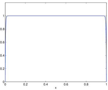
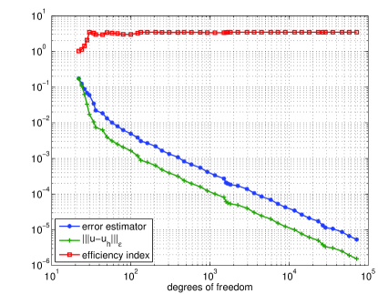
Figure 1. Example 4.7: Exact solution (left) and performance of Algorithm 4.6 (right) for $\varepsilon=10^{-5}$.

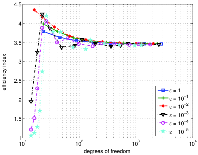
Figure 2. Example 4.7: Efficiency indices.

Example 4.8.

Furthermore, consider Fisher’s equation,

$$\varepsilon u^{\prime\prime}+u-u^{2} =0\ \text{on}\ (0,1),\qquad u_{\varepsilon}(0)=\alpha,\quad\ u_{\varepsilon}(1)=\beta.$$ (39)

A first integral form for (39) is given by $E(x,y):=\varepsilon y^{2}-\frac{2}{3}x^{3}+x^{2}$, from which we readily infer that the solutions have boundary layers close to $x=0$ and $x=1$. Furthermore, for $\alpha>-\nicefrac{{1}}{{2}}$ and $\beta<1$, the solutions feature an increasing number of spikes (which are bounded by 1) as $\varepsilon\to 0$ (see Figure 3). There are infinitely many solutions (for which there are no analytical solution formulas available in general); see, e.g., [27] for a more detailed discussion.

In our example, we have started the Newton-Raphson iteration based on a uniform grid with $100$ nodes, and an initial spike-like function depicted on the left in Figure 3. Again, we set $\theta=0.5$ in (37), and perform our experiments for $\tau=0.1$ in Algorithm 2.1, and $\varepsilon=0.00025$.

In Figure 4 we depict the performance of the error estimator. The fully adaptive Newton-Galerkin scheme converges to a numerical solution as shown on the right of Figure 3. We emphasize that our scheme is able to transport the initial function to a numerical solution which is of similar shape; in particular, it seems clear that the iteration has remained in the attractor of the solution which contains the initial guess. It is well-known that this will typically not happen for the traditional Newton scheme (with fixed step size 1), or even for a damped Newton method (with fixed step size smaller than 1); indeed, for this type of problem with $\varepsilon\ll 1$, these methods will mostly fail to converge to a bounded solution at all (see, e.g., [6]).

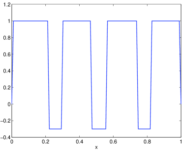
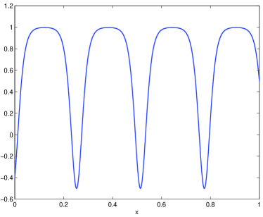
Figure 3. Example 4.8: Initial data (left) and numerical solution resulting from Algorithm 4.6 (right) with $\alpha=-0.4$, $\beta=0.5$, and $\varepsilon=0.00025$.

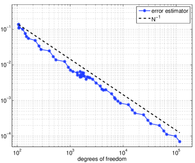
Figure 4. Example 4.8: Estimated error for $\varepsilon=0.00025$.

4.6.2. A Problem in 2d

We will now turn to a 2d-example, where we shall employ the simple prediction strategy presented in Algorithm 2.1 (see also [2]) for the selection of the local Newton-Raphson step size.

Example 4.9.

Consider the well-known nonlinear Ginzburg-Landau equation on the unit square $\Omega=(0,1)^{2}$ given by

$$\varepsilon\Delta u-u^{3}+u =0\ \text{in }\Omega,\qquad u=0\ \text{on }\partial\Omega.$$ (40)

Clearly $u\equiv 0$ is a solution. In addition, any solution $u$ appears pairwise as $-u$ is obviously a solution also. Neglecting the boundary conditions for a moment, one observes that $u\equiv 1$ and $u\equiv-1$ are solutions of the PDE. We therefore expect boundary layers along $\partial\Omega$, and possibly within the domain $\Omega$; see Figure  5, where we depict two different solutions of problem (40).

The solution on the top left in Figure 5 was obtained from choosing the initial function $(x_{1},x_{2})\mapsto\mathrm{sign}(x_{2})$, whereas the solution on the bottom left was computed by choosing $(x_{1},x_{2})\mapsto-1$ (both with enforced zero Dirichlet boundary conditions at the boundary degrees of freedom). The perturbation parameter is chosen to be $\varepsilon=0.5\cdot 10^{-5}$. We restrict the Newton step size in Algorithm 2.1 by choosing $\tau=0.1$. Moreover we have set $\theta=0.75$. Again the performance data illustrated on the right-hand side in Figure 5 indicates (optimal) first-order convergence as expected.

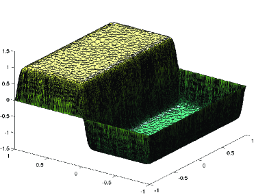
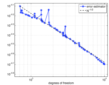
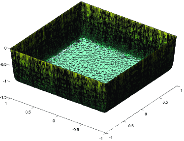
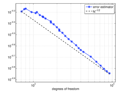
Figure 5. Example 4.9: Numerical solutions (left) and the corresponding performances (right) with $\varepsilon=0.5\cdot 10^{-5}$ for different initial guesses.

5. Conclusions

The aim of this paper was to introduce a reliable and computationally feasible procedure for the numerical solution of general, semilinear elliptic boundary value problems with possible singular perturbations. The key idea is to combine an adaptive Newton-Raphson method with an automatic mesh refinement finite element procedure. Here, the (local) Newton-Raphson damping parameter is selected based on interpreting the scheme within the context of step size control for dynamical systems. Furthermore, the sequence of linear problems resulting from the Newton discretization is treated by means of a robust (with respect to the singular perturbations) a posteriori residual-oriented error analysis and a corresponding adaptive mesh refinement scheme. Our numerical experiments clearly illustrate the ability of our approach to reliably find solutions reasonably close to the initial guesses, and to robustly resolve the singular perturbations at an optimal rate.

Appendix A A Sobolev Inequality

Lemma A.1.

Let $\Omega\subset\mathbb{R}^{d}$ be a bounded open interval ($d=1$), or a bounded Lipschitz domain ($d=2$). Then, if $g\in L^{1+\beta(d-1)}(\Omega)$, for some $\beta\in(0,1]$, then there holds that

$$\|guv\|_{L^{1}(\Omega)}\preccurlyeq\|g\|_{L^{1+\beta(d-1)}(\Omega)}\|\nabla u\|_{L^{2}(\Omega)}\|\nabla v\|_{L^{2}(\Omega)},$$

for any $u,v\in H^{1}_{0}(\Omega)$.

Proof.

We treat the cases $d=1$ and $d=2$ separately.

Case $d=1$:

By the Sobolev embedding theorem and the Poincaré inequality there holds $\left\|u\right\|_{L^{\infty}(\Omega)}\preccurlyeq\left\|\nabla{u}\right\|_{L^{2}(\Omega)}$. Thence, we get

$$\left\|guv\right\|_{L^{1}(\Omega)}\leq\left\|g\right\|_{L^{1}(\Omega)}\left\|uv\right\|_{L^{\infty}(\Omega)}\preccurlyeq\left\|g\right\|_{L^{1}(\Omega)}\left\|\nabla(uv)\right\|_{L^{2}(\Omega)}.$$ (41)

Furthermore, due to the product rule and the triangle inequality, we have

$$\begin{split}\left\|\nabla(uv)\right\|_{L^{2}(\Omega)}&\leq\left\|u\nabla{v}\right\|_{L^{2}(\Omega)}+\left\|v\nabla{u}\right\|_{L^{2}(\Omega)}\\ &\leq\left\|u\right\|_{L^{\infty}(\Omega)}\left\|\nabla{v}\right\|_{L^{2}(\Omega)}+\left\|v\right\|_{L^{\infty}(\Omega)}\left\|\nabla{u}\right\|_{L^{2}(\Omega)}\\ &\preccurlyeq\left\|\nabla u\right\|_{L^{2}(\Omega)}\left\|\nabla{v}\right\|_{L^{2}(\Omega)}.\end{split}$$ (42)

Inserting this bound into (41) completes the argument for $d=1$.

Case $d=2$:

We choose $\delta\in(0,1]$ to be specified later, and set $p(\delta):=\nicefrac{{(4-2\delta)}}{{(4-3\delta)}}\in(1,2]$ and $q(\delta):=\nicefrac{{(4-2\delta)}}{{\delta}}\in[2,\infty)$, so that $p(\delta)^{-1}+q(\delta)^{-1}=1$. Then, by means of Hölder’s inequality, we note that

$$\left\|guv\right\|_{L^{1}(\Omega)}\leq\left\|g\right\|_{L^{p(\delta)}(\Omega)}\left\|uv\right\|_{L^{q(\delta)}(\Omega)}.$$ (43)

Here, referring to [13, Theorem 3.4.3]), there holds

$$\left\|uv\right\|_{L^{q(\delta)}(\Omega)}\preccurlyeq\left\|\nabla(uv)\right\|_{L^{r(\delta)}(\Omega)},$$ (44)

with $r(\delta):=2-\delta\in[1,2)$. Using the product rule together with the triangle inequality, results in

$$\left\|\nabla{(uv)}\right\|_{L^{r(\delta)}(\Omega)}\leq\left\|u\nabla{v}\right\|_{L^{r(\delta)}(\Omega)}+\left\|v\nabla{u}\right\|_{L^{r(\delta)}(\Omega)}.$$ (45)

Then, invoking Hölder’s inequality again as well as (44), we see that

$$\left\|u\nabla{v}\right\|_{L^{r(\delta)}(\Omega)} \leq\left\|u\right\|_{L^{\nicefrac{{2r(\delta)}}{{(2-r(\delta))}}}(\Omega)}\left\|\nabla{v}\right\|_{L^{2}(\Omega)}$$ (46)

$$=\left\|u\right\|_{L^{q(\delta)}(\Omega)}\left\|\nabla{v}\right\|_{L^{2}(\Omega)}\preccurlyeq\left\|\nabla{u}\right\|_{L^{r(\delta)}(\Omega)}\left\|\nabla{v}\right\|_{L^{2}(\Omega)}$$

$$\preccurlyeq\left\|\nabla{u}\right\|_{L^{2}(\Omega)}\left\|\nabla{v}\right\|_{L^{2}(\Omega)},$$

and similarly,

$$\left\|v\nabla{u}\right\|_{L^{r(\delta)}(\Omega)}\preccurlyeq\left\|\nabla{v}\right\|_{L^{2}(\Omega)}\left\|\nabla{u}\right\|_{L^{2}(\Omega)}.$$ (47)

Combining (43)–(47), we end up with

$$\|guv\|_{L^{1}(\Omega)}\preccurlyeq\|g\|_{L^{p(\delta)}(\Omega)}\|\nabla u\|_{L^{2}(\Omega)}\|\nabla v\|_{L^{2}(\Omega)},$$

which shows the claim with $p(\delta)=1+\beta\in(1,2]$. ∎

References

- [1] A. Ambrosetti and A. Malchiodi, Perturbation methods and semilinear elliptic problems on , Progress in Mathematics, vol. 240, Birkhäuser Verlag, Basel, 2006.
- [2] M. Amrein and T. P. Wihler, An adaptive Newton-method based on a dynamical systems approach, Commun. Nonlinear Sci. Numer. Simul. 19 (2014), no. 9, 2958–2973.
- [3] G. Barles and J. Burdeau, The Dirichlet problem for semilinear second-order degenerate elliptic equations and applications to stochastic exit time control problems, Comm. Partial Differential Equations 20 (1995), no. 1-2, 129–178.
- [4] H. Berestycki and P.-L. Lions, Nonlinear scalar field equations. I. Existence of a ground state, Arch. Rational Mech. Anal. 82 (1983), no. 4, 313–345.
- [5] R. S. Cantrell and C. Cosner, Spatial ecology via reaction-diffusion equations, Wiley Series in Mathematical and Computational Biology, John Wiley & Sons, Ltd., Chichester, 2003.
- [6] G. Chen, J. Zhou, and W.-M. Ni, Algorithms and visualization for solutions of nonlinear elliptic equations, Internat. J. Bifur. Chaos Appl. Sci. Engrg. 10 (2000), no. 7, 1565–1612.
- [7] P. Deuflhard, Newtons method for nonlinear problems, Springer Ser. Comput. Math., 2004.
- [8] M. Drexler, I. J. Sobey, and C. Bracher, On the fractal characteristics of a stabilised Newton method, Tech. Report NA-95/26, Computing Laboratory, Oxford University, 1995.
- [9] L. Edelstein-Keshet, Mathematical models in biology, Classics in Applied Mathematics, vol. 46, Society for Industrial and Applied Mathematics (SIAM), Philadelphia, PA, 2005, Reprint of the 1988 original.
- [10] B. I. Epureanu and H. S. Greenside, Fractal basins of attraction associated with a damped Newton’s method, SIAM Review 40 (1998), no. 1, 102–109.
- [11] A. Ern and M. Vohralík, Adaptive inexact Newton methods with a posteriori stopping criteria for nonlinear diffusion PDEs, SIAM J. Sci. Comput. 35 (2013), no. 4, A1761–A1791.
- [12] A. Friedman (ed.), Tutorials in mathematical biosciences. IV, Lecture Notes in Mathematics, vol. 1922, Springer, Berlin; MBI Mathematical Biosciences Institute, Ohio State University, Columbus, OH, 2008, Evolution and ecology, Mathematical Biosciences Subseries.
- [13] J. Jost and X. Li-Jost, Calculus of variations, Cambridge Studies in Advanced Mathematics, vol. 64, Cambridge University Press, Cambridge, 1998.
- [14] J. M. Melenk and T. P. Wihler, A posteriori error analysis of -FEM for singularly perturbed problems, submitted (2014).
- [15] J. W. Neuberger, Continuous Newton’s method for polynomials, The Mathematical Intelligencer 21 (1999), no. 3, 18–23.
- [16] W.-M. Ni, The mathematics of diffusion, CBMS-NSF Regional Conference Series in Applied Mathematics, vol. 82, Society for Industrial and Applied Mathematics (SIAM), Philadelphia, PA, 2011.
- [17] A. Okubo and S. A. Levin, Diffusion and ecological problems: modern perspectives, second ed., Interdisciplinary Applied Mathematics, vol. 14, Springer-Verlag, New York, 2001.
- [18] H.-O. Peitgen and P. H. Richter, The beauty of fractals, Springer Verlag, 1986.
- [19] P. H. Rabinowitz, Minimax methods in critical point theory with applications to differential equations, CBMS Regional Conference Series in Mathematics, vol. 65, Published for the Conference Board of the Mathematical Sciences, Washington, DC; by the American Mathematical Society, Providence, RI, 1986.
- [20] H.-G. Roos, M. Stynes, and L. Tobiska, Robust numerical methods for singularly perturbed differential equations, second ed., Springer Series in Computational Mathematics, vol. 24, Springer-Verlag, Berlin, 2008, Convection-diffusion-reaction and flow problems.
- [21] H. R. Schneebeli and T. P. Wihler, The Newton-Raphson method and adaptive ODE solvers, Fractals 19 (2011), no. 1, 87–99.
- [22] S. Smale, On the efficiency of algorithms of analysis, Bull. Amer. Math. Soc. (N.S.) 13 (1985), no. 2, 87–121.
- [23] J. Smoller, Shock waves and reaction-diffusion equations, second ed., Grundlehren der Mathematischen Wissenschaften [Fundamental Principles of Mathematical Sciences], vol. 258, Springer-Verlag, New York, 1994.
- [24] W. A. Strauss, Existence of solitary waves in higher dimensions, Comm. Math. Phys. 55 (1977), no. 2, 149–162.
- [25] R. Verfürth, Robust a posteriori error estimators for a singularly perturbed reaction-diffusion equation, Numer. Math. 78 (1998), no. 3, 479–493.
- [26] R. Verfürth, A posteriori error estimation techniques for finite element methods, Numerical Mathematics and Scientific Computation, Oxford University Press, Oxford, 2013.
- [27] F. Verhulst, Methods and applications of singular perturbations, Texts in Applied Mathematics, vol. 50, Springer, New York, 2005, Boundary layers and multiple timescale dynamics.