Electroweak prodution of top-quark pairs in $e^{+}e^{-}$ annihilation at NNLO in QCD: the vector contributions

Abstract

We report on a calculation of the vector current contributions to the electroweak production of top quark pairs in $e^{+}e^{-}$ annihilation at next-to-next-to-leading order in Quantum Chromodynamics. Our setup is fully differential and can be used to calculate any infrared-safe observable. The real emission contributions are handled by a next-to-next-to-leading order generalization of the phase-space slicing method. We demonstrate the power of our technique by considering its application to various inclusive and exclusive observables.

1 Introduction

Continuum electroweak production of top quark pairs at future linear colliders is of considerable interest because it allows for a precise measurement of the top quark forward-backward asymmetry. This observable is of particular importance because it is expected to severely constrain anomalous couplings which could potentially appear in the top quark sector hep-ex/0509008 . In the near future, due to the extremely clean environment expected at proposed $e^{+}e^{-}$ colliders, it should be possible to measure the top quark forward-backward asymmetry to a precision of approximately $1\%$ 1005.1756 .

At an $e^{+}e^{-}$ collider, top quark pairs are primarily produced via the electroweak process

$$e^{+}e^{-}\to\gamma^{*}/Z^{*}\to t\bar{t}\,.$$ (1)

In this paper, we shall only concern ourselves with the next-to-next-to-leading order (NNLO) radiative corrections to the above process in Quantum Chromodynamics (QCD) mediated by an off-shell photon ($\gamma^{*}$). In other words, we treat the vector current contributions to the production of a top-antitop pair. Complete results including the axial-vector contributions (i.e. that due to off-shell $Z$ boson exchange) will be presented elsewhere.

The calculation of QCD radiative corrections to heavy-quark pair production in $e^{+}e^{-}$ annihilation has a long history. Full next-to-leading order (NLO) QCD corrections were first computed in ref. PHRVA.D25.1218 and, a short time later, NLO electroweak effects were considered in ref. NUPHA.B365.24 . NLO QCD corrections to top quark pair production including the subsequent top quark decays were presented in ref. Schmidt:1995mr and NLO QCD corrections to top quark spin correlations were computed in refs. hep-ph/9807209 and hep-ph/9901205 . Total cross sections are known to NNLO in the threshold expansions hep-ph/9712222 ; hep-ph/9712302 ; hep-ph/9801397 ; hep-ph/0001286 ; hep-ph/9508274 and high-energy expansions Gorishnii:1986pz ; PHLTA.B248.359 ; hep-ph/9406299 ; hep-ph/9710413 ; hep-ph/9704222 . Results for the forward-backward asymmetry are also known in the small mass approximation NUPHA.B391.3 ; hep-ph/9809411 ; hep-ph/9905424 . In the near future, the threshold cross section at NNNLO will also be available Beneke:2013jia ; Marquard:2014pea ; Beneke:2014qea . Somewhat surprisingly, although a great deal of theoretical progress has been made over the years, exact NNLO QCD calculations for fully differential $e^{+}e^{-}\to t\bar{t}$ observables remain a challenge and are still missing from the literature.

A fully differential NNLO QCD calculation is naturally split up into three distinct parts, depending on the number of particles that appear in the final state relative to leading order: a) purely virtual two-loop or squared one-loop corrections, b) one-loop, single-emission real-virtual corrections, and c) double-emission double-real corrections. For $e^{+}e^{-}\to t\bar{t}$, significant progress has been made in recent years towards the calculation of each of these three pieces. NLO QCD corrections to heavy quark pair production in association with one additional jet were computed in refs. hep-ph/9703358 ; hep-ph/9705295 ; hep-ph/9708350 ; hep-ph/9709360 ; hep-ph/9905276 . The two-loop heavy quark form factor was first obtained in refs. hep-ph/0406046 ; hep-ph/0412259 ; hep-ph/0504190 and then confirmed some time later by an independent calculation 0905.1137 . In fact, for quite some time, the only outstanding problem was to construct an efficient framework for the combination of the ingredients described above into an infrared-safe Monte Carlo event generator.

For generic processes, this is highly non-trivial due to the fact that, in phase space regions where soft and/or collinear limits are approached, the real-virtual and double-real contributions develop soft and/or collinear divergences which must be extracted before a Monte Carlo integration over phase space can be carried out. At NLO, this is relatively straightforward to do and both phase-space slicing Fabricius:1981sx ; Kramer:1986mc ; Baer:1989jg ; PHRVA.D46.1980 ; hep-ph/9302225 ; hep-ph/0102128 ; Keller:1998tf and subtraction Ellis:1980wv ; Mangano:1991jk ; Kunszt:1992tn ; hep-ph/9512328 ; hep-ph/9605323 ; hep-ph/0201036 techniques which solve the problem were worked out long time ago. However, as is clear from the massive amount of literature on the subject hep-ph/0004013 ; hep-ph/0302180 ; hep-ph/0306248 ; hep-ph/0311311 ; hep-ph/0402265 ; hep-ph/0402280 ; hep-ph/0403057 ; hep-ph/0409088 ; hep-ph/0411399 ; hep-ph/0502226 ; hep-ph/0505111 ; hep-ph/0603182 ; hep-ph/0609042 ; hep-ph/0609043 ; hep-ph/0703012 ; 0710.0346 ; 0802.0813 ; 0807.0509 ; 0807.3241 ; PHLTA.B666.336 ; 0807.0514 ; 0903.2120 ; 0904.1145 ; 0905.4390 ; 0912.0374 ; 1003.2824 ; JHEPA.1002.089 ; 1003.4451 ; 1005.0274 ; 1011.1909 ; 1011.6631 ; 1101.0642 ; 1105.0530 ; 1107.4037 ; 1107.1164 ; 1110.2368 ; 1110.2375 ; 1112.4736 ; 1204.5201 ; 1207.5779 ; 1207.6546 ; 1210.2808 ; 1210.5059 ; 1301.4693 ; 1301.7133 ; 1301.7310 ; 1302.6216 ; 1303.6254 ; 1309.6887 ; 1309.7000 ; 1310.3993 ; 1401.7754 ; 1404.6493 ; 1404.7116 ; 1405.2219 ; Anastasiou:2014nha , analogous techniques at NNLO are considerably more complicated to develop and complete solutions took much longer to emerge. For example, in the important case of massless dijet production, it took more than a decade for the first physical predictions to appear 1301.7310 ; 1310.3993 from the time that the relevant two-loop virtual amplitudes were first calculated hep-ph/0001001 ; hep-ph/9905323 ; hep-ph/9909506 ; hep-ph/0003261 ; hep-ph/0010212 ; hep-ph/0011094 ; hep-ph/0012007 ; hep-ph/0101304 ; hep-ph/0102201 ; hep-ph/0104178 . As a result of significant theoretical efforts during the past decade, a number of important “benchmark processes” are now known to NNLO 1204.5201 ; 1301.7310 ; 1302.6216 ; 1303.6254 ; 1310.3993 ; 1405.2219 .

The goal of this paper is to study fully differential NNLO QCD corrections to $e^{+}e^{-}\to t\bar{t}$ using a higher-order generalization of the phase-space slicing method. While we constrain ourselves in this paper to present results for the vector current contributions by themselves, the formalism developed here can, if desired, readily be used to calculate the contributions coming from the exchange of an off-shell $Z$ boson. This paper is organized as follows. In Section 2, we describe our calculational method in detail. In Section 3, we present numerical results for various inclusive and differential observables and, whenever possible, compare them to the existing literature. Finally, we conclude in Section 4.

2 Phase-space slicing at NNLO

We explain in detail our generalization of phase-space slicing method in dealing with the specific process $e^{+}e^{-}\to t\bar{t}$ at NNLO. As mentioned before, there are three distinct parts contribute to the cross section at ${\mathcal{O}(\alpha_{s}^{2})}$,

$$\sigma^{(2)}= \int\!\mathrm{d}\Phi_{t\bar{t},0}\sum_{\mathrm{spin,color}}\left[2\Re\left(\mathcal{M}^{(0)}_{e^{+}e^{-}\to t\bar{t}}\left(\mathcal{M}^{(2)}_{e^{+}e^{-}\to t\bar{t}}\right)^{*}\right)+\left|\mathcal{M}^{(1)}_{e^{+}e^{-}\to t\bar{t}}\right|^{2}\right]$$

$$+\int\!\mathrm{d}\Phi_{t\bar{t},1}\sum_{\mathrm{spin,color}}\left[2\Re\left(\mathcal{M}^{(0)}_{e^{+}e^{-}\to t\bar{t}g}\left(\mathcal{M}^{(1)}_{e^{+}e^{-}\to t\bar{t}g}\right)^{*}\right)\right]$$

$$+\int\!\mathrm{d}\Phi_{t\bar{t},2}\sum_{\mathrm{spin,color}}\left[\left|\mathcal{M}^{(0)}_{e^{+}e^{-}\to t\bar{t}gg}\right|^{2}+\left|\mathcal{M}^{(0)}_{e^{+}e^{-}\to t\bar{t}q\bar{q}}\right|^{2}\right],$$ (2)

where

$$\mathrm{d}\Phi_{t\bar{t},n}= \frac{1}{2s\times 2^{2}}\left(\frac{\mathrm{d}^{D-1}p_{t}}{2E_{t}(2\pi)^{D-1}}\right)\left(\frac{\mathrm{d}^{D-1}p_{\bar{t}}}{2E_{\bar{t}}(2\pi)^{D-1}}\right)$$

$$\times\prod^{n}_{i=1}\left(\frac{\mathrm{d}^{D-1}p_{i}}{2E_{i}(2\pi)^{D-1}}\right)(2\pi)^{D}\delta^{(D)}\left(Q-p_{t}-p_{\bar{t}}-\sum_{i=1}^{n}p_{i}\right)$$ (3)

is the phase space volume element in $D=4-2\epsilon$ dimension, divided by the flux factor and initial state spin average factor. Here $s=Q^{2}=(p_{e^{+}}+p_{e^{-}})^{2}$ is the center-of-mass energy square. $\mathcal{M}^{(i)}_{e^{+}e^{-}\to t\bar{t}\dots}$ denotes the $i$-loop amplitude for $e^{+}e^{-}\to t\bar{t}$ plus zero, one, or two additional massless partons. Note that when $\sqrt{s}>4m_{t}$, the channel for the production of $t\bar{t}t\bar{t}$ is open. However, these additional contributions are themselves infrared finite due to the mass of top quark, and can be dealt with separately. In the following discussion, we will neglect these contributions. Also for the vector contributions, we only consider diagrams with top quarks coupling directly to photon. The diagrams with photon coupling to a bottom or light quarks and the top quark produced via gluon splitting are numerically small Hoang:1994it ; hep-ph/9605311 . Though the bottom triangle diagrams are needed and must be included to cancel the axial anomaly in the axial vector case hep-ph/9710413 ; hep-ph/0504190 .

The first, second, and third terms on the RHS of Eq.(2) represent respectively the double-virtual, real-virtual, and double-real contributions. The double-virtual contributions contain explicit quadratic poles in $\epsilon$, originating from loop corrections when the gluons are soft. Thanks to Bloch-Nordsieck and Kinoshita-Lee-Nauenberg theorem, the infrared divergences will be cancelled by those in the real-virtual and double-real contributions. However, such cancellation is non-trivial because the infrared divergences in the real-virutal and double-real contributions can only be made explicit after phase space integral. It is therefore necessary to perform the phase space integral in $D$ dimension to regulate potential infrared divergences. This fact makes the calculation of real-virtual and double-real contributions difficult.

The singular region in the phase space is relatively simple for the real-virtual corrections, where the matrix elements are singular only when the energy of the final state gluon approaches zero. For the double-real contributions the singular region is much more involved. First, the matrix elements are singular in the double un-resolved region, where the energies of both the final state partons approach zero. Second, the matrix elements are also singular even in the single un-resolved region, where only one of the final state gluon is soft, or the final state massless partons become collinear. Fortunately, the singularities due to single un-resolved region is well understood, as they are the same one encounters in NLO QCD calculation. We therefore only need to deal with the double un-resolved region. To isolate the phase space singularities in this region, we introduce a phase-space slicing parameter $\tau$, which is proportional to the total energy of QCD radiations in the final state, $\tau=2(\sqrt{s}-(E_{t}+E_{\bar{t}}))/(\sqrt{s}(1-4m^{2}_{t}/s))$. Physically, when $\tau$ is non-zero, there is at least one massless parton in the final state with finite energy. We can divide the phase space into two slices using the theta function,

$$\sigma^{(2)}=\sigma^{(2)}_{I}+\sigma^{(2)}_{II},$$ (4)

where $\sigma^{(2)}_{I}=\int\!\mathrm{d}\sigma\theta(\delta_{E}-\tau)$ is the soft-virtual part, and $\sigma^{(2)}_{II}=\int\!\mathrm{d}\sigma\theta(\tau-\delta_{E})$ is the hard part, and $\delta_{E}$ is the cut-off parameter. There are still phase space singularities in both $\sigma_{I}$ and $\sigma_{II}$. However, the phase space singularties in $\sigma_{II}$ belong to the well understood one, because there is at most one massless parton in the final state whose energy can approach zero. We can therefore straight-forwardly calculate $\sigma_{II}$ using any existing NLO infrared subtraction method. On the other hand, the soft-virtual part, $\sigma_{I}$, contains double un-resolved region, whose calculation needs additional efforts. An exact calculation for $\sigma_{I}$ is difficult. However, if we choose $\delta_{E}$ to be small and ignore terms of ${\mathcal{O}(\delta_{E})}$, we can calculate $\sigma_{I}$ using matrix elements in the soft limit, and also expanding the phase space volume in the soft limit. Such approximation leads to enormous simplification and makes the analytical calculation feasible. We explain in detail the calculation of the soft-virtual part and hard part below.

2.1 The soft-virtual part

2.1.1 Factorization of the radiation-energy distribution

We can write the soft-virtual part as an integral over radiation-energy distribution,

$$\sigma^{(2)}_{I}=\int^{\delta_{E}}_{0}\!\mathrm{d}\tau\frac{\mathrm{d}\omega}{\mathrm{d}\tau}\frac{\mathrm{d}\sigma^{(2)}}{\mathrm{d}\omega},$$ (5)

where $\omega$ is twice the energy of final state QCD radiations, $\omega=2(\sqrt{s}-E_{t}-E_{\bar{t}})$. The factor of $2$ here is introduced by convention. Ignoring power suppressed terms in $\omega/m_{t}$, we can write the distribution for $\mathrm{d}\sigma/\mathrm{d}\omega$ in small $\omega$ in a factorized form using the language of effective theory. $\mathrm{d}\sigma^{(2)}/\mathrm{d}\omega$ is simply the order ${\mathcal{O}(\alpha_{s}^{2})}$ corrections to this distribution. We start from the full distribution in QCD,

$$\frac{\mathrm{d}\sigma}{\mathrm{d}\omega}=\sum_{t,\bar{t},X}(2\pi)^{4}\delta^{(4)}(Q-p_{t}-p_{\bar{t}}-p_{X})\delta(\omega-2E(X))L_{\mu\nu}\sum_{ij}\langle 0|J^{\mu}_{i}|t\bar{t}X\rangle\langle t\bar{t}X|J^{\nu}_{j}|0\rangle\ ,$$ (6)

where $X$ denotes gluons and light quarks in the final state. $E(X)$ denotes the energy of $X$. The lepton tensor includes only vector contributions from virtual photon exchange,

$$L_{\mu\nu}=-\frac{2e^{2}}{s}\left(g_{\mu\nu}-\frac{2(p^{e^{+}}_{\mu}p^{e^{-}}_{\nu}+p^{e^{+}}_{\nu}p^{e^{-}}_{\mu})}{s}\right)\ ,$$ (7)

where $e$ is the QED coupling, and $p^{e^{+}}_{\mu}$ and $p^{e^{-}}_{\mu}$ are the four momentum of positron and electron. The production of top-quark pair via virtual photon exchange is described by two QCD currents,

$$J^{\mu}_{1}=-ieQ_{t}\bar{u}(p_{t})\gamma^{\mu}v(p_{\bar{t}}),\qquad J^{\mu}_{2}=\frac{eQ_{t}}{2m_{t}}\bar{u}(p_{t})\sigma^{\mu\nu}(p_{t}+p_{\bar{t}})_{\nu}v(p_{\bar{t}})\ ,$$ (8)

where $Q_{t}=2/3$ is the electric charge number of top quark, and $\sigma^{\mu\nu}=\frac{i}{2}[\gamma^{\mu},\gamma^{\nu}]$. Note that Eq. (6) is exact to leading order in electroweak interaction, and all orders in QCD interactions. It is also an exact distributions for $\omega$. Calculation of Eq. (6) in perturbative QCD requires the calculation of both virtual corrections and phase space integral. Unfortunately, exact calculation of phase space integral is difficult beyond NLO. Certain approximation is needed in order to proceed. Since we are only interested in the energy distribution in the soft region, we can expand Eq. (6) to leading power in $\omega/m_{t}$. Then the momentum conservation delta function factorizes as

$$\sum_{t,\bar{t},X}(2\pi)^{4}\delta^{(4)}(Q-p_{t}-p_{\bar{t}}-p_{X})\simeq\sum_{t,\bar{t}}(2\pi)^{4}\delta^{(4)}(Q-p_{t}-p_{\bar{t}})\sum_{X}$$ (9)

in the region where $\Lambda_{QCD}\ll\omega\ll m_{t}$. The physics of such factorization is that as long as the energy of QCD radiations is small, they can hardly change the trajectory of heavy quark. The short-distance interaction which produces the top-quark pair can not resolve the activities of soft QCD radiations, therefore have tree-level like kinematics. We can describe the top quark and antitop quark by heavy quark fields $h_{v}(y)$ and $h_{\bar{v}}(y)$, labeled by the velocity of the heavy quarks, $p_{t}=m_{t}v$, $p_{\bar{t}}=m_{t}\bar{v}$. The QCD currents in Eq. (8) can then be matched to currents in Heavy Quark Effective Theory (HQET),

$$\mathcal{J}^{\mu}_{1}=-ieQ_{t}C_{1}(v,\bar{v})\bar{h}_{v}\gamma^{\mu}h_{\bar{v}},\qquad\mathcal{J}^{\mu}_{2}=\frac{eQ_{t}}{2}C_{2}(v,\bar{v})\bar{h}_{v}\sigma^{\mu\nu}(v+\bar{v})_{\nu}h_{\bar{v}}\ ,$$ (10)

where the corresponding Wilson coefficients $C_{1}(v,\bar{v})$ and $C_{2}(v,\bar{v})$ can be obtained from the calculation of QCD form factor for heavy quark pair production. At leading power in HQET, the heavy quark field only interacts with gluons via eikonal interaction,

$$\mathcal{L}_{int}=\bar{h}_{v}(y)gv\cdot A_{s}(y)h_{v}(y)+\bar{h}_{\bar{v}}(y)g\bar{v}\cdot A_{s}(y)h_{\bar{v}}(y)$$ (11)

Such eikonal interactions can be absorbed into Wilson lines by a field redefinition hep-ph/0109045 ,

$$(h_{v}(y))^{\dagger}=(h^{(0)}_{v}(y))^{\dagger}(Y_{v}(y))^{\dagger},\qquad h_{\bar{v}}(y)=Y_{\bar{v}}(y)h^{(0)}_{\bar{v}}(y)\ ,$$ (12)

where

$$(Y_{v}(y))^{\dagger}= \mathbf{P}\exp\left(ig\int^{\infty}_{0}\mathrm{d}z\cdot A(vz+y)\right)$$

$$Y_{\bar{v}}(y)= \overline{\mathbf{P}}\exp\left(-ig\int^{\infty}_{0}\mathrm{d}z\cdot A(\bar{v}z+y)\right)$$ (13)

are the path-ordered and anti path-ordered Wilson lines. The decoupled heavy quark field $h^{(0)}_{v}(x)$ no longer interacts with gluon, but still annihilate the top quark field. The hadronic tensor now has a factorized form,

$$\sum_{X}\delta(\omega-2E(X))\sum_{ij}\langle 0|\mathcal{J}^{\mu}_{i}|t\bar{t}X\rangle\langle t\bar{t}X|\mathcal{J}^{\nu}_{j}|0\rangle=H^{\mu\nu}\sum_{X}\langle 0|Y_{v}^{\dagger}Y_{\bar{v}}|X\rangle\delta(\omega-2E(X))\langle X|Y_{\bar{v}}^{\dagger}Y_{v}|0\rangle$$ (14)

$H^{\mu\nu}$ is the hard function,

$$H^{\mu\nu}=\sum_{i,j=1}^{2}\langle 0|\mathcal{J}^{(0),\mu}_{i}|t\bar{t}\rangle\langle t\bar{t}|\mathcal{J}^{(0),\nu}_{j}|0\rangle\ ,$$ (15)

and $\mathcal{J}^{(0),\mu}_{i}$ is the decoupled HQET current, with $h_{v,\bar{v}}(y)$ replaced by $h_{v,\bar{v}}^{(0)}(y)$. Summing over the top quark spin and color , the hard function can be evaluated explictly,

$$H^{\mu\nu}=N_{c}\sum_{i,j=1}^{2}C_{i}(v,\bar{v})C_{j}^{*}(v,\bar{v})h^{\mu\nu}_{ij},$$ (16)

with

$$h^{\mu\nu}_{11}= e^{2}Q^{2}_{t}\left(-2sg^{\mu\nu}+4(p^{\mu}_{t}p^{\nu}_{\bar{t}}+p^{\nu}_{t}p^{\mu}_{\bar{t}})\right)\ ,$$ (17)

$$h^{\mu\nu}_{12}= h^{\mu\nu}_{21}=2e^{2}Q^{2}_{t}\left(-sg^{\mu\nu}+(p^{\mu}_{t}+p^{\mu}_{\bar{t}})(p^{\nu}_{t}+p^{\nu}_{\bar{t}})\right)\ ,$$ (18)

$$h^{\mu\nu}_{22}= e^{2}Q^{2}_{t}\left(-2sg^{\mu\nu}+\left(2-\frac{s}{2m^{2}_{t}}\right)(p^{\mu}_{t}p^{\nu}_{\bar{t}}+p^{\nu}_{t}p^{\mu}_{\bar{t}})+\left(2+\frac{s}{2m^{2}_{t}}\right)(p^{\mu}_{t}p^{\nu}_{t}+p^{\mu}_{\bar{t}}p^{\nu}_{\bar{t}})\right)$$ (19)

$N_{c}=3$ is the number of color in QCD. The matrix element of the Wilson lines defines the soft function for $t\bar{t}$ production,

$$S=\frac{1}{N_{c}}\sum_{X}\langle 0|Y_{v}^{\dagger}Y_{\bar{v}}|X\rangle\delta(\omega-2E(X))\langle X|Y_{\bar{v}}^{\dagger}Y_{v}|0\rangle\ ,$$ (20)

The summation is over all possible QCD final states. We have chosen the normalization such that at LO the soft function is $\delta(\omega)$. The calculation for soft function is much easier than the exact phase space integral, thanks to the eikonal approximation.

We can now write down a factorized formula for the radiation-energy distribution in top-quark pair production,

$$\frac{\mathrm{d}\sigma_{\mathrm{s.v.}}}{\mathrm{d}\omega}=\frac{1}{8s}\int\!\frac{d^{3}p_{t}}{2E_{t}(2\pi)^{3}}\int\!\frac{d^{3}p_{\bar{t}}}{2E_{\bar{t}}(2\pi)^{3}}(2\pi)^{4}\delta^{(4)}(Q-p_{t}-p_{\bar{t}})L_{\mu\nu}H^{\mu\nu}S(x,\omega)\ ,$$ (21)

where we have also included the initial dtate flux and spin average factor. The variable $x$ is defined as

$$x=\frac{1-\sqrt{1-\frac{4m^{2}_{t}}{s}}}{1+\sqrt{1-\frac{4m^{2}_{t}}{s}}}$$ (22)

For fixed $m_{t}$, $x\to 0$ is the high energy limit, while $x\to 1$ is the threshold limit. Eq. (21) is only valid at leading power in $\omega$. The soft function is fully differential in the top and antitop momentum, but inclusive in the QCD radiations. This is not a problem as we will use this formula only in the limit of small $\omega$, where the QCD radiations can not be resolved by any reasonable experimental measurement.

The phase space integral in Eq. (21) becomes trivial. Integrating out the azimuthal angle dependence of top quark, we obtain

$$\frac{\mathrm{d}^{2}\sigma_{\mathrm{s.v.}}}{\mathrm{d}\omega\,\mathrm{d}\cos\theta_{t}}=\mathcal{H}(\cos\theta_{t},m_{t},s)S(x,\omega)\ ,$$ (23)

where

$$\mathcal{H}(\cos\theta_{t},m_{t},s)= \frac{1}{8s}\int\!\frac{d^{3}p_{t}}{2E_{t}(2\pi)^{3}}\int\!\frac{d^{3}p_{\bar{t}}}{2E_{\bar{t}}(2\pi)^{3}}$$

$$\times(2\pi)^{4}\delta^{(4)}(Q-p_{t}-p_{\bar{t}})\delta\left(\cos\theta_{t}-\frac{{\boldsymbol{p}}_{t}\cdot{\boldsymbol{p}}_{e}}{|{\boldsymbol{p}}_{t}||{\boldsymbol{p}}_{e}|}\right)L_{\mu\nu}H^{\mu\nu}$$ (24)

The soft function is a distribution in $\omega$. It is often convenient to perform a Laplace transformation,

$$\frac{\mathrm{d}^{2}\tilde{\sigma}_{\mathrm{s.v.}}}{d\kappa\,\mathrm{d}\cos\theta_{t}}= \int^{\infty}_{0}\!\mathrm{d}\omega\exp\left(-\frac{\omega}{e^{\gamma_{E}}\kappa}\right)\frac{\mathrm{d}^{2}\sigma_{\mathrm{s.v.}}}{\mathrm{d}\omega\,\mathrm{d}\cos\theta_{t}}$$

$$\equiv \mathcal{H}(\cos\theta_{t},m_{t},s)\tilde{s}(x,L_{\kappa})\ ,$$ (25)

where $L_{\kappa}=\ln(\kappa/\mu)$. The renormalized soft function depends on $\kappa$ only through terms of the form $L^{n}_{\kappa}$, where $n$ is a positive integer. It is therefore possible to invert the Laplace transformation in close form hep-ph/0607228 ,

$$\frac{\mathrm{d}^{2}\sigma_{\mathrm{s.v.}}}{\mathrm{d}\tau\,\mathrm{d}\cos\theta_{t}}=\mathcal{H}(\cos\theta_{t},m_{t},s)\lim_{\eta\to 0}\left[\tilde{s}\left(\partial_{\eta}\right)\left(\frac{\mu}{\sqrt{s}(1-4m^{2}_{t}/s)}\right)^{\eta}\frac{1}{\tau^{1+\eta}}\frac{\exp(-\gamma_{E}\eta)}{\Gamma(\eta)}\right]\ ,$$ (26)

where we recall that $\tau=\omega/(\sqrt{s}(1-4m^{2}_{t}/s))$. Eq. (26) is interpreted as first expanding in $\eta$ as a taylor series within the square bracket, using the well-known plus-distribution expansion

$$\frac{1}{\tau^{1+\eta}}=-\frac{\delta(\tau)}{\eta}+\frac{1}{[\tau]_{+}}-\eta\left[\frac{\ln\tau}{\tau}\right]_{+}+\mathcal{O}(\eta^{2})\ ,$$ (27)

then taking the $\eta\to 0$ limit.

2.1.2 Hard function from QCD heavy quark form factor

The Wilson coefficients defined in Eq. (10) can be obtained from the QCD heavy quark form factor. The latter has been computed for the vector contributions, axial contributions, and anomaly contributions by Bernreuther et.al hep-ph/0406046 ; hep-ph/0412259 ; hep-ph/0504190 . The vector contributions have been computed independently later in ref. 0905.1137 , confirming previous results.

In ref. hep-ph/0406046 , the vector contributions to heavy quark form factor are given to two loops in QCD. The results are expressed in terms of two dimensionless scalar form factors, $\hat{F}_{1}(x)$ and $\hat{F}_{2}(x)$,

$$-ieQ_{t}\bar{u}(p_{t})\left(\hat{F}_{1}(x)\gamma^{\mu}+\frac{1}{2m_{t}}\hat{F}_{2}(x)i\sigma^{\mu\nu}(p^{t}_{\nu}+p^{\bar{t}}_{\nu})\right)v(p_{\bar{t}})$$ (28)

Here the scalar form factors are related to those computed in Eq. (57) and (58) of ref. hep-ph/0406046 by an additional renormalization,

$$\hat{F}_{i}(x,\alpha_{s}^{N_{l}})=F_{i}(x,\alpha_{s}^{N_{f}}(\alpha_{s}^{N_{l}}))\ ,\qquad i=1,2\ ,$$ (29)

where

$$\alpha_{s}^{N_{f}}(\alpha_{s}^{N_{l}})=\alpha_{s}^{N_{l}}\left[1+\frac{8}{3}T_{R}N_{h}\frac{\alpha_{s}^{N_{l}}}{4\pi}\left(-\frac{1}{2}L_{H}+\epsilon\left(\frac{L^{2}_{H}}{4}+\frac{1}{24}\pi^{2}\right)\right)+\frac{\epsilon}{12}\left(\frac{\alpha_{s}^{N_{l}}}{4\pi}\right)\beta^{(N_{f})}_{0}\pi^{2}\right]\ ,$$ (30)

with $N_{f}=N_{l}+N_{h}$. $N_{l}=5$ is the number of light quark flavor, and $N_{h}=1$ is the number of heavy quark flavor. $T_{R}=1/2$ in QCD, $L_{H}=\ln(m^{2}_{t}/\mu^{2})$. The QCD beta function for $N_{f}$ quark flavor is given by

$$\beta^{(N_{f})}_{0}=\frac{11}{3}C_{A}-\frac{4}{3}T_{R}(N_{l}+N_{h})$$ (31)

where $C_{A}=3$ in QCD. Unless otherwise specified, we will denote $\alpha_{s}^{N_{l}}$ as $\alpha_{s}$ below. Note that $\hat{F}_{i}(x)$ and $F_{i}(x)$ only differ starting from two loops. The origin for such difference is that in ref. hep-ph/0406046 , the renormalization of strong coupling is performed in $\overline{\mathrm{MS}}$ scheme, running with $N_{f}$ flavors. Also the authors of ref. hep-ph/0406046 include a factor $\Gamma(1+\epsilon)\exp(\epsilon\gamma_{E})$ in the coupling renormalization, where $\Gamma(z)$ is Euler’s Gamma function, and $\gamma_{E}=0.577216\dots$. However, we choose to perform the calculation with $\alpha_{s}$ running with $N_{l}$ flavors, and also without the additional factor $\Gamma(1+\epsilon)\exp(\epsilon\gamma_{E})$. The decoupling of heavy quark flavor is realized by the second term on the RHS of Eq. (30) hep-ph/9411260 ; hep-ph/9706430 ; hep-ph/9708255 ; hep-ph/0004189 , while the third factor gets rid of the additional factor $\Gamma(1+\epsilon)\exp(\epsilon\gamma_{E})$ through to ${\mathcal{O}(\alpha_{s}^{2})}$ hep-ph/0612149 .

The scalar form factors are functions of $x$. Writing them as an expansion in $a_{s}=\alpha_{s}(\mu)/(4\pi)$,

$$\hat{F}_{i}(x)=\hat{F}^{(0l)}_{i}(x)+a_{s}\hat{F}^{(1l)}_{i}(x)+a^{2}_{s}\hat{F}^{(2l)}_{i}(x)+{\mathcal{O}(a^{3}_{s})}\ ,$$ (32)

we have at LO in QCD

$$\hat{F}^{(0l)}_{1}(x)=1,\qquad\hat{F}^{(0l)}_{2}(x)=0$$ (33)

Using the additional renormalization relation in Eq. (29), the one-loop and two-loop form factors can be read off from ref. hep-ph/0406046 . These form factors are UV finite but IR divergent. To calculate the Wilson coefficients defined in Eq. (10), one needs to calculate the form factors in the effective theory. The wilson coefficients are simply the differences of the form factor in QCD and the form factor in effective theory. In dimensional regularization with external state onshell, the form factors in the effective theory at one loop and beyond vanish because they invlove only scaleless integral. Since the IR divergences in the QCD calculation and effective theory calculation must match, it implies that the UV divergences in the effective theory calculation are exactly the negative of the IR divergence in the QCD calculation. Therefore, renormalization of the UV divergences in the effective theory is simply amount to performing an IR subtraction to the form factor in QCD,

$$C_{i}(x)=\lim_{\epsilon\to 0}\left[Z_{H,i}\hat{F}_{i}(x)\right]\ ,\qquad i=1,2\ ,$$ (34)

where the IR subtraction factor is defined such that $C_{i}(x)$ is order by order finite, i.e., $Z_{H,i}$ absorbs only the $\epsilon$ poles in $\hat{F}_{i}(x)$. For the convenience of reader, we give below the explicit expression for $C_{i}(x)$ at one loop, as derived from the QCD form factors in ref. hep-ph/0406046 . We have checked that using ref. 0905.1137 , we get the same Wilson coefficients.

The one-loop Wilson coefficients are

$$C^{(1l)}_{1}(x)= C_{F}\left[L_{H}\left(\left(\frac{2}{x+1}-\frac{2}{x-1}-2\right)H(0,x)+2\right)+\left(-\frac{4}{x+1}+\frac{2}{x-1}+3\right)H(0,x)\right.$$

$$\left.+\left(-\frac{2}{x+1}+\frac{2}{x-1}+2\right)H(0,0,x)+\left(-\frac{4}{x+1}+\frac{4}{x-1}+4\right)H(1,0,x)\right.$$

$$\left.-\frac{8\zeta_{2}}{x-1}+\frac{8\zeta_{2}}{x+1}-4(2\zeta_{2}+1)\right]+i\pi C_{F}\left[L_{H}\left(\frac{2}{x+1}-\frac{2}{x-1}-2\right)\right.$$

$$\left.+\left(-\frac{2}{x+1}+\frac{2}{x-1}+2\right)H(0,x)+\left(-\frac{4}{x+1}+\frac{4}{x-1}+4\right)H(1,x)\right.$$

$$\left.+\frac{2}{x-1}-\frac{4}{x+1}+3\right]$$ (35)

$$C^{(1l)}_{2}(x)= 2C_{F}\left(-\frac{1}{x-1}-\frac{1}{x+1}\right)(H(0,x)+i\pi)\ ,$$ (36)

where $C_{F}=4/3$ in QCD. The imaginary part in the Wilson coefficients results from analytical continuation of the form factors from spacelike to timelike kinematics. The function $H(\vec{w},x)$ is harmonic polylogarithm (HPL) introduced in ref. hep-ph/9905237 . We use hplog hep-ph/0107173 for the numerical calculation of HPLs in this work. The Mathematica file for the two-loop Wilson coefficients can be found in the arXiv submission of this paper.

2.1.3 Perturbative expansion of the radiation-energy distribution through to NNLO

To expand the equation for radiation-energy distribution in Eq. (26) in $\alpha_{s}$, we also need the soft function to NNLO, which have been computed only recently vMSZ . The Laplace transformed soft function has the generic form

$$\widetilde{s}(x,L_{\kappa}) = 1+a_{s}\Big{(}L_{\kappa}\,\gamma^{s}_{0}(x)+c_{1}(x)\Big{)}+a_{s}^{2}\bigg{[}L_{\kappa}^{2}\left(\frac{1}{2}\Big{(}\gamma^{s}_{0}(x)\Big{)}^{2}-\beta_{0}\gamma^{s}_{0}(x)\right)$$ (37)

$$+L_{\kappa}\left(c_{1}(x)\Big{(}\gamma^{s}_{0}(x)-2\beta_{0}\Big{)}+\gamma^{s}_{1}(x)\right)+c_{2}(x)\bigg{]}+\mathcal{O}\left(a^{3}_{s}\right).$$

through to ${\mathcal{O}(\alpha_{s}^{2})}$, where $\beta_{0}$ is the LO QCD beta function with $N_{l}$ light flavour only,

$$\beta_{0}=\frac{11}{3}C_{A}-\frac{4}{3}T_{R}N_{l}\ ,$$ (38)

and $\gamma_{0}^{s}(x)$ and $\gamma_{1}^{s}(x)$ are the well-known cusp anomalous dimension NUPHA.B283.342 ; 0903.2561 ; 0904.1021 . We reproduce them here for the sake of completeness

$$\gamma^{s}_{0}(x)=-8C_{F}\left[1+\frac{1+x^{2}}{1-x^{2}}H(0,x)\right]$$ (39)

$$\gamma^{s}_{1}(x)=\frac{160}{9}C_{F}N_{l}T_{R}\left[1+\frac{1+x^{2}}{1-x^{2}}H(0,x)\right]$$ (40)

$$+C_{A}C_{F}\left[-\frac{392}{9}+16\zeta_{2}\frac{1+9x^{2}}{1-x^{2}}+16\frac{\left(1+x^{2}\right)^{2}}{\left(1-x^{2}\right)^{2}}\Big{(}2H(0,x)\Big{(}H(0,-1,x)-H(0,1,x)\Big{)}\right.$$

$$\left.-4H(0,0,-1,x)+4H(0,0,1,x)-\zeta(3)\Big{)}+32\frac{1+x^{2}}{1-x^{2}}\bigg{(}H(0,x)\left(H(-1,x)-H(1,x)-\frac{67}{36}\right)\right.$$

$$\left.-H(0,-1,x)+H(0,1,x)\bigg{)}-\frac{32}{3}\frac{x^{2}(1+x^{2})}{\left(1-x^{2}\right)^{2}}H^{3}(0,x)-\frac{32x^{2}}{1-x^{2}}H^{2}(0,x)\right.$$

$$\left.+16\zeta_{2}\frac{\left(1+x^{2}\right)\left(1+9x^{2}\right)}{\left(1-x^{2}\right)^{2}}H(0,x)\right].$$

The soft function is largely fixed by the renormalization group equation it obeys NUPHA.B283.342 . The genuine two-loop corrections to the soft function are summarized by the scalar function $c_{2}(x)$, which is first computed in ref. vMSZ  . With all these results at hand, we can write down the radiation-energy distribution through to NNLO, up to power-correction terms in $\tau$. Writing $\mathcal{H}(\cos\theta_{t},m_{t},s)$ as an expansion in $a_{s}$, $\mathcal{H}(\cos\theta_{t},m_{t},s)=\mathcal{H}_{0}+a_{s}\mathcal{H}_{1}+a_{s}^{2}\mathcal{H}_{2}+\cdots$, the results are

$$\frac{\mathrm{d}^{2}\sigma^{(1l)}_{\mathrm{s.v.}}}{\mathrm{d}\tau\,\mathrm{d}\cos\theta_{t}}= \left[(c_{1}(x)+L_{H}\gamma^{s}_{0})\mathcal{H}_{0}+\mathcal{H}_{1}\right]\delta(\tau)+2\gamma^{s}_{1}(x)\mathcal{H}_{0}\frac{1}{[\tau]_{+}}$$ (41)

$$\frac{\mathrm{d}^{2}\sigma^{(2l)}_{\mathrm{s.v.}}}{\mathrm{d}\tau\,\mathrm{d}\cos\theta_{t}}= \Big{[}\frac{1}{2}\mathcal{H}_{0}L_{H}^{2}\gamma^{s}_{0}\left(\gamma^{s}_{0}-\beta_{0}\right)+L_{H}\left(\mathcal{H}_{0}\left(c_{1}(x)\gamma^{s}_{0}-\beta_{0}c_{1}(x)+\gamma^{s}_{1}\right)+\mathcal{H}_{1}\gamma^{s}_{0}\right)$$

$$+\mathcal{H}_{0}\left(c_{2}(x)+\frac{1}{3}\pi^{2}\beta_{0}\gamma^{s}_{0}-\frac{1}{3}\pi^{2}\left(\gamma^{s}_{0}\right)^{2}\right)+\mathcal{H}_{1}c_{1}(x)+\mathcal{H}_{2}\Big{]}\delta(\tau)$$

$$+\Big{[}\mathcal{H}_{0}L_{H}\left(2\left(\gamma^{s}_{0}\right)^{2}+\mathcal{H}_{0}\left(2c_{1}(x)\gamma^{s}_{0}-2\beta_{0}c_{1}(x)+2\gamma^{s}_{1}\right)-2\beta_{0}\gamma^{s}_{0}\right)+2\mathcal{H}_{1}\gamma^{s}_{0}\Big{]}\frac{1}{[\tau]_{+}}$$

$$-4\mathcal{H}_{0}\gamma^{s}_{0}\left(\beta_{0}-\gamma^{s}_{0}\right)\left[\frac{\ln\tau}{\tau}\right]_{+}$$ (42)

This is the main results for the soft-virtual part.

2.2 The hard part

The hard part $\sigma^{(2)}_{II}$ consists of the real-virtual corrections, $e^{+}e^{-}\to t\bar{t}g$ at one loop, and the double-real corrections, $e^{+}e^{-}\to t\bar{t}gg(q\bar{q})$ at tree level. As mentioned above, the infrared divergences in this part only involve single unresolved limit, thus can be extracted using standard NLO subtraction technique. In this paper we employ the massive version of dipole subtraction method Catani:2002hc . The one-loop real-virtual calculation is carried out by the automated program GoSam2.0 Cullen:2014yla with loop integral reductions from Ninja Mastrolia:2012bu ; Peraro:2014cba and scalar integrals from OneLOop vanHameren:2009dr ; vanHameren:2010cp . Since $\sigma^{(2)}_{II}$ is IR finite, it can be compared directly to the NLO QCD calculation of $e^{+}e^{-}\to Q\bar{Q}g$, e.g., ref. hep-ph/9705295 , and shows very good agreements.

Once the soft-virtual part and hard part are known, the full corrections are simply the sum of them. The soft-virtual part has born kinematics in the final state, since the QCD radiations are soft and have been integrated out. Its numerical implementation is therefore trivial. The hard part is nothing but the usual NLO QCD corrections to the process $e^{+}e^{-}\to t\bar{t}g$, as described above. We believe this is the most important advantage of phase-space slicing method, because its numerical implementation is no more difficult than a typical NLO calculation.

However, the drawback of phase-slicing method is also clear. In principle, the sum of the soft-virtual part and hard part is independent of the arbitrary cut-off parameter $\delta_{E}$ in the limit of $\delta_{E}\to 0$. Furthermore, since we will approximate the kinematics of the soft part as born kinematics in our numerical calculation, $\delta_{E}$ needs to be small for such approximation to hold. In realistic calculation, such a limit can never be reached in the hard part. Nevertheless, our formalism is exact in the hard part, and include all the leading singular dependence of $\delta_{E}$ in the soft-virtual part, such that the sum only depends mildly on $\delta_{E}$. To estimate the form of the subleading term missing in the soft-virtual part, we note that an exact $\tau$ distribution in small $\tau$ should have the following form

$$\frac{\mathrm{d}\sigma^{(2)}}{\mathrm{d}\tau}=A(x)\left[\frac{\ln\tau}{\tau}\right]_{+}+\frac{B(x)}{[\tau]_{+}}+C(x)\delta(\tau)+D(x)\ln\tau+\text{subleading terms}$$ (43)

Our calculation includes exact results for the first three coefficients, $A(x)$, $B(x)$ and $C(x)$, but not $D(x)$. Integrating over the fourth term over $\tau$ gives

$$D(x)\int^{\delta_{E}}_{0}\!\mathrm{d}\tau\ln\tau\simeq D(x)\delta_{E}\ln\delta_{E}+\text{subleading terms in }\tau$$ (44)

We therefore expect the leading missing $\delta_{E}$ dependence in the sum of the soft-virtual part and hard part is proportional to $\delta_{E}\ln\delta_{E}$ at NNLO. To minimize the impact of such contributions, we have to choose very small cut-off parameter $\delta_{E}$. This is not a problem for the soft-virtual part, as $\delta_{E}$ dependence there is analytical. For the hard part, choosing extremely small $\delta_{E}$ leads to finite but very large corrections, comparing to the corrections to the sum. Thus there has to be delicate cancelation of large corrections between the soft-virtual part and hard part. A possible improvement would be including also the subleading terms $D(x)\ln\tau$ in the calculation. Such “next-to-eikonal corrections” have been considered before in Drell-Yan production through to NNLO 1007.0624 ; 1010.1860 . It would be interesting to calculate $D(x)$ along the same line.

3 Numerical results

We present our numeric results in this section. As mentioned before, we use two-loop running of the QCD coupling constants with $N_{l}=5$ active quark flavors and $\alpha_{s}(M_{Z})=0.118$. We choose the $G_{F}$ parametrization scheme Denner:1990ns for the EW couplings with $M_{W}=80.385\,{\rm GeV}$, $M_{Z}=91.1876\,{\rm GeV}$, $M_{t}=173\,{\rm GeV}$, and $G_{F}=1.166379\times 10^{-5}\,{\rm GeV}^{-2}$ Beringer:1900zz . The renormalization scale is set to the center of mass energy $\sqrt{s}$ unless otherwise specified.

The production cross sections due to virtual photon exchange through to NNLO in QCD can be expressed as

$$\sigma_{NNLO,\gamma}=\sigma_{LO,\gamma}\left(1+\Delta^{(1),\gamma}+\Delta^{(2),\gamma}\right),$$ (45)

where $\Delta^{(1,2),\gamma}$ denote respectively the ${\mathcal{O}(\alpha_{s})}$ and ${\mathcal{O}(\alpha_{s}^{2})}$ QCD corrections. The ${\mathcal{O}(\alpha_{s}^{2})}$ corrections $\Delta^{(2),\gamma}$ can be further decomposed according to color factors, i.e., the Abelian contributions, the non-Abelian contributions, the light-fermionic contributions, and the heavy-fermionic contributions. Alternative notation used in hep-ph/9712222 ; hep-ph/9710413 ; hep-ph/9704222 follows

$$\sigma_{NNLO,\gamma}=\sigma_{\mu^{+}\mu^{-},\gamma}\left(R^{(0)}+\frac{\alpha_{s}(\mu^{2})}{\pi}C_{F}R^{(1)}+\left(\frac{\alpha_{s}(\mu^{2})}{\pi}\right)^{2}R^{(2)}\right),$$ (46)

with $\sigma_{\mu^{+}\mu^{-},\gamma}$ be the cross section of muon pair production, and

$$R^{(2)}=C_{F}^{2}R^{(2)}_{A}+C_{A}C_{F}R^{(2)}_{NA}+C_{F}T_{R}N_{l}R^{(2)}_{lF}+C_{F}T_{R}R^{(2)}_{hF},$$ (47)

depends only on $r=2m_{t}/\sqrt{s}$. The four contributions in Eq. (47) are denoted by “$C_{F}$”, “$C_{A}$”, “$N_{l}$”, and “$N_{h}$” respectively in the following figures and discussions. Analytical results for $R^{(2)}$ are presented for production near threshold hep-ph/9712222 ; hep-ph/9712302 or in the high energy expansions hep-ph/9710413 ; hep-ph/9704222 with which we compare our numerical results.

3.1 Inclusive cross sections

As usual in phase-space slicing method, $\Delta^{(2),\gamma}$ depends only weakly on the cut-off parameter $\delta_{E}$ and approaches the genuine $\mathcal{O}(\alpha^{2}_{s})$ corrections when $\delta_{E}$ is small enough. Fig. 1 shows $\Delta^{(2),\gamma}$ as functions of $\delta_{E}$ for different collision energies. For each of the energy choices, $\Delta^{(2),\gamma}$ receives contributions from below the cut-off $\Delta^{(2),\gamma}_{1}$ (soft-virtual part), and above the cut-off $\Delta^{(2),\gamma}_{2/3}$ (hard parts). Each of the three parts depends strongly on $\delta_{E}$ with variations as large as 30% for example for $\sqrt{s}=500\,{\rm GeV}$. However, their sum, $\Delta^{(2),\gamma}$ remains almost unchanged when $\delta_{E}$ varies between $10^{-2}$ and $10^{-4}$ as demonstrated in Fig. 1. For production near the threshold, e.g., $\sqrt{s}=350\,{\rm GeV}$, the dominant contribution to the $\mathcal{O}(\alpha^{2}_{s})$ corrections is from the two-loop virtual corrections as included in $\Delta^{(2),\gamma}_{1}$. The remaining dependences of $\Delta^{(2),\gamma}$ on $\delta_{E}$ are further plotted in Fig. 2. Here in $\delta\Delta^{(2),\gamma}$ we have subtracted the high energy expansion results hep-ph/9710413 ; hep-ph/9704222 from our numerical results for comparison. The solid lines are scattering plots and the dashed lines are fitted curves assuming $\delta\Delta^{(2),\gamma}=f_{0}+f_{1}\delta_{E}\ln\delta_{E}+f_{2}\delta_{E}$, where $f_{i}$ are constants independent of $\delta_{E}$. The fitted coefficients are $f_{0,1,2}=\{0.4555,-0.00025,0.0037\}$, $\{0.00005,-0.0050,0.044\}$, and $\{-0.00006,0.026,0.070\}$ for the three collision energies respectively. Note that the $f_{0}$ term represents difference of our numerical results in the limit of $\delta_{E}\to 0$ (genuine $\mathcal{O}(\alpha^{2}_{s})$ corrections) with the high energy expansion results. $f_{1}$ and $f_{2}$ terms are the systematic errors due to finite $\delta_{E}$ choices. Assuming $\delta_{E}=2\times 10^{-4}$, the $f_{1}$ and $f_{2}$ terms add up to less than $10^{-4}$ for above collision energies. Thus choosing $\delta_{E}=2\times 10^{-4}$ should be sufficient for a realistic calculation. The smalless of $f_{0}$ for $\sqrt{s}=500$ and $1000$ GeV indicates a very good agreements of our numerical results with the high energy expansion ones.

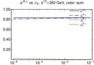
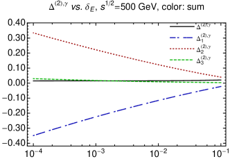
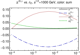
Figure 1: Dependence of separate contributions to $\Delta^{(2),\gamma}$ with full colors on the cut-off for different collision energies.

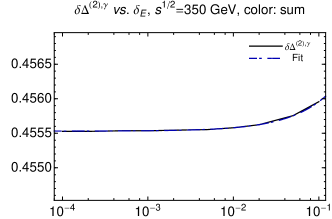
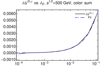
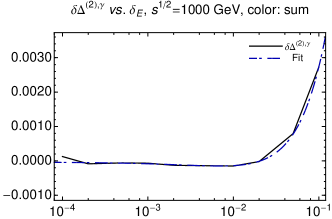
Figure 2: Dependence of $\delta\Delta^{(2),\gamma}$ with full colors on the cut-off and the fitted curves for different collision energies.

Fig. 3 shows detailed comparison of our numerical results with the threshold hep-ph/9712222 ; hep-ph/9712302 and high-energy expansion results hep-ph/9710413 ; hep-ph/9704222 in the threshold, transition, and high-energy region for a fixed $\delta_{E}=2\times 10^{-4}$. It can be seen that our full results works well in the entire energy region, i.e., approaching the threshold results for lower energies and the high-energy expansions on another end, while the other twos are not. However, one may notice the differences between the high-energy expansion results and ours for $\sqrt{s}>1200$ GeV. Though the differences are only at a level of a few times $10^{-4}$. The comparison are also shown in terms of $R^{(2)}$ in Figs. 4-5 as functions of $r$ for different color contributions. From Fig. 5 we can see more clearly the differences in regions of $r<0.3$, especially for the Abelian and heavy-fermionic contributions. Most of these differences are attributed to the inclusion of double-real corrections with four top quark final state in hep-ph/9710413 ; hep-ph/9704222 , which are not included in our calculations by default. We calculate those contributions to $R^{(2)}$ separately as shown in Fig. 6, which are only non-negligible for $r<0.3$. They are positive for the Abelian and heavy-fermionic parts of $R^{(2)}$ and negative for the non-Abelian part. These four top contributions have been checked against hep-ph/9705295 and found in very good agreement. Another reason is because we choose a finite value of $\delta_{E}=2\times 10^{-4}$, for which the $f_{1}$ and $f_{2}$ terms add up to about $10^{-4}$ for Abelian and non-Abelian parts with $\sqrt{s}=2000$ GeV .

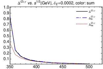
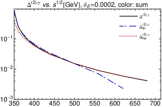
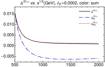
Figure 3: Comparison of $\Delta^{(2),\gamma}$ with the threshold results $\Delta^{(2),\gamma}_{th}$ and high-energy expansion results $\Delta^{(2),\gamma}_{he}$ in the threshold, transition, and high-energy region.

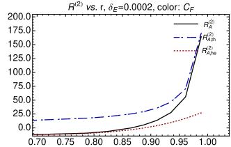
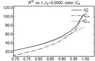
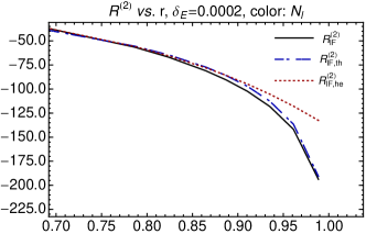
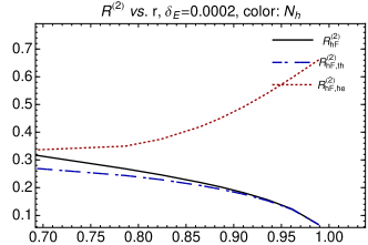
Figure 4: Comparison of different color contributions of $R^{(2)}$ with the threshold results $R^{(2)}_{th}$ and high-energy expansion results $R^{(2)}_{he}$ in the threshold region.

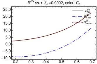
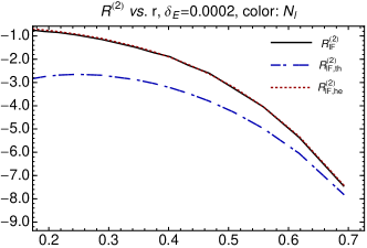
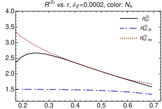
Figure 5: Comparison of different color contributions of $R^{(2)}$ with the threshold results $R^{(2)}_{th}$ and high-energy expansion results $R^{(2)}_{he}$ in the high-energy region.

Figure 6: Contributions to $R^{(2)}$ with different color structure from double-real corrections of four top quark final states.

We further show reduction of the scale variations by including the $\mathcal{O}(\alpha^{2}_{s})$ corrections in Fig. 7. We vary the renormalization scale $\mu_{r}$ around the nominal choice $\mu_{r}=\sqrt{s}$ by a factor of 10 downward and 4 upward. The scale dependence have been reduced significantly for $\sqrt{s}=$ 500 and 1000 GeV, e.g., from 6% at the NLO to 1% at the NNLO for a collision energy of 500 GeV. The NNLO results still show a large scale dependence near production threshold due to the large corrections and require resummations for further improvements.

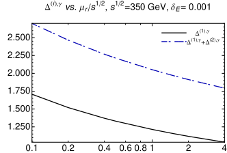
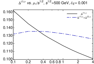
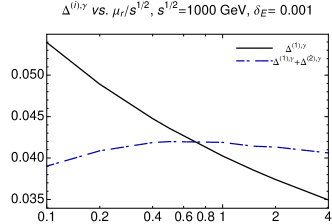
Figure 7: Scale dependence of $\Delta^{(1),\gamma}$ and $\Delta^{(1),\gamma}+\Delta^{(2),\gamma}$ for different collision energies.

3.2 Differential distributions

We can calculate fully differential distributions up to NNLO in QCD based on the phase-space slicing method. At LO, there is only one non-trivial kinematic variable, which we can choose either as cosine of the scattering angle between the final-state top quark and the initial-state electron $\cos\theta_{t}$, or transverse momentum of the top quark with respect to the beam $p_{T,t}$. Similar as the inclusive cross section, we can define the $\mathcal{O}(\alpha_{s})$ and $\mathcal{O}(\alpha^{2}_{s})$ corrections for each kinematic bin, $\Delta^{(1),\gamma}_{bin}$ and $\Delta^{(2),\gamma}_{bin}$, in analogy to Eq. (45). The results are shown in Fig. 8 for $\cos\theta_{t}$ and 9 for $p_{T,t}$ distributions with collision energies of 350, 500, and 1000 GeV. For each of them we plot the $\mathcal{O}(\alpha^{2}_{s})$ corrections with two different $\delta_{E}$ choices, $10^{-3}$ and $5\times 10^{-4}$. By comparing those two results we can see very good stabilities of the $\mathcal{O}(\alpha^{2}_{s})$ distributions for $\delta_{E}$ small enough $\sim$ a few $10^{-4}$, similar as the inclusive cross sections.

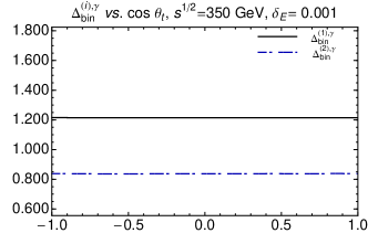
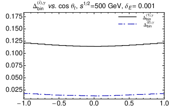
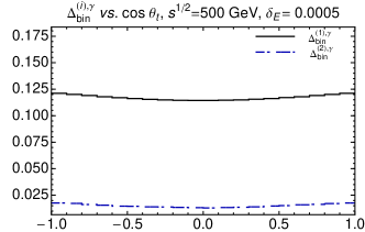
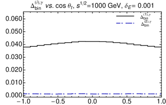
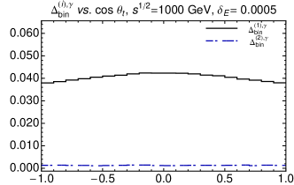
Figure 8: $\mathcal{O}(\alpha_{s})$ and $\mathcal{O}(\alpha_{s}^{2})$ corrections in different $\cos\theta_{t}$ bins, $\Delta^{(1),\gamma}_{bin}$ and $\Delta^{(2),\gamma}_{bin}$ for different collision energies and different $\delta_{E}$ choices.

As can be seen from Fig. 8, both the $\mathcal{O}(\alpha_{s})$ and $\mathcal{O}(\alpha^{2}_{s})$ corrections are flat for $\sqrt{s}=350$ GeV where they are dominated by virtual corrections. The $\cos\theta_{t}$ distribution is symmetric in forward and backward region for pure photon contributions. For $\sqrt{s}=500$ GeV, the $\mathcal{O}(\alpha^{2}_{s})$ corrections are slightly larger in region of $|\cos\theta_{t}|\sim 1$ than central region, and are about 13% of the $\mathcal{O}(\alpha_{s})$ corrections in size. The $\mathcal{O}(\alpha^{2}_{s})$ corrections for $\cos\theta_{t}$ distribution are totally negligible comparing to the $\mathcal{O}(\alpha_{s})$ ones for $\sqrt{s}=1000$ GeV.

The transverse momentum distributions in Fig. 9 show a different feature comparing to the angular distribution since they are also affected by the energy spectrum of the top quark. The real corrections pull the energy spectrum to the lower end and thus the $p_{T,t}$ distribution as well. As shown in Fig. 9, both the $\mathcal{O}(\alpha_{s})$ and $\mathcal{O}(\alpha^{2}_{s})$ corrections start as positive in low $p_{T}$ and then decrease to negative values near the kinematic limits. The $\mathcal{O}(\alpha^{2}_{s})$ corrections show a relatively larger impact in the $p_{T,t}$ distribution.

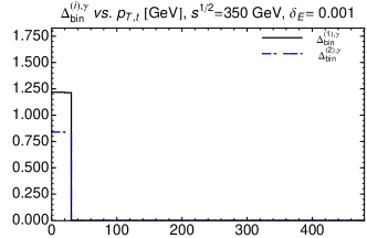
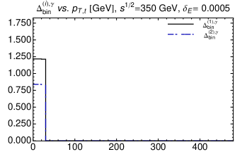
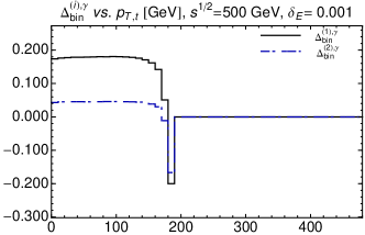
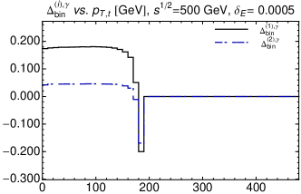
Figure 9: NLO and NNLO corrections in different $p_{T,t}$ bins, $\Delta^{(1),\gamma}_{bin}$ and $\Delta^{(2),\gamma}_{bin}$, for different collision energies and different $\delta_{E}$ choices.

Besides, we can also investigate distributions like, $\Delta\phi_{t\bar{t}}$, difference of azimuthal angles of top and antitop quark, and their invariant mass, $m_{t\bar{t}}$. Since they are both a delta function at the LO, our $\mathcal{O}(\alpha^{2}_{s})$ corrections are effectively NLO for those observables. We plot the LO distributions together with the $\mathcal{O}(\alpha_{s})$ and $\mathcal{O}(\alpha^{2}_{s})$ corrections in Fig. 10. The corrections have been rescaled for comparison. For bins with vanishing cross sections at the LO, we have compared our $\mathcal{O}(\alpha_{s})$ and $\mathcal{O}(\alpha^{2}_{s})$ corrections with the calculations of $Q\bar{Q}+jet$ production up to NLO in hep-ph/9705295 and found very good agreement.

Figure 10: Differential distribution, $d\sigma/dm_{t\bar{t}}$ on left, $d\sigma/d\phi_{t\bar{t}}$ on right, at the LO, $\mathcal{O}(\alpha_{s})$ (multiplied by 4), and $\mathcal{O}(\alpha_{s}^{2})$ (multiplied by 10).

4 Conclusion

To conclude, we have presented a fully differential NNLO QCD calculation for the photon exchange contributions to electroweak top quark pairs production at $e^{+}e^{-}$ colliders. Our calculations are based on a NNLO generalization of the phase-space slicing method. Similar methods were introduced some time ago to compute the $N_{l}$-dependent contributions to the total cross section hep-ph/9505262 ; hep-ph/9707496 . To the best of our knowledge, the results presented in this paper for the rest of the color structures are new. Let us emphasize that we present various differential distributions as well at NNLO for the first time. Whenever possible, we have compared our results to existing analytical calculations. We find complete agreement with the known results, both in the threshold hep-ph/9712222 ; hep-ph/9712302 ; hep-ph/9801397 ; hep-ph/0001286 and in the high-energy regimes Gorishnii:1986pz ; PHLTA.B248.359 ; hep-ph/9406299 ; hep-ph/9710413 ; hep-ph/9704222 . Although their calculation was beyond the scope of this work, the $Z$ exchange contributions can be straightforwardly derived using the phase-space slicing technique discussed in this paper. The $Z$ exchange contributions are of fundamental phenomenological importance and will be treated in a future publication.

Inspired by the successful application of $q_{T}$ subtraction method of Catani and Grazzini hep-ph/0703012 , recently there has been some interest and progress in applying the phase-space slicing method to NNLO QCD calculations. For instance, top quark decay 1210.2808 , Drell-Yan production 1405.3607 , and Higgs production 1407.3773 have all been studied in schemes very similar to the one described in this work. This paper demonstrates that phase-space slicing can also be used to calculate top quark production processes, albeit at $e^{+}e^{-}$ colliders. Our calculation shows that fully differential NNLO corrections in $e^{+}e^{-}$ annihilation are not much harder to obtain than typical NLO corrections to QCD processes once a good IR-safe observable has been defined and the corresponding hard and soft functions are known. In future work, it would be interesting to apply the phase-space slicing method to other NNLO QCD calculations relevant to the physics of future linear colliders and to generalize the method to allow for the treatment of parton-initiated processes.

- (1) S. Schael et al. [ALEPH and DELPHI and L3 and OPAL and SLD and LEP Electroweak Working Group and SLD Electroweak Group and SLD Heavy Flavour Group Collaborations], Phys. Rept. 427, 257 (2006) [hep-ex/0509008].
- (2) E. Devetak, A. Nomerotski and M. Peskin, Phys. Rev. D 84, 034029 (2011) [arXiv:1005.1756 [hep-ex]].
- (3) J. Jersak, E. Laermann and P. M. Zerwas, Phys. Rev. D 25, 1218 (1982) [Erratum-ibid. D 36, 310 (1987)].
- (4) W. Beenakker, S. C. van der Marck and W. Hollik, Nucl. Phys. B 365, 24 (1991).
- (5) C. R. Schmidt, Phys. Rev. D 54, 3250 (1996) [hep-ph/9504434].
- (6) J. Kodaira, T. Nasuno and S. J. Parke, Phys. Rev. D 59, 014023 (1998) [hep-ph/9807209].
- (7) H. X. Liu, C. S. Li and Z. J. Xiao, Phys. Lett. B 458, 393 (1999) [hep-ph/9901205].
- (8) A. Czarnecki and K. Melnikov, Phys. Rev. Lett. 80, 2531 (1998) [hep-ph/9712222].
- (9) M. Beneke, A. Signer and V. A. Smirnov, Phys. Rev. Lett. 80, 2535 (1998) [hep-ph/9712302].
- (10) A. H. Hoang and T. Teubner, Phys. Rev. D 58, 114023 (1998) [hep-ph/9801397].
- (11) A. H. Hoang, M. Beneke, K. Melnikov, T. Nagano, A. Ota, A. A. Penin, A. A. Pivovarov and A. Signer et al., Eur. Phys. J. direct C 2, 1 (2000) [hep-ph/0001286].
- (12) S. J. Brodsky, A. H. Hoang, J. H. Kuhn and T. Teubner, Phys. Lett. B 359, 355 (1995) [hep-ph/9508274].
- (13) S. G. Gorishnii, A. L. Kataev and S. A. Larin, Nuovo Cim. A 92, 119 (1986).
- (14) K. G. Chetyrkin and J. H. Kuhn, Phys. Lett. B 248, 359 (1990).
- (15) K. G. Chetyrkin and J. H. Kuhn, Nucl. Phys. B 432, 337 (1994) [hep-ph/9406299].
- (16) R. Harlander and M. Steinhauser, Eur. Phys. J. C 2, 151 (1998) [hep-ph/9710413].
- (17) K. G. Chetyrkin, R. Harlander, J. H. Kuhn and M. Steinhauser, Nucl. Phys. B 503, 339 (1997) [hep-ph/9704222].
- (18) G. Altarelli and B. Lampe, Nucl. Phys. B 391, 3 (1993).
- (19) V. Ravindran and W. L. van Neerven, Phys. Lett. B 445, 214 (1998) [hep-ph/9809411].
- (20) S. Catani and M. H. Seymour, JHEP 9907, 023 (1999) [hep-ph/9905424].
- (21) M. Beneke, Y. Kiyo and K. Schuller, arXiv:1312.4791 [hep-ph].
- (22) P. Marquard, J. H. Piclum, D. Seidel and M. Steinhauser, Phys. Rev. D 89, 034027 (2014) [arXiv:1401.3004 [hep-ph]].
- (23) M. Beneke, Y. Kiyo, P. Marquard, A. Penin, J. Piclum, D. Seidel and M. Steinhauser, Phys. Rev. Lett. 112, 151801 (2014) [arXiv:1401.3005 [hep-ph]].
- (24) G. Rodrigo, A. Santamaria and M. S. Bilenky, Phys. Rev. Lett. 79, 193 (1997) [hep-ph/9703358].
- (25) P. Nason and C. Oleari, Phys. Lett. B 407, 57 (1997) [hep-ph/9705295].
- (26) A. Brandenburg and P. Uwer, Nucl. Phys. B 515, 279 (1998) [hep-ph/9708350].
- (27) P. Nason and C. Oleari, Nucl. Phys. B 521, 237 (1998) [hep-ph/9709360].
- (28) G. Rodrigo, M. S. Bilenky and A. Santamaria, Nucl. Phys. B 554, 257 (1999) [hep-ph/9905276].
- (29) W. Bernreuther, R. Bonciani, T. Gehrmann, R. Heinesch, T. Leineweber, P. Mastrolia and E. Remiddi, Nucl. Phys. B 706, 245 (2005) [hep-ph/0406046].
- (30) W. Bernreuther, R. Bonciani, T. Gehrmann, R. Heinesch, T. Leineweber, P. Mastrolia and E. Remiddi, Nucl. Phys. B 712, 229 (2005) [hep-ph/0412259].
- (31) W. Bernreuther, R. Bonciani, T. Gehrmann, R. Heinesch, T. Leineweber and E. Remiddi, Nucl. Phys. B 723, 91 (2005) [hep-ph/0504190].
- (32) J. Gluza, A. Mitov, S. Moch and T. Riemann, JHEP 0907, 001 (2009) [arXiv:0905.1137 [hep-ph]].
- (33) K. Fabricius, I. Schmitt, G. Kramer and G. Schierholz, Z. Phys. C 11 (1981) 315.
- (34) G. Kramer and B. Lampe, Fortsch. Phys. 37, 161 (1989).
- (35) H. Baer, J. Ohnemus and J. F. Owens, Phys. Rev. D 40, 2844 (1989).
- (36) W. T. Giele and E. W. N. Glover, Phys. Rev. D 46, 1980 (1992).
- (37) W. T. Giele, E. W. N. Glover and D. A. Kosower, Nucl. Phys. B 403, 633 (1993) [hep-ph/9302225].
- (38) B. W. Harris and J. F. Owens, Phys. Rev. D 65, 094032 (2002) [hep-ph/0102128].
- (39) S. Keller and E. Laenen, Phys. Rev. D 59, 114004 (1999) [hep-ph/9812415].
- (40) R. K. Ellis, D. A. Ross and A. E. Terrano, Nucl. Phys. B 178, 421 (1981).
- (41) M. L. Mangano, P. Nason and G. Ridolfi, Nucl. Phys. B 373, 295 (1992).
- (42) Z. Kunszt and D. E. Soper, Phys. Rev. D 46, 192 (1992).
- (43) S. Frixione, Z. Kunszt and A. Signer, Nucl. Phys. B 467, 399 (1996) [hep-ph/9512328].
- (44) S. Catani and M. H. Seymour, Nucl. Phys. B 485, 291 (1997) [Erratum-ibid. B 510, 503 (1998)] [hep-ph/9605323].
- (45) S. Catani, S. Dittmaier, M. H. Seymour and Z. Trocsanyi, Nucl. Phys. B 627, 189 (2002) [hep-ph/0201036].
- (46) A. Gehrmann-De Ridder, T. Gehrmann, E. W. N. Glover and J. Pires, Phys. Rev. Lett. 110, no. 16, 162003 (2013) [arXiv:1301.7310 [hep-ph]].
- (47) J. Currie, A. Gehrmann-De Ridder, E. W. N. Glover and J. Pires, JHEP 1401, 110 (2014) [arXiv:1310.3993 [hep-ph]].
- (48) Z. Bern, L. J. Dixon and D. A. Kosower, JHEP 0001, 027 (2000) [hep-ph/0001001].
- (49) V. A. Smirnov, Phys. Lett. B 460, 397 (1999) [hep-ph/9905323].
- (50) J. B. Tausk, Phys. Lett. B 469, 225 (1999) [hep-ph/9909506].
- (51) C. Anastasiou, T. Gehrmann, C. Oleari, E. Remiddi and J. B. Tausk, Nucl. Phys. B 580, 577 (2000) [hep-ph/0003261].
- (52) C. Anastasiou, E. W. N. Glover, C. Oleari and M. E. Tejeda-Yeomans, Nucl. Phys. B 601, 318 (2001) [hep-ph/0010212].
- (53) C. Anastasiou, E. W. N. Glover, C. Oleari and M. E. Tejeda-Yeomans, Nucl. Phys. B 601, 341 (2001) [hep-ph/0011094].
- (54) C. Anastasiou, E. W. N. Glover, C. Oleari and M. E. Tejeda-Yeomans, Phys. Lett. B 506, 59 (2001) [hep-ph/0012007].
- (55) C. Anastasiou, E. W. N. Glover, C. Oleari and M. E. Tejeda-Yeomans, Nucl. Phys. B 605, 486 (2001) [hep-ph/0101304].
- (56) E. W. N. Glover, C. Oleari and M. E. Tejeda-Yeomans, Nucl. Phys. B 605, 467 (2001) [hep-ph/0102201].
- (57) E. W. N. Glover and M. E. Tejeda-Yeomans, JHEP 0105, 010 (2001) [hep-ph/0104178].
- (58) T. Binoth and G. Heinrich, Nucl. Phys. B 585, 741 (2000) [hep-ph/0004013].
- (59) S. Weinzierl, JHEP 0303, 062 (2003) [hep-ph/0302180].
- (60) S. Weinzierl, JHEP 0307, 052 (2003) [hep-ph/0306248].
- (61) C. Anastasiou, K. Melnikov and F. Petriello, Phys. Rev. D 69, 076010 (2004) [hep-ph/0311311].
- (62) T. Binoth and G. Heinrich, Nucl. Phys. B 693, 134 (2004) [hep-ph/0402265].
- (63) C. Anastasiou, K. Melnikov and F. Petriello, Phys. Rev. Lett. 93, 032002 (2004) [hep-ph/0402280].
- (64) A. Gehrmann-De Ridder, T. Gehrmann and E. W. N. Glover, Nucl. Phys. B 691, 195 (2004) [hep-ph/0403057].
- (65) C. Anastasiou, K. Melnikov and F. Petriello, Phys. Rev. Lett. 93, 262002 (2004) [hep-ph/0409088].
- (66) S. Frixione and M. Grazzini, JHEP 0506, 010 (2005) [hep-ph/0411399].
- (67) G. Somogyi, Z. Trocsanyi and V. Del Duca, JHEP 0506, 024 (2005) [hep-ph/0502226].
- (68) A. Gehrmann-De Ridder, T. Gehrmann and E. W. N. Glover, JHEP 0509, 056 (2005) [hep-ph/0505111].
- (69) K. Melnikov and F. Petriello, Phys. Rev. Lett. 96, 231803 (2006) [hep-ph/0603182].
- (70) G. Somogyi, Z. Trocsanyi and V. Del Duca, JHEP 0701, 070 (2007) [hep-ph/0609042].
- (71) G. Somogyi and Z. Trocsanyi, JHEP 0701, 052 (2007) [hep-ph/0609043].
- (72) S. Catani and M. Grazzini, Phys. Rev. Lett. 98, 222002 (2007) [hep-ph/0703012].
- (73) A. Gehrmann-De Ridder, T. Gehrmann, E. W. N. Glover and G. Heinrich, JHEP 0711, 058 (2007) [arXiv:0710.0346 [hep-ph]].
- (74) A. Gehrmann-De Ridder, T. Gehrmann, E. W. N. Glover and G. Heinrich, Phys. Rev. Lett. 100, 172001 (2008) [arXiv:0802.0813 [hep-ph]].
- (75) G. Somogyi and Z. Trocsanyi, JHEP 0808, 042 (2008) [arXiv:0807.0509 [hep-ph]].
- (76) S. Weinzierl, Phys. Rev. Lett. 101, 162001 (2008) [arXiv:0807.3241 [hep-ph]].
- (77) K. Melnikov, Phys. Lett. B 666, 336 (2008) [arXiv:0803.0951 [hep-ph]].
- (78) U. Aglietti, V. Del Duca, C. Duhr, G. Somogyi and Z. Trocsanyi, JHEP 0809, 107 (2008) [arXiv:0807.0514 [hep-ph]].
- (79) S. Catani, L. Cieri, G. Ferrera, D. de Florian and M. Grazzini, Phys. Rev. Lett. 103, 082001 (2009) [arXiv:0903.2120 [hep-ph]].
- (80) S. Weinzierl, JHEP 0907, 009 (2009) [arXiv:0904.1145 [hep-ph]].
- (81) P. Bolzoni, S. O. Moch, G. Somogyi and Z. Trocsanyi, JHEP 0908, 079 (2009) [arXiv:0905.4390 [hep-ph]].
- (82) A. Daleo, A. Gehrmann-De Ridder, T. Gehrmann and G. Luisoni, JHEP 1001, 118 (2010) [arXiv:0912.0374 [hep-ph]].
- (83) E. W. Nigel Glover and J. Pires, JHEP 1006, 096 (2010) [arXiv:1003.2824 [hep-ph]].
- (84) S. Biswas and K. Melnikov, JHEP 1002, 089 (2010) [arXiv:0911.4142 [hep-ph]].
- (85) P. Bolzoni, F. Maltoni, S. O. Moch and M. Zaro, Phys. Rev. Lett. 105, 011801 (2010) [arXiv:1003.4451 [hep-ph]].
- (86) M. Czakon, Phys. Lett. B 693, 259 (2010) [arXiv:1005.0274 [hep-ph]].
- (87) P. Bolzoni, G. Somogyi and Z. Trocsanyi, JHEP 1101, 059 (2011) [arXiv:1011.1909 [hep-ph]].
- (88) R. Boughezal, A. Gehrmann-De Ridder and M. Ritzmann, JHEP 1102, 098 (2011) [arXiv:1011.6631 [hep-ph]].
- (89) M. Czakon, Nucl. Phys. B 849, 250 (2011) [arXiv:1101.0642 [hep-ph]].
- (90) W. Bernreuther, C. Bogner and O. Dekkers, JHEP 1106, 032 (2011) [arXiv:1105.0530 [hep-ph]].
- (91) T. Gehrmann and P. F. Monni, JHEP 1112, 049 (2011) [arXiv:1107.4037 [hep-ph]].
- (92) G. Ferrera, M. Grazzini and F. Tramontano, Phys. Rev. Lett. 107, 152003 (2011) [arXiv:1107.1164 [hep-ph]].
- (93) C. Anastasiou, F. Herzog and A. Lazopoulos, JHEP 1203, 035 (2012) [arXiv:1110.2368 [hep-ph]].
- (94) S. Catani, L. Cieri, D. de Florian, G. Ferrera and M. Grazzini, Phys. Rev. Lett. 108, 072001 (2012) [arXiv:1110.2375 [hep-ph]].
- (95) G. Abelof and A. Gehrmann-De Ridder, JHEP 1204, 076 (2012) [arXiv:1112.4736 [hep-ph]].
- (96) P. Bärnreuther, M. Czakon and A. Mitov, Phys. Rev. Lett. 109, 132001 (2012) [arXiv:1204.5201 [hep-ph]].
- (97) A. Gehrmann-De Ridder, T. Gehrmann and M. Ritzmann, JHEP 1210, 047 (2012) [arXiv:1207.5779 [hep-ph]].
- (98) G. Abelof and A. Gehrmann-De Ridder, JHEP 1211, 074 (2012) [arXiv:1207.6546 [hep-ph]].
- (99) J. Gao, C. S. Li and H. X. Zhu, Phys. Rev. Lett. 110, 042001 (2013) [arXiv:1210.2808 [hep-ph]].
- (100) G. Abelof, O. Dekkers and A. Gehrmann-De Ridder, JHEP 1212, 107 (2012) [arXiv:1210.5059 [hep-ph]].
- (101) J. Currie, E. W. N. Glover and S. Wells, JHEP 1304, 066 (2013) [arXiv:1301.4693 [hep-ph]].
- (102) M. Brucherseifer, F. Caola and K. Melnikov, JHEP 1304, 059 (2013) [arXiv:1301.7133 [hep-ph]].
- (103) R. Boughezal, F. Caola, K. Melnikov, F. Petriello and M. Schulze, JHEP 1306, 072 (2013) [arXiv:1302.6216 [hep-ph]].
- (104) M. Czakon, P. Fiedler and A. Mitov, Phys. Rev. Lett. 110, no. 25, 252004 (2013) [arXiv:1303.6254 [hep-ph]].
- (105) W. Bernreuther, C. Bogner and O. Dekkers, JHEP 1310, 161 (2013) [arXiv:1309.6887 [hep-ph]].
- (106) M. Grazzini, S. Kallweit, D. Rathlev and A. Torre, Phys. Lett. B 731, 204 (2014) [arXiv:1309.7000 [hep-ph]].
- (107) L. Liu-Sheng, Z. Ren-You, M. Wen-Gan, G. Lei, L. Wei-Hua and L. Xiao-Zhou, Phys. Rev. D 89, 073001 (2014) [arXiv:1401.7754 [hep-ph]].
- (108) G. Abelof, A. Gehrmann-De Ridder, P. Maierhofer and S. Pozzorini, arXiv:1404.6493 [hep-ph].
- (109) M. Brucherseifer, F. Caola and K. Melnikov, arXiv:1404.7116 [hep-ph].
- (110) F. Cascioli, T. Gehrmann, M. Grazzini, S. Kallweit, P. Maierhöfer, A. von Manteuffel, S. Pozzorini and D. Rathlev et al., arXiv:1405.2219 [hep-ph].
- (111) C. Anastasiou, J. Cancino, F. Chavez, C. Duhr, A. Lazopoulos, B. Mistlberger and R. Mueller, arXiv:1408.4546 [hep-ph].
- (112) A. H. Hoang, M. Jezabek, J. H. Kuhn and T. Teubner, Phys. Lett. B 338, 330 (1994) [hep-ph/9407338].
- (113) K. G. Chetyrkin, A. H. Hoang, J. H. Kuhn, M. Steinhauser and T. Teubner, In *Annecy/Assergi/Hamburg 1995, e+ e- collisions at TeV energies, pt. B* 29-32 [hep-ph/9605311].
- (114) A. H. Hoang, J. H. Kuhn and T. Teubner, Nucl. Phys. B 452, 173 (1995) [hep-ph/9505262].
- (115) A. H. Hoang and T. Teubner, Nucl. Phys. B 519, 285 (1998) [hep-ph/9707496].
- (116) C. W. Bauer, D. Pirjol and I. W. Stewart, Phys. Rev. D 65, 054022 (2002) [hep-ph/0109045].
- (117) T. Becher, M. Neubert and B. D. Pecjak, JHEP 0701, 076 (2007) [hep-ph/0607228].
- (118) S. A. Larin, T. van Ritbergen and J. A. M. Vermaseren, Nucl. Phys. B 438, 278 (1995) [hep-ph/9411260].
- (119) K. G. Chetyrkin, B. A. Kniehl and M. Steinhauser, Phys. Rev. Lett. 79, 2184 (1997) [hep-ph/9706430].
- (120) K. G. Chetyrkin, B. A. Kniehl and M. Steinhauser, Nucl. Phys. B 510, 61 (1998) [hep-ph/9708255].
- (121) K. G. Chetyrkin, J. H. Kuhn and M. Steinhauser, Comput. Phys. Commun. 133, 43 (2000) [hep-ph/0004189].
- (122) A. Mitov and S. Moch, JHEP 0705, 001 (2007) [hep-ph/0612149].
- (123) E. Remiddi and J. A. M. Vermaseren, Int. J. Mod. Phys. A 15, 725 (2000) [hep-ph/9905237].
- (124) T. Gehrmann and E. Remiddi, Comput. Phys. Commun. 141, 296 (2001) [hep-ph/0107173].
- (125) A. von Manteuffel, R. M. Schabinger, H. X. Zhu, “The two-loop soft function for heavy quark pair production at future linear colliders”, in press.
- (126) G. P. Korchemsky and A. V. Radyushkin, Nucl. Phys. B 283, 342 (1987).
- (127) N. Kidonakis, Phys. Rev. Lett. 102, 232003 (2009) [arXiv:0903.2561 [hep-ph]].
- (128) T. Becher and M. Neubert, Phys. Rev. D 79, 125004 (2009) [Erratum-ibid. D 80, 109901 (2009)] [arXiv:0904.1021 [hep-ph]].
- (129) S. Catani, S. Dittmaier, M. H. Seymour and Z. Trocsanyi, Nucl. Phys. B 627, 189 (2002) [hep-ph/0201036].
- (130) G. Cullen, H. van Deurzen, N. Greiner, G. Heinrich, G. Luisoni, P. Mastrolia, E. Mirabella and G. Ossola et al., arXiv:1404.7096 [hep-ph].
- (131) P. Mastrolia, E. Mirabella and T. Peraro, JHEP 1206, 095 (2012) [Erratum-ibid. 1211, 128 (2012)] [arXiv:1203.0291 [hep-ph]].
- (132) T. Peraro, Comput. Phys. Commun. 185, 2771 (2014) [arXiv:1403.1229 [hep-ph]].
- (133) A. van Hameren, C. G. Papadopoulos and R. Pittau, JHEP 0909, 106 (2009) [arXiv:0903.4665 [hep-ph]].
- (134) A. van Hameren, Comput. Phys. Commun. 182, 2427 (2011) [arXiv:1007.4716 [hep-ph]].
- (135) E. Laenen, L. Magnea, G. Stavenga and C. D. White, Nucl. Phys. Proc. Suppl. 205-206, 260 (2010) [arXiv:1007.0624 [hep-ph]].
- (136) E. Laenen, L. Magnea, G. Stavenga and C. D. White, JHEP 1101, 141 (2011) [arXiv:1010.1860 [hep-ph]].
- (137) A. Denner and T. Sack, Nucl. Phys. B 358, 46 (1991).
- (138) J. Beringer et al. [Particle Data Group Collaboration], Phys. Rev. D 86, 010001 (2012).
- (139) S. Höche, Y. Li and S. Prestel, arXiv:1405.3607 [hep-ph].
- (140) S. Höche, Y. Li and S. Prestel, arXiv:1407.3773 [hep-ph].