Next Generation Strong Lensing Time Delay Estimation with Gaussian Processes

Abstract

Strong gravitational lensing forms multiple, time delayed images of cosmological sources, with the “focal length” of the lens serving as a cosmological distance probe. Robust estimation of the time delay distance can tightly constrain the Hubble constant as well as the matter density and dark energy. Current and next generation surveys will find hundreds to thousands of lensed systems but accurate time delay estimation from noisy, gappy lightcurves is potentially a limiting systematic. Using a large sample of blinded lightcurves from the Strong Lens Time Delay Challenge we develop and demonstrate a Gaussian Process crosscorrelation technique that delivers an average bias within 0.1% depending on the sampling, necessary for subpercent Hubble constant determination. The fits are accurate (80% of them within 1 day) for delays from 5–100 days and robust against cadence variations shorter than 6 days. We study the effects of survey characteristics such as cadence, season, and campaign length, and derive requirements for time delay cosmology: in order not to bias the cosmology determination by $0.5\sigma$, the mean time delay fit accuracy must be better than 0.2%.

I Introduction

Strong lensing time delay cosmography is a promising probe that has developed rapidly in the last few years. In 2012, two strong lens time delay distances, combined with then-current cosmic microwave background (CMB) data, demonstrated as much constraining power on dark energy density and spatial curvature as then-current baryon acoustic oscillation distance data suyu12 . In 2013, a single time delay distance combined with CMB data determined the Hubble constant to 7% in a dark energy model (wCDM), while CMB data alone nearly filled its prior suyu13 . A Hubble Space Telescope program to more than double the number of precisely modeled time delay lens systems is now underway holicow .

The two main cosmological advantages that strong lensing time delay distances bring are: 1) sensitivity to the Hubble constant $H_{0}$, since the time delay distance is a dimensionful quantity, measured from an observable time delay, and 2) excellent complementarity with other probes when constraining dark energy properties such as time varying equation of state lin04 ; lin11 . On top of this, the time delay distance is a geometric quantity, independent of the details of the growth of structure or galaxy bias. For further discussion of time delay distances as a cosmological probe, see snowsl .

Currently, the main observational challenges for the use of time delay distances are finding a large sample of lensed systems, photometrically monitoring them every few days over a period of several years, and following them up spectroscopically to establish redshifts and with high resolution imaging to model the lens galaxy mass distribution. The first issues will become moot with the current and next generation of wide field, time domain surveys such as Dark Energy Survey (DES; des ) and the Large Synoptic Survey Telescope (LSST; lsst ). Likewise spectroscopic redshifts can be obtained efficiently with new multiobject spectrographs such as DESI desi and PFS pfs . High resolution imaging may become easier as the HST time becomes less oversubscribed, the more powerful JWST is in operation, and ground based adaptive optics develops further.

The major analysis challenges are the robust estimation of the actual time delays between images, derived from noisy, gappy lightcurves, and the modeling of the lens mass distribution and the mass along the line of sight. We concentrate on the first of these, and indeed it is the focus of a series of Strong Lens Data Challenges tdc0 ; tdc1 . The mass modeling is also developing rapidly oguri07 ; suyu09 ; suyu10 ; suyu12 ; collett ; greene and all three sources of uncertainty must be reduced together to obtain time delay distances with 5% or better precision and subpercent accuracy.

In Sec. II we describe our application of the Gaussian Process statistical technique to time delay estimation. We review the Time Delay Challenge metrics in Sec. III and present our original blinded analysis. Section IV describes improvements to the statistical methodology and their results. We discuss cosmological requirements on accuracy to obtain next generation constraints on the Hubble constant and dark energy in Sec. V and conclude in Sec. VI.

II Gaussian Process Technique

We employ Gaussian Process (GP) regression to estimate the time delays between the multiple image lightcurves of a strongly lensed source. GP is commonly used as a robust and fairly model-independent technique for reconstructing an underlying function from noisy measurements. In GP regression, the underlying function is not parametrized but instead a complete set of possible curves is fitted to the data points. The curves are constructed from a mean function, describing the average behavior of the function, and a covariance kernel imposing a Gaussian correlation between the data points and serving to describe the fluctuation of those points around the mean function. The covariance function is characterized by a set of hyperparameters which control the amplitude and length of the correlation between the data points.

Our data here are the lightcurve magnitude measurements of multiple images of a source. (We should emphasize that here our focus is extracting accurate time delays, not modeling the intrinsic lightcurve of the source.) While the measurements are made on the same underlying intrinsic lightcurve, there is a time delay between each pair of the observed lightcurves, and that is what we want to determine. We quantify the time delays with a set of $\Delta t_{i}$ parameters and fit them to data together with the GP hyperparameters of our kernel function. As described in detail in GPpaper , the kernel function includes different terms: the GP kernel (as described above) that describes the intrinsic variability of the source (generally a quasar); a separate microlensing kernel that accounts for the (longer term) variations in magnitude due to microlensing (from substructure in the lensing galaxy and along the line of sight); and a nugget term, an additional constant variance in measurements that acts as a zero lag dispersion accounting for e.g. misestimated measurement noise or scatter due to the finite realization nature of the data.

To fit the parameters, we utilize the GP likelihood gpml :

$$2\ln\mathcal{L}(Y|\vec{\theta})=-Y^{T}K^{-1}Y-\ln|K|-N_{d}\,\ln 2\pi,$$ (1)

where $Y$ is the vector of magnitude data, with $N_{d}$ the total number of data points, $\vec{\theta}$ represents the fit parameters, e.g. time delays, and $|K|$ is the determinant of the kernel $K$, giving a complexity penalty.

For the mean function, we adopt a constant value in this analysis as a good choice that preserves the distribution of data points, and hence any distinct features in the intrinsic source lightcurve, a necessary element in recovering accurate time delay by matching the observed lightcurves. We have tested other mean functions, including smoothing techniques, and found they did not perform as well.

For the covariance, we adopt two kernels, a damped random walk (DRW), which is often used to model the intrinsic quasar/active galactic nucleus (AGN) light curve drw1 ; drw2 ; drw4 ,

$$k(t_{i},t_{j})=\sigma^{2}\,e^{-|t_{i}-t_{j}|/l}\ ,$$ (2)

and a Matern function with index $3/2$ commonly used in statistics gpml :

$$k(t_{i},t_{j})=\sigma^{2}\left(1+\frac{|t_{i}-t_{j}|\sqrt{3}}{l}\right)\,e^{-|t_{i}-t_{j}|\sqrt{3}/l}\ .$$ (3)

In the above $t_{i}$ and $t_{j}$ are measurement times, the hyperparameter $\sigma$ adjusts the amplitude of the kernel and $l$ functions as a correlation length.

We use Minuit minuit as the likelihood minimizer, and also independently validate our fits from a Monte Carlo analysis. The use of two kernels, two optimizers, and variations of priors allow us to crosscheck our results and determine their robustness. The GP code is parallel and optimized to handle a large number of systems autonomously in an efficient manner.

III Time Delay Challenge – Blind Results

The Strong Lens Time Delay Challenge (TDC) tdc0 ; tdc1 provided the opportunity for the first systematic study of the current capabilities of the community in measuring time delays through a set of several thousand simulated lightcurves. The goal has been to evaluate whether the available methods were able to achieve the criteria required for handling next generation data and provide a diagnostic tool for improvements, and also to investigate the impact of different observational and systematic factors on the results.

For the TDC simulated data tdcweb , an “Evil Team” generated LSST-like lightcurves, including noise and systematics, without revealing the process or true time delay, and released the blinded data. The intrinsic AGN light curves were constructed from a DRW stochastic process and then different observational, photometric and systematic noise components were implemented progressively tdc0 ; tdc1 . First, microlensing contributions were added based on a simulated star magnification map for LSST. The dominant statistical noise contribution, sky brightness, was then included through a Gaussian random noise. On top of that, additional flux errors were implemented in the form of three types of “evilness” contaminating some of the simulated systems.

The main challenge (TDC1) consists of five rungs to cover a range of different observational strategies, namely, monitoring cadence and its dispersion, individual season length, and full campaign length. The details are summarized in Table I of tdc1 .

The TDC proposed in advance the following criteria (metrics) to evaluate the performance of methods:

• Submitted fraction, $f$:

  $$f\equiv\frac{N_{\rm sub}}{N}\,$$ (4)

  the fraction of the total number of systems $N$ for which time delays were estimated.

• Goodness of fit:

  $$\chi^{2}=\frac{1}{fN}\sum_{i}\left(\frac{\widetilde{\Delta t}_{i}-\Delta t_{i}}{\sigma_{i}}\,\right)^{2}$$ (5)

  where $\Delta t_{i}$ is the true time delay value for system $i$, and $\widetilde{\Delta t}_{i}$ and $\sigma_{i}$ are the estimated time delay and its uncertainty.

• Accuracy (or bias):

  $$A=\frac{1}{fN}\sum_{i}\frac{\widetilde{\Delta t}_{i}-\Delta t_{i}}{|\Delta t_{i}|}\ .$$ (6)

  This metric is important for getting an unbiased estimation of time delay distances and propagates directly into accurate determination of cosmological parameters. We discuss the cosmological requirements in Sec. V; TDC1 had a goal of $A<0.2\%$ tdc0 for next generation surveys.

• Precision:

  $$P=\frac{1}{fN}\sum_{i}\frac{\sigma_{i}}{|\Delta t_{i}|}\,$$ (7)

  which quantifies the fractional uncertainty in the time delays.

To estimate the time delays, we first run our GP code on the TDC data and fit the model parameters using both kernels and both optimizers. We then pass or reject each system, based on the consistency of fits and their likelihoods, and then assign a final best fit time delay and uncertainty. Finally, we rank our systems and give them confidence classes based on a set of selection criteria, a combination of the degree of consistency of estimated time delays from different kernels/minimizers, likelihoods, and reduced $\chi^{2}$.

For TDC1, we produced six different samples, with the main three representing progressively inclusive fit confidence, e.g. gold, silver, bronze: Lannister, Targaryen, and Baratheon. In addition, we studied other selection criteria: a conservatively selected sample (Tully) and one with tighter error assignment (Stark). We also developed an outlier detection algorithm to identify and remove catastrophic outliers through imposing controlled priors, and also an analysis of the best fit parameters for the selected systems. The Freefolk sample was the result of such analysis. The details of the statistics for these samples can be found in tdc1 .

Our effort has been mainly focused on two aspects: developing an automated method that can handle the large number ($\sim 5000$) of future strong lens systems, fast and efficient with minimum human labor requirements; and optimizing for the accuracy of the fits as a critical metric for using strong lensing time delays as an unbiased, robust cosmological distance probe.

After the deadline for the submission of TDC results, we revisited our code to study alternate mean functions and realized that our original step to “prewhiten” the lightcurves had not been fully implemented as intended. We made this correction, keeping everything else the same, so now the magnitude shift hyperparameter only has to account for residual shifts. This resulted in a significant improvement in the performance of our method. For example, for our leading blind submission of Stark the average fit success fraction for the harder rungs 1-4 climbed from $f\approx 0.18$ to $f\approx 0.33$.

In the next section, we demonstrate that our results are accurate well below TDC requirements for the $A$ metric, and with reasonable precision ($P$), fraction ($f$) and goodness of fit ($\chi^{2}$).

IV Improvements to Time Delay Estimation

IV.1 Criteria

To this point, we have followed the code output blindly, and used the TDC framework criterion of $\chi_{i}^{2}<10$ to cut significant outliers. However, $\chi^{2}$ requires knowledge of the true time delay and so is not suitable for actual cosmological use. Therefore we now add some intelligence to the code, while maintaining uniform treatment for all systems.

The first condition considered is basic, and indeed could have been applied from the beginning if we had not wanted to test the fitting code in its purest form.

• Fit uncertainty: If the fit cannot deliver an uncertainty smaller than 4 days, i.e. $\sigma(\widetilde{\Delta t})<4$ days, then remove the system.

The second condition involves the accuracy. This is intended to clip extreme outliers. Since we will not know the true time delay, we cannot use it directly. However, we can identify outliers, not from the unknown true cosmology but from the cosmology derived from the global fit of all the time delay distances. That is, we compare a system against its peers. This statistical technique is frequently used in astrophysics, for example with supernova distance union . We take a very loose clipping, corresponding roughly to $4\sigma$:

• Global outlier: If the fit deviates by more than 20% from the truth, i.e. $|\widetilde{\Delta t}-\Delta t|/|\Delta t|>0.2$, then remove the system.

Since the global accuracy is good, and TDC1 provides no redshift information to derive a cosmology, we here take the global fit cosmology (and hence $\Delta t$ in this expression) to be the truth.

We emphasize that the crucial uncertainty $\sigma$ here is not that of the time delay estimation but of the entire time delay distance estimation, i.e. the cosmology estimation, including the uncertainties from other effects such as lens mass modeling and line of sight convergence. We take that the final uncertainty for the time delay distance of a system used for cosmology will be of order 5%; thus a 20% deviation in the time delay (translating into a 20% deviation in the distance, aside from contributions and covariances from the other quantities) will clearly stand out.

Those are the only two conditions we impose on our fits. We do not cut in $\chi^{2}$ or for time delays shorter than 10 days.

IV.2 Baseline results

Now we can examine the statistics for our improved set of fits, using the correct mean function treatment and the two conditions. Table 1 summarizes the evaluation metrics by rung.

Rung	$\qquad f\qquad$	$\qquad\chi^{2}\qquad$	$\qquad P\qquad$	$\qquad A\qquad$
0	0.48	1.07	0.0578	-0.0005
1	0.36	1.11	0.0617	-0.0010
2	0.31	1.14	0.0854	-0.0000
3	0.29	1.67	0.0688	-0.0019
4	0.36	1.92	0.0909	-0.0036
Avg	0.36	1.36	0.0717	-0.0014
Avg[3d]	0.36	1.22	0.0669	-0.0008

Table 1: Time delay estimation metrics are given for each rung of the challenge, and averaged over either all systems used or all systems with mean 3 day cadence (rungs 0-3).

On average about one-third of the systems can be used robustly for time delay cosmology. Given that LSST will find of order $10^{3-4}$ systems ogmar and we will be limited by followup observationally and by modeling uncertainties theoretically, such a fraction is quite acceptable. The fits achieve a mean accuracy, i.e. the bias with respect to the true time delay, of 0.14%; we address the cosmology requirements for this in the next section. The mean statistical precision is 7.2% and is seen to be improved by more data in the lightcurve, either a longer season (rung 0) or longer monitoring campaign (rung 1). It can also be reduced by the square root of the number of systems. We return to the precision in Sec. IV.4.

Apart from the effect of the number of lightcurve points, the major effect is that the six day cadence of rung 4 performs noticeably worse than the three day cadence rungs. The last row of Table 1, with only the three day cadence rungs, shows that the mean accuracy metric improves by almost a factor two, and that the precision for rung 4 is also significantly worse. Fixing the average cadence to three days, we see that rung 3 (with a $3\pm 1$ day cadence) has some advantage over rung 2 (fixed 3 day cadence), as its cadence variation allows some sampling on shorter time scales; we discuss this further below.

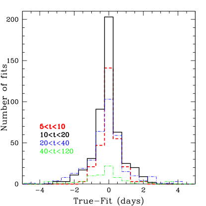
It is useful to look at the full distributions to find more subtle effects. First we consider whether there is any bias in estimation for time delays of different lengths. Figure 1 plots the histograms of the deviation of fit from truth for four ranges of time delays. The distributions are well peaked around zero and fairly symmetric. The longest time delays have the broadest distribution but fractionally are comparable, i.e. a 2 day offset in a 60 day time delay is like a 0.5 day offset in a 15 day time delay.

Figure 1: The distribution of the difference between the fitted time delay and the truth is plotted for four ranges of true time delay $t\equiv|\Delta t|$. No bias is apparent, and the distributions are well peaked.

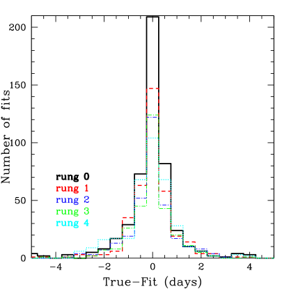
To study the effect of cadence and other survey characteristics, we investigate the distributions of results for different rungs of the challenge. Figure 2 demonstrates that for all rungs the time delay estimation has negligible bias and is highly peaked around zero deviation from the truth. For all rungs except rung 4, the ratio of the peak to the shoulders, i.e. the height of the zero bin vs the next bins, is $\sim 2.5$; however rung 4 with twice as long an average cadence gives a ratio of $\sim 1.5$, being more dispersed though still unbiased. This indicates that loosening the cadence from three days to six could impact the cosmology results. Over rungs 0-3, the fit offset is less than 0.5 (1.0) days for $\sim 62\%$ ($\sim 82\%$) of the systems; for rung 4 the numbers are 52% and 75% respectively.

Figure 2: The distribution of the difference between the fitted time delay and the truth is plotted for the five sets of survey characteristics corresponding to the Challenge rungs. No bias is apparent, and the distributions are well peaked, though the result of rung 4 with six day cadence is noticeably broader.

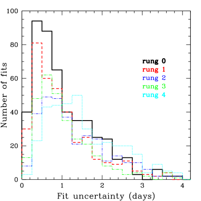
While our main focus is on accurate fits, we can also examine the impact of survey characteristics on statistical uncertainty of the fits. Figure 3 shows the distributions for the various rungs. The number of data points play a larger role here: rungs 0 and 1, with twice as many lightcurve points, have smaller uncertainties. There is also some difference between rungs 2 and 3, where rung 2 keeps a strict three day cadence while rung 3 varies it between two and four days. Rung 3 has a tighter distribution of fit uncertainties, hinting that such variation can be advantageous, with the occasional tighter cadence presumably allowing better crosscorrelations between the images at some points in the monitoring. Rung 4, with the six day cadence, has a distribution of fit uncertainties that is noticeably shifted to longer values. While rungs 0 and 1 have fit uncertainties less than 0.5 (1.0) days for $\sim 30\%$ ($\sim 60\%$) of the systems, rung 4 has them for only 7% and 32% of the systems. Rung 3 has an advantage over rung 2, with 21% vs 15% (59% vs 47%) fit to better than 0.5 (1.0) days.

Figure 3: The distribution of the time delay fit uncertainty is plotted for the five sets of survey characteristics corresponding to the Challenge rungs. The lowest uncertainty is seen for those cases with more lightcurve points. A longer average cadence is deleterious, while a somewhat smaller advantage comes from having occasional rapid cadence observations for fixed average cadence.

IV.3 Short Time Delays

Note that short time delays, while difficult to measure precisely, can be useful. Short delays arise from either small time delay distance (low redshift) or small difference in Fermat potential, with the latter due to either very symmetric image configuration or small image separation. Low redshift lenses are crucial for Hubble constant determination; lin11 found that the estimation of $H_{0}$ degrades by 55% without $z_{l}<0.3$ lens systems (while higher redshift lenses are more useful for the dark energy equation of state; also see the systematics study in Sec. V). They are easier to follow up and model as well, with little line of sight mass convergence. Symmetric images can be useful as well and are similarly good for modeling systematics. Small image separations, however, are more difficult to follow up due to the limited number of pixels for the modeling and possibly blending of the quasar and lens light in the spectroscopy. Future data challenges including image information will be useful in investigating short delay systems in more detail.

IV.4 Variations

The accuracy metric shows excellent results, with bias at only the 0.1% level. We can explore some variations in the conditions to see whether the precision can be improved. For example, if we impose the auxiliary condition that $\sigma(\widetilde{\Delta t})/|\widetilde{\Delta t}|<0.15$ (note this is not the precision since we use the fit $\widetilde{\Delta t}$, not the truth, and so this is a blind selection), i.e. removing fits that are not well constrained, then the average precision becomes 5.6%, with the average fraction of systems fit reduced to 0.325. Using $\sigma(\widetilde{\Delta t})/|\widetilde{\Delta t}|<0.1$ improves the precision further to 4.5%, with the fraction decreasing to 0.28. In current work we have focused on obtaining unbiased results; future work will address improvements in uncertainty estimation.

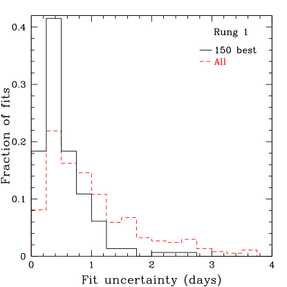
Recall that in lin11 only 150 lens systems were used to project cosmological constraints, and this had strong leverage. If we use only 150 systems in a given rung, choosing those with lowest $\sigma(\widetilde{\Delta t})/|\widetilde{\Delta t}|$, then we obtain precisions ranging from 1.6% (rung 0) to 3.5% (rung 4). The average accuracy over all rungs is $-0.11\%$, and over the four rungs with three day mean cadence is $-0.02\%$.

Figure 4 shows the improvement in the fit uncertainty. Now rung 1 has 60% (89%) of fits within 0.5 (1.0) days, using the 150 systems with lowest $\sigma(\widetilde{\Delta t})/|\widetilde{\Delta t}|$, compared to the previous 30% (61%) for all systems in the rung. For rung 3 the numbers are 37% (83%), compared to the previous 21% (59%). Table 2 summarizes the statistics for the time delay estimation averaged over the rungs.

Figure 4: The distribution of the time delay fit uncertainty is plotted for the 150 time delay estimations with lowest $\sigma(\widetilde{\Delta t})/|\widetilde{\Delta t}|$ (solid) compared to all (dashed), for rung 1. The set of 150 (which may be sufficient for cosmology leverage) has a significantly more precise distribution.

Average	$\qquad P\qquad$	$\qquad A\qquad$
All rungs	0.027	-0.0011
3 day cadence	0.025	-0.0002

Table 2: Time delay estimation statistics are presented for the 150 time delays with lowest $\sigma(\widetilde{\Delta t})/|\widetilde{\Delta t}|$ in each rung, averaged over either all rungs or all rungs with mean 3 day cadence (rungs 0-3).

V Cosmological Requirements on Accuracy

In this section we aim to quantify requirements on the accuracy of the time delay estimation in order for the time delay distance to be a robust cosmological probe. Requirements on precision can be traded off against more systems, since this is a statistical uncertainty, but an actual bias in the time delay, and hence time delay distance, can mislead our cosmological conclusions.

We adopt the combination of cosmological probes used in lin11 : a strong lensing survey giving 1% distance measurements in each of six lens redshift bins from $z_{l}=0.1$–0.6, together with a midrange supernova survey out to $z\approx 1$ and Planck-quality CMB information on the distance to last scattering and the physical matter density $\Omega_{m}h^{2}$. Such a combination was calculated in lin11 to deliver estimation of $\Omega_{m}$ to within 0.0044, the reduced Hubble constant $h$ to 0.0051, or 0.7%, and the dark energy equation of state today $w_{0}$ to 0.077 and its time variation $w_{a}$ to 0.26.

A bias in the time delay $\Delta t$ leads to a bias in the time delay distance $D_{\Delta t}$ of the same fractional magnitude. If there were no redshift variation of the bias, and the only cosmological constraint came from strong lensing alone, then this would show up purely as an offset $\delta h$ in the derived Hubble constant, of the same fractional magnitude since the Hubble constant sets the distance scale. If we wanted a 1% accurate Hubble constant measurement from strong lensing, we would need to ensure that the time delay bias $A$ was under 0.01. However, in the presence of other cosmological information, from supernovae and CMB, this simple mapping no longer holds. Moreover, the bias $A$ may well be redshift dependent.

The current Time Delay Challenge does not yet incorporate cosmological information in the supplied lightcurves, i.e. there are no lens or source redshifts or image geometries assigned. This is planned for a future challenge. However, we might expect that higher redshift lens systems suffer from increased photometric noise and microlensing, which would affect the time delay estimation, as well as lens modeling (e.g. velocity dispersion measurement) and line of sight mass uncertainties. Therefore we take a phenomenological model of the bias

$$A(z)=A_{0}\,\left(\frac{1+z_{s}}{2.05}\right)^{n}\ .$$ (8)

where $A_{0}$ is the amplitude, normalized to the midrange of the source redshift $z_{s}$ distribution, and $n$ allows us to vary the redshift dependence of the bias. Recall we took bins of lens redshift from $z_{l}=0.1$–0.6, and we assume for simplicity $z_{s}=3z_{l}$ (see lin11 for further discussion).

To propagate the offset in time delay, and hence time delay distance, to the bias on the cosmological parameters we employ the standard Fisher bias formalism knox98 ; linbias . The parameter bias is

$$\delta p_{i}=(F^{-1}){}_{ij}\sum_{z}\frac{\partial D_{\Delta t}}{\partial p_{j}}\,\frac{1}{\sigma^{2}(D_{\Delta t})}\,\Delta D_{\Delta t}\ ,$$ (9)

where $F$ is the Fisher matrix (here for the combined probes) and for simplicity we take a diagonal noise matrix. Note that $A=\Delta D_{\Delta t}/D_{\Delta t}$. The parameter bias will scale linearly with the amplitude $A_{0}$.

Figure 5 plots the cosmology bias of an inaccuracy with $A_{0}=0.01$ for various redshift dependences $n$. Note the nearly equal and opposite behavior of $\Omega_{m}$ and $h$, and $w_{0}$ and $w_{a}$, due to their strong covariances. A redshift independent bias ($n=0$) indeed mostly affects the Hubble constant (and $\Omega_{m}$ from its covariance), while one that increases rapidly with redshift predominantly affects $w_{a}$, since it requires a high redshift lever arm to see the dark energy equation of state time dependence.

Figure 5: Bias in time delay estimation propagates into cosmological parameter bias, with amplitude depending on the size of the misestimation (here $A_{0}=0.01$ and we use the combination of probes mentioned in the text) and its redshift dependence, here taken as having power law index $n$. The parameter bias $\delta p$ as a fraction of the parameter uncertainty $\sigma(p)$ is plotted vs $n$ for the various cosmological parameters.

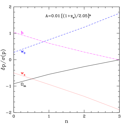
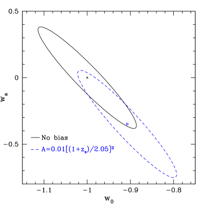
Figure 6 visualizes the cosmology bias caused by such a 1% bias in time delay estimation, for the case of $n=2$. The dark energy equation of state parameters are misestimated such that the derived joint values barely lie within the $1\sigma$ joint confidence contour of the true model, or conversely the true model barely lies within the derived $1\sigma$ joint confidence contour. To avoid such incorrect cosmological conclusions, the time delay must be fit more accurately.

Figure 6: The 68% joint confidence contour for the dark energy parameters $w_{0}$ and $w_{a}$ gets shifted by a 1% time delay estimation bias such that the true cosmology (cosmological constant, marked by x) is near the edge of the contour. The biased value (marked by the square) falsely implies a time varying dark energy.

To impose a time delay accuracy systematic requirement based on controlling cosmological bias, we need to specify in which parameter we are interested and what is the redshift dependence of the systematic. The latter is unknown (though future data challenges may inform this). For example, if the fit bias is proportional to the inverse signal to noise, then this goes as inverse square root of the image flux, or as the luminosity distance. Over the redshift range of interest, in a universe close to $\Lambda$CDM the angular diameter distance is roughly constant with redshift, and so the luminosity distance goes as $(1+z)^{2}$. Thus one might guess $n=2$ is roughly reasonable. We will also be interested in all the cosmological parameters, not just the Hubble constant, say, so we use Fig. 5 in a rule of thumb sense to say that a bias amplitude $A_{0}=0.01$, over a reasonable range of $n$, leads to a roughly $1\sigma$ parameter shift on some cosmological parameter.

We would like the bias to be a small fraction of the statistical uncertainty of the cosmological parameter, $\sigma(p)$. In the presence of both statistical uncertainty and bias, one can use the statistical quantity of the risk,

$$R=\sqrt{(\delta p)^{2}+\sigma^{2}}=\sigma\,\sqrt{1+(\delta p/\sigma)^{2}}\ .$$ (10)

We might ask that the risk increase the error over the statistical contribution by no more than 20%, corresponding to $\delta p/\sigma<0.66$. Since $A_{0}=0.01$ gave $\delta p/\sigma\approx 1$, then this implies we want $A_{0}<0.0066$.

The time delay estimation is not the only contribution to the systematic error budget, however; there is also lens modeling, line of sight mass convergence, etc. so we adopt that the time delay bias – being the most accessible to control – should be less than 1/3 of the total systematic $A_{0}$. Putting this all together we find the requirement that

$$A_{\Delta t} \lesssim \frac{0.01}{3}\,\frac{(\delta p/\sigma)_{\rm desired}}{(\delta p/\sigma)_{A_{0}=0.01}}$$ (11)

$$\lesssim 0.0022\ .$$ (12)

We see from Table 1 that our GP time delay estimation method can satisfy this requirement, except in the case of the six day cadence (rung 4).

VI Conclusions

The time delay distance from strong gravitational lensing multiple images provides a unique, dimensional probe of cosmology. It is directly sensitive to the Hubble constant and has strong complementarity with other probes in determining dark energy characteristics. With new generations of surveys, hundreds to thousands of time delay systems will be found. We investigated one of the leading current sources of uncertainty for this cosmological probe: time delay estimation from noisy, gappy lightcurve data.

Using a Gaussian Process statistical technique we have demonstrated control of systematic bias at the 0.1% level (with precisions at 2.7% for a cosmologically useful data set). The analysis was originally carried out on the blind mock data of the Strong Lens Time Delay Challenge. We have implemented an efficient, completely automated pipeline for fitting thousands of lightcurve systems, with delays from 5-100 days.

The Time Delay Challenge provided data sets with different combinations of mean cadence, cadence variation, season length, and campaign length, allowing us to study their influence on the fits. We find that the number of data points is the most significant influence for delays from 5-100 days, but this can come from either longer seasons or campaigns of more years. For the rare delays of 100 days or more, sufficiently long seasons are crucial. Lengthening the mean cadence raises the systematic bias, with the average three day cadence delivering 0.08% accuracy but a six day cadence degrading this to 0.36%. For a fixed mean cadence, sampling that allows some shorter time monitoring improves the precision.

We investigated the cosmology parameter bias induced by systematic time delay misestimation. Depending on the redshift dependence of the systematic, the major effect is either on the Hubble constant or dark energy equation of state. As a rule of thumb, a 1% total systematic amplitude gives a $1\sigma$ shift in the cosmology. Taking into account the other error contributions this implies that the time delay accuracy requirement should be at the 0.2% level so as not to significantly bias cosmology. The GP fitting technique has demonstrated results sufficient to pass this requirement.

Further improvements are under study. For example, seasons could be weighted by noise to remove periods of bad weather or particularly egregious microlensing. Our GP method delivers the full distributions of hyperparameters, and these could be used to study both the intrinsic variability of the quasar source and the microlensing. The only data provided in the challenge were the lightcurves; future studies could fold in image characteristics and other lens system information.