Abstract

We first discuss Uraltsev’s and other sum rules constraining the $B\to D^{**}(L=1)$ weak transitions in the infinite mass limit, and compare them with dynamical approaches in the same limit. After recalling these well established facts, we discuss how to apply infinite mass limit to the physical situation. We provide predictions concerning semi-leptonic decays and non-leptonic ones, based on quark models. We then present in more detail the dynamical approaches: the relativistic quark model à la Bakamjian-Thomas and lattice QCD. We summarise lattice QCD results in the infinite mass limit and compare them to the quark model predictions. We then present preliminary lattice QCD results with finite $b$ and $c$ quark masses. A systematic comparison between theory and experiment is performed. We show that some large discrepancies exist between different experiments. Altogether the predictions at infinite mass are in fair agreement with experiment for non-leptonic decays contrary to what happens for semileptonic decays. We conclude by considering the prospects to clarify both the experimental situation, the theoretical one and the comparison between both.

Chapter 0 In Memoriam Nikolai Uraltsev :
Uraltsev’s and other Sum Rules, Theory and Phenomenology of $D^{**}$’s

1 In Memoriam of Kolya Uraltsev

In november 2012 we had in Paris a workshop dedicated to $B\to D^{\ast\ast}$ decays. Many of the best specialists of the field were there, experimentalists and theorists. We took time to discuss in detail about what we knew, what was still obscure, how to solve the issues. Among the participants was Kolya Uraltsev. He took a prominent part in the discussions. He was so deep, so rigorous, so strong in his statements, and so careful about the yet unknown, about the ambiguities, so positive about what should be done and about the requests to experimentalists.

We have been working for long on the heavy quark limit for the $B\to D^{\ast\ast}$ decay using a relativistic quark model. In 2000 Kolya derived a very simple and powerful sum rule in the same limit. From there on we started to interact with him. Ikaros Bigi came several times in Orsay and we have published together two “memorinos”. Bigi was a close collaborator and friend of Kolya. Thanks to him we could communicate more intensively with Kolya. All these discussions were really enlightening.

Kolya did not come to our workshop dinner arguing that he would be tempted by the food and that it was not good for him. We did not realise the case was so serious. In February 2013 we received a mail from Ikaros “Dear Friends, on Wednesday (February 13th 2013) Kolya had passed away in Siegen – he was a wonderful person, theorist and true friend. I cannot speak more. Ikaros”. We couldn’t say more either, the shock was too violent.

Now the time has come to honour Kolya by speaking about physics, which was so important for him, to which he devoted all his strength and his admirable brain.

2 Historical elements concerning the discussions about $D^{\ast\ast}$

The issue of the decays $B\to D^{\ast\ast}$ has been actively discussed since more than twenty years under its theoretical and experimental aspects and the relation between both, see [1, 2] for an overlook on these aspects and more recently [3].

1 Well established facts at $m_{Q}\to\infty$

Let us first recall what are the $D^{**}$ under concern. They are the charmed states with quark model assignment $L=1$, and most often we are meaning the lowest lying ones. In the infinite mass limit $m_{Q}\to\infty$, they can be separated into two doublets $j=1/2,j=3/2$, then four states, almost degenerate (except for a small spin orbit force), for each level of excitation. While the $j=1/2$ are broad, the $j=3/2$ are narrow, having respectively $S$ and $D$ waves in pionic decay. The broad $j=1/2$ include a $0^{+}$ and a $1^{+}$, while $j=3/2$ include a $2^{+}$ and a $1^{+}$.

These states are playing a prominent role in the heavy quark sum rules, e.g. the Bjorken sum rule:

$$\rho^{2}=1/4+\sum_{n}(|\tau_{1/2}^{(n)}(w=1)|^{2}+2~{}|\tau_{3/2}^{(n)}(w=1)|^{2})$$ (1)

$n$ labels successive levels of excitation. $\rho^{2}$ is the forward slope of the elastic Isgur-Wise function, while $\tau_{1/2,3/2}$ are similar quantities for the $B\to D^{**}$ transitions [4] . One defines for instance for the $B\to D(0^{+})$ transition:

$$\langle 0^{+}~{}|A_{\lambda}|~{}0^{-}\rangle=-\frac{1}{\sqrt{v_{0}v_{0}^{\prime}}}(v_{\lambda}-v_{\lambda}^{\prime})~{}\tau_{1/2}(w)$$ (2)

where $v,v^{\prime}$ are the four-velocity  vectors of the mesons. $w=v.v^{\prime}$, $w=1$ corresponding to zero recoil. We had observed that this rule is exactly satisfied in a class of quark models [5].

In 2000, N. Uraltsev [6] discovered a new class of sum rules, similar but for the combination of $\tau$’s, which appear now in differences, e.g.:

$$\sum_{n}(|\tau_{3/2}^{(n)}(w=1)|^{2}-|\tau_{1/2}^{(n)}(w=1)|^{2})=1/4$$ (3)

We had found, also from duality arguments, one similar rule [7], except for factors of excitation energy, i.e. the sum has now factors of energy minus the ground state energy :

$$\sum_{n}(E_{3/2}^{(n)}-E_{0})|\tau_{3/2}^{(n)}(w=1)|^{2}-(E_{3/2}^{(n)}-E_{0})|\tau_{1/2}^{(n)}(w=1)|^{2})=...$$ (4)

It is retrieved by the systematic approach of N.Uraltsev in a whole series of sum rules with increasing powers of these energy differences.

At this point, one enters into what will be the main worry in the rest of the chapter. Both rules were indicating an important trend for the $\tau$’s : that one should have $|\tau_{3/2}|$ on the whole larger than $|\tau_{1/2}|$. This is yet a vague statement, which receives a stricter form under the assumption, put forward by N.Uraltsev, that the lowest level (noted $n=0$) is dominating the sums. Then :

$$|\tau_{3/2}^{(0)}(w=1)|>|\tau_{1/2}^{(0)}(w=1)|.$$ (5)

One must be aware that for the deduction to be valid, the dominance must be rather strict.

The statement 1sur3 is precisely the conclusion we had obtained , in the heavy quark limit, from our Bakamjian-Thomas (BT) relativistic quark model approach in the heavy quark limit (shortly described in secBT), some years before.

Another, related, point is that, combining the Uraltsev sum rule ur, with the Bjorken one, one gets a stronger bound on $\rho^{2}$:

$$\rho^{2}>3/4$$ (6)

We had also observed previously that precisely this bound is obtained in the “Bakamjian-Thomas” approach. And, in fact, we have also shown that the Uraltsev sum rule is exactly satisfied in the model [8].

One sees easily that the difference between $\tau_{3/2}(1)$ and $\tau_{1/2}(1)$ is a relativistic effect. Indeed, in an expansion in terms of the light quark internal velocity, $v/c$, $\tau_{3/2}(1)$ and $\tau_{1/2}(1)$ are of order $c/v$, they have the form of dipole transitions where the current matrix element is $\propto\vec{r}\propto m~{}c/v$ and does not depend on the spin. Then, in the non-relativistic limit $\tau_{3/2}(1)-\tau_{1/2}(1)=0$. The difference is subleading in the expansion, and the Uraltsev sum rule displays this : $1/4$ is subleading. But why is the difference positive ?

This type of quark model offers a very simple and intuitive explanation of the difference: one ends with the simple expression

$$\tau_{3/2}(1)-\tau_{1/2}(1)={1\over 2}\int_{0}^{\infty}dp\ p^{2}\ \phi_{1}(p)\frac{p}{p_{0}+m}\phi_{0}(p)$$ (7)

$\phi_{L}(p)$ are the radial wave functions. For simplicity, we have taken $\phi_{1}(p)$ the same for all four states, which amounts to neglect a small spin-orbit force. The two functions $\phi_{0}(p),\phi_{1}(p)$ have been chosen positive by a choice of the phase of states, and the $\tau$’s are then positive. This choice is possible for the lowest states, but not for the $L=1$ radially excited states, for which there are zeroes in the radial wave functions.

The ${\cal O}(v/c)$ factor $\frac{p}{p_{0}+m}$ comes from the Wigner rotation of the light (spectator) quark spin which acts differently on $(1/2)^{+}$ and $(3/2)^{+}$ states. This Wigner rotation is a typical relativistic effect in bound states [9].

It is of order ${\cal O}(v/c)$, which gives indeed ${\cal O}(v/c)^{0}$ for the difference of squares in Uraltsev sum rule (recall that each term squared is ${\cal O}(v/c)^{-2}$). This is compatible with the $1/4$ in the r.h.s of ur : $\tau_{3/2}(1)-\tau_{1/2}(1)$ is positive. Moreover it is large in fact, because the velocity of light quarks within mesons is large : relativistic internal quark velocities .

In summary, $\tau_{3/2}(1)-\tau_{1/2}(1)$ is positive and large. Or, as found quantitatively, $\tau_{1/2}(1)$ is small with respect to $\tau_{3/2}(1)$. In fact, using what is the best potential in our opinion, the model of Godfrey and Isgur [10], in the “Bakamjian-Thomas” formalism, we found :

$$\tau_{3/2}(1) = 0.55$$ (8)

$$\tau_{1/2}(1) = 0.225$$ (9)

Of course, the quark model is not meant to be an exact approach..

Only a true QCD calculation can allow a safe conclusion, therefore it is very important that the conclusion was indeed confirmed later in lattice QCD, at $N_{F}=0$ and then at $N_{F}=2$. The latest result is in final.

One notes that the agreement of the quark model with lattice is very good for $j=3/2$ (central lattice value $\simeq 0.53$), but that it is slightly worse for $j=1/2$ : with the lattice central value ($\simeq 0.3$), quark model is sizeably below, and in squares, which are relevant in the above sum rules and for the rates, the ratio between $\tau_{1/2}(1)$ from lattice and the same from the relativistic quark model is not far from $2$ : $1.7$. Still the close agreement between these estimates for $\tau_{3/2}(1)$ and the semiquantitative agreement for $\tau_{1/2}(1)$ is striking and gives us confidence in these figures.

The advantage of lattice QCD is also that one can estimate errors, since one has now a systematic approach to the true result of QCD. By successive improvement of the calculation, one can estimate the errors with respect, for example, to the continuum and chiral limits.

Up to now everything seems consistent and very encouraging. Lattice approach, general heavy quark statements and quark model agree. The lacking protagonist is experiment. And now comes a possible trouble.

2 Phenomenology in the $m_{Q}\to\infty$ approximation

The results in the infinite mass limit can be used in two ways :

either as purely theoretical tests of the consistency of various approaches-e.g. does one get in a model the necessary Isgur-Wise scaling and the normalisation condition $\xi(1)=1$ ? Or, for the lattice approach, where it is not the question, it may be still a practical check of the soundness of the calculation.

or, more ambitiously, it could be relevant for phenomenology, as well as model dependent results like the ones from the quark model, or exact dynamical calculations of lattice QCD, taken in the the $m_{Q}\to\infty$. Here, the initial idea is of course that for heavy flavor physics the heavy quarks $c,b$ could be sufficiently heavy for the heavy quark limit to be applied, and that many advantages are obtained in that limit. First, new general statements and simplifying features, then new properties of the quark model and other approaches. Even for lattice QCD, the $m_{Q}\to\infty$ limit is useful practically because the treatment of the heavy quark line is especially easy (the heavy quark being described by a Wilson line instead of having to solve numerically a Dirac equation).

A striking example of the phenomenological success of the approach is the prediction of broad and narrow $L=1$ $D^{**}$ states, the $j=1/2$ having pure $S$ wave pionic decay, while the $j=3/2$ have it in $D$ wave. One also observes an agreement for $B\to D^{(*)}$ and for $B\to D^{**}(j=3/2)$ (narrow states). In the last case, this is especially true if one averages over the $j$ multiplet.

Then, one would expect also the above hierarchy $j=1/2\ll j=3/2$ to be observed. In fact, there is at present no clear conclusion, after twenty years of experimental effort.

At this stage however, it must be said more precisely how the $m_{Q}=\infty$ predictions, which are well defined by themselves, may be used for real physics, at finite masses.

There is admittedly no compelling procedure. The only real safe way would be to calculate at the finite physical masses, but we miss theoretical tools to do so, or to calculate corrections to the infinite mass limit. Precisely, the hope was in the beginning to simplify the problems by a clever use of the $m_{Q}=\infty$ limit .

Then, one is just proposing recipes, which have succeeded in the above cases $B\to D^{(*)},D^{**}(j=3/2)$. To be specific, among the many choices of form factors, what are the ones that we assimilate to their $m_{Q}=\infty$ limit ? Different choices will lead to different results for the physical predictions from the same heavy quark theory.

In our papers, we have made a choice based on tau. This means that one keeps the same expression, but with physical velocities. There is at least some logic in using invariant form factors defined with velocity coefficients. The exact formula at finite masses duely contains two independent form factors, which one defines also with velocity factors :

$$\langle 0^{+}~{}|A_{\lambda}|~{}0^{-}\rangle=\frac{1}{2\sqrt{v_{0}v_{0}^{\prime}}}((v_{\lambda}+v_{\lambda}^{\prime})~{}g_{+}(w)+(v_{\lambda}-v_{\lambda}^{\prime})~{}g_{-}(w))$$ (10)

with $g_{+}(w)\propto 1/m_{Q}$ and $g_{-}(w)=-2~{}\tau_{1/2}(w)+{\cal O}(1/m_{Q})$. What we do is to cancel plainly the ${\cal O}(1/m_{Q})$ in $g_{+,-}(w)$, i.e. we set $g_{+}(w)=0,g_{-}(w)=-2~{}\tau_{1/2}(w)$.

It is useful to quote the differential rate corresponding to ff0plus for later discussion:

$$\frac{d\Gamma}{dw}=|V_{cb}|^{2}\frac{G_{F}^{2}~{}m_{B}^{5}}{48\pi^{3}}r^{3}(w^{2}-1)^{\frac{3}{2}}[(1+r)g_{+}-(1-r)g_{-}]^{2}$$ (11)

with $r=m_{D}^{**}/m_{B}$.

3 Semileptonic decays ; the beginning of controversies about the $j=1/2$ states

The predictions have been formulated for integrated rates. Indeed, the semileptonic data were not initially sufficiently accurate to make a comparison for differential distributions. Note that, for the safer lattice QCD, at $m_{Q}=\infty$, one is restricted to $w=1$ and the semileptonic data are not sufficiently accurate to make a comparison in differential distributions around $w=1$ even now. Therefore, one is led to use the quark model even presently.

One obtains for the semileptonic rate of $j=3/2$ in the above mentioned quark model [9], with the choice of Godfrey and Isgur as the best potential model :

$$BR(B\to D^{(\ast\ast)}(j=3/2)2^{+}\,l\,\nu) = 0.70\,\%\qquad D^{\ast}_{2}$$ (12)

$$BR(B\to D^{(\ast\ast)}(j=3/2)1^{+}\,l\,\nu) = 0.45\,\%\qquad D_{1}$$ (13)

$$BR(B\to D^{(\ast\ast)}(j=3/2)\,l\,\nu) = 1.15\,\%$$ (14)

while for $j=1/2$:

$$BR(B\to D^{(\ast\ast)}(j=1/2)1^{+}\,l\,\nu) = 0.07\,\%\qquad D^{\ast}_{1}$$ (15)

$$BR(B\to D^{(\ast\ast)}(j=1/2)0^{+}\,l\,\nu) = 0.06\,\%\qquad D^{\ast}_{0}$$ (16)

$$BR(B\to D^{(\ast\ast)}(j=1/2)\,l\,\nu) = 0.13\,\%$$ (17)

We have indicated on the right the identification of the considered $D^{(**)}$ with the experimental states in the notations of [11], terms although the notations with $j=1/2,3/2$ seem to us much more transparent. Note that the inequality $BR(j=1/2)\ll BR(j=3/2)$ is much stronger that the one between $\tau$’s, first because one has squares, second because there is an additional kinematical factor in the rates.

$$\frac{d\Gamma_{1/2}/dw}{d\Gamma_{3/2}/dw}=\frac{2}{(w+1)^{2}}\left(\frac{\tau_{1/2}(w)}{\tau_{3/2}(w)}\right)^{2}$$ (18)

where one has summed within the $j$ multiplets. The kinematical ratio $\frac{2}{(w+1)^{2}}$ adds a factor $<1/2$ to the ratio $\left(\frac{\tau_{1/2}(w)}{\tau_{3/2}(w)}\right)^{2}$.

While $j=3/2$ states are in rough agreement with experiment from the beginning, especially the sum, $j=1/2$ ones were strongly disagreeing with the results of Delphi, table 10 in [12] at LEP : a large signal was found there for a broad $1^{+}$, an order of magnitude larger than the prediction in 1+ : $BR(B\to D^{\ast}_{1}\,l\,\nu)=(1.25\pm 0.025\pm 0.027)\%$. The $0^{+}$ was not clearly seen : $BR(B\to D^{\ast}_{0}\,l\,\nu)=(0.42\pm 0.33\pm 0.22)\%$.

We have noted that the lattice QCD number for $\tau_{1/2}(1)$ is somewhat higher than the quark model. Therefore, one would expect larger predictions for $BR(B\to D^{\ast}_{1}\,l\,\nu)$ by a factor around two, which would still leave the Delphi data unexplained.

Of course, the discrepancy could originate in the $m_{Q}\to\infty$ approximation. Therefore, very early, general estimates of ${\cal O}(1/m_{Q})$ corrections have been given by Leibovich et al. [13], in a very careful discussion. Concerning $j=1/2$, as well as the $j=3/2,1^{+}$ they show that the vanishing of the amplitude at zero recoil which happens in the infinite mass limit is no longer valid at finite masses, while for the $j=3/2,2^{+}$, vanishing at zero recoil stays valid at finite masses (it has a general kinematical origin). Then they predict very small enhancement for the $j=3/2,2^{+}$. The enhancement they predict by an estimate of the subleading $1/m_{Q}$ contributions does not exceed a factor 3 for $j=3/2,1^{+}$ and $j=1/2,0^{+}$ and is numerically very small for $j=1/2,1^{+}$. Their estimate is of course somewhat model dependent.

For the $0^{+}$, one can understand rather simply that a large enhancement is possible from rate0plus, through a series of effects ( following the discussion in [14]). Now $g_{+}\neq 0$. The contributions from $g_{-}$ and $g_{+}$ add algebraically and may be interfering constructively as found from HQET for first order correction at zero recoil and also in the quark model. The contribution of $g_{-}$ is maintained close to its $m_{Q}\to\infty$ limit according to the quark model, while $g_{+}$ becomes sizable (in fact the BT model finds it rather large, but it is doubtful since it outpasses the ${\cal O}(1/m_{Q})$ magnitude predicted by HQET near zero recoil). The $g_{+}$ contribution is enhanced relatively to the latter by the factor $(1+r)/(1-r)$. All these effects are squared in the rate. The predicted enhancements deserve consideration, but do not correspond to the conclusions of DELPHI, which point to a very large $1^{+},1/2$. We will return to this issue of finite mass corrections when speaking about lattice results at finite masses.

Unexpectedly, the new experiments at the two B factories have not clarified the experimental situation. Quite on the contrary : they have added new contradictions : contradictions within experiment for the same semileptonic reaction, and others between the semileptonic and the non leptonic transitions, newly measured (see below). And the latter were found rather in agreement with the expectations from the $m_{Q}\to\infty$ approximation.

4 Nonleptonic decay. Class I and class III

Indeed, a new, very interesting piece of data has appeared with the measurement of the $B\to D^{**}$ transitions, first by CLEO. Namely the quasi-two body decays $B\to D^{**}\pi$. And it has been realised first from a paper by Neubert [15] that there was a close connection with the semileptonic decay. Indeed through “factorisation” (i.e. the old SVZ “vacuum insertion”), the $B\to D^{**}\pi$ amplitude can be related to the $B\to D^{**}$ current matrix element.

$$B\to D^{**}\pi=f_{\pi}p_{\pi}^{\mu}<D^{**}|J_{\mu}|B>$$ (19)

and then the latter to the semileptonic amplitude. In fact the $B\to D^{**}\pi$ rate is found to be :

$$\frac{\Gamma(\bar{B}^{0}\to H_{c}^{+}\pi^{-})}{{\mathrm{d}}\Gamma(\bar{B}^{0}\to H_{c}^{+}\ell^{-}\bar{\nu})/{\mathrm{d}}q^{2}\Big{|}_{q^{2}=0}}=6\pi^{2}f_{\pi}^{2}\,|V_{ud}|^{2}\,|a_{1}|^{2}+O\left(\frac{M_{\pi}^{2}}{M_{B}^{2}}\right)$$ (20)

where $H_{c}$ is any charmed meson, and where $a_{1}$ is very close to 1. The statement is approximate because factorisation is only an (intuitive and uncontrolled) approximation. Moreover, the formula fact applies properly to the decay $B^{0}\to D^{**-}\pi^{+}$. For $B^{+}\to\bar{D}^{**0}\pi^{+}$, there is another important diagram contributing, obtained by Fierz transformation, with $B\to\pi$ current matrix element and the emission of the $\bar{D}^{**0}$ described by the annihilation constant $f_{D^{**}}$. One distinguishes the two type of decays as being repectively “class I” and “class III” decays. Only class I decay is directly calculable from the $B\to D^{**}$ current matrix element. These decays are discussed in detail in [16].

Let us then first consider this simplest case of class I. The predictions of the quark model with Godfrey-Isgur wave functions in the $m_{Q}\to\infty$ approximation are then [3] :

$$B\left(\overline{B}^{0}\to D_{2}^{3/2\ +}\pi^{-}\right)=11\times 10^{-4}$$

$$B\left(\overline{B}^{0}\to D_{1}^{3/2\ +}\pi^{-}\right)=13\times 10^{-4}$$

$$B\left(\overline{B}^{0}\to D_{1}^{1/2\ +}\pi^{-}\right)=1.1\times 10^{-4}$$ (21)

$$B\left(\overline{B}^{0}\to D_{0}^{1/2\ +}\pi^{-}\right)=1.3\times 10^{-4}.$$

This time, in contrast with the semileptonic case, they were found in rather good agreement with the Belle experiment, the first to give an analysis of the four states. In particular, the striking dissymetry $BR(j=1/2)\ll BR(j=3/2)$ was observed. Finite mass corrections have been estimated according to the procedure of Leibovich et al. and one has found conclusions similar to the semileptonic case [16]. Namely, only the $0^{+}$ is expected to be affected by a large possible enhancement. Rather recently, the $0^{+}$ was also measured by Babar, with a larger rate but much larger errors, then not modifying the initial conclusion, see tab:dsstarpi

Then about class III. There comes one more statement in the $m_{Q}\to\infty$ limit : $f_{D}^{**}(j=3/2)=0$ while $f_{D}^{**}(j=1/2)$ is not all suppressed. A rough estimate shows that for $j=1/2$, the contribution with $f_{D}^{**}$ is large and wins over the class I, which is suppressed, and that it has the same sign [16].

A consequence of this is that class III should be almost the same as class I for $3/2$, but differ strongly for $1/2$. The suppression of $1/2$ predicted and observed in class I should not be present in class III. An estimate from the same paper [16] is :

$$B\left(B^{-}\to D_{2}^{3/2\ 0}\pi^{-}\right)=(8.7\pm 3.2)\times 10^{-4}$$

$$B\left(B^{-}\to D_{1}^{3/2\ 0}\pi^{-}\right)=(10.2\pm 2.3)\times 10^{-4}$$

$$B\left(B^{-}\to D_{1}^{1/2\ 0}\pi^{-}\right)=(7.5\pm 1.7)\times 10^{-4}$$

$$B\left(B^{-}\to D_{0}^{1/2\ 0}\pi^{-}\right)=(9.1\pm 2.9)\times 10^{-4}\ .$$ (22)

This agrees with what is observed tab:dsstarpi.

It is now worth describing and discussing in more details the two dynamical approaches at our disposal, with their properties at physical masses as well as at $m_{Q}=\infty$, and then the present experimental situation.

3 Quark model

One big advantage of the quark model in the present discussion is that it provides well defined predictions for all values of $w$, including the infinite mass limit where it can thus complement the lattice approach. Among the many quark models, we are privileging here a particular approach because of its remarkable properties, and especially those - but not only those - which hold in the $m_{Q}=\infty$ limit.

1 General framework of Bakamjian-Thomas

The Bakamjian-Thomas approach may seem unfamiliar especially because the name itself is unfamiliar, but nevertheless it has been used and developped and promoted to a certain extent among nuclear physicists [17] Its null-plane version has been extensively promoted in particle physics, starting as it seems from M. Terent’ev [18]. We believe that the form with standard quantization on t=0 plane is nevertheless the closest to the intuitions of the quark model. The main idea, starting from the researches of Foldy, is to formulate a relativistic quantum mechanics with a fixed number of particle and an instantaneous interaction. Of course, this is not fully possible, but already what is obtained is significant and it seems to be the best one can do to implement relativity while maintaining the three-dimensional spirit of the quark model.

Indeed, what is obtained is the full set of operators satisfying the Poincaré algebra, which enables to define states in motion from states at rest; the latter being described by wave functions which are eigenvectors of the mass operator.

One can define two sets of dynamical variables : one of global variables, describing the state as whole, $\vec{P},\vec{R},\vec{S}$ ($\vec{R}=-i\partial/\partial\vec{P}$ ), and one of internal variables, in fact the internal momenta ${\vec{k}_{i}}$ (with $\sum_{i=1}^{n}\vec{k}_{i}=\bf{0}$), the conjugate positions, and the spins $\vec{s}_{i}$, with global variables commuting with internal ones.

The mass operator M must be a rotation invariant function of internal variables only, and then commutes with $\vec{P},\vec{R},\vec{S}$.

The Poincaré generators are constructed from the global operators and the interaction in a very simple form. i. e. they have the same form as for a free particle, except that the mass (which appears in $H$ and the generator of Lorentz transformations $\vec{K}$) is replaced by the mass operator M for the bound states

$$\vec{J} = \vec{P}\times-i\partial/\partial\vec{P}+\vec{S}$$ (23)

$$H = \sqrt{M^{2}+\vec{P}^{2}}$$ (24)

$$\vec{K} = 1/2~{}[H,-i\partial/\partial\vec{P}]_{+}-\frac{\vec{P}\times\vec{S}}{H+M}$$ (25)

2 Matrix elements of currrents

One looses relativity when one writes matrix elements of some current between multiquark states (see for details the paper [19]).

Multiquark states in motion are described by first writing a wave function in terms of internal variables :

$$\phi_{s_{1},...s_{n}}(\vec{k}_{1},...\vec{k}_{n})\qquad$$ (26)

These are solutions of the eigenvalue equation $M\phi=m~{}\phi$. Then, the full wave functions in terms of the usual one-particle variables

$$\Psi^{(\textbf{P})}_{s_{1},...s_{n}}(\vec{p}_{1},...\vec{p}_{n})\qquad\qquad\sum_{i=1}^{n}\vec{p}_{i}=\vec{P}$$ (27)

are obtained

by including a plane wave $\delta(\sum_{i}\vec{p}_{i}-\vec{P})$,

by expressing the internal variables in terms of the one-particle variables, which is obtained by a free-quark boost operation (with quark energy $p_{i}^{0}=\sqrt{|\vec{p_{i}}|^{2}+m_{i}^{2}}$), including Wigner rotation of spins $s_{1},...s_{n}$ and Jacobian factors ensuring unitarity. Whence the matrix element of a one-body operator.

If one chooses as current operators standard one quark operators like $1_{i},\sigma_{i},...$ for simplicity and to comply with the basic notion of additivity, then such matrix elements do not respect covariance. In fact, only multibody current operators could implement the covariance. Neither do the one-body currents satisfy the standard Ward identities like vector current conservation.

The remarkable fact is that in the infinite mass limit of one quark, the main difficulties disappear : one finds covariance, current conservation, and also many properties required in this limit : Isgur-Wise scaling, normalisation $\xi(w)=1$, a certain set of sum rules, namely those implying only the Isgur-Wise functions (like the ones of Bjorken and Uraltsev). Also, one finds that in this limit, there is in fact equivalence with a null plane formalism, with a suitable relation between the wave functions at rest and on the null plane.

It is quite possible to calculate in the BT approach at physical masses. However, for the present, in view of the above many difficulties concerning the current matrix elements, and of the many advantages of the heavy mass limit, it is logical to prefer using this limit, with the procedure described in section historical to connect it with phenomenology, keeping in mind that non neglible ${\cal O}(1/m_{Q})$ corrections are expected, especially for the transition to $0^{+}$ (see subsection SL).

3 Choice of the potential model

To fix entirely the model, one needs of course to specify the mass operator $M$, which means the potential model or wave equation at rest. i.e., we choose first the general structure:

$$M=\sum_{i}\sqrt{\vec{k}_{i}^{2}+m_{i}^{2}}+V$$ (28)

Then, we make specifically the choice of the model of Godfrey et Isgur (GI) [10] for the reason that it has been tested with success on a very large range of states, which is less the case for others. We have checked that the qualitative conclusions are general, by making calculations with other models. We think however that in the present problem, where the wave function matters much, the model of Godfrey et Isgur should be preferred also for the following reason : we have noted a sensitivity to the short-distance behavior of the potential for $\tau_{1/2}(w=1)$. With the potential of Veseli and Dunietz [20], which has a strong Coulomb-like potential, one obtains a notably smaller value. The GI model has a duely softened Coulomb-like potential.

In summary, we claim to use a relativistic approach to the quark model. The meaning is twofold : 1) one aspect is the relativistic boost, which allows to treat large velocities of each hadron as a whole. 2) one other is the choice of the internal kinetic energy. It means that the internal velocities may be large.

Still other relativistic aspects, which we do not detail, have been included in the potential $V$ by Godfrey and Isgur.

4 Fundamental methods for QCD : lattice QCD

There has not been many lattice caculations of $B\to D^{\ast\ast}$ decay amplitudes. In the infinite mass limit only the calculation at $w=1$ seems doable. As we shall see the results are in good agreement with the prediction of the Bakamjian-Thomas model.

Only recently the study at finite $b$ and $c$ mass has been undertaken. They have to overcome very noisy signals and only preliminary results can now be presented.

1 Lattice calculation in the infinite mass limit

A preliminary calculation [21] was performed to test a new method. The infinitely massive quarks are described on the lattice by Wilson lines in the time direction. The heavy quark is at rest. Thus one can only consider the $w=1$ case in which the initial and final heavy quarks are both at rest. However, the weak interaction matrix element vanishes at zero recoil. We overcome this problem using formulae from Leibovitch et al. [13]

$$\langle H^{\ast}_{0}(v)|A_{i}D_{j}|H(v)\rangle=i\,g_{ij}\left(M_{H^{\ast}_{0}}-M_{H}\right)\tau_{\frac{1}{2}}(1).$$ (29)

and

$$\langle H^{\ast}_{2}(v)|A_{i}D_{j}|H(v)\rangle=-i\sqrt{3}\left(M_{H^{\ast}_{2}}-M_{H}\right)\tau_{\frac{3}{2}}(1)\epsilon^{\ast}_{ij}\;.$$ (30)

where the $H,H^{\ast}_{0},H^{\ast}_{2}$ are the pseudoscalar, scalar and tensor mesons in the infinite mass limit (the mass differences are finite) and $\epsilon^{\ast}_{ij}$ is the polarisation tensor of $H^{\ast}_{2}(v)$ and $v$ is the four-velocity. $A_{i}$ is the axial vector and $D_{j}$ is the covariant derivative which we know how to discretize on the lattice. Let us skip the details of the lattice calculation. The result of this “quenched” lattice calculation [21] was

$$\tau_{1/2}(1)=0.38(4)(?)\quad{\rm and}\quad\tau_{3/2}(1)=0.53(8)(?)\;,$$ (31)

where the question mark represent unknown systematic errors. A similar calculation was performed later [22, 23] using gauge configurations of the European twisted mass collaboration with $N_{f}=2$ (two light quarks in the see). The calculation has used several values of the light quark masses and one lattice spacing. The result is

$$\tau_{1/2}(1) = 0.296(26)\quad,\quad\tau_{3/2}(1)=0.526(23)$$ (32)

$$\frac{\tau_{3/2}(1)}{\tau_{1/2}(1)} = 1.6\ldots 1.8\quad,\quad\Big{|}\tau_{3/2}(1)\Big{|}^{2}-\Big{|}\tau_{1/2}(1)\Big{|}^{2}\approx 0.17\ldots 0.21$$ (33)

As already mentioned it is really close to the quark model result, eq:BTres. It is also noticeable that the ground state saturates about 80 % of Uraltsev’s sum rule, ur.

2 Lattice calculation with finite $b$ and $c$ masses

The lattice calculation with finite masses is reported in [24, 25]. The calculation is performed using also the gauge configurations of the European twisted mass collaboration with $N_{f}=2$. The calculation is performed with two lattice spacings, one value for the charmed meson mass and three values for the “$B$” meson : 2.5 GeV, 3. GeV and 3.7 GeV.

The mass spectrum of $D^{\ast\ast}$ states

The first issue is to check the mass spectrum predicted by lattice against experiment and to try to relate them with the $j=1/2$ and $j=3/2$ states of the infinite mass limit. It is obvious that the $D^{\ast}_{0}$ ($D^{\ast}_{2}$) corresponds the $j=1/2$ ($j=3/2$) in the ininifte mass limit. It is not so clear for the $J=1$ states which mix $j=1/2$ and $j=3/2$. This study has been performed carefully by Kalinowski and Wagner [26]. They find the first (second) excitation to be dominated by the $j=1/2$ ($j=3/2$) contribution and they are identified to the broad $D_{1}(2430)$ (narrow $D_{1}(2420)$). In [24] an attemp to check the continuum limit for the $D^{\ast}_{0}$ and $D^{\ast}_{2}$ masses is not successful.

The $B\to D^{\ast}_{0}$ at zero recoil

Using twisted quarks the $D^{\ast}_{0}$ can mix with the pseudocalar $D$. We need to isolate both states using the generalised eigenvalue problem (GEVP). In section SL it is mentioned that the $B\to D^{\ast}_{0}$ at zero recoil, which vanishes in the infinite mass limit, might give non vanishing results with finite mass [13]. As discussed in SL the size of this zero recoil contribution is obviously an important issue as it could enhance significantly the $B\to D^{\ast}_{0}l\nu$ branching ratio, improving the agreement with experiment for the semileptonic decay but maybe spoiling the non leptonic one, see phenNL. The preliminary study in [24, 25] has thus concentrated on the zero recoil $B\to D^{\ast}_{0}l\nu$ decay, leaving the full study for later.

Amplitude ratios $B\to D^{\ast}_{0}$ over $B\to D$ lattice spacing (fm) ratio $\boldsymbol{m_{b(1)}}$ ratio $\boldsymbol{m_{b(2)}}$ ratio $\boldsymbol{m_{b(3)}}$ ratio at physical B 0.085(3) 0.33(5) 0.24(4) 0.16(4) 0.06(4) 0.069(2) 0.40(4) 0.31(4) 0.20(4) 0.09(4) continuum 0.55(16) 0.45(17) 0.29(18) 0.15(20) We give the amplitude ratios $B\to D^{\ast}_{0}$ over $B\to D$ at zero recoil, averaged over what seems a good plateau : 6-9 (5-11) for lattice spacing $a=0.085$ fm ($a=0.069$ fm). The $b$ quarks range from the lightest to heaviest from left to right : $m_{B}\simeq 2.5,3,3.7$ GeV. The right column corresponds to the extrapolation at the physical $B$ mass, 5.2 GeV. The last line corresponds to the extrapolation to the continuum. The results are shown in tab:ratioDscalD. From these number we get several conclusions

For the “$B$ meson” masses used and finite lattice spacing the ratios are significant.

But they decrease with increasing $B$ mass leading to a small signal/noise ratio at the physical $B$ mass

The extrapolation to the continuum increases the noise leading to more than 100 % uncertainty. We can thus conclude that there is really a significant zero recoil $B\to D^{\ast}_{0}$ over $B\to D$ amplitude ratio which however, when extrapolated to the physical situation is too uncertain. The situation should improve using a third smaller lattice spacing and larger statistics.

Possible interpretation of $D^{\ast}_{0}$ as a scattering state :

Mohler et al. [27] consider the possible interpretation of the $D^{\ast}_{0}$ as a $D\,\pi$ scattering state. Indeed, what is identified as $D^{\ast}_{0}$ is a broad structure which is certainly strongly coupled to the $D\,\pi$ channel. Under this hypothesis, the study of the $B\to D^{\ast}_{0}l\nu$ should be totally reconsidered.

Figure 1: One example of ratio of the $B\to D^{*}_{2}$ amplitude over the value derived from the infinite mass limit, once the zero recoil has been subtracted. The “B meson mass” is 2.5 GeV and the lattice spacing 0.069 fm. The momentum of the B meson correponds to $w=1.3$. The blue cross corresponds to the discrete representation $E^{+}$ for the $D^{*}_{2}$ interpolating field, $D_{i}V_{i}$, while the red bar corresponds to the discrete representation $T_{2}^{+}$ i.e. $D_{i}V_{j},j\neq i$. The global average is the purple star.

The $B\to D^{\ast}_{2}$ amplitude compared to the infinite mass limit

The $B\to D^{\ast}_{2}$ decay amplitude vanishes at zero recoil. This is obvious in the continuum since a spin 0 particle cannot decay into a spin 2 one via Axial matrix elements which carry spin 0 or 1. However, when using twisted mass quarks, the parity symmetry is violated. The twisted quarks are gathered into isospin doublets and even the heavy quarks are represented in fake “isospins”. There exists an exact symmetry valid at finite lattice spacing consisting in a parity symmetry combined with the flip of the isospin. Thus combining both isospins one gets decay amplitudes which vanish at zero recoil. Of course statistical fluctuations make them not zero. However these fluctuations at zero recoil and non zero recoil are correlated. Thus we can reduce the fluctuations by subtracting the zero recoil result from the non zero recoil result.

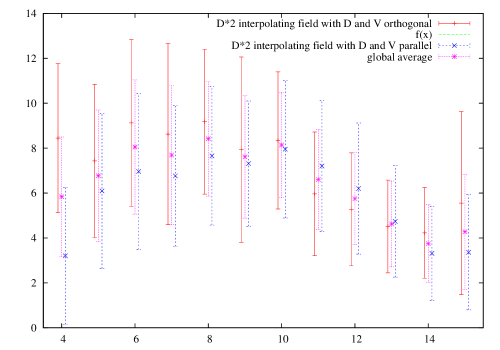
As a benchmark we use the prediction of the infinite mass limit formula. We show in fig:ratioB2D2 one example of such a ratio. A spin 2 meson has 5 possible polarisation. On a lattice these are decomposed into two different discrete symmetry groups : $E^{+}$ and $T_{2}^{+}$. $E^{+}$ corresponds to appropriate combinations of terms of the type $D_{i}\,V_{i}$ where $D_{i}$ is the discretised covariant derivative and $V_{i}$ the vector current, and $T_{2}^{+}$ corresponds to an apropriate combination of terms of the type $D_{i}\,V_{j};j\neq i$, see [24] for more details.

fig:ratioB2D2 shows that there is definitely a signal and the agreement between $E^{+}$ and $T_{2}^{+}$ is rewarding. However the ratio is very large. Since the infinite mass formula agrees rather well with experiment we would expect a ratio closer to 1. This is not the case, the ratio is one order of magnitude larger than 1 and this does not seem to improve when going towards the physical B mass neither towards continuum. The reason for this problem is not yet understood.

5 Experiment

1 Non leptonic versus semileptonic

These respective processes present advantages and drawbacks with respect to each other, so that, on the whole, they should be considered complementary. Indeed:

$\alpha$) On the one hand, semileptonic data have have a series of theoretical advantages. They are directly connected with the matrix elements of the currents, which are the true theoretical objects under study. Non leptonic processes can be related to them only trough the additional assumption of factorisation, which has not a very strong theoretical foundation, although it seems to work well in similar decays like $B\to D^{(*)}\pi$. Moreover, in Class III they are complicated by the additional diagram with $D^{**}$ emission. And in Class I, $B\to D\pi\pi$ contains a non exotic, strongly resonating $\pi^{+}\pi^{-}$ channel which must be extracted off.

$\beta$) One could also believe that the larger branching ratios of semileptonic decays ($10^{-3}$ versus $10^{-4}$) should give them a big superiority in statistics. However, this is overcompensated by far by the fact that the detection efficiency of semileptonic decay is much worse. One has four bodies in the final state instead of three, and a neutrino among them. Finally, the non leptonic data are much more accurate. It is only from them that one has been able to determine the mass and width of the broad states.

Note that one cannot consider the two processes as truly independent, because of their relation through factorisation.

2 Narrow versus broad states

The narrow states $j=3/2$ have always shown quite a good consistency among experimental measurements. And as already said, the theoretical numbers have complied with experiment.

On the other hand, for the broad $j=1/2$, the experimental situation, instead of becoming clearer, has fallen into a real state of confusion. Indeed, aside from the attempts by Delphi at LEP, who found a very large contribution of the broad $1^{+}$ in semileptonic decay, the higher luminosity B factories could be expected to clear up the question; in fact, contrasting results have been obtained by Belle and Babar, with different situations for $0^{+}$ versus $1^{+}$ and for non leptonic versus semileptonic processes.

The fact that narrow states results are quite consistent, while those for broad states are not, suggests that it is the broadness which could be responsible for the difficulties encountered for these states. Indeed, they are very broad : around $300$ MeV. It is also why we shall present separately the experimental result for the two type of states.

3 Results

We begin, in an unusual way, with the non leptonic decay because the situation is clearer, and also to insist on the often underestimated necessity to take them into account for the discussion of the $j=1/2$ case. Since there is compatibility between Belle and Babar where both have measured, we quote only in tab:dsstarpi their averaged results.

Nonleptonic data $j=3/2,1/2$ Decay channel $B_{d}^{0},~{}Class~{}I$ $B^{+},~{}Class~{}III$ $\overline{D}_{2}^{*}\pi^{+}$ $(0.49\pm 0.07)\times 10^{-3}$ $(0.82\pm 0.11)\times 10^{-3}$ $\overline{D}_{1}^{3/2}\pi^{+}$ $(0.82_{-0.17}^{+0.25})\times 10^{-3}$ $(1.51\pm 0.34)\times 10^{-3}$ $\overline{D}_{1}^{1/2}\pi^{+}$ $<1\times 10^{-4}$ $(0.75\pm 0.17)\times 10^{-3}$ $\overline{D}_{0}^{*}\pi^{+}$ $(1.0\pm 0.5)\times 10^{-4}$ $(0.96\pm 0.27)\times 10^{-3}$ Non leptonic branching ratios $B\to D^{\ast\ast}\pi$ averaged between Belle and Babar [28, 30, 29, 31, 32].The final strong decay branching fractions have been taken as detailed footnote 6 of [3].

One notes the remarkable fact that in Class I, $j=1/2$ are one order of magnitude smaller than $j=3/2$, while all have the same order of magnitude $10^{-3}$ in Class III. This is explained clearly by theory, see above, phenNL.

For the Class I, the following warnings must be made :

• the large uncertainty ($50\%$) in the $0^{+}$ case, is due to the fact that Babar has an appreciably larger value, but with a very large uncertainty. This very large uncertainty is itself due to the uncertainty in the extraction of a non resonant contribution.

• the $1^{+},j=1/2,3/2$ ($D^{*}\pi$ channel) have been measured only by Belle.

Semileptonic data $j=3/2$ Decay channel $Belle$ $Babar$ $\overline{D}_{2}^{*}~{}l\nu$ $(0.54\pm 0.12)\times 10^{-2}$ $(0.39\pm 0.11)\times 10^{-2}$ $\overline{D}_{1}^{3/2}~{}l\nu$ $(0.93\pm 0.22)\times 10^{-2}$ $(0.64\pm 0.15)\times 10^{-2}$ Semileptonic branching ratios for B semileptonic decay into narrow states, from Belle and Babar. See HFAG [33] and references therein. The final strong decay branching fractions have been taken as detailed footnote 6 of [3]. For semileptonic decays we quote first the results of $j=3/2$ (narrow states) in tab:SLnarrow : Obviously, the two experiments are here quite compatible.

Semileptonic data $j=1/2$ Decay channel $Belle$ $Babar$ $\overline{D}_{1}^{1/2}~{}l\nu$ $<1.05\times 10^{-3}$ $(0.40\pm 0.05)\times 10^{-2}$ $\overline{D}_{0}^{*}~{}l\nu$ $(0.36\pm 0.09)\times 10^{-2}$ $(0.42\pm 0.09)\times 10^{-2}$ Semileptonic branching ratios for B semileptonic decay into broad states, from Belle and Babar. See HFAG [33] and references therein. The final strong decay branching fractions have been taken as detailed footnote 6 of [3]. The semileptonic decay into $j=1/2$ from Babar and Belle is reported in tab:SLbroad : There is a strong disagreement for the $1^{+}(1/2)$ between the two experiments while the results for $0^{+}$ are quite compatible

About $0^{+}$ : one could say that in view of the agreement between the two experiments in the semileptonic case, we might trust this large result. But given the rather direct relation between semileptonic and Class I non leptonic decays, and the strong suppression of $0^{+}$ in non leptonic (see the above tab:dsstarpi), this conclusion would be very doubtful.

The general conclusion could be that, not surprisingly, the very broad states raise more difficulties precisely because of their broadness.

6 Conclusion : discussion on theory and experiment, prospects

1 Discussion on theory and experiment

One must say that the non leptonic data, tab:dsstarpi, seem to support strongly theoretical expectations coming from the $m_{Q}\to\infty$ approximation:

1) suppression of $j=1/2$ with respect to $j=3/2$ in Class I, by one order of magnitude. The agreement with GIclassI is semiquantitative for both $j$, and good if summing over the members of the $j$ multiplets.

2) This suppression is no more present in Class III, due to the diagram with $D^{**}$ which is large in the $j=1/2$ case, but not for $j=3/2$, also from a statement of $m_{Q}\to\infty$ limit. Indeed [16] one observes that the $j=1/2$ are strongly enhanced in class III, by one order of magnitude, and the $j=3/2$ much more slightly (the two diagrams can be shown to add constructively).

The $j=3/2$ semileptonic data are much larger, as expected from the $m_{Q}\to\infty$ approximation, and in quantitative agreeement when averaging over the members of the multiplet.

The only definite discrepancy with theory in the $m_{Q}\to\infty$ limit is in the semileptonic case, for the $j=1/2,0^{+}$ state, where the two experiments agree. It could be understood as coming from the broadness of the states and the lower detection efficiency of semileptonic measurements, rendering the identification of the resonance still more difficult (much less observed events) .

Of course, part of the discrepancy could be due to the $1/m_{Q}$ corrections being large. This can be suggested by the finding of Leibovich et al., that precisely this transition can suffer more $1/m_{Q}$ enhancement. This effect could combined with the fact that lattice QCD finds a somewhat larger $\tau_{1/2}(1)$ than our quark model (see well). But then, it would remain to explain the non leptonic data : why then $0^{+}$ seems so small in Class I. Therefore, still something would remain problematic on one or another side of experiment.

Another problem is the large Babar result for the broad $1^{+},1/2$ (contrasting with the small one from Belle). It would be a real worry if confirmed, because in this case one does not expect any serious enhancement according to the calculations of Leibovich et al. (the conclusion is the same in the quark model [14]).

2 Prospects

• The most urgent problem seems the experimental one :

  1) to solve the discrepancy between the two B factory, see tab:SLbroad, concerning the semileptonic decay to $1^{+}(j=1/2)$

  2) to clarify the discrepancy which seems to exist between the semileptonic and the Class I non leptonic data for the $0^{+}$ ($j=1/2$) (tab:dsstarpi and tab:SLbroad), if we believe factorisation. There is a strong suppression in the latter with respect to the $j=3/2$, while $0^{+}$ is of the same order as $j=3/2$ in semileptonic. It would be already very useful to reduce the uncertainty of Babar measurement of the Class I non leptonic decay for the $0^{+}$, and to have the Babar measurement of the $1^{+}(j=1/2)$ partner.

  It would also be very useful to complement the study of the broad states by the one of their strange counterparts, which are narrow, and therefore much easier to identify. This is proposed in the article [3].

  On the other hand, on the theoretical side :

• since one can “fear” unexpectedly large $1/m_{Q}$ corrections in the $0^{+}$, lattice QCD at finite mass should be developped as much as possible. For the moment lattice calculations at finite mass make it very likely that a significant zero recoil contribution to $B\to D^{\ast}_{0}$ is there. However the extrapolation to the physical situation leads to more than 100 % uncertainty, tab:ratioDscalD. This of course is not the case for $B\to D^{\ast}_{2}$ but there the ratio of the finite mass signal over the infinite mass estimate is larger than expected and than experiment for an unknown reason. The progress will come from using additionally a smaller lattice spacing to make safer the continuum limit, to look in detail into the momentum dependance of all these decays and to chase possible remaining artefacts.

• since one needs anyway other approaches, mainly the quark model, to understand things at large $w$ (for example $q^{2}=0$ for the pionic weak transition), one should try to improve estimates of $1/m_{Q}$ corrections.

• Finally, to justify the longstanding efforts dispensed on the problem, both from the part of theorists and of experimentalists, it must be said why it seems so important to clarify the situation for $L=1,~{}j=1/2$. It is because, on the whole, a serious issue is the phenomenological relevance of the $m_{Q}=\infty$ approach in $b\to c$ decay. This limit has been considered very attractive because allowing several important new theoretical statements, in particular the sum rules, which deeply involve theses states ; and at the same time, it has met quite encouraging phenomenological successes in $B\to D^{(*)}$ and $B\to D^{**},L=1,~{}j=3/2$ transitions, as well as in the strong decays $D^{**}\to D^{(*)}\pi$ with both $j=1/2$ and $j=3/2$.

  Of course it is expected that the results of $m_{Q}=\infty$ are a better approximation for the $j=3/2,2+$ state than for the other cases. Indeed, in the latter cases, the no recoil amplitude at $m_{Q}=\infty$ vanishes contrary to general expectation, and a non zero value should be present, resulting from $1/m_{Q}$ effects. Indeed, theoretical expectations from certain identities lead to possible large effects at order ${\cal O}(1/m_{Q})$ in the $1+,3/2$ and $0^{+}$ cases. Unluckily, lattice are not yet able to answer clearly to their size at physical masses, and whether they could fill the large gap with presently observed value for the $0^{+}$ in the semileptonic decay . Moreover, such a large non zero value at no recoil which would mean an S-wave between the final $D^{\ast\ast}$ and the $l\nu$ system, is to be confronted to the success of the $m_{Q}=\infty$ approximation for the class I non-leptonic decays. Can this S-wave effect be damped in the maximal recoil kinematics which is that of the $D^{\ast\ast}\pi$ ? Models rather point to a soft variation of the corresponding effect.

• This longstanding efforts are also finally justified by the important side effect that the decays considered here have on the estimate of $V_{cb}$.

References

- 1. Memorino on the ‘ versus puzzle’ in . I.I. Bigi, B. Blossier, A. Le Yaouanc, L. Oliver, O. Pene, J.-C. Raynal, A. Oyanguren, P. Roudeau. e-Print: hep-ph/0512270
- 2. I.I. Bigi, B. Blossier, A. Le Yaouanc, L. Oliver, O. Pene, J.-C. Raynal, A. Oyanguren, P. Roudeau. Memorino on the ‘ versus puzzle’ in : A Year Later and a Bit Wiser. Published in Eur.Phys.J.C52:975-985,2007. e-Print: arXiv:0708.1621 [hep-ph]
- 3. Proposal to study transitions Damir Becirevic, Alain Le Yaouanc, Luis Oliver, Jean-Claude Raynal (Orsay, LPT), Patrick Roudeau (Orsay, LAL), Justine Serrano (Marseille, CPPM). Jun 2012. 13 pp. Published in Phys.Rev. D87 (2013) 5, 054007 e-Print: arXiv:1206.5869 [hep-ph]
- 4. N. Isgur and M. B. Wise, Phys. Rev. D 43 (1991) 819.
- 5. Exact duality and Bjorken sum rule in heavy quark models a la Bakamjian-Thomas, A. Le Yaouanc, L. Oliver, O. Pene, J.C. Raynal Phys.Lett. B386 (1996) 304-314 e-Print: hep-ph/9603287
- 6. N. Uraltsev, Phys. Lett. B 501 (2001) 86 [hep-ph/0011124].
- 7. A. Le Yaouanc, L. Oliver, O. Pene, J. C. Raynal and V. Morenas, PoS HEP 2001 (2001) 082 [hep-ph/0110372].
- 8. Uraltsev sum rule in Bakamjian-Thomas quark models, A. Le Yaouanc, L. Oliver, O. Pene, J.C. Raynal , V. Morenas, Phys.Lett. B520 (2001) 25-32 e-Print: hep-ph/0105247
- 9. V. Morenas, A. Le Yaouanc, L. Oliver, O. Pene and J. C. Raynal, Phys. Rev. D 56 (1997) 5668 [hep-ph/9706265].
- 10. S. Godfrey and N. Isgur, Phys. Rev. D 32 (1985) 189.
- 11. K. Nakamura et al. (Particle Data Group), J. Phys. G 37, 075021 (2010) and 2011 partial update for the 2012 edition.
- 12. J. Abdallah et al. [DELPHI Collaboration], Eur. Phys. J. C 45 (2006) 35 [hep-ex/0510024].
- 13. A. K. Leibovich, Z. Ligeti, I. W. Stewart and M. B. Wise, Phys. Rev. D 57 (1998) 308 [hep-ph/9705467].
- 14. Finite mass corrections to transitions in the Bakamjian-Thomas approach,A. Le Yaouanc, L. Oliver, J. C. Raynal (to be published).
- 15. Theoretical analysis of decays. M. Neubert. Published in Phys.Lett.B418:173-180,1998. e-Print: hep-ph/9709327
- 16. The Decays and the Isgur-Wise functions , . F. Jugeau, A. Le Yaouanc, L. Oliver, J.-C. Raynal, Published in Phys.Rev.D72:094010,2005. e-Print: hep-ph/0504206
- 17. B. Keister, W. Polyzou, Adv. Nucl. Phys.20, 225 (1991).
- 18. M. Terent’ev Sov. J.Nucl. Phys. 24, 106 (1971).
- 19. Covariant quark model of form-factors in the heavy mass limit, A. Le Yaouanc, L. Oliver, O. Pene, J.C. Raynal, Phys.Lett. B365 (1996) 319-326
- 20. S. Veseli and I.Dunietz Phys. Rev. D54 6803 (1996)
- 21. D. Becirevic, B. Blossier, P. Boucaud, G. Herdoiza, J. P. Leroy, A. Le Yaouanc, V. Morenas and O. Pene, Phys. Lett. B 609 (2005) 298 [hep-lat/0406031].
- 22. B. Blossier et al. [European Twisted Mass Collaboration], JHEP 0906 (2009) 022 [arXiv:0903.2298 [hep-lat]].
- 23. B. Blossier et al. [ETM Collaboration], PoS LAT 2009 (2009) 253 [arXiv:0909.0858 [hep-lat]].
- 24. M. Atoui, B. Blossier, V. Morenas, O. Pene and K. Petrov, arXiv:1312.2914 [hep-lat].
- 25. M. Atoui, arXiv:1305.0462 [hep-lat].
- 26. M. Wagner and M. Kalinowski, arXiv:1310.5513 [hep-lat].
- 27. D. Mohler, S. Prelovsek and R. M. Woloshyn, Phys. Rev. D 87, no. 3, 034501 (2013). [arXiv:1208.4059 [hep-lat]].
- 28. B. Aubert et al., BaBar Collaboration, Phys. Rev. D79 112004, 2009. [arXiv:0901.1291 [hep-ex]].
- 29. P. del Amo Sanchez et al., BaBar Collaboration, SLAC-PUB-14203, e-Print: arXiv:1007.4464 [hep-ex]. PoS ICHEP 2010 (2010) 250
- 30. K. Abe et al., Belle Collaboration, Phys. Rev. Lett. 94 221805, 2005. K. Abe et al. [Belle Collaboration], [hep-ex/0410091].
- 31. K. Abe et al., Belle Collaboration, Phys. Rev. D69 112002, 2004. [hep-ex/0307021].
- 32. A. Kuzmin et al., Belle Collaboration, Phys. Rev. D76 012006, 2007. et al. [Belle Collaboration], [hep-ex/0611054].
- 33. D. Asner et al. [Heavy Flavor Averaging Group Collaboration], arXiv:1010.1589 [hep-ex].