Verifiable UML Artifact-Centric Business Process Models

Abstract

Artifact-centric business process models have gained increasing momentum recently due to their ability to combine structural (i.e., data related) with dynamical (i.e., process related) aspects. In particular, two main lines of research have been pursued so far: one tailored to business artifact modeling languages and methodologies, the other focused on the foundations for their formal verification. In this paper, we merge these two lines of research, by showing how recent theoretical decidability results for verification can be fruitfully transferred to a concrete UML-based modeling methodology. In particular, we identify additional steps in the methodology that, in significant cases, guarantee the possibility of verifying the resulting models against rich first-order temporal properties. Notably, our results can be seamlessly transferred to different languages for the specification of the artifact lifecycles.

1 Introduction

A business process consists of several activities performed in coordination in order to achieve a business goal [21]. Since business processes are key to achieving an organization’s goals, they should be free of errors and performed in an optimal way.

Traditional approaches to business process modeling have been based on a process- or activity-centric perspective, that is, they have tended to focus on the ordering of the activities that need to be carried out, underspecifying or ignoring the data needed by the process.

An alternative to activity-centric process modeling is the artifact-centric (or data-centric) approach. Artifact-centric process models represent both structural (i.e. the data) and dynamic (i.e. the activities or tasks) dimensions of the process. For this reason, they have grown in importance in recent years. One of the research lines in this topic is focused on finding the best way of representing artifact-centric process models. Several graphical alternatives have been proposed, such as Guard-Stage-Milestone (GSM) models [14], BPMN with data [17], PHILharmonic Flows [16] or a combination of UML and OCL [8], to mention a few examples.

Despite this variety, it is important to guarantee the correctness of these models. In order to do so, a second line of research has focused on the foundations for the formal verification of artifact-centric business process models. The greatest part of these works represent the business process using models grounded on logic, such as Data-centric Dynamic Systems (DCDS) [1, 2, 5]. However, the problem with these models grounded on logic is that they are not practical at the business level as they are complex and difficult to understand by the domain experts.

In this paper, we merge these two lines of research, by showing how recent theoretical decidability results for verification can be fruitfully transferred to a concrete UML-based modeling methodology. In particular, we identify sufficient conditions over the models used by this methodology which guarantee decidabilty of verification. We also show how decidability of verification can be achieved when one of such conditions is not fulfilled. These results represent a significant step forward in the area since, to our knowledge, this is the first time that conditions for decidability are stated on models understandable by model experts, which are specified at a high level of abstraction.

As an aside result of our work, we identify a particular class of models, called shared instances, characterized by the fact that there are two (or more) artifacts which share a read-only object. In this particular case, decidability is achieved by limiting the number of static objects with which an artifact can be related, by ensuring that all queries are navigational starting from the artifact and by imposing that no path of associations among two classes is navigated back and forth. Under these conditions, we can achieve decidability of verification without having to restrict reasoning over a bounded number of artifacts. More importantly, these results are not only applicable to our UML and OCL models, but can be extended to other languages for artifact-centric process models that fulfill the same conditions.

The rest of the paper is structured as follows. Section 2 introduces our framework. Section 3 presents our example, over which we will show the decidability conditions. Section 4 reports the decidability results. Finally, Sections 5 and 6 review the related work and present our conclusion.

2 The BAUML Framework

To facilitate the analysis of artifact-centric business process models, we base our work on the BALSA framework [13]. It establishes four different dimensions that should be present in any artifact-centric business process model:

• Business Artifacts: Business artifacts represent the data that the business requires to achieve its goals. They have an identifier and may be related to other business artifacts. One way of representing business artifacts is by using an entity-relationship model or a UML class diagram. Both diagrams are able to represent the business artifacts, their relationships and establish constraints on both.

• Lifecycles: Lifecycles are used to represent the evolution of an artifact during its life, from the moment it is created until it is destroyed. Intuitively, they can be graphically represented by means of statecharts or state machine diagrams.

• Services: Services are atomic units of work in the business process. They are in charge of evolving the process. As such, they make changes to artifacts by creating, updating and deleting them. They may be represented in different ways: alternatives range from using natural language to logic or with operation contracts specified in OCL.

• Associations: Associations establish restrictions on the way services may change artifacts, that is, they impose constraints on services. They may be represented using a procedural representation, such as a workflow or BPMN, or using a declarative representation, such as condition-action rules.

In contrast to artifacts, whose evolution we wish to track, in many instances, businesses need to keep data in the system that does not really evolve. In order to distinguish this data from artifacts, we will refer to it as objects.

In this paper, we adopt the instantiation of BALSA in [8, 9], representing the aforementioned dimensions using UML [15] and OCL [19]. Both UML and OCL are standard languages generally used for, but not limited to, conceptual modeling. In particular, we use: UML class diagrams for artifact, object, and relationship types; UML state machine diagrams for artifact lifecycles; UML activity diagrams for associations, and OCL operation contracts for services. We call this concrete modelling approach BALSA UML (BAUML for short). However, this does not restrict our result to this subset of diagrams: the results are extendable to the rest of alternatives.

Technically, we define a BAUML model $\mathcal{B}$ as a tuple $\langle\mathcal{M},\mathcal{O},\mathcal{S},\mathcal{P}\rangle$, where:

• $\mathcal{M}$ is a UML class diagram, in which some classes represent (business) artifacts. Given two classes $A$ and $B$, we say that $A$ is a $B$, written $A\sqsubseteq_{\mathcal{M}}B$, if $A=B$ or $A$ is a direct or indirect subclass of $B$ in $\mathcal{M}$. Furthermore, given a class $A$ and a (binary) association $R$ in $\mathcal{M}$, we write $A=_{\mathcal{M}}\exists R$ ($A=_{\mathcal{M}}\exists R^{-}$ resp.) if $A$ is the domain of $R$ (image of $R$ resp.) according to $\mathcal{M}$. We also denote by $R|_{1}$ and $R|_{2}$ the role names attached to the domain and image classes of $R$. We denote the set of artifacts in $\mathcal{M}$ as $\textsc{artifacts}(\mathcal{M})$ and, when convenient, we use $\textsc{artifacts}(\mathcal{B})$ interchangeably. Each artifact is the top class of a hierarchy whose leaves are subclasses with a dynamic behavior (their instances change from one subclass to another). Each subclass represents a specific state in which an artifact instance can be at a certain moment in time. We denote by $\textsc{a-classes}(\mathcal{M})$ ($\textsc{a-classes}(\mathcal{B})$ resp.) the set of such subclasses, including the artifacts themselves. Given a class $\texttt{S}\in\textsc{a-classes}(\mathcal{M})$, we denote by $\textsc{art}_{\texttt{S}}$ the class S itself if S is an artifact, or the class A if A is an artifact and S is a possibly indirect subclass of A. Given an artifact $\texttt{A}\in\textsc{artifacts}(\mathcal{M})$, we denote by $\textsc{a-states}(\texttt{A})$ the set of leaves in the hierarchy with top class A.

• $\mathcal{O}$ is a set of OCL constraints over $\mathcal{M}$.

• $\mathcal{S}$ is a set of UML state transition diagrams, one per artifact in $\textsc{artifacts}(\mathcal{M})$. In particular, for each artifact $\texttt{A}\in\textsc{artifacts}(\mathcal{M})$, $\mathcal{S}$ contains a state transition diagram $S_{\texttt{A}}=\langle V,v_{0},E,T\rangle$, where $V$ is a set of states, $v_{0}\in V$ is the initial state, $E$ is a set of events, and $T\subseteq V\times E\times\mathit{OCL}_{\mathcal{M}}\times V$ is a set of transitions between pairs of states, each labelled by an event in $E$ and by an OCL condition over $\mathcal{M}$. In particular, the states $V$ of $S_{\texttt{A}}$ exactly mirror the classes in $\textsc{a-states}(\texttt{A})$, so that $S_{\texttt{A}}$ encodes the allowed event-driven transitions of an artifact instance of type A from the current state to a new subclass (i.e., a new artifact state). Moreover, the initial transitions leading to $v_{0}$ always result in the creation of an instance of the artifact being specified by $S_{\texttt{A}}$.

• $\mathcal{P}$ is a set of UML activity diagrams, such that for every transition diagram $\langle V,v_{0},E,T\rangle\in\mathcal{S}$, and for every event $\varepsilon\in E$, there exists one and only one activity diagram $P_{\varepsilon}\in\mathcal{P}$. With a slight abuse of notation, given a state transition diagram $S\in\mathcal{S}$, we denote by $\mathcal{P}_{S}\subseteq\mathcal{P}$ the set of activity diagrams referring to all events appearing in $S$.

In this paper, we will not impose any restriction on the control-flow structure of such activity diagrams, but only on their atomic tasks and conditions. For this reason, given an artifact $\texttt{A}\in\textsc{artifacts}(\mathcal{M})$, we respectively denote by $\textsc{tasks}(\texttt{A})$ and $\textsc{conditions}(\texttt{A})$ the set of atomic tasks and conditions appearing in the state transition diagram $S_{a}$, also considering all activity diagrams related to $S_{\texttt{A}}$. We then define $\textsc{tasks}(\mathcal{B})=\bigcup_{\texttt{A}\in\textsc{artifacts}(\mathcal{M})}\textsc{tasks}(\texttt{A})$ and $\textsc{conditions}(\mathcal{B})=\bigcup_{\texttt{A}\in\textsc{artifacts}(\mathcal{M})}\textsc{conditions}(\texttt{A})$. Moreover, we assume that every task in $\textsc{tasks}(\texttt{A})$ that does not belong to the activity diagram of an initial transition takes in input an instance of the artifact type in $S_{a}$ and that every condition in $\textsc{conditions}(\texttt{A})$ is in the scope of such artifact.

In BAUML, conditions are expressed as OCL queries over the UML class diagram $\mathcal{M}$. Similarly, each (atomic) task is associated to a so-called operation contract, which expresses a precondition on the executability of the task, and a postcondition describing the effect of the task, both formalized in terms of OCL queries over $\mathcal{M}$. The semantics of the operation contract is that the task can only be executed when the current information base satisfies its precondition, and that, once executed, the task brings the information base to a new state that satisfies the task postcondition. In this light, tasks represent services in the terminology of BALSA.

3 Example

We present a relevant example based on a system for a company that registers orders from customers, and stores information about the orders made by the company to its suppliers. Our example is likely to specify a simplified version of the artifact-centric process models of an online shop like Amazon. We use a set of UML diagrams and OCL operation contracts to represent the example in a modeler-friendly way according to the BALSA framework.

Figure 1 shows the class diagram that represents the business artifacts and classes of our example. Artifacts are characterized by having several substates, represented as subclasses, with a disjointness constraint. This constraint is necessary to ensure that each artifact evolves correctly. In addition, artifacts have a lifecycle, in our case represented as a UML state machine.

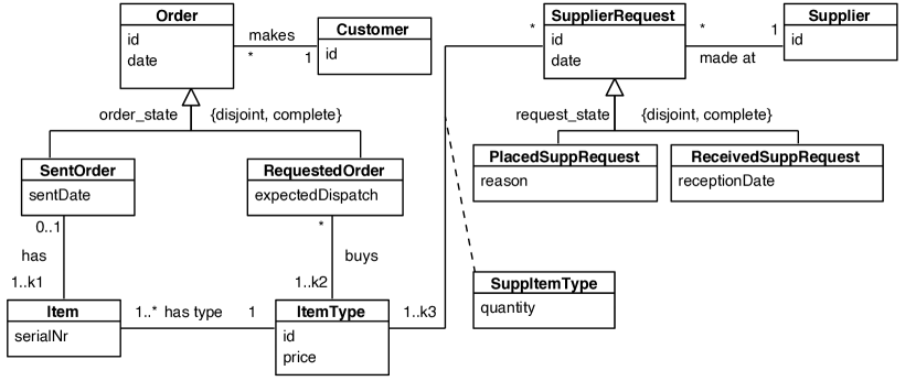
Key constraints: serialNr for Item, id for the other classes.

Figure 1: Class diagram for our example

Logically, business artifacts, objects and associations to which they participate are created, updated, and destroyed by executing different services or tasks. However, we assume that some classes/associations are read-only, i.e., their extension is not changed by the processes. This is the case, e.g., for ItemType in our example. Figure 1 shows two business artifacts: Order and SupplierRequest. Order has two substates: RequestedOrder and SentOrder, that track the order’s evolution. A RequestedOrder is related to various ItemTypes, indicating the products that the customer wishes to purchase. On the other hand, SentOrder is related to Items, which have a certain ItemType. That is, SentOrders are directly related to specific items identified by their serial number. Notice that apart from the artifact itself, the associations makes, has, and buys in which it takes part, are also created and deleted by the process.

Similarly, SupplierRequest represents the requests made to the supplier. It has two possible substates: PlacedSuppRequest and ReceivedSuppRequest, and it is related to ItemType, the association class that results from this relationship states information about the quantity of items of a certain type that have been requested to the supplier.

We call the artifact structure in this example shared instances by two artifacts (shared instances for short), because multiple artifacts (even of a different type) can be associated to the same object. While an object might be related to an arbitrary number of artifact instances, the opposite does not hold, i.e., we naturally model an upper bound on the number of objects to which an artifact instance is related, so as to control the amount of information attached to the same artifact instance (e.g., consider the cardinalities of the buys association in Figure 1).

Order:
 
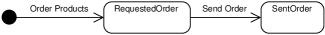
SupplierRequest:
 

Figure 2: Artifact state machines

Both artifacts Order and SupplierRequest evolve independently from each other, with a lifecycle specified by the state machines of Figure 2. Their meaning is very intuitive. In the case of Order, when event Order Products takes place, the RequestedOrder is created. When we have a requested order and event Send Order executes, the order is sent to the customer and the artifact changes its state to SentOrder. The state machine diagram for SupplierRequest is analogous to that of Order.

Each of the events in the lifecycle transitions (Order Products, Send Order, Order Products at Supplier and Receive Supplier Order) are further defined using an activity diagram, which shows the units of work (i.e., the tasks) that are carried out, together with their execution order.

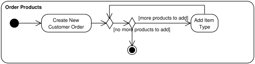
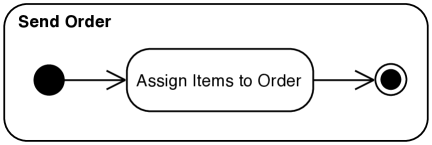
Figure 3: Activity diagrams for the events of Order

Figure 3 shows the activity diagrams for the events of Order. As for the Order Products event, the first task creates a new order, and the second task, which can be executed many times, adds an item type to the order that has been previously created. As for the Send Order event, the task adds the items to the order, marking it as sent.

Each activity diagram only gives an intuitive idea of what each task does. In order to specify tasks formally, we use OCL operation contracts, each of which has a precondition and a postcondition. Below we show the OCL operation contracts for the tasks in Figure 3.
$\scriptsize\begin{array}[]{@{}l@{}}\textbf{action}~{}\mathsf{CreateNewCustomerOrder}\\ ~{}~{}(\mathit{orderId}:\texttt{String},\mathit{date}:\texttt{Date},\mathit{expDisp}:\texttt{Date}):\texttt{RequestedOrder}\\ \textbf{pre:}~{}\mathit{\neg\texttt{RequestedOrder}.allInstances()\rightarrow exists(ro|ro.id=orderId)}\\ \textbf{post:}~{}\mathit{\texttt{RequestedOrder}.allInstances()}\\ \qquad\begin{array}[]{@{}l@{}l@{}}\mathit{\rightarrow exists(ro|}&\mathit{ro.oclIsNew()\land ro.id=orderId\land ro.date=date}\\ &\mathit{{}\land ro.expectedDispatch=expDisp\land result=ro)}\end{array}\end{array}$

$\mathsf{CreateNewCustomerOrder}$ receives as input the necessary parameters to create a new instance of the artifact RequestedOrder. Its precondition makes sure that no other order with the same identifier exists. It returns the RequestedOrder that has been created with the input parameters. This is an example of the kind of operation that is used to create new artifact instances, and that is typically associated to transitions leading to the initial artifact state (Order Products in this example).
$\scriptsize\begin{array}[]{@{}l@{}}\textbf{action}~{}\mathsf{AddItemType}(\mathit{idItemType}:\texttt{String},\mathit{ro}:\texttt{RequestedOrder})\\ \textbf{pre:}~{}\mathit{\neg ro.itemType.id\rightarrow includes(idItemType)}\\ \textbf{post:}~{}\mathit{ro.itemType.id\rightarrow includes(id)}\end{array}$

$\mathsf{AddItemType}$ adds an ItemType to the order that has been created in the previous operation. Its precondition checks that the item type has not been already added to the order, and the postcondition creates the relationship between the given order and the right item type.

Notice that we assume that the artifact instance that is returned by the first operation, $\mathsf{CreateNewCustomerOrder}$, is reused in the following operations. This assumption is necessary to ensure that we are always dealing with the same artifact instance.
$\scriptsize\begin{array}[]{@{}l@{}}\textbf{action}~{}\mathsf{AssignItemsToOrder}(\mathit{o}:\texttt{RequestedOrder},\mathit{date}:\texttt{Date})\\ \textbf{pre:}~{}\begin{array}[t]{@{}l@{}l@{}}\mathit{o.itemType\rightarrow forAll(it|}&\mathit{it.item}\\ &\mathit{\rightarrow exists(i|i.sentOrder\rightarrow isEmpty()))}\end{array}\\ \textbf{post:}~{}\begin{array}[t]{@{}l@{}}\mathit{\neg o.oclIsTypeOf(\texttt{RequestedOrder})\land o.oclIsTypeOf(\texttt{SentOrder})\land{}}\\ \mathit{o.oclAsType(\texttt{SentOrder}).sentDate=date\land{}}\\ \mathit{o.itemType\rightarrow forAll(it|o.oclAsType(\texttt{SentOrder}).item}\\ \mathit{\quad\rightarrow includes(it.item@pre}\\ \mathit{\qquad\rightarrow select(i|i.sentOrder\rightarrow isEmpty()).asOrderedSet()}\\ \mathit{\quad\qquad\rightarrow first()))}\end{array}\end{array}$

$\mathsf{AssignItemsToOrder}$ checks whether for the given RequestedOrder $o$ it is the case that there are available items (i.e., that have not been assigned to a SentOrder) for each of the requested item types. If so, $o$ becomes a SentOrder that is associated to an available item for each of the requested item types.

These operation contracts show that the only elements that are created are the artifact itself and its relationships to other objects. Notice again that class ItemType, which is shared by Order and SupplierRequest, is never modified by the tasks, and is in fact read-only. Moreover, all the actions that are not attached to the initial transition take as input an instance of the artifact type whose evolution is being modelled in the corresponding state machine, as required by our methodology. Notice that the navigation of all the OCL expressions in the pre and postconditions starts from the instance of the artifact flowing in the state transition diagram: an Order (or one of its subclasses) in our example.

Given a BAUML model, it is interesting to check that it fulfills desired properties that ensure its correctness, such as the artifact termination property: once an artifact instance is created, it should eventually evolve to a terminal state. This is addressed in the next section.

4 Verification of BAUML Models

The purpose of this section is to carefully analyze the interaction between the dynamic and static component of BAUML models, so as to single out the various sources of undecidability when it comes to their verification. We show in particular that all the restrictions we introduce towards decidability of verification are in fact required: by relaxing just one of them, verification becomes again undecidable.

4.1 Verification Logic

To specify temporal properties over BAUML models, we adopt the logic $\mu\mathcal{L}_{p}$, a variant of first-order $\mu$-calculus that has been recently introduced to specify requirements about the evolution of data-aware processes, jointly considering the temporal dimension as well as the data maintained in the different system states [1]. We recap here the main aspects of $\mu\mathcal{L}_{p}$ [1], contextualizing it to the case of BAUML models.

Given a BAUML model $\mathcal{B}$, the logic $\mu\mathcal{L}_{p}$ is defined as:

$$\Phi::=\ Q~{}\mid~{}\lnot\Phi~{}\mid~{}\Phi_{1}\land\Phi_{2}~{}\mid~{}\exists x.\textsc{live}(x)\land\Phi~{}\mid~{}$$

$$\textsc{live}(\vec{x})\land\langle\!{-}\!\rangle\Phi~{}\mid~{}\textsc{live}(\vec{x})\land[\!{-}\!]\Phi~{}\mid~{}Z~{}\mid~{}\mu Z.\Phi$$

where $Q$ is a possibly open FO query, $Z$ is a second order predicate variable, and the following assumption holds: in $\textsc{live}(\vec{x})\land\langle\!{-}\!\rangle\Phi$ and $\textsc{live}(\vec{x})\land[\!{-}\!]\Phi$, the variables $\vec{x}$ are exactly the free variables of $\Phi$, once we substitute to each bounded predicate variable $Z$ in $\Phi$ its bounding formula $\mu Z.\Phi^{\prime}$ [1]. This requirement expresses that $\mu\mathcal{L}_{p}$ quantifies only over those objects/artifacts that persist in the system, i.e., continue to stay in the active domain of the system.

We make use of the following abbreviations:

• $\Phi_{1}\lor\Phi_{2}=\neg(\neg\Phi_{1}\land\neg\Phi_{2})$,

• $[\!{-}\!]\Phi=\neg\langle\!{-}\!\rangle\neg\Phi$,

• $\nu Z.\Phi=\neg\mu Z.\neg\Phi[Z/\neg Z]$,

• $\forall x.\texttt{A}(x)\rightarrow\Phi=\neg(\exists x.\texttt{A}(x)\land\neg\Phi)$,

• $\textsc{live}(\vec{x})\rightarrow\langle\!{-}\!\rangle\Phi=\neg(\textsc{live}(\vec{x})\land[\!{-}\!]\neg\Phi)$,

• $\textsc{live}(\vec{x})\rightarrow[\!{-}\!]\Phi=\neg(\textsc{live}(\vec{x})\land\langle\!{-}\!\rangle\neg\Phi)$.

The last two abbreviations show that $\mu\mathcal{L}_{p}$ allows one to “control” what happens when quantification ranges over a value that disappears from the current active domain: in the $\rightarrow$ case the property trivializes to true, in the $\land$ case it trivializes to false.

Among the properties of interest for BAUML models, we consider in particular the fundamental requirement of artifact termination. Intuitively, this property states that in all possible evolutions of the system, whenever an artifact instance of a certain type is present in the system, it must persist in the system until it eventually reaches (in a finite amount of computation steps) a proper termination state. Remember that such a state will have a counterpart in the UML model of $\mathcal{B}$, which will contain a subclass for that specific state. By denoting with $\textsc{term}_{\texttt{A}}\in\textsc{a-states}(\texttt{A})$ the proper termination state of artifact $\texttt{A}\in\textsc{artifacts}(\mathcal{B})$, and by considering the standard FOL encoding of UML classes as unary predicates, the artifact termination property can be formalized in $\mu\mathcal{L}_{p}$ as follows:

$$\nu Z.\Big{(}\bigwedge_{\texttt{A}\in\textsc{artifacts}(\mathcal{B})}(\forall x.\texttt{A}(x)\rightarrow\mu Y.\textsc{term}_{\texttt{A}}(x)\lor(\texttt{A}(x)\land\langle\!{-}\!\rangle Y))\Big{)}\land[\!{-}\!]Z$$

In the following, all the undecidability results we give do not only hold for the $\mu\mathcal{L}_{p}$ logic in general, but specifically for the artifact termination property. Furthermore, we do only consider data coming from a countably infinite unordered domain, and that can only be compared for (in)equality. We thus avoid any assumption on the structure of data domains, and consider only string and boolean attributes. In this light, our results witness that it is not possible to achieve meaningful restrictions towards decidability just by restricting the property specification logic, but that it is instead necessary to suitably restrict the expressiveness of BAUML models themselves.

Since all the undecidability proofs rely on the encoding of 2-counter machines [18] into the specific class of BAUML models under analysis, we start by briefly recapping 2-counter machines.

4.2 2-Counter Machines

We follow the original formulation in [18]. A counter is a memory register that stores a non-negative integer. Given two positive integers $n,m\in\mathbb{N}^{+}$, an $m$-counter machine $\mathcal{C}$ with counters $c_{1},\ldots,c_{m}$ is a program with $n$ commands:

$$1:\mathit{CMD}_{1};\quad 2:\mathit{CMD}_{2};\quad\ldots\quad n:\mathsf{HALT};$$

where each $\mathit{CMD}_{k}$ (for index $k\in\{1,\ldots,n-1\}$) is either an increment command or a conditional decrement command.

Given $i\in\{1,\ldots,m\}$, an increment command for counter $i$, written $\mathsf{INC}(i,$), is a command that increases the counter $c_{i}$ of one unit, and then jumps to the next instruction. Formally, for $k,k^{\prime}\in\{1,\ldots,n-1\}$,

$$k:\mathsf{INC}(i,k^{\prime})\quad\text{ means }\quad k:c_{i}:=c_{i}+1;~{}\mathsf{GOTO}\ k^{\prime};$$

Given $i\in\{1,\ldots,m\}$, and $k,k^{\prime},k^{\prime\prime}\in\{1,\ldots,n\}$, a conditional decrement instruction for counter $i$ and instruction $k$, written $\mathsf{CDEC}(i,k^{\prime},k^{\prime\prime})$, tests whether the value of counter $i$ is zero. If so, it jumps to instruction $k^{\prime}$; otherwise, it decreases counter $i$ of one unit, and then jumps to instruction $k^{\prime\prime}$. Formally, for $k,k^{\prime},k^{\prime\prime}\in\{1,\ldots,n-1\}$, command $k:\mathsf{CDEC}(i,k^{\prime},k^{\prime\prime})$ means

$$k:\textbf{if}~{}c_{i}=0~{}\textbf{then}~{}\mathsf{GOTO}\ k^{\prime};\textbf{else}~{}\{c_{i}:=c_{i}-1;~{}\mathsf{GOTO}\ k^{\prime\prime};\}\\$$

An input for an $m$-counter machine is an $m$-tuple $\langle d_{1},\ldots,d_{m}\rangle$ of values in $\mathbb{N}$ initializing its counters. Given an $m$-counter machine $\mathcal{C}$ and an input $I$ of size $m$, we say that $\mathcal{C}$ halts on input $I$ if the execution of $\mathcal{C}$ with counter initial values set by $I$ eventually reaches the last, $\mathsf{HALT}$ command.

It is well-known that checking whether a 2-counter machine halts on a given input is undecidable [18], and it is easy to strengthen this result as follows:

Corollary 4.1

It is undecidable to check whether a 2-counter machine halts on input $\langle 0,0\rangle$.

Proof 4.2.

Given a 2-counter machine $\mathcal{C}$ with input $I=\langle d_{1},d_{2}\rangle$, one can produce a new 2-counter machine $\mathcal{C}^{\prime}$ whose program is constituted by the sequence of the following instruction sets:

1. a series of $d_{1}$ commands of type $k:\mathsf{INC}(1,k+1)$;

2. a series of $d_{2}$ commands of type $k:\mathsf{INC}(2,k+1)$;

3. the program of $\mathcal{C}$, whose indexes are translated of $d_{1}+d_{2}$ units.

It is easy to see that $\mathcal{C}$ halts on input $\langle d_{1},d_{2}\rangle$ if and only if $\mathcal{C}^{\prime}$ halts on input $\langle 0,0\rangle$.

In the following, we say that a 2-counter machine halts if it halts on input $\langle 0,0\rangle$.

4.3 Unrestricted Models

We start by showing that, if we do not impose restrictions on the shape of OCL queries used in the pre-/post-conditions of tasks and in the decision points of a BAUML model, then verification of artifact termination is undecidable. We say that a BAUML model is unrestricted if it does not impose any restriction on the shape of such queries.

Theorem 4.3.

Checking termination over unrestricted BAUML models is undecidable.

Proof 4.4.

By reduction from the halting problem of 2-counter machines, which is undecidable (cf. Corollary 4.1). Specifically, given a 2-counter machine $\mathcal{C}$, we produce a corresponding unrestricted BAUML model $\mathcal{B}_{\mathcal{C}}=\langle\mathcal{M}^{u},\emptyset,\{S_{\texttt{2CM}}^{u}\},\{P_{init}^{u},P_{run}^{u}\}\rangle$, whose components are illustrated in Table 1. The idea behind the reduction is as follows. $\mathcal{M}$ contains a single artifact 2CM, which can be ready or halted, the latter being the termination state ($\textsc{term}_{\texttt{2CM}}=\texttt{Halted2CM}$), as it can be clearly seen in $S_{\texttt{2CM}}^{u}$. As specified in diagram $S_{\texttt{2CM}}$, the $\mathsf{init}$ operation is activated only if the extension of Flag is empty. In this case, a new artifact instance of Ready2CM and a new object of type Flag are simultaneously created. The creation of a Flag object has the effect of blocking the possibility of creating new instances of Ready2CM, in turn ensuring that only a single instance of Ready2CM will be created, and that only one execution of $P_{run}$ will run. In fact, the only instance of 2CM that enters $S_{\texttt{2CM}}$ will move to the halted state by executing the activity diagram $P_{run}$. In turn, $P_{run}$ encodes the program of $\mathcal{C}$, by combining the process fragments obtained by translating the single commands in $\mathcal{C}$ as specified in Table 1. Two classes $\texttt{Item}_{1}$ and $\texttt{Item}_{2}$ are used to mirror the two counters. In particular, at a given moment in time, the number of instances of $\texttt{Item}_{i}$ represents the value of counter $i$. In this light: (i) incrementing counter $i$ translates into the creation of a new instance of $\texttt{Item}_{i}$; (ii) testing whether counter $i$ is 0 translates into checking whether the extension of class $\texttt{Item}_{i}$ is empty; (iii) decrementing counter $i$ translates into the deletion of one of the current instances of $\texttt{Item}_{i}$. Table 1 shows how these three aspects can be formalized in terms of activity diagrams and OCL queries (focusing on counter $1$). The diamond gateways at the beginning of each fragment are used to properly merge multiple incoming paths.

The claim follows by observing that $\mathcal{C}$ halts if and only if the unique instance of 2CM that enters $S_{\texttt{2CM}}$ also reaches the $\mathsf{Halted2CM}$ state, i.e., properly terminates.

$\mathcal{M}^{u}$	$S_{\texttt{2CM}}^{u}$

$P_{init}^{u}$		$\mathsf{init}\ \begin{array}[t]{@{}l@{\ }l}\textbf{pre:}&\mathit{\texttt{Flag}.allInstances()\rightarrow isEmpty()}\\ &\land\neg(\texttt{Ready2CM}.allInstances()\rightarrow exists(m^{\prime}|m^{\prime}.id=id))\\ \textbf{post:}&\mathit{\texttt{Flag}.allInstances()\rightarrow exists(f|f.oclIsNew())}\\ &\mathit{\land\texttt{Ready2CM}.allInstances()\rightarrow exists(m|m.oclIsNew()\land m.id=id\land result=m)}\end{array}$

$P_{run}^{u}$	start
	$k:\mathsf{INC}(1,k^{\prime})$		$\mathsf{inc_{1}}\ \begin{array}[t]{@{}l@{\ }l}\textbf{pre:}&\mathit{\neg(\texttt{Item1}.allInstances()\rightarrow exists(i^{\prime}|i^{\prime}.id=id))}\\ \textbf{post:}&\mathit{\texttt{Item1}.allInstances()\rightarrow exists(i|i.oclIsNew()\land i.id=id)}\end{array}$
	$k:\mathsf{CDEC}(1,k^{\prime},k^{\prime\prime})$		$\begin{array}[]{@{}l}Q_{0}^{1}=\mathit{\texttt{Item1}.allInstances()\rightarrow isEmpty()}\\[6.0pt] \mathsf{dec_{1}}\ \begin{array}[t]{@{}l@{\ }l}\textbf{pre:}&\mathit{\texttt{Item1}.allInstances()\rightarrow exists(i|i.id=id)}\\ \textbf{post:}&\mathit{\neg(\texttt{Item1}.allInstances()\rightarrow exists(i|i.id=id))}\end{array}\end{array}$
	$n:\mathsf{HALT}$		$\mathsf{halt}\ \begin{array}[t]{@{}l@{\ }l}\textbf{post:}&\mathit{\neg(m.oclIsTypeOf(\texttt{Ready2CM}))}\\ &\mathit{\land m.oclIsTypeOf(\texttt{Halted2CM})}\end{array}$

Table 1: Unrestricted BAUML model simulating a 2-counter machine

4.4 Navigational and Unidirectional Models

The proof of Theorem 4.3 relies on the fact that artifact instances freely manipulate (i.e., create, read, delete) instances of other classes. Towards decidability, we have therefore to properly control how artifact instances relate to other objects. In this light, we suitably restrict OCL expressions, by allowing only so-called navigational expressions.

To define navigational queries over a BAUML model $\mathcal{B}=\langle\mathcal{M},\mathcal{O},\mathcal{S},\mathcal{P}\rangle$, we start by partitioning the associations and classes in $\mathcal{M}$ into two sets: a read-only set $\mathcal{M}_{r}$, and a read-write set $\mathcal{M}_{rw}$. Intuitively, $\mathcal{M}_{r}$ represents the portion of $\mathcal{M}$ whose data are only accessed, but never updated, by the execution of tasks, whereas $\mathcal{M}_{rw}$ represents the portion of $\mathcal{M}$ that can be freely manipulated by the tasks. These two sets can either be directly specified by the modeler, or easily extracted by inspecting all postconditions of operations present in $\mathcal{P}$, marking a class C as read-write every time a sub-expression $\mathit{obj.oclIsNew()}$ appears in some operation, and $obj$ is an instance of C. In this light, all artifacts presents in $\mathcal{M}$ are always part of the read-write set: $\textsc{artifacts}(\mathcal{M})\subseteq\mathcal{M}_{rw}$.

Given an object $obj$, an OCL expression is navigational from $obj$ if it is defined by means of the usual OCL operations like exists, select, …, but in which each subexpression is a boolean combination of expressions $Q_{i}$ that obey to one of the following two types:

• $Q_{i}$ only uses role and class names from $\mathcal{M}_{r}$;

• $Q_{i}$ has the form of a path $o.r_{1}\cdots r_{n}$, which starts from $o$ and navigates through roles $r_{1}$ to $r_{n}$, where each $r_{i}$ is either a role or an attribute, and where $o$ is either the original object $obj$, or a variable used in the current operation.

A BAUML model $\mathcal{B}=\langle\mathcal{M},\mathcal{O},\mathcal{S},\mathcal{P}\rangle$ is navigational if:

• For every operation in $\mathcal{P}$, with the exception of the $\mathsf{init}$ operation, the OCL expressions used in its pre- and post-conditions are navigational from $a$, where $a$ is (the name of) the artifact instance taken in input by the operation.

• Every condition in $\textsc{conditions}(\mathcal{B})$ is an OCL expression that is navigational from (the name of) the artifact instance present in the scope of the condition.

Navigational BAUML models do not allow artifact instances to share objects from read-write classes. Indeed, for an artifact instance to establish a relation with an object of class C previously created by another artifact instance, it is necessary to write an OCL query that selects objects of type C, but this query is not navigational.

In spite of this observation, we will see that restricting BAUML models to navigational queries is still not sufficient, but additional requirements are needed towards decidability. The first requirement is related to the way OCL expressions navigate the roles in $\mathcal{M}$. Given a navigational BAUML model $\mathcal{B}=\langle\mathcal{M},\mathcal{O},\mathcal{S},\mathcal{P}\rangle$, and given a role $r$ in $\mathcal{M}$, if there exists an OCL expression in $\mathcal{B}$ that mentions $r$, then we say that $r$ is a target role, written $\textsc{trg}_{\mathcal{B}}(r)$, otherwise we say that $r$ is a source role, written $\textsc{src}_{\mathcal{B}}(r)$. We use this notion to define the notion of dependency between two classes. Given classes $\texttt{C}_{1}$ and $\texttt{C}_{n+1}$ in $\mathcal{M}$, we say that $\texttt{C}_{n+1}$ depends on $\texttt{C}_{1}$ if there exists a tuple $\langle A_{1},\ldots,A_{n}\rangle$ of binary associations such that each $A_{i}$ connects $\texttt{C}_{i}$ and $\texttt{C}_{i+1}$, and the role of $A_{i}$ attached to $\texttt{C}_{i+1}$ is a target role. We then say that $\mathcal{B}$ is bidirectional if it is navigational and there exists a class in $\mathcal{M}_{rw}$ that depends on itself or on one of its super/sub-classes, unidirectional if it is navigational and there is no class in $\mathcal{M}_{rw}$ that depends on itself or on one of its super/sub-classes. Intuitively, for a unidirectional BAUML model it is possible to mark each association in its UML model as directed (since no association can have both nodes as targets), and the resulting directed graph is acyclic. See for example Table 2. This property, in turn, can be tested in NLogSpace.

We now correspondingly characterize navigation in $\mu\mathcal{L}_{p}$. Without loss of generality, we consider only binary relations. A pseudo-navigational $\mu\mathcal{L}_{p}$ property has the form

$$\begin{array}[]{@{}l@{}l@{}}\Phi::=&\mathsf{true}\mid\mathsf{false}\mid A(x)\mid\lnot A(x)\mid\Phi_{1}\land\Phi_{2}\mid\Phi_{1}\lor\Phi_{2}\mid\\ &Z\mid\mu Z.\Phi\mid\nu Z.\Phi\mid\\ &\exists x.A(x)\land\Phi(x)\mid\forall x.A(x)\rightarrow\Phi(x)\mid\\ &\exists y.R(x,y)\land\Phi(y)\mid\forall y.R(x,y)\rightarrow\Phi(y)\mid\\ &\exists y.R(y,x)\land\Phi(y)\mid\forall y.R(y,x)\rightarrow\Phi(y)\mid\\ &A(x)\land\langle\!{-}\!\rangle\Phi\mid A(x)\land[\!{-}\!]\Phi\mid A(x)\rightarrow\langle\!{-}\!\rangle\Phi\mid A(x)\rightarrow[\!{-}\!]\Phi\end{array}$$

where, in the last row, variable $x$ is exactly the single free variable of $\Phi$, once we substitute to each bounded predicate variable $Z$ in $\Phi$ its bounding formula $\mu Z.\Phi^{\prime}$ (resp., $\nu Z.\Phi^{\prime}$). Notice that pseudo-navigational properties are in negation normal form, and that they constitute indeed a fragment of $\mu\mathcal{L}_{p}$. In fact, even if they do not make use of live, they always guard quantification and next-state transitions with classes and/or relations, which imply the corresponding quantified objects to be in the current active domain.

Given a unidirectional BAUML model $\mathcal{B}=\langle\mathcal{M},\mathcal{O},\mathcal{S},\mathcal{P}\rangle$, we characterize the fact that a closed, pseudo-navigational $\mu\mathcal{L}_{p}$ property $\Phi$ is navigationally compatible with $\mathcal{B}$ as:

• $\Phi$ contains a subformula of the form $\exists x.A(x)\land\Psi(x)$ or $\forall x.A(x)\rightarrow\Psi(x)$.

• The largest subformula of $\Phi$ of the form $\exists x.A(x)\land\Psi(x)$ or $\forall x.A(x)\rightarrow\Psi(x)$ is such that:

• $A\in\textsc{a-classes}(\mathcal{B})$, and

• $A$ and $x$ are compatible with $\Psi$, written $\textsc{cmp}_{A}^{x}(\Psi)=\mathsf{true}$, according to the notion of compatibility defined below. Given a class $C$ in $\mathcal{M}$, a variable $x$, and a pseudo-navigational open $\mu\mathcal{L}_{p}$ property $\Phi(x)$, we define $\textsc{cmp}_{C}^{x}(\Phi)$ as:

  1. $\mathsf{true}$ if $\Phi\in\{\mathsf{true},\mathsf{false},Z\}$

  2. $C\sqsubseteq_{\mathcal{M}}A\lor A\sqsubseteq_{\mathcal{M}}C$ if $\Phi\in\{A(x),\neg A(x)\}$

  3. $\textsc{cmp}_{C}^{x}(\Phi_{1})\land\textsc{cmp}_{C}^{x}(\Phi_{2})$ if $\Phi\in\{\Phi_{1}\land\Phi_{2},\Phi_{1}\lor\Phi_{2}\}$

  4. $\textsc{cmp}_{C}^{x}(\Psi)$ if $\Phi\in\{\mu Z.\Psi,\nu Z.\Psi\}$

  5. $\mathsf{false}$ if $\Phi\in\{\exists y.A(y)\land\Psi(y),\forall y.A(y)\rightarrow\Psi(y)\}$

  6. $\textsc{trg}_{\mathcal{B}}(R|_{2})\land\textsc{cmp}_{C^{\prime}}^{y}(\Psi)\land((C\sqsubseteq_{\mathcal{M}}\exists R)\lor(\exists R\sqsubseteq_{\mathcal{M}}C))$
     if $\Phi\in\{\exists y.R(x,y)\land\Psi(y),\forall y.R(x,y)\rightarrow\Psi(y)\}$
     and $C^{\prime}=_{\mathcal{M}}\exists R^{-}$

  7. $\textsc{trg}_{\mathcal{B}}(R|_{1})\land\textsc{cmp}_{C^{\prime}}^{y}(\Psi)\land((C\sqsubseteq_{\mathcal{M}}\exists R^{-})\lor(\exists R^{-}\sqsubseteq_{\mathcal{M}}C))$
     if $\Phi\in\{\exists y.R(y,x)\land\Psi(y),\forall y.R(y,x)\rightarrow\Psi(y)\}$
     and $C^{\prime}=_{\mathcal{M}}\exists R$

  8. $(C\sqsubseteq_{\mathcal{M}}A\lor A\sqsubseteq_{\mathcal{M}}C)\land\textsc{cmp}_{C}^{x}(\Psi)$
     if $\Phi\in\{A(x){\land}\langle\!{-}\!\rangle\Psi,A(x){\land}[\!{-}\!]\Psi,A(x){\rightarrow}\langle\!{-}\!\rangle\Psi,A(x){\rightarrow}[\!{-}\!]\Psi\}$

Intuitively, the formulae above state that: (1) $C$ and $x$ are always compatible with non-first-order subformulae. (2) $C$ and $x$ are compatible with first-order components of the form $A(x)$ or $\neg A(x)$ if classes $A$ and $C$ belong to the same hierarchy according to $\mathcal{M}$; this means that navigation through classes is only allowed in the context of the same hierarchy. (3) boolean connectives distribute the compatibility check to all their inner sub-formulae. (4) fixpoint constructs push the compatibility check to their inner sub-formulae. (5) compatibility is broken if new quantified variables over classes are introduced in the formula. This means that at most one quantification over classes is allowed in a pseudo-navigational property to be navigationally compatible with $\mathcal{B}$. (6) and (7) deal with navigation along a binary relation, from the first to the second component in (6), and from the second to the first component in (7). In particular, (6) states that the formula can quantify over the second component of a relation $R$ where $x$ points to the first component if: (i) the second component of $R$ is a target role in $\mathcal{B}$, witnessing that $\Phi$ agrees with the unidirectional navigation imposed by $\mathcal{B}$ over $R$; (ii) class $C$ belongs to the same hierarchy of the domain class for $R$, according to $\mathcal{M}$; (iii) $C^{\prime}$and $y$ are navigationally compatible with the inner formula $\Psi$, where $y$ is the newly quantified variable, and $C^{\prime}$ is the image class for $R$ according to $\mathcal{M}$. (7) works in a similar way, by simply inverting the second and first components of $R$. (8) next-state transition formulae are compatible if the class used in the guard belongs to the same hierarchy of $C$, and $C$ and $x$ are compatible with the inner subformula.

Notice that termination properties are always guaranteed to be navigationally compatible with the corresponding BAUML model, since A and $\textsc{term}_{\texttt{A}}$ belong by definition to the same hierarchy.

Unfortunately, the following result shows that restricting BAUML models to be unidirectional is not sufficient to obtain decidability of checking termination properties.

Theorem 4.5.

Checking termination of unidirectional BAUML models is undecidable.

Proof 4.6.

Given a 2-counter machine $\mathcal{C}$, we produce a corresponding unidirectional BAUML model $\mathcal{B}_{\mathcal{C}}=\langle\mathcal{M}^{*},\emptyset,\{S_{\texttt{2CM}}^{*}\},\{P_{init}^{*},P_{run}^{*}\}\rangle$, whose components are illustrated in Table 2. $\mathcal{M}^{*}$ contains a single artifact 2CM, which can be ready or halted, the latter being the termination state ($\textsc{term}_{\texttt{2CM}}=\texttt{Halted2CM}$), as attested by $S_{\texttt{2CM}}^{*}$. When the $\mathsf{init}$ operation is applied, a new instance $m$ of Ready2CM is created, attaching to it two dedicated objects of type Counter, using respectively role $c1$ and $c2$ of the associations $hasC1$ and $hasC2$. Such Counter objects mirror the two counters of $\mathcal{C}$. In particular, each of the two Counter objects attached to $m$ has a 1-to-many association with Item: at a given time, the number of items attached to $m.c1$ ($m.c2$ resp.) represents the value of the first (second resp.) counter in $\mathcal{C}$.

The artifact instance $m$ then executes the process corresponding to the $\mathsf{run}$ event, which suitably encodes the program of $\mathcal{C}$: (i) incrementing the first counter translates into the inclusion of a new Item to the items of $m.c1$, i.e., to the set $m.c1.items$; (ii) testing whether the first counter is 0 translates into checking whether set $m.c1.items$ is empty; (iii) decrementing the first counter translates into the removal of one item from set $m.c1.items$ (it is not important which). Table 2 shows how these three aspects can be formalized in terms of activity diagrams and OCL queries The management of the second counter is analogous, with the only difference that it involves $m.c2.items$ in place of $m.c1.items$. Figure 4 intuitively shows the evolution of a specific configuration of the system in response to the application of two operations.

Observe that, as graphically depicted in $\mathcal{M}^{*}$ (consistently with the operations), $\mathcal{B}_{\mathcal{C}}$ is unidirectional: all OCL expressions (except from that in $\mathsf{init}$) are navigational in $m$, and navigation unidirectionally flows from 2CM to Counter to Item. Furthermore, no two objects of type Counter, nor two objects of type Item, are shared by different instances of 2CM. This means that every instance of Ready2CM runs the process corresponding to the program of $\mathcal{C}$ in total isolation with other instances of $\texttt{Ready2CM})$ and, consequently, either all halt or none halt. The claim follows by observing that $\mathcal{C}$ halts if and only if all instances of Ready2CM eventually reaches the $\mathsf{Halted2CM}$ state, i.e., properly terminate.

$\mathcal{M}^{*}$	$S_{\texttt{2CM}}^{*}$

$P_{init}^{*}$		$\begin{array}[t]{@{}l@{\ }l}\textbf{pre:}&\neg(\texttt{Ready2CM}.allInstances()\rightarrow exists(m^{\prime}|m^{\prime}.id=id))\\ \textbf{post:}&\mathit{\texttt{Ready2CM}.allInstances()\rightarrow exists(m|\begin{array}[t]{@{}l}m.oclIsNew()\land m.id=id\land result=m\\ {}\land(m.c1\rightarrow exists(c_{1}|c_{1}.oclIsNew()))\\ {}\land(m.c2\rightarrow exists(c_{2}|c_{2}.oclIsNew()))~{})\\ \end{array}}\\ \end{array}$

$P_{run}^{*}$	start
	$k:\mathsf{INC}(1,k^{\prime})$		$\mathsf{inc_{1}}\ \begin{array}[t]{@{}l@{\ }l}\textbf{pre:}&\mathit{\neg(m.c1.items\rightarrow exists(i^{\prime}|i^{\prime}.id=id))}\\ \textbf{post:}&\mathit{m.c1.items\rightarrow exists(i|i.oclIsNew()\land i.id=id)}\end{array}$
	$k:\mathsf{CDEC}(1,k^{\prime},k^{\prime\prime})$		$\begin{array}[]{@{}l}Q_{0}^{1}=\mathit{m.c1.items\rightarrow isEmpty()}\\[6.0pt] \mathsf{dec_{1}}\ \begin{array}[t]{@{}l@{\ }l}\textbf{pre:}&\mathit{m.c1.items\rightarrow exists(i|i.id=id)}\\ \textbf{post:}&\mathit{\neg(m.c1.items\rightarrow exists(i|i.id=id))}\end{array}\end{array}$
	$n:\mathsf{HALT}$		$\mathsf{halt}\ \begin{array}[t]{@{}l@{\ }l}\textbf{post:}&\mathit{\neg(m.oclIsTypeOf(\texttt{Ready2CM}))}\\ &{}\land\mathit{m.oclIsTypeOf(\texttt{Halted2CM})}\end{array}$

Table 2: Unidirectional BAUML model simulating a 2-counter machine

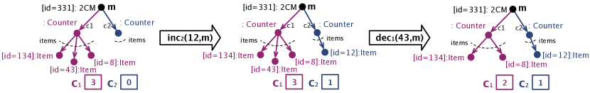
Figure 4: Sample counter manipulation using the BAUML model in Table 2

4.5 Cardinality-Bounded Models

The source of undecidability in Theorem 4.5 relies in the contains relation of $\mathcal{M}^{*}$ (cf. Table 2), which relates its target role items with an unbounded cardinality. To overcome this issue, we introduce the notion of cardinality-bounded BAUML model. A BAUML model $\mathcal{B}=\langle\mathcal{M},\mathcal{O},\mathcal{S},\mathcal{P}\rangle$ is cardinality-bounded if $\mathcal{B}$ is navigational and each target role in $\mathcal{M}$ has a bounded cardinality, i.e., is associated to a cardinality constraint whose upper bound is numeric. $\mathcal{B}$ is N-cardinality-bounded if the maximum upper bound associated to a target role is $N$. If there exists at least a target role with unbounded cardinality, i.e., associated to a cardinality constraint whose upper bound is $*$, then $\mathcal{B}$ is instead said to be cardinality-unbounded. Notice that no cardinality restriction is imposed, for cardinality-bounded models, on the cardinalities associated to roles that are not target roles.

With all these notions at hand, we are now able to state the main result of this paper.

Theorem 4.7.

Let $\mathcal{B}$ be an arbitrary unidirectional, cardinality-bounded BAUML model. Verifying whether $\mathcal{B}$ satisfies a $\mu\mathcal{L}_{p}$ property navigationally compatible with $\mathcal{B}$ is decidable, and reducible to finite-state model checking.

Proof 4.8.

Let $\mathcal{B}=\langle\mathcal{M},\mathcal{O},\mathcal{S},\mathcal{P}\rangle$ be a cardinality-bounded, unidirectional BAUML model, and let $\Phi$ be a $\mu\mathcal{L}_{p}$ property navigationally compatible with $\mathcal{B}$. On the one hand, by inspecting the notion of navigational compatibility, one can notice that $\Phi$ is “rooted” in a single artifact class S, subject to the outermost subformula of the form $\exists x.S(x)\land\Psi(x)$ (or $\forall x.S(x)\rightarrow\Psi(x)$). Navigational compatibility then ensures that $\Phi$ only mentions relations and classes that can be reached by navigating $\mathcal{M}$ using is-a relationships (in both directions), or associations, in a direction that is compatible with the unidirectionality imposed by $\mathcal{B}$.

On the other hand, as pointed out in Section 4.4, in a navigational model like $\mathcal{B}$ it is impossible for artifact instances to share objects that belong to read-write classes. This means that the evolution of an artifact instance is completely independent from that of the other artifact instances of the same type $\textsc{art}_{\texttt{{S}}}$, or other artifact types.

By combining these two observations, we obtain that $\Phi$ obeys to a sort of isolation property:

• $\Phi$ does not distinguish whether the system contains evolving artifact instances of types different than $\textsc{art}_{\texttt{{S}}}$;

• $\Phi$ does not distinguish whether the instances of $\textsc{art}_{\texttt{{S}}}$ evolve in isolation, or co-evolve in a concurrent way.

This isolation property is a data-aware variant of the free-choice property of Petri nets. Thanks to such property, instead of directly considering the whole concurrent evolution of the system, in which unboundedly many artifact instances could be created over time and evolved in parallel, one can consider a faithful, sound and complete abstraction of the system, which accounts only for the concurrent evolution of those instances of type $\textsc{art}_{\texttt{{S}}}$ present in the initial database of $\mathcal{B}$, plus an additional artifact instance of type $\textsc{art}_{\texttt{{S}}}$, nondeterministically created and evolved in addition to the others.

Let $b_{i}$ be the number of artifact instances of type $\textsc{art}_{\texttt{{S}}}$ present in the initial database of the system. From the fact that $\mathcal{B}$ is unidirectional and cardinality-bounded, we have that each artifact instance can create only a bounded amount of objects during its evolution. In fact, the number of objects that can be created by an artifact instance is bounded by $(k\cdot N)^{l+1}$, where: (i) $k$is the number of relations in the schema (which bounds the number of relations that are collectively attached to an artifact/class in the schema), (ii) $N$is the maximum cardinality upper bound attached to a target role belonging to a path rooted in $\textsc{art}_{\texttt{{S}}}$, and (iii) $l$is the length of the longest navigational path rooted in $\textsc{art}_{\texttt{{S}}}$. As a consequence, by considering the aforementioned sound and complete abstraction, we have that at most $(b_{i}+1)\cdot N^{l+1}$ objects and artifact instances are simultaneously present in a system snapshot. The claim then follows by: (i) applying the translation from BAUML models to data-centric dynamic systems (DCDSs) [1], provided in [9]; (ii) observing that the bound $(b_{i}+1)\cdot N^{l+1}$ implies that the obtained DCDSs is state-bounded; (iii) recalling that verification of $\mu\mathcal{L}_{p}$ properties over state-bounded DCDSs is decidable, and reducible to finite-state model checking [1].

An important open point is whether cardinality-boundedness is a sufficient restriction for decidability per sè, i.e., without necessarily imposing unidirectionality. The following theorem provides a strong, negative answer to this question, witnessing that both restrictions are simultaneously required towards decidability.

Theorem 4.9.

Checking termination of 1-cardinality-bounded, bidirectional BAUML models is undecidable.

Proof 4.10.

Given a 2-counter machine $\mathcal{C}$, we produce a corresponding 1-cardinality-bounded, bidirectional BAUML model $\mathcal{B}_{\mathcal{C}}=\langle\mathcal{M}^{b},\emptyset,\{S_{\texttt{2CM}}^{b}\},\{P_{init}^{b},P_{run}^{b}\}\rangle$, whose components are illustrated in Table 2. $\mathcal{M}^{b}$ contains a single artifact 2CM, which can be ready or halted, the latter being the termination state ($\textsc{term}_{\texttt{2CM}}=\texttt{Halted2CM}$), as attested by $S_{\texttt{2CM}}^{b}$. When the $\mathsf{init}$ operation is applied, a new instance $m$ of Ready2CM is created, attaching a dedicated item that represents the zero point for both counters.

Intuitively, $m$ mirrors the two counters in $\mathcal{C}$ as follows. Thanks to the fact that $m$ can navigate and manipulate the association hasNext in both directions (i.e., from left to right and from right to left), the length of the right chain from the zero element $m.zero$ corresponds to the value of the first counter, whereas the length of the left chain from the zero element corresponds to the value of the second counter.

The artifact instance $m$ suitably encodes the commands in $\mathcal{C}$ as follows:

• Incrementing the first counter requires to create a new Item, and to put this object between the zero element and the old right-successor of it (cf. $\mathsf{inc}_{1}$, which conveniently exploits notation “@pre” to query the configuration of objects in the last predecessor state). This has the effect of increasing the length of the right chain of one unit. The alternative operation $\mathsf{incZ}_{1}$ handles the special case in which there is no right-successor from the zero element: in this case incrementing the counter just corresponds to add a new item on the right of the zero element.

• Testing whether the first counter is 0 translates into checking whether set $m.zero.r$ is empty, i.e., whether it is true that the zero element does not have any right successor.

• Decrementing the first counter translates into the removal of one item from set right chain of the zero element. There are two possible cases. In the first case, there is just a single right-successor, i.e., the counter has value 1. In this case, operation $\mathsf{decS_{1}}$ just ensures that $m.zero.r$ does not have anymore this successor. If instead the right chain is longer than 1, then the decrement is handled by making the second right-successor of $m.zero$ the new direct right-successor of it, at the same time isolating the old direct right-successor.

Table 3 shows how these three aspects can be formalized in terms of activity diagrams and OCL queries. The management of the second counter is analogous, with the only difference that it navigates the left chain of the zero element, i.e., it exploits the $l$ role of relation hasNext in place of the $r$ role. Figure 4 intuitively shows the evolution of a specific configuration of the system in response to the application of two operations.

Observe that, as clearly shown by $\mathcal{M}^{b}$, $\mathcal{B}_{\mathcal{C}}$ is 1-cardinality-bounded, and is bidirectional, because relation hasNext is navigated on both directions, making both $l$ and $r$ target roles. Furthermore, like for the reduction in Theorem 4.5, each artifact instance is created in state Ready2CM, and evolves completely independently from the other artifact instances. This means that either all instances of Ready2CM halt, or none halt. The claim follows by observing that $\mathcal{C}$ halts if and only if all instances of Ready2CM eventually reach the $\mathsf{Halted2CM}$ state, i.e., properly terminate.

$\mathcal{M}^{b}$	$S_{\texttt{2CM}}^{b}$

$P_{init}^{b}$		$\mathsf{init}\ \begin{array}[t]{@{}l@{\ }l}\textbf{pre:}&\neg(\texttt{Ready2CM}.allInstances()\rightarrow exists(m^{\prime}|m^{\prime}.id=id))\\ \textbf{post:}&\mathit{\texttt{Ready2CM}.allInstances()\rightarrow exists(m|\begin{array}[t]{@{}l}m.oclIsNew()\land{}m.id=id\land result=m\\ \land m.zero\rightarrow exists(i|i.oclIsNew())~{})\end{array}}\\ \end{array}$

$P_{run}^{b}$	start
	$k:\mathsf{INC}(1,k^{\prime})$		$\begin{array}[]{@{}l}Q_{0}^{1}=(\mathit{m.zero.r\rightarrow isEmpty()})\\[6.0pt] \begin{array}[]{@{}ll@{\ }l}\mathsf{incZ_{1}}&\textbf{post:}&\mathit{m.zero.r\rightarrow exists(i|i.oclIsNew())}\\ \mathsf{inc_{1}}&\textbf{post:}&\mathit{m.zero.r\rightarrow exists(i|}\begin{array}[t]{@{}l}\mathit{i.oclIsNew()}\\ \mathit{\land i.r=m.zero.r@pre)}\end{array}\end{array}\end{array}$
	$k:\mathsf{CDEC}(1,k^{\prime},k^{\prime\prime})$		$\begin{array}[]{@{}l}Q_{0}^{1}=(\mathit{m.zero.r\rightarrow isEmpty()})\quad Q_{1}^{1}=(\mathit{m.zero.r.r\rightarrow isEmpty()})\\[6.0pt] \begin{array}[]{@{}ll@{\ }l}\mathsf{decS_{1}}&\textbf{post:}&\mathit{m.zero.r\rightarrow isEmpty()}\\ \mathsf{dec_{1}}&\textbf{post:}&\text{let }\mathit{old_{r}=m.zero.r@pre,new_{r}=m.zero.r.r@pre}\\ &&\text{in }\mathit{m.zero.r=new_{r}\land(old_{r}.r\rightarrow isEmpty())}\end{array}\end{array}$
	$n:\mathsf{HALT}$		$\mathsf{halt}\ \begin{array}[t]{@{}l@{\ }l}\textbf{post:}&\mathit{\neg(m.oclIsTypeOf(\texttt{Ready2CM}))}\\ &\mathit{\land m.oclIsTypeOf(\texttt{Halted2CM})}\end{array}$

Table 3: 1-cardinality-bounded, bidirectional BAUML model simulating a 2-counter machine

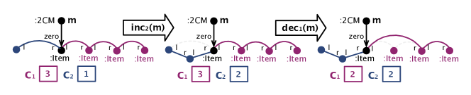
Figure 5: Sample counter manipulation using the BAUML model in Table 3

$\mathcal{M}^{bu}$	$S_{\texttt{Conn}}$

$P_{init}^{bu}$		$\begin{array}[]{@{}l}\begin{array}[]{@{}l@{\ }l}Q_{PC}&=\mathit{\texttt{PC}.allInstances()\rightarrow isEmpty()}\\ Q_{I}&=\mathit{\texttt{Item}.allInstances()\rightarrow isEmpty()}\\[6.0pt] \end{array}\\ \begin{array}[t]{@{}l@{\ }l@{\ }l}\mathsf{createPC}&\textbf{post:}&\mathit{\texttt{PC}.allInstances()\rightarrow exists(pc|pc.oclIsNew()\land pc.pos=\mathsf{1}))}\\ \mathsf{init}&\textbf{pre:}&\neg(\texttt{ReadyConn}.allInstances()\rightarrow exists(m^{\prime}|m^{\prime}.id=id))\\ &\textbf{post:}&\mathit{\texttt{ReadyConn}.allInstances()\rightarrow exists(c|\begin{array}[t]{@{}l}c.oclIsNew()\land c.id=id\land result=c\\ \land c.pc=(\texttt{PC}.allInstances()))\end{array}}\\ \mathsf{attach}&\textbf{post:}&\mathit{c.r\rightarrow exists(s_{1}|s_{1}.oclIsNew()\land s_{1}.lastR=\mathsf{true}\land s_{1}.startC1=\mathsf{true})}\\ &&\mathit{\land c.l\rightarrow exists(s_{2}|s_{2}.oclIsNew()\land s_{2}.lastL=\mathsf{true}\land s_{2}.startC2=\mathsf{true})}\end{array}\end{array}$

$P_{run}^{bu}$	start
	$k:\mathsf{INC}(1,k^{\prime})$		$\begin{array}[]{@{}l}\begin{array}[]{@{}l@{\ }c@{\ }l}Q_{+}&=&\mathit{(c.pc=\mathsf{k})\land(c.l\rightarrow isEmtpy())\land(c.r\rightarrow isEmpty())}\\ Q_{loop}&=&\mathit{(c.pc=\mathsf{k})\land\neg((c.l\rightarrow isEmtpy())\land(c.r\rightarrow isEmpty()))}\\ Q_{fw}^{\mathsf{k^{\prime}_{i}}}&=&(\mathit{c.pc=\mathsf{k^{\prime}_{i}}})\text{ for }\mathsf{k^{\prime}_{i}}\in\{\mathsf{1},\ldots,\mathsf{n}\}\setminus\{\mathsf{k},\mathsf{k^{\prime}}\}\end{array}\\[6.0pt] \begin{array}[t]{@{}l@{\ }l@{\ }l}\mathsf{\mathsf{k}Inc_{1}}&\textbf{post:}&\text{let }\mathit{i=(\texttt{Item}.allInstances()\rightarrow select(i^{\prime}|i^{\prime}.lastR))}\\ &&\text{in }\mathit{c.l=i\land i.lastR=\mathsf{false}}\\ &&\phantom{\text{in }}\mathit{\land c.r\rightarrow exists(i^{\prime\prime}|i^{\prime\prime}.isOclNew()\land i^{\prime\prime}.lastR=\mathsf{true})}\\ &&\phantom{\text{in }}\mathit{\land c.pc=\mathsf{k^{\prime}}}\\ \end{array}\end{array}$
	$k:\mathsf{CDEC}(1,k^{\prime},k^{\prime\prime})$		$\begin{array}[]{@{}l}\begin{array}[]{@{}l@{\ }c@{\ }l}Q_{0}^{1}&=&\mathit{(c.pc=\mathsf{k})\land c.r.lastR\land c.r.startC1}\\ Q_{-}^{1}&=&\mathit{(c.pc=\mathsf{k})\land c.r.lastR\land\neg c.r.startC1}\\ Q_{loop}&=&\mathit{(c.pc=\mathsf{k})\land\neg c.r.lastR}\\ Q_{fw}^{\mathsf{k^{\prime}_{i}}}&=&(\mathit{c.pc=\mathsf{k^{\prime}_{i}}})\text{ for }\mathsf{k^{\prime}_{i}}\in\{\mathsf{1},\ldots,\mathsf{n}\}\setminus\{\mathsf{k},\mathsf{k^{\prime}},\mathsf{k^{\prime\prime}}\}\\[6.0pt] \end{array}\\ \begin{array}[t]{@{}ll@{\ }l}\mathsf{\mathsf{k}PC}&\textbf{post:}&\mathit{c.pc=\mathsf{k^{\prime\prime}}}\\ \mathsf{kDec_{1}}&\textbf{post:}&\text{let }\mathit{i_{r}=c.r@pre,i_{l}=c.l@pre}\\ &&\text{in }\mathit{i_{l}.lastR=\mathsf{true}\land i_{r}.lastR=\mathsf{false}}\\ &&\phantom{\text{in }}\mathit{\land(c.l\rightarrow isEmpty())\land(c.r.\rightarrow isEmpty())}\end{array}\end{array}$
	$n:\mathsf{HALT}$		$\mathsf{halt}\ \begin{array}[t]{@{}l@{\ }l}\textbf{post:}&\mathit{\neg(m.oclIsTypeOf(\texttt{ReadyConn}))}\\ &\mathit{\land m.oclIsTypeOf(\texttt{HaltedConn})}\end{array}$

Table 4: 1-cardinality-bounded, unidirectional BAUML model with shared objects simulating a 2-counter machine

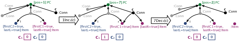
Figure 6: Sample counter manipulation using the BAUML model in Table 4

4.6 Models With Shared Instances

As argued in Section 4.4, unidirectional BAUML models are not able to make artifact instances share (read-write) objects. In this section, we study what happens if we relax unidirectionality so as to support this feature. A unidirectional BAUML model with shared instances $\mathcal{B}=\langle\mathcal{M},\mathcal{O},\mathcal{S},\mathcal{P}\rangle$ is a BAUML model in which, inside navigational expressions, it is possible to add free queries over $\mathcal{M}_{rw}$, provided that they do not contain the expression $\mathit{oclIsNew()}$. Intuitively, this means that new objects can only be created through standard navigational OCL expressions, but at the same time it is possible to establish associations with already existing objects that are not reachable by simply navigating from the artifact instance. The following theorem shows that this relaxation makes verification again undecidable.

Theorem 4.11.

Checking termination of 1-cardinality-bounded, unidirectional BAUML models with shared instances is undecidable.

Proof 4.12.

Given a 2-counter machine $\mathcal{C}$, we produce a corresponding 1-cardinality-bounded unidirectional BAUML model with shared instances $\mathcal{B}_{\mathcal{C}}=\langle\mathcal{M}^{bu},\emptyset,\{S_{\texttt{2CM}}^{bu}\},\{P_{init}^{bu},P_{run}^{bu}\}\rangle$, whose components are illustrated in Table 4.

As shown in Table 4, $\mathcal{M}^{bu}$ contains a single artifact Conn, which can be ready or halted, the latter being the termination state ($\textsc{term}_{\texttt{Conn}}=\texttt{HaltedConn}$), as attested by $S_{\texttt{Conn}}^{bu}$. Due to cardinality boundedness and unidirectionality, a single instance of $\mathcal{B}_{\mathcal{C}}$ is not powerful enough to simulate $\mathcal{C}$. Hence, differently from the previous undecidability proofs, the two counters are now simulated by unbouded chains of artifact instances. In this light, the main difficulty is to properly “synchronize” such different instances so as to ensure that they collectively implement the program of $\mathcal{C}$, without interfering with each other. To realize such a synchronization, all instances of Conn share an instance of PC, which represents a “program counter” to keep track of the current instruction to be processed in $\mathcal{C}$. Intuitively, each instance of Conn represents a connection between two items; a chain of three items is then built by using two instances of Conn, making sure that the first instance has on the right the same Item that the second instance has on the left. This structure constitutes the basis for simulating a counter.

Let us now go into the details of such a simulation. The initialization transition in $S_{\texttt{Conn}}^{bu}$ consists now of a complex activity diagram $P_{init}^{bu}$, which consists of the following steps:

• Initially, if there is no instance of the program counter, one instance is created, setting its “position” (represented by a string attribute pos) to the constant string $\mathsf{1}$. If an instance of PC already exists, then this step is skipped.

• The second step consists of the creation of a new connection artifact instance (of type Conn), with a distinguished identifier. Upon creation, the $pc$ role of this connection points to the only available instance of PC.

• The third steps is applied only if no instance of class Item exists in the system. In this case, two special items are created so as to represent the zero elements for the two counters of $\mathcal{C}$. This is done as follows:

  • The zero element for the first counter consists of a newly created instance $i_{0}^{R}$ of Item, whose boolean attribute $startC1$ is set to $\mathsf{true}$. Item $i_{0}^{R}$ is attached to the right of the just created instance of Conn. Since $i_{0}^{R}$ is not on the left of any connection, also its boolean attribute $lastR$ is set to $\mathsf{true}$.

  • The zero element for the second counter consists of a newly created instance $i_{0}^{L}$ of Item, whose boolean attribute $startC2$ is set to $\mathsf{true}$. Item $i_{0}^{L}$ is attached to the left of the just created instance of Conn. Since $i_{0}^{L}$ is not on the right of any connection, also its boolean attribute $lastL$ is set to $\mathsf{true}$.

The structure obtained when $4$ instances of $P_{init}^{bu}$ are executed in a row can be seen on the left of Figure 6.

The idea behind the manipulation of counters starting from this structure is to extend (resp., reduce) the chain on the right of item $i_{0}^{R}$ to increment (resp., decrement) the first counter, and to extend (resp., reduce) the chain on the left of item $i_{0}^{R}$ to increment (resp., decrement) the second counter. Since the case of the second counter is obtained by just mirroring that of the first counter, we just concentrate on the first counter.

The first important observation, which is common to the case of counter increment and decrement, concerns the problem of synchronization. On the one hand, as already pointed out we want all instances of Conn to collectively realize the program of $\mathcal{C}$. On the other hand, there is no control on when new instances of Conn are created. In particular, it could be the case that a new connection is created when the other active connections have already executed part of the program of $\mathcal{C}$. Similarly, since there is no control on how the different active instances of Conn interleave with each other, when a connection executes the portion of $P_{run}^{bu}$ corresponding to instruction number $k$ in $\mathcal{C}$, it must ensure that $k$ is indeed the current intruction. More specifically, instruction number $k$ always contains an initial choice, used to check whether the program counter is indeed $k$ and, if so, whether the instance of Conn that is executing the process is responsible for the execution of instruction $k$, or should instead just execute an “idle” loop and wait that the responsible connection executes step $k$. If the program counter stores in its $pos$ attribute an instruction identifier different than $k$, then the process just “jumps” to the right step. If instead the program counter corresponds to $k$, then a different behavior is exhibited depending on whether the instruction number $k$ corresponds to an increment or conditional decrement for the first counter.

In the case of increment:

• If the connection is not associated to any item on its left and its right (i.e., it is not part of any chain), then the connection becomes responsible for the increment, which is atomically executed using the operation $\textbf{k}Inc_{1}$. The increment is realized as follows:

  • The unique item (called $i$) that has attribute $lastR$ set to $\mathsf{true}$ is selected.

  • This item is attached on the left of the current connection, setting its $lastR$ attribute to $\mathsf{false}$. In this way, it is easy to see that an item has $lastR=\mathsf{false}$ if and only if there is no connection that has it on the left.

  • A new item is created and attached on the right of the current connection, setting its $lastR$ attribute to $\mathsf{true}$. This newly created item represents the increment of the first counter, and the current connection acts as the last connection of the chain simulating the first counter.

  • The program counter is updated, setting its $pos$ attribute to the string that corresponds to the new instruction identifier $k^{\prime}$. Since $k^{\prime}$ is a pre-defined string, each increment is different from the others, and this is why each specific increment is mapped to a separate operation in $P_{run}^{bu}$.

  Considering e.g., the case of instruction $1:\mathsf{INC}(1,7)$, the central part of Figure 6 represents the new data configuration after the execution of this step by one of the connections that are currently active but not associated to any item.

• If instead the connection is already attached to an item on the left or on the right, then it executes an idle step, going back to check whether the program counter is still $k$ or has instead been updated.

In the case of conditional decrement:

• If the connection has on its right an item whose attribute $lastR$ is $\mathsf{true}$, then the connection becomes responsible for the conditional decrement. Two cases may then arise: either the first counter is 0, and consequently only the program counter must be updated, or the counter is positive, and consequently the counter must be decremented before updating the program counter. The test for zero can be easily captured in $\mathcal{B}^{bu}$ by testing whether the item having $lastR=\mathsf{true}$ also has $startC1=\mathsf{true}$: if so, then the first counter is zero, if not, then the first counter is positive. In the former case, captured by query $Q^{1}_{0}$, the specific task $\textbf{k}PC$ is executed, whose effect is simply to update the attribute $pos$ of the program counter to the string corresponding to $k^{\prime\prime}$; since $k^{\prime\prime}$ is a pre-defined string, each program counter update is different from the others, and this is why each specific program counter update is mapped to a separate operation in $P_{run}^{bu}$. In the latter case, captured by query $Q^{1}_{-}$, an atomic decrement and program counter update is executed using the operation $\textbf{k}Dec_{1}$. The decrement is realized as follows:

  • The item that was previously on the right of the connection is updated making its $lastR$ attribute equal to $\mathsf{false}$.

  • The item that was previously on the left of the connection (i.e., on the right of the previous connection along the chain) is updated making its $lastR$ attribute equal to $\mathsf{true}$.

  • The connection is disconnected from both such items, hence reducing the chain of one item. This has also the indirect effect of making the connection eligible for being responsible of a successive increment.

  • The program counter is updated, setting its $pos$ attribute to the string that corresponds to the new instruction identifier $k^{\prime}$. Since $k^{\prime}$ is a pre-defined string, each decrement is different from the others, and this is why each specific decrement is mapped to a separate operation in $P_{run}^{bu}$.

  Considering the case of instruction $7:\mathsf{CDEC}(1,2,9)$, the right part of Figure 6 represents the new data configuration after the execution of this step by the connection that is currently at the end of the right chain.

• If instead the connection does not have on its right the element whose $lastR$ attribute is $\mathsf{true}$, then it executes an idle step, going back to check whether the program counter is still $k$ or has instead been updated.

As soon as one of the active connection artifact instances sets the program counter to the constant $\mathsf{n}$, all active connections move to the final part of $P_{run}^{bu}$, where they are moved from the ReadyConn to the HaltedConn state. If new instances of Conn are subsequently created, they immediately jump to execute this task as well (in fact, they all share the same program counter, whose $pos$ attribute continues to be $\mathsf{n}$). This means that either all instances of ReadyConn halt, or none halts. The claim follows by observing that $\mathcal{C}$ halts if and only if all instances of ReadyConn eventually reach the $\mathsf{HaltedConn}$ state, i.e., properly terminate.

We close this thorough analysis by showing that, if we introduce a bound on the number of artifact instances that are simultaneously active in the system, verification becomes decidable for this specific class of BAUML models. This technique cannot be applied to unrestricted nor unbounded BAUML models: by inspecting the proofs of Theorems 4.3 and 4.5, one can easily notice that undecidability holds even when there is just a single active artifact instance.

Theorem 4.13.

Verification of $\mu\mathcal{L}_{p}$ properties over cardinality-bounded, unidirectional BAUML models with shared instances of read-write classes is decidable and reducible to finite-state model checking when the number of simultaneously active artifact instances is bounded.

Proof 4.14.

Let $\mathcal{B}$ be a cardinality-bounded, unidirectional BAUML model. By combining unidirectionality and cardinality-boundedness, we have that an artifact instance can create only a bounded amount of objects during its evolution. In fact, the number of objects that can be created is bounded by $(k\cdot N)^{l+1}$, where $k$, $N$ and $l$ are as in the proof of Theorem 4.7. Since the number of simultaneously active artifact instances is bounded, say, by a number $b$, then at each time point the number of objects and artifact instances present in the overall system is bounded by $b\cdot(k\cdot N)^{l+1}$. The claim then follows by: (i) applying the translation from BAUML models to DCDSs, described in [9]; (ii) observing that the bound $b\cdot(k\cdot N)^{l+1}$ implies that the obtained DCDS is state-bounded; (iii) recalling that verification of $\mu\mathcal{L}_{p}$ properties over state-bounded DCDSs is decidable, and reducible to finite-state model checking [1].

It is important to observe that bounding the number of simultaneously active artifact instances still allows one to create an unbounded amount of artifact instances over time, provided that they do not accumulate in the same snapshot. In this light, Theorem 4.13 closely resembles the result given in [20] for business artifacts specified in the GSM notation.

To show the practical relevance of these results, we return to our example, presented in Section 3. It is a realistic example of a data-centric business process. At the same time it is a cardinality-bounded, unidirectional model with shared instances coming from a read-only relation (ItemType). Hence, it falls into the case of Theorem 4.7, for which verification is decidable even in presence of unboundedly many simultaneously active artifact instances. In the case where artifacts share a read-write relation, decidability requires an additional bound on the number of simultaneously active artifact instances, so as to fall into Theorem 4.13.

5 Related Work

This section will examine alternative representations for artifact-centric business process models, with the focus on the data dimension. In those cases where it is possible, we will review the decidability results that have been obtained for the formal verification of these models. However, most of these results are applicable to models grounded on logic or mathematical notations that do not provide a practical business level representation. We will first begin by looking at alternative graphical representations and we will continue with alternatives grounded on logic.

Apart from the work in [8] that we have considered in this paper, there are also other approaches that use UML class diagrams to represent the data dimension, such as [10]. However, [10] turns to proclets (a labeled Petri net with ports) to represent the internal lifecycle of the artifact and how it relates to other artifacts.

ER models [4] are similar to UML class diagrams as they also allow representing the relationships between the artifacts and their attributes. The PHILharmonic Flows framework [16] represents business processes with data in a graphical way, using a model which falls in-between a UML diagram and a database schema representation. Unlike our approach, it does not distinguish between what we call business artifacts and objects.

Another alternative is to extend BPMN to allow the representation of data-dependencies in the business process model [17]. However, [17] does not have a specific diagram showing the relationships between the data or artifacts. The Guard-Stage-Milestone (GSM) approach [14, 7] represents the artifact and its lifecycle in one model, which shows the guards, stages and milestones involved in the evolution of an artifact. In contrast to the UML class diagram, GSM does not show graphically the relationships between the artifacts: they are encoded as attributes instead.

Several works deal with the formal verification of GSM models and study their decidability. For instance, [20] uses an approach that is very close to ours. It relies on the notion of state-boundedness to guarantee decidability. Similarly, [3] deals with decidability of GSM models but taking agents (i.e. users or automatic systems) into consideration. [12] also applies model checking to these models, but its implementation restricts the data types and only admits one artifact instance. Both [3] and [12] use CTL or a variant of CTL, neither of which are as powerful as $\mu$-calculus.

There are several works [1, 2, 5] that deal with verification of artifact-centric business process models represented by means of a data-centric dynamic system (DCDS). DCDSs are grounded on logic. [1] represents artifacts by means of a relational database schema, [2] uses a knowledge and action base defined in a variant of Description Logics, and [5] maps an ontology to a DCDS. All these works define the properties to be checked in variants of $\mu$-calculus. They ensure decidability either by state-boundedness [1, 5] or by limiting the calls to functions that obtain new values [2, 1].

Works such as [6] and [11] also verify the fulfillment of properties by the model but they both define properties in variants of LTL or CTL (respectively), making them less powerful than $\mu$-calculus. [6] represents the data by means of a database schema. It allows the use of integrity constraints in the data and arithmetic operations, requiring the condition of feedback-freedom (i.e. output variables cannot be reused from one function to the next) to guarantee decidability. [11] opts for bounding the domain values or to limit the language that is used instead. Artifacts are represented by means of a tuple which includes a set of attributes.

6 Conclusions

We have analyzed the decidability of verification for artifact-centric business process models defined according to the BALSA framework and at a high level of abstraction. That is, we have lifted the decidability conditions from the formal, low-level representations, to the business level, to establish conditions which can be considered by the modeler of the process. Although we have focused on the representation of these elements using UML, our results could be extended to other forms of representation.

As a result of our analysis, we have concluded that verification of artifact-centric process models is only decidable when: (i) artifacts are linked to a bounded number of objects, (ii) two different artifacts only share read-only objects, (iii) expressions in the pre and postconditions of the operations are navigational starting from the artifact instance being manipulated, and (iv) the associations specified among two classes are not navigated back and forth. If any of these four conditions is relaxed, then we end-up with undecidability. Regaining decidability when the model contains shared read-write objects requires to put a bound on the number of simulatenously active artifact instances. Although these conditions are restrictive, they still allow for the definition of relevant situations in practice.

As further work, we would like to pursue this line of research so as to characterize concrete, real-life settings for which decidability of verification is guaranteed. We also plan to provide a more fine-grained characterization of how read and write operations might interact without undermining decidability. Finally, we aim at studying the practical applicability of our verification techniques, by understanding how the exponentiality in the data that is inherent in data-aware systems can be tamed, through a suitable modularization/partitioning of the data into independent portions.

References

- [1] B. Bagheri Hariri, D. Calvanese, G. D. Giacomo, A. Deutsch, and M. Montali. Verification of relational data-centric dynamic systems with external services. In Proc. of PODS, pages 163–174. ACM, 2013.
- [2] B. Bagheri Hariri, D. Calvanese, M. Montali, G. De Giacomo, R. De Masellis, and P. Felli. Description logic knowledge and action bases. J. Artif. Intell. Res., 46:651–686, 2013.
- [3] F. Belardinelli, A. Lomuscio, and F. Patrizi. Verification of GSM-based artifact-centric systems through finite abstraction. In Proc. of ICSOC, volume 7636 of LNCS, pages 17–31. Springer, 2012.
- [4] K. Bhattacharya, R. Hull, and J. Su. A data-centric design methodology for business processes. In Handbook of Research on Business Process Management, pages 1–28. 2009.
- [5] D. Calvanese, G. D. Giacomo, D. Lembo, M. Montali, and A. Santoso. Ontology-based governance of data-aware processes. In Proc. of RR, volume 7497 of LNCS, pages 25–41. Springer, 2012.
- [6] E. Damaggio, A. Deutsch, and V. Vianu. Artifact systems with data dependencies and arithmetic. ACM Trans. on Database Systems, 37(3):1–36, Aug. 2012.
- [7] E. Damaggio, R. Hull, and R. Vaculín. On the equivalence of incremental and fixpoint semantics for business artifacts with guard-stage-milestone lifecycles. Inf. Syst., 38(4):561–584, 2013.
- [8] M. Estañol, A. Queralt, M.-R. Sancho, and E. Teniente. Artifact-centric business process models in UML. In Proc. of BPM Workshops, volume 132 of LNBIP, pages 292–303. Springer, 2012.
- [9] M. Estañol, M.-R. Sancho, and E. Teniente. Reasoning on UML data-centric business process models. In Proc. of ICSOC, volume 8274 of LNCS, pages 437–445. Springer, 2013.
- [10] D. Fahland, M. D. Leoni, B. F. van Dongen, and W. M. P. van der Aalst. Behavioral conformance of artifact-centric process models. In Proc. of BIS, volume 87 of LNBIP, pages 37–49. Springer, 2011.
- [11] C. E. Gerede and J. Su. Specification and verification of artifact behaviors in business process models. In Proc. of ICSOC, volume 4749 of LNCS, pages 181–192. Springer, 2007.
- [12] P. Gonzalez, A. Griesmayer, and A. Lomuscio. Verifying GSM-based business artifacts. In Proc. of ICWS, pages 25–32. IEEE, 2012.
- [13] R. Hull. Artifact-centric business process models: Brief survey of research results and challenges. In Proc. of OTM, volume 5332 of LNCS, pages 1152–1163. Springer, 2008.
- [14] R. Hull et al. Business artifacts with guard-stage-milestone lifecycles: managing artifact interactions with conditions and events. In Proc. of DEBS, pages 51–62. ACM, 2011.
- [15] ISO. ISO/IEC 19505-2:2012 - OMG UML superstructure 2.4.1. Technical Report ISO/IEC 19505-2:2012, OMG, 2012.
- [16] V. Künzle and M. Reichert. PHILharmonicFlows: towards a framework for object-aware process management. Software Maintenance, 23(4), 2011.
- [17] A. Meyer, L. Pufahl, D. Fahland, and M. Weske. Modeling and enacting complex data dependencies in business processes. In Proc. of BPM, volume 8094 of LNCS, pages 171–186. Springer, 2013.
- [18] M. L. Minsky. Computation: Finite and Infinite Machines. Prentice-Hall, 1967.
- [19] OMG. OCL version 2.4. Technical report, OMG, 2014.
- [20] D. Solomakhin, M. Montali, S. Tessaris, and R. D. Masellis. Verification of artifact-centric systems: Decidability and modeling issues. In Proc. of ICSOC, volume 8274 of LNCS, pages 252–266. Springer, 2013.
- [21] M. Weske. Business Process Management: Concepts, Languages, Architectures. Springer, 2007.