The chiral phase transition in two-flavor QCD from imaginary chemical potential

Abstract

We investigate the order of the finite temperature chiral symmetry restoration transition for QCD with two massless fermions, by using a novel method, based on simulating imaginary values of the quark chemical potential $\mu=i\mu_{i},\mu_{i}\in\mathbb{R}$. Our method exploits the fact that, for low enough quark mass $m$ and large enough chemical potential $\mu_{i}$, the chiral transition is decidedly first order, then turning into crossover at a critical mass $m_{c}(\mu)$. It is thus possible to determine the critical line in the $m-\mu^{2}$ plane, which can be safely extrapolated to the chiral limit by taking advantage of the known tricritical indices governing its shape. We test this method with standard staggered fermions and the result of our simulations is that $m_{c}(\mu=0)$ is positive, so that the phase transition at zero density is definitely first order in the chiral limit, on our coarse $N_{t}=4$ lattices with $a\simeq 0.3\,\mathrm{fm}$.

I Introduction

Quantum Chromodynamics is known to undergo a finite temperature “transition” at which both partial deconfinement and partial chiral symmetry restoration take place. Because of its relevance to heavy ion collisions, the early universe and astrophysics, the nature of this QCD transition is the subject of intense numerical studies. Present results show the absence of a true non-analytic phase transition in the case of physical quark masses nature ; tchot ; tchot2 , so that deconfinement would just correspond to a rapid analytic change of the effective degrees of freedom (crossover). This is consistent with the fact that the global symmetries of QCD associated with the transition are only exact in the limits of infinite quark masses (center symmetry) or of massless quarks (chiral symmetry): only in these limits is a true phase transition expected a priori, representing a change in the realization of the corresponding symmetry.

However, a full understanding of the QCD phase diagram, and in particular of the interplay between center symmetry and chiral symmetry, requires to study the phase transition as a function of the quark masses. The current state of knowledge at zero baryon density is summarized in Fig. 1. For three degenerate flavors, QCD displays a first order phase transition in the limits of zero and infinite quark masses, associated with the breaking of the chiral and center symmetries, respectively. For finite quark masses, instead, these symmetries are broken explicitly; the associated first order transitions weaken away from these limits, until they disappear at critical points, belonging to the Ising ($Z_{2}$) universality class. The chiral chcrit ; mu4 and deconfinement deccrit ; saito ; saito1 critical lines are known on coarse $N_{t}=4$ lattices, based on simulations with staggered and Wilson fermions, respectively.

Figure 1: Schematic behavior of the order of the finite temperature phase transition for $N_{f}=2+1$ QCD as a function of the up/down and strange quark masses $(m_{u,d},m_{s})$, at zero baryon chemical potential. $O(4)$ and $Z_{2}$ denote transitions of the second order in the universality class of the $3d$ $O(4)$ and Ising models, respectively.

A still open issue is the order of the transition in the limit of two massless flavors (upper left corner of Fig. 1). This is in fact a longstanding problem, with a history of conflicting lattice results between Wilson Tsukuba ; cp-pacs and staggered, and even within staggered fuku1 ; fuku2 ; columbia ; karsch1 ; karsch2 ; jlqcd ; milc ; DiG ; Unger fermions. The possibilities for continuum QCD have been discussed systematically in Refs. pw ; vicari ; vicari2 . The classical action has a global $SU(2)_{R}\times SU(2)_{L}\times U_{A}(1)$ chiral symmetry, with the $U_{A}(1)$ undergoing anomalous breaking and expected to be effectively restored at high temperature. Since the phase transition is associated with a change in the realization of an exact symmetry, an analytic crossover is ruled out, leaving room for either a first order or second order transition. In the case of a second order transition, the corresponding universality class is fixed by the critical behavior of the associated effective chiral model: that can be $SU(2)_{L}\times SU(2)_{R}\simeq O(4)$, or $U(2)_{R}\times U(2)_{L}/U(2)_{V}$ vicari ; vicari2 , depending on the strength of the axial anomaly at the transition temperature. A first order transition, instead, can be present independently of the critical behavior of the chiral effective model, though it is generally believed that a vanishing strength of the axial anomaly could make it more likely pw ; vicari ; mehta ; vicari2 . In fact, the presence or absence of a first order transition is something which depends on the interplay among the degrees of freedom of the strong interactions which are effective around the transition, and can be decided only on the basis of direct numerical simulations of QCD. Once finite quark masses are switched on, a second order transition disappears immediately, while a first order transition gets gradually weakened, until it disappears at a $Z_{2}$ critical point. The two possible cases are sketched in Fig. 2.

Unfortunately, distinguishing between these two scenarios (first or second order transition) by lattice simulations is notoriously difficult. Since massless fermions cannot be directly simulated, the standard strategy is to perform simulations at a number of finite quark masses, trying to approach the chiral limit. If the transition is second order, then one should observe the scaling relations expected near the critical point. If the transition is first order, one possibility is to directly detect the first order line at finite quark mass, by observing the associated discontinuities and metastabilities. Alternatively, if the critical quark mass $m_{c}$ at which the first order disappears is too small to be probed directly, one should look for the $Z_{2}$ critical behavior near the critical endpoint.

Various studies have found no signs of metatabilities in the range of masses explored up to now, thus failing a direct detection of first order. On the other hand, as we discuss in the following, the analysis of the critical behavior is still not conclusive. Most scaling relations are given in terms of the symmetry breaking parameter, i.e. the quark mass $m$. Examples are given by the divergent part of the susceptibility of the order parameter (i.e. the chiral susceptibility):

$$\chi(m)\sim B\,m^{(1-\delta)/\delta}\;$$ (1)

or, alternatively, by the pseudo-critical temperature as a function of the quark mass:

$$T_{c}(m)=T_{c}(0)+A\,m^{1/(\beta\delta)}\;.$$ (2)

Figure 2: Possible scenarios for the chiral phase transition as function of the pion mass.

Unfortunately, the critical behavior turns out to be very similar for the various universality classes which could be relevant. For instance, the behavior of the chiral susceptibility turns out to be consistent with the $O(4)$ scenario ($1-1/\delta\simeq 0.79$, see O4a ; O4b ), but it is hardly possible to distinguish it from that predicted by the $U(2)_{R}\times U(2)_{L}/U(2)_{V}$ universality class (whose critical indices are almost identical to that of the $O(4)$ case, see vicari2 ), from other $O(N)$ universality classes (e.g $O(2)$, see O2 ), or even from the $Z_{2}$ critical behavior associated with a critical endpoint mass $m_{c}$ close to zero ($1-1/\delta\simeq 0.79$ for $Z_{2}$, see Z2 ).

The same is true for the behavior of the pseudocritical temperature, as noted both for staggered DiG and Wilson tmft fermions, since the critical exponents are very close, e.g. $1/(\beta\delta)\simeq 0.537,0.639$ for $O(4),Z_{2}$, respectively (see O4a ; O4b ; Z2 ), so that there is no way of distinguishing the correct scenario within the range of currently explorable quark masses. A more sensitive quantity would be the specific heat DiG , whose critical exponent is $\alpha\simeq-0.24,0.11,1$ for $O(4)$, $Z_{2}$ and first order respectively (see O4a ; O4b ; Z2 ), but unfortunately determining $\alpha$ by lattice simulations is made difficult by the presence of large non-singular contributions.

In the present paper, we propose an alternative approach to solve this problem, which is based on the investigation of the phase diagram in the presence of a purely imaginary quark chemical potential $\mu=i\mu_{i}$. This is usually exploited to partially circumvent, via analytic continuation, the sign problem which is met in QCD at finite baryon density. However, the phase diagram at imaginary $\mu$ turns out to be quite interesting by itself and, by exploiting its peculiar features, we can extract useful information for the problem at hand.

Our approach is based on the clear evidence of the first order nature of the transition at large enough imaginary chemical potentials and low quark masses. The nature of the transition in the chiral limit can be explored by determining the maximal quark mass necessary to keep the transition first order while driving the chemical potential to zero. While answering this question might appear as difficult as (or even harder than) the original problem, the issue is greatly simplified by taking advantage of the universal tricritical scaling, which imposes strong constraints on the boundary of the first order region, as discussed below.

The paper is organized as follows. In Sec. II we discuss the general form of the QCD phase diagram at imaginary chemical potential. Some of its properties are used in Sec. III to propose our new method to assess the problem of the determination of the order of the $N_{f}=2$ chiral transition at $\mu=0$. In Sec. IV we describe our numerical setting and the results obtained by using the introduced method. Finally in Sec. V we present our conclusions and perspectives for future studies. Preliminary results have been presented in pos .

II Phase diagram for imaginary chemical potential

Figure 3: Generic phase diagram as a function of imaginary chemical potential and temperature. Solid lines are first order Roberge-Weiss transitions. The behavior along dashed lines depends on the number of flavors and the quark masses.

When the chemical potential is considered as a generic complex parameter entering the definition of the partition function $Z$, the two following exact symmetries emerge (RW )

$$Z(\mu)=Z(-\mu),\quad Z\left(\frac{\mu}{T}\right)=Z\left(\frac{\mu}{T}+i\frac{2\pi n}{3}\right)\quad n\in\mathbb{Z}\ ,$$ (3)

which imply reflection symmetry in the imaginary $\mu$ direction about the “Roberge-Weiss” values $\mu=i\pi T/3(2n+1)$. Along these lines a $Z_{2}$ exact symmetry is present RW , which can be explicitly realized or spontaneously broken, different sectors corresponding to different preferred orientations of the Polyakov loop. Transitions between neighboring sectors are of first order for high $T$ RW and analytic crossovers for low $T$ fp1 ; el1 ; ddl . The first order transition lines at $\mu=i\pi T/3(2n+1)$ may end with a second order critical point or with a triple point, branching off into two first order lines. One of these may continue to zero and real chemical potential and represents the analytic continuation of the chiral or deconfinement transition. For the deconfinement transition this has been explicitly demonstrated in deccrit , for the chiral transition it is demonstrated in the present work. Which of these possibilities occurs depends on the number of quark flavors and on their masses. From these considerations, it follows that the phase diagram in the $T-\mu_{i}$ plane is of the form indicated in Fig. 3.

Recent numerical studies have shown that the triple point case is found for heavy and light quark masses, while for intermediate masses one finds a second order endpoint (this happens both for $N_{f}=2$ CGFMRW ; PP_wilson and for $N_{f}=3$ OPRW ). As a function of the (increasing) quark masses, the finite temperature transition for the theory with fixed $\mu/T=i\pi/3$ thus switches from being first order to second order and then to first order again. The points at which the change of the order takes place are tricritical points and a sketch of this dependence of the order of the transition on the quark masses is depicted in Fig. 4. Results have first been obtained within a staggered fermion formulation of QCD, but efforts have been undertaken to confirm their universality also within a Wilson fermion approach nakamura ; wumeng ; PP_wilson ; alexandru leading to the same qualitative phase diagram PP_wilson . The Roberge-Weiss endpoint transition, or variants of it, has been also studied in many other different contexts and QCD-like theories lucini07 ; cea ; kouno ; holorw ; holorw2 ; Braun ; morita ; weise ; kp13 ; rw-2color ; pagura ; buballa .

Figure 4: Schematic picture of the phase diagram for $N_{f}=2$ and $N_{f}=3$ at the Roberge-Weiss point $\mu_{i}/T=\pi/3$. Solid lines denote first order transitions, the dashed line indicates a second order transition of the $3d$ Ising universality class and the two dots represent the tricritical points, at which the order of the transition changes.

Figure 5: The behavior of the order of the finite temperature transition in $N_{f}=2+1$ QCD at the Roberge-Weiss point $\mu_{i}/T=\pi/3$. The regions denoted by $1^{\mathrm{st}}$ and $Z_{2}$ represent respectively regions where first order transitions and second order transitions of the universality class of the $3d$ Ising model take place. The solid lines are lines of tricritical points and the dashed line is the line $m_{s}=m_{u,d}$ corresponding to $N_{f}=3$ QCD. The dots represent the tricritical points found in previous $N_{f}=2$ (CGFMRW ; PP_wilson ) and $N_{f}=3$ (OPRW ) simulations.

Let us now consider the analogue of the phase diagram of Fig. 1, but at the Roberge-Weiss value of the imaginary chemical potential: $\mu/T=i\pi/3$. It is important to stress that in this case the finite temperature transition corresponds to the breaking of a $Z_{2}$ symmetry, thus the possibility of an analytic crossover can be excluded a priori. The simplest expectation is that the tricritical points observed for $N_{f}=2$ and $N_{f}=3$ are connected to each other in the $(m_{u,d},m_{s})$ quark mass plane, the resulting phase diagram being depicted in Fig. 5: two tricritical lines separate regions of first order and of second order transitions. Note that the assumption of continuity of the tricritical lines can be checked directly by numerical simulations, since there is no sign problem for imaginary $\mu$.

We now have to connect the two phase diagrams in Fig. 1 and Fig. 5 to obtain the complete phase diagram in the three dimensional space $(m_{u,d},m_{s},\mu^{2})$. When there are no symmetry constraints second order transitions are expected to be washed out by perturbations, while first order transitions are robust. As a consequence, we can expect the $Z_{2}$ region at $\mu/T=i\pi/3$ to be connected with the crossover region at $\mu=0$, while the two regions of first order transitions at small and large masses become nontrivial three dimensional volumes, which extend from the $\mu=0$ plane to the Roberge-Weiss $\mu^{2}$ value.

Figure 6: The same as in Fig. 1, with the quark chemical potential $\mu$ as an additional parameter. The critical boundary lines sweep out surfaces as $\mu$ is turned on. At $\mu/T=i\pi/3$ (value denoted by $RW$), as well as at $m_{u,d}=0$, the critical surfaces terminate in tricritical lines (represented by bold dashed lines), which fix the curvature of the surfaces through tricritical scaling.

We thus expect a phase diagram of the type depicted in Fig. 6, in which the three dimensional first order regions are bounded by surfaces of second order phase transitions in the universality class of the $3d$ Ising model. Besides the first order regions and the critical surfaces, one or possibly two planar regions of second order transitions are present: one is in the bottom plane of Fig. 6 (and corresponds to the second order region in Fig. 5), the possible other is in the plane $m_{u,d}=0$, where the relevant symmetry is chiral symmetry.

III The $N_{f}=2$ chiral transition and tricritical scaling

Let us take a look at the $N_{f}=2$ section of the phase diagram in Fig. 6, i.e. at the plane $m_{s}=\infty$, and, in particular, at its first order region present for small values of $m_{u,d}$, which is shown in Fig. 7. This picture (as well as Fig. 1 and Fig. 6) is drawn by assuming the $N_{f}=2$ chiral transition to be second order for $\mu=0$, so that two tricritical points are present: the one at $(\mu/T)^{2}=-(\pi/3)^{2}$, $m_{u,d}=m_{\mathrm{tric}}$, which is labeled “A” and is just the upper point of the tricritical line shown in Fig. 5, and the one located at $m_{u,d}=0$, $(\mu/T)^{2}=(\mu/T)^{2}_{\mathrm{tric}}<0$, which is connected to the tricritical point present at $\mu=0$ (see Fig. 6) and is labeled “B”.

We can now come back to our original aim, that is the determination of the order of the $N_{f}=2$ chiral transition at zero density: the two possible cases correspond to $(\mu/T)^{2}_{\mathrm{tric}}<0$ (second order) and $(\mu/T)^{2}_{\mathrm{tric}}>0$ (first order). Our strategy to attack this problem is thus:

1. map the line of $Z_{2}$ second order transition at $m_{u,d}>0$ and $(\mu/T)^{2}<0$,

2. extrapolate this line to $m_{u,d}=0$ and check if its intersection with the axis happens at positive or negative values of $(\mu/T)^{2}$.

The first task can be accomplished by using standard tools of finite size scaling theory. The location of the transition line can be conveniently determined by looking at the crossing points of renormalization group invariant quantities measured for different values of the parameters and on different volumes.

Figure 7: The $N_{f}=2$ (i.e. $m_{s}=\infty$) section of Fig. 6. The two tricritical points at $m_{u,d}=0$ and $\mu=i\pi T/3$ are connected by a $Z_{2}$ critical line. As in Fig. 6 this picture is plotted assuming the $N_{f}=2$ finite temperature transition to be second order in the chiral limit.

The extrapolation to the chiral limit of the curve obtained in this way appears at a first sight a much more delicate point. However the critical line, in the proximity of a tricritical point, has to follow a power law with known critical indices (see LawrieSarbach ). For the case studied here the scaling law of the critical line is given by

$$m_{u,d}^{2/5}=C\left[\left(\frac{\mu}{T}\right)^{2}-\left(\frac{\mu}{T}\right)^{2}_{\mathrm{tric}}\right]\ .$$ (4)

The same constraint imposed by tricritical scaling has been used, e.g., in W92 ; RW93 to predict the shape of the $Z_{2}$ critical line in the proximity of the tricritical point in the phase diagram at $\mu=0$ (see Fig. 1).

By checking the agreement of our data with the scaling relation Eq. (4) we can estimate the size of the scaling region and, if we have enough data in the scaling region, we can use Eq. (4) to safely estimate $C$ and $(\mu/T)^{2}_{\mathrm{tric}}$.

IV Numerical results

In this section we present the numerical results obtained using the method introduced in Sec. III. The present study is limited to the use of unimproved staggered fermions and lattices with temporal extent $N_{t}=4$, however the method is clearly general and it can be used to approach the continuum limit with no particular technical difficulties. Numerical computations have been carried out on standard CPU farms and on Graphics Processing Units (GPUs), exploiting the GPU code developed in Ref. gpucode .

To map out the critical line shown in Fig. 7, we used the crossing method for the fourth order cumulant

$$B_{4}(m,\mu)=\frac{\langle(\delta X)^{4}\rangle}{\langle(\delta X)^{2}\rangle^{2}}\ ,$$ (5)

where $\delta X=X-\langle X\rangle$ is the fluctuation of the variable of interest (Binder81a ; Binder81b ). Since we investigated the region of small masses, it was natural to take for $X$ the chiral condensate: $X=\bar{\psi}\psi$.

For the application of this method various simulations were performed for several values of the masses ($am_{u,d}$), of the (imaginary) chemical potential $\left((a\mu)^{2}\right)$ and of the bare coupling ($\beta$). For each couple of $\left(am_{u,d},(a\mu)^{2}\right)$ values we identified (by the vanishing of the third moment, $\langle(\delta X)^{3}\rangle=0$) the pseudo-critical value of the coupling, denoted by $\beta_{pc}\left(am_{u,d},(a\mu)^{2}\right)$, that is the value which in the thermodynamic limit converges to the critical value separating the low and high-temperature phases. We then computed the value of the fourth order cumulant

$$B_{4}\left(am_{u,d},(a\mu)^{2}\right)\equiv B_{4}\left(am_{u,d},(a\mu)^{2},\beta_{pc}\right)\ ,$$ (6)

which is, in the thermodynamical limit, a discontinuous function of the parameters. Indeed $B_{4}=1$ if a first order transition is present (i.e. if the distribution of $X$ is strongly peaked around two values), $B_{4}=3$ when there is no transition (i.e. the $X$ distribution is Gaussian) while the value of the $B_{4}$ parameter at a second order transition is universal and depends on the scaling form of the $X$ distribution. In the particular case of the three dimensional Ising model universality class this value is $B_{4}\approx 1.604$ (see e.g. Z2 ).

Discontinuities are smeared out in a finite volume and $B_{4}\left(am_{u,d},(a\mu)^{2}\right)$ passes continuously through the critical value. At fixed $am_{u,d}$ and in the neighborhood of the critical chemical potential, denoted by $(a\mu_{c})^{2}$, the function $B_{4}\left(am_{u,d},(a\mu)^{2}\right)$ can be expanded to leading order, obtaining (see e.g Binder81b )

$$B_{4}\left(am_{u,d},(a\mu)^{2}\right)\approx$$ (7)

$$\approx b_{4}^{(0)}(am_{u,d})+b_{4}^{(1)}L^{1/\nu}(am_{u,d})\left((a\mu)^{2}-(a\mu_{c})^{2}\right)\ ,$$

with $b_{4}^{(0)}(am_{u,d})\approx 1.604$ and $\nu\approx 0.63$.

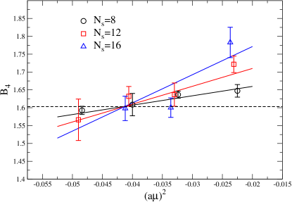
Figure 8: Binder cumulant for fixed quark mass ($am_{u,d}=0.005$) as a function of imaginary chemical potential and volume. The intersection signals the critical point.

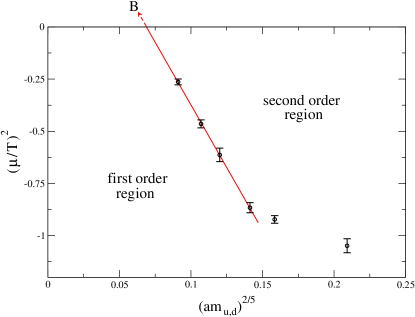
Figure 9: Data corresponding to the calculated critical points, the line is a fit according to tricritical scaling Eq. (4)

By using this expression we can, for each value of the bare quark mass $am_{u,d}$, find the corresponding critical value $(a\mu_{c})^{2}$. An example from our data is shown in Fig. 8, where (at fixed bare mass $am_{u,d}=0.005$) we scanned in imaginary chemical potential using up to four different volumes in order to identify the critical point and in all cases we reached lattice sizes such that $m_{\pi}L\gtrsim 3$ (in fact for all but the lightest mass used we arrived to $m_{\pi}L\gtrsim 4$). The fit is performed simultaneously on all the data at different volumes and $b_{4}^{(0)}$ is fixed to its infinite volume limit.

This procedure was carried out for six different values of the quark mass and the results are shown Fig. 9. The quark mass axis is rescaled with the appropriate critical exponent in order to display the scaling and extrapolation more clearly, as a straight line. Four data points accurately follow the tricritical scaling curve, which can then be used to estimate the position of the tricritical point “B” in the chiral limit, for which we find the large positive value

$$\left(\frac{\mu}{T}\right)^{2}_{\mathrm{tric}}=0.85(5)\ .$$ (8)

This definitely implies a first order behaviour for the two-flavor chiral phase transition on $N_{t}=4$ lattices. A crude estimate (obtained by using the interpolating formula for the masses of Ref. BGKT ) puts the critical pion mass corresponding to the second order point at $\mu=0$ to $m_{\pi}^{c}\sim$ 60 MeV.

V Conclusions

We have presented a new approach for the determination of the order of the chiral transition for $N_{f}=2$ QCD, based on the investigation of the phase diagram extended to imaginary chemical potential. In this approach, the chiral limit extrapolation is controlled and constrained by scaling considerations which follow from the universal behavior around a tricritical point. Present results show that, for QCD discretized on $N_{t}=4$ lattices with standard staggered fermions, the transition is first order in the chiral limit. This is consistent with some earlier lattice investigations DiG and with expectations from the fate of the $U(1)_{A}$ anomaly using overlap fermions overlap .

It should be stressed that the explored $N_{t}=4$ lattice is quite coarse, corresponding to $a\sim 0.3$ fm, and that results for $m_{c}(\mu)$ on finer lattices are needed before a continuum limit can be taken. For $\mu=0$ it is known that the three-flavor chiral first order region in Fig. 1 (left) shrinks significantly on finer lattices kim or with improved actions ding . Therefore, the issue about the presence of a first order chiral transition for $N_{f}=2$ QCD in the continuum remains non-trivial.

We have shown that the proposed approach is able to provide definite answers and constitutes a solid framework for future studies on the subject.

References

- (1) Y. Aoki, G. Endrodi, Z. Fodor, S. D. Katz and K. K. Szabo, Nature 443 (2006) 675 [hep-lat/0611014].
- (2) A. Bazavov, T. Bhattacharya, M. Cheng, C. DeTar, H. T. Ding, S. Gottlieb, R. Gupta and P. Hegde et al., Phys. Rev. D 85, 054503 (2012) [arXiv:1111.1710 [hep-lat]].
- (3) T. Bhattacharya, M. I. Buchoff, N. H. Christ, H. -T. Ding, R. Gupta, C. Jung, F. Karsch and Z. Lin et al., arXiv:1402.5175 [hep-lat].
- (4) P. de Forcrand and O. Philipsen, JHEP 0701 (2007) 077 [hep-lat/0607017].
- (5) P. de Forcrand and O. Philipsen, JHEP 0811 (2008) 012 [arXiv:0808.1096 [hep-lat]].
- (6) M. Fromm, J. Langelage, S. Lottini and O. Philipsen, JHEP 1201 (2012) 042 [arXiv:1111.4953 [hep-lat]].
- (7) H. Saito et al. [WHOT-QCD Collaboration], Phys. Rev. D 84 (2011) 054502 [Erratum-ibid. D 85 (2012) 079902] [arXiv:1106.0974 [hep-lat]].
- (8) H. Saito et al., arXiv:1309.2445 [hep-lat].
- (9) Y. Iwasaki, K. Kanaya, S. Kaya and T. Yoshie, Phys. Rev. Lett. 78 (1997) 179 [hep-lat/9609022].
- (10) A. A. Khan et al. (CP-PACS collaboration), Phys. Rev. D 63, 034502 (2000) [arXiv:hep-lat/0008011].
- (11) M. Fukugita, H. Mino, M. Okawa and A. Ukawa, Phys. Rev. Lett. 65, 816 (1990).
- (12) M. Fukugita, H. Mino, M. Okawa and A. Ukawa, Phys. Rev. D 42, 2936 (1990).
- (13) F. R. Brown, F. P. Butler, H. Chen, N. H. Christ, Z. Dong, W. Schaffer, L. I. Unger and A. Vaccarino, Phys. Rev. Lett. 65, 2491 (1990)
- (14) F. Karsch, Phys. Rev. D 49, 3791 (1994) [arXiv:hep-lat/9309022].
- (15) F. Karsch and E. Laermann, Phys. Rev. D 50, 6954 (1994) [arXiv:hep-lat/9406008].
- (16) S. Aoki et al. (JLQCD collaboration), Phys. Rev. D 57, 3910 (1998) [arXiv:hep-lat/9710048].
- (17) C. Bernard, C. DeTar, S. Gottlieb, U. M. Heller, J. Hetrick, K. Rummukainen, R. L. Sugar and D. Toussaint, Phys. Rev. D 61, 054503 (2000) [arXiv:hep-lat/9908008].
- (18) M. D’Elia, A. Di Giacomo and C. Pica, Phys. Rev. D 72, 114510 (2005) [hep-lat/0503030]; G. Cossu, M. D’Elia, A. Di Giacomo and C. Pica, arXiv:0706.4470 [hep-lat]; C. Bonati, G. Cossu, M. D’Elia, A. Di Giacomo and C. Pica, PoS LATTICE 2008, 204 (2008) [arXiv:0901.3231 [hep-lat]].
- (19) S. Ejiri et al., Phys. Rev. D 80, 094505 (2009) [arXiv:0909.5122 [hep-lat]].
- (20) R. D. Pisarski and F. Wilczek, Phys. Rev. D 29, 338 (1984).
- (21) E. Vicari, PoS LAT 2007, 023 (2007) [arXiv:0709.1014 [hep-lat]]. A. Butti, A. Pelissetto and E. Vicari, JHEP 0308, 029 (2003) [arXiv:hep-ph/0307036].
- (22) A. Pelissetto and E. Vicari, Phys. Rev. D 88, 105018 (2013) [arXiv:1309.5446 [hep-lat]].
- (23) S. Chandrasekharan and A. C. Mehta, Phys. Rev. Lett. 99, 142004 (2007) [arXiv:0705.0617 [hep-lat]].
- (24) M. Hasenbusch, J. Phys. A 34, 8221 (2001) [arXiv:cond-mat/0010463].
- (25) M. Hasenbusch, E. Vicari, Phys. Rev. B 84, 125136 (2011) [arXiv:1108.0491 [cond-mat.stat-mech]].
- (26) M. Campostrini, M. Hasenbusch, A. Pelissetto, P. Rossi, E. Vicari, Phys. Rev. B 63, 214503,(2001) [arXiv:cond-mat/0010360 [cond-mat.stat-mech]].
- (27) H. W. J. Blöte, E. Luijten, J. R. Heringa, J. Phys. A: Math. Gen. 28 6289 (1995) [arXiv:cond-mat/9509016].
- (28) F. Burger et al, Phys. Rev. D 87, 074508 (2013) [arXiv:1102.4530 [hep-lat]].
- (29) C. Bonati, P. de Forcrand, M. D’Elia, O. Philipsen and F. Sanfilippo, PoS LATTICE 2011, 189 (2011) [arXiv:1201.2769 [hep-lat]]. C. Bonati, P. de Forcrand, M. D’Elia, O. Philipsen and F. Sanfilippo, PoS LATTICE 2013, 219 (2013) [arXiv:1311.0473 [hep-lat]].
- (30) A. Roberge and N. Weiss, Nucl. Phys. B 275 (1986) 734.
- (31) P. de Forcrand and O. Philipsen, Nucl. Phys. B 642, 290 (2002) [arXiv:hep-lat/0205016].
- (32) M. D’Elia and M. P. Lombardo, Phys. Rev. D 67, 014505 (2003) [arXiv:hep-lat/0209146].
- (33) M. D’Elia, F. Di Renzo and M. P. Lombardo, Phys. Rev. D 76, 114509 (2007) [arXiv:0705.3814 [hep-lat]].
- (34) M. D’Elia and F. Sanfilippo, Phys. Rev. D 80, 111501 (2009) [arXiv:0909.0254 [hep-lat]]; C. Bonati, G. Cossu, M. D’Elia and F. Sanfilippo, Phys. Rev. D 83, 054505 (2011) [arXiv:1011.4515 [hep-lat]].
- (35) O. Philipsen and C. Pinke, Phys. Rev. D 89, 094504 (2014) [arXiv:1402.0838 [hep-lat]].
- (36) P. de Forcrand and O. Philipsen, Phys. Rev. Lett. 105, 152001 (2010) [arXiv:1004.3144 [hep-lat]].
- (37) K. Nagata and A. Nakamura, Phys. Rev. D 83, 114507 (2011) [arXiv:1104.2142 [hep-lat]].
- (38) A. Alexandru and A. Li, PoS LATTICE 2013, 208 (2013) [arXiv:1312.1201 [hep-lat]].
- (39) L.-K. Wu and X.-F. Meng, Phys. Rev. D 87, 094508 (2013) [arXiv:1303.0336 [hep-lat]]; arXiv:1405.2425 [hep-lat].
- (40) B. Lucini, A. Patella and C. Pica, Phys. Rev. D 75, 121701 (2007) [hep-th/0702167].
- (41) P. Cea, L. Cosmai, M. D’Elia, C. Manneschi and A. Papa, Phys. Rev. D 80, 034501 (2009) [arXiv:0905.1292 [hep-lat]]; P. Cea, L. Cosmai, M. D’Elia, A. Papa and F. Sanfilippo, Phys. Rev. D 85, 094512 (2012) [arXiv:1202.5700 [hep-lat]].
- (42) Y. Sakai, T. Sasaki, H. Kouno and M. Yahiro, Phys. Rev. D 82, 076003 (2010) [arXiv:1006.3648 [hep-ph]]; T. Sasaki, Y. Sakai, H. Kouno and M. Yahiro, Phys. Rev. D 84, 091901 (2011) [arXiv:1105.3959 [hep-ph]]; H. Kouno, M. Kishikawa, T. Sasaki, Y. Sakai and M. Yahiro, Phys. Rev. D 85, 016001 (2012) [arXiv:1110.5187 [hep-ph]].
- (43) G. Aarts, S. P. Kumar and J. Rafferty, JHEP 1007, 056 (2010) [arXiv:1005.2947 [hep-th]].
- (44) J. Rafferty, JHEP 1109, 087 (2011) [arXiv:1103.2315 [hep-th]].
- (45) J. Braun, L. M. Haas, F. Marhauser and J. M. Pawlowski, Phys. Rev. Lett. 106, 022002 (2011) [arXiv:0908.0008 [hep-ph]].
- (46) K. Morita, V. Skokov, B. Friman and K. Redlich, Phys. Rev. D 84, 076009 (2011) [arXiv:1107.2273 [hep-ph]].
- (47) K. Kashiwa, T. Hell and W. Weise, Phys. Rev. D 84, 056010 (2011) [arXiv:1106.5025 [hep-ph]].
- (48) V. Pagura, D. Gomez Dumm and N. N. Scoccola, Phys. Lett. B 707, 76 (2012) [arXiv:1105.1739 [hep-ph]].
- (49) D. Scheffler, M. Buballa and J. Wambach, Acta Phys. Polon. Supp. 5, 971 (2012) [arXiv:1111.3839 [hep-ph]].
- (50) K. Kashiwa and R. D. Pisarski, Phys. Rev. D 87, 096009 (2013) [arXiv:1301.5344 [hep-ph]].
- (51) K. Kashiwa, T. Sasaki, H. Kouno and M. Yahiro, Phys. Rev. D 87, 016015 (2013) [arXiv:1208.2283 [hep-ph]].
- (52) I. D. Lawrie, S. Sarbach Theory of Tricritical Points in C. Domb, J. L. Lebowitz (eds.) Phase transitions and critical phenomena, vol. 11. Academic Press (1987).
- (53) F. Wilczek, Int. J. Mod. Phys. A, 07, 3911 (1992).
- (54) K. Rajagopal, F. Wilczek, Nucl. Phys. B 399, 395 (1993) [hep-ph/9210253].
- (55) C. Bonati, G. Cossu, M. D’Elia and P. Incardona, Comput. Phys. Commun. 183, 853 (2012) [arXiv:1106.5673 [hep-lat]].
- (56) K. Binder, Phys. Rev. Lett. 47, 693 (1981).
- (57) K. Binder, Z. Phys. B - Condensed Matter 43, 119 (1981).
- (58) T. Blum, S. Gottlieb, L. Karkkainen, D. Toussaint, Phys. Rev. D 51, 5153 (1995) [arXiv:hep-lat/9410014].
- (59) G. Cossu et al., Phys. Rev. D 87 (2013) 114514 [arXiv:1304.6145 [hep-lat]].
- (60) P. de Forcrand, S. Kim and O. Philipsen, PoS LAT 2007 (2007) 178 [arXiv:0711.0262 [hep-lat]].
- (61) H. -T. Ding, J. Phys. Conf. Ser. 432 (2013) 012027 [arXiv:1302.5740 [hep-lat]].