Cooling and trapping of atoms and molecules by the counter-propagating pulses trains

Abstract

We discuss a possible one-dimensional trapping and cooling of atoms and molecules due to their non-resonant interaction with the counter-propagating light pulses trains. The counter-propagating pulses form a one-dimensional trap for atoms and molecules, and properly chosen the carrier frequency detuning from the transition frequency of the atoms or molecules keeps the “temperature” of the atomic or molecular ensemble close to the Doppler cooling limit. The calculation by the Monte-Carlo wave function method is carried out for the two-level and three-level schemes of the atom’s and the molecule’s interaction with the field, correspondingly. The discussed models are applicable to atoms and molecules with almost diagonal Frank-Condon factor arrays. Illustrative calculations where carried out for ensemble averaged characteristics for sodium atoms and SrF molecules in the trap. Perspective for the nanoparticle light pulses’s trap formed by counter-propagating light pulses trains is also discussed.

I Introduction

Optical cooling and trapping Chu (1998); Cohen-Tannoudji (1998); Phillips (1998) is the key stage of the experiments with cold atoms. Initially continuous laser radiation is used for this purpose, but pulsed laser applications for cooling Strohmeier et al. (1989); Mølmer (1991); Watanabe et al. (1996); Ilinova et al. (2011); Ilinova and Derevianko (2012a) and trapping Freegarde et al. (1995); Goepfert et al. (1997); Balykin (2005); Romanenko and Yatsenko (2011); Yanyshev et al. (2013) of atoms and molecules are also discussed now. Laser cooling of atoms by counter-propagated weak laser pulses was investigated in Mølmer (1991), but possible trapping was not recognized. The authors of Romanenko et al. (2013) analyzed the light pulses interaction with atoms for different detunings and found that simultaneous cooling and trapping of atoms are possible, provided that the carrier frequency detuning from the resonant atom-light interaction is properly chosen. More deep investigation of the cooling trap, based on the interaction of atoms with counter-propagating laser pulses, is described in Romanenko et al. (2014), where the numerical calculations for examples of the time evolution of a sodium atom in the trap where demonstrated.

The idea of the trap based on the atom’s interaction with the counter-propagating light pulses trains can be most easy explained for the case of two-level atoms in the field of $\pi$-pulses. Let light pulses propagate along the $z$-axis (see Fig. 1) and point $C$ is the point where the counter-propagating pulses “collide”. We assume that an atom at point $A$ was in the ground state before the recent interaction with pulse $R$ (this is true in most cases because of small time between the interaction of the atom with $R$ and $L$ pulses in comparison with the time between the interaction with $R$ and $R^{\prime}$ pulses Voĭtsekhovich et al. (1991)). As a result of the interaction with this pulse, the atom absorbed a photon and became excited.

Figure 1: Counter-propagating laser pulses form a trap for atoms near point $C$, where the pulses “collide”

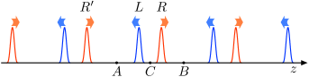
Its momentum was changed by the photon momentum $\hbar{}k$ in the positive $z$-axis direction. After being subjected to the action of pulse $L$, the atom emits a photon, becomes unexcited, and its momentum changes by another $\hbar k$ in the same direction. The interaction of the atom with the laser pulses repeats with period $T$, so the atom is subjected to the action of the average force $2\hbar k/T$ directed towards point $C$. A similar reasoning for an atom at point $B$ allow us to find that the atomic momentum changes by $-2\hbar k$, so that the average force acting on it is $-2\hbar k/T$, i.e. directed towards point $C$. From symmetry considerations we readily conclude that the light pressure force on the atom at point $C$ equals zero. Hence, counter-propagating light $\pi$-pulses can form a trap for an atom with the center at point $C$, where the counter-propagating pulses “collide”. As was pointed out in Freegarde et al. (1995); Goepfert et al. (1997), pulses with areas different from $\pi$ can also form a trap.

Recently a great progress in the manipulation of molecules by laser radiation was reported Barry et al. (2012). The authors of Barry et al. (2012) demonstrated deceleration of a beam of neutral strontium monofluoride molecules using radiative forces. The spectroscopic constants of this molecule satisfies the main conditions, which are required for the successful laser cooling. They are Di Rosa (2004): (1) a band system with strong one-photon transitions (i.e. large oscillator strength) to ensure the high photon-scattering rates needed for rapid laser cooling, (2) a highly-diagonal Franck-Condon array for the band system, and (3) no intervening electronic states to which the upper state could radiate and terminate the cycling transition. We note that it is the violation of the second criterion led to very high (about 97%) losses of the ground working state of Na₂ in the first observation of the light pressure force on molecules Voĭtsekhovich et al. (1994).

In this paper we calculate the characteristics of atomic and molecular ensembles in the trap formed by counter-propagating light pulses using Monte-Carlo method. We apply this method for different purpose: (1) simulation of an atom or a molecule states evolution by the Monte-Carlo wave function (MCWF) method Mølmer et al. (1993), and (2) calculation of ensemble averages of the coordinate, velocity and the second momenta of their values.

We illustrate the phenomenon of simultaneous cooling and trapping of atoms and molecules by counter-propagating light pulses trains using examples of sodium atoms and strontium monofluoride molecules, which have the level structure, suitable for light pressure force experiments Metcalf and van der Stratten (1999); Barry et al. (2012). We use the two-level model for an atom, as far as it adequately describes the cycling cooling transition Metcalf and van der Stratten (1999), and the three-level $\Lambda$-model for a molecule, as far as 0.9996 of the excited molecules radiatively decay to the two lower levels Barry et al. (2012). The atomic motion is described in the framework of classical mechanics, that corresponds to the narrow atomic wave packet in comparison with the wavelength. A perspective of trapping of nanoparticles is briefly discussed in the final part of the article.

This paper is organized as follows. In Sec. II we present the the models for atoms and molecules used in the paper. Section III describes the trains of the counter-propagating pulses which acts on the atoms and the molecules. Solving of Schrödinger equation by the Monte-Carlo wave function method is described in Sec. IV, closely following Mølmer et al. (1993). Section V contains the calculation of light pressure force and equations for mechanical motion of atoms and molecules. In Sec. VI we describe the numerical calculation routine used in the investigation. Results and discussion are presented in Sec. VII. Short conclusions are formulated in Sec. VIII.

II Models for atoms and molecules

We use the two-level model for description of the atom-field interaction. The transitions in atoms, which ensure the cycling interaction with the field within the two-level system, are listed, for example, in Metcalf and van der Stratten (1999).

Figure 2: Two-level scheme of the atom-field interaction (a) and three-level scheme of the molecule interaction with the field of laser radiation (b)

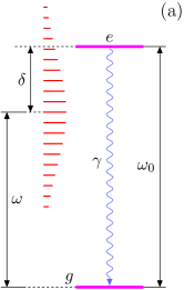
We denote the ground state with $g$ and the excited state with $e$ [see Fig. 2(a)]. The detuning of the carrier frequency $\omega$ from the transition frequency $\omega_{0}$ is $\delta=\omega_{0}-\omega$, and the rate of the atom’s spontaneous emission from the excited state is $\gamma$.

We describe the molecule’s interaction with the field by the three-level $\Lambda$-model, as depicted in Fig. 2(b). This model is composed of the excited state $e$ and the ground states $g_{1}$, $g_{2}$, separated by $\hbar\Delta$. The transition frequencies between the excited and each of the ground states are $\varpi_{1}$, $\varpi_{2}$, correspondingly. These frequencies differs for SrF molecule, which interaction with the laser pulses is simulated in this paper, by $\Delta/2\pi=14.9$ THz Barry et al. (2012). As far as $2\pi/\Delta$ is very small in comparison with the pulse duration $\tau$, we need two pairs of pulse trains, one of which is the counter-propagating pulses close to the resonance with $e\leftrightarrow{}g_{1}$ transition, and the other is the counter-propagating pulses close to the resonance with $e\leftrightarrow{}g_{2}$ transition. The carrier frequency of these pulses $\omega_{1}$, $\omega_{2}$ are detuned from the resonances by $\delta_{1}=\varpi_{1}-\omega_{1}$ and $\delta_{2}=\varpi_{2}-\omega_{2}$, correspondingly. We also introduce the spontaneous decay rates $\gamma_{1}$ and $\gamma_{2}$ from the upper state to the two lower states, which form the total decay rate $\gamma=\gamma_{1}+\gamma_{2}$.

III Laser pulses

We suppose that the pairs of pulses traveling in the same direction (and resonant to the different transitions) coincides in time. The spectrum of the laser field is a frequency comb with the difference between the teeth $2\pi/T$, where $T$ is the repetition period of the laser pulses.

The electric field of the trains of the counter-propagating pulses can be written as

$$\bm{\mathrm{E}}(t) = E_{1}\bm{\mathrm{e}}_{1}\sum\limits_{m}\cos[\omega_{1}{}t-k_{1}z+\varphi_{11,m}]f(\eta_{1,m})$$ (1)

$$+E_{1}\bm{\mathrm{e}}_{1}\sum\limits_{m}\cos[\omega{}_{1}t+k_{1}z+\varphi_{12,m}]f(\eta_{2,m})$$

$$+E_{2}\bm{\mathrm{e}}_{2}\sum\limits_{m}\cos[\omega_{2}{}t-k_{2}z+\varphi_{21,m}]f(\eta_{1,m})$$

$$+E_{2}\bm{\mathrm{e}}_{2}\sum\limits_{m}\cos[\omega_{2}{}t+k_{2}z+\varphi_{22,m}]f(\eta_{2,m}).$$

Here $k_{1}=\omega_{1}/c$, $k_{2}=\omega_{2}/c$ are the values of wave vectors for carrier frequencies $\omega_{1}$ and $\omega_{2}$, $\bm{\mathrm{e}}_{1}$ and $\bm{\mathrm{e}}_{2}$ are polarization vectors, $\varphi_{11,m}$, $\varphi_{12,m}$ and $\varphi_{21,m}$, $\varphi_{22,m}$ are the phases of the counter-propagating $m$-pulses for $t=0$ and $z=0$. Function $f(\eta)$ with maximum value $f(0)=1$ describe the shape of the pulse’s envelope,

$$\eta_{1,m} = \frac{1}{\tau}\left(t-mT-\frac{z}{c}\right),$$ (2)

$$\eta_{2,m} = \frac{1}{\tau}\left(t-mT+\frac{z}{c}\right),$$ (3)

where $z$ is the atom’s or molecule’s coordinate, $\tau$ is the pulse duration. The beginning of the coordinate axis and the order of the pulses numbering are chosen so that the counter-propagating pulses number $m$ meet each other at time instants $t=mT$ in point $z=0$, where $m$ is an arbitrary integer.

The pulse areas are defined by the integrals

$$\vartheta_{j}=\Omega_{j}\int_{-\infty}^{\infty}f(t/\tau)\,dt,\quad{}j=1,2,$$ (4)

where the Rabi frequencies are

$$\Omega_{j}=-\bm{\mathrm{d}}_{g_{j}e}\bm{\mathrm{e}}_{j}E_{j}/\hbar,\quad{}j=1,2.$$ (5)

The matrix elements $\bm{\mathrm{d}}_{g_{j}e}=\langle{g_{j}}|\bm{\mathrm{d}}|e\rangle$ of the dipole moments are assumed to be the real-valued quantities without loss of generality Shore (1990).

The case of the two-level model [Fig. 2(a)] is described by the equation of this subsection with $\gamma_{1}=\gamma$, $\gamma_{2}=0$, $\vartheta_{1}=\vartheta$, $\vartheta_{2}=0$, $\omega_{1}=\omega$, $\delta_{1}=\delta$, $\varpi_{1}=\omega_{0}$.

Usually the Gaussian-like pulses are used in simulations of the atom-field interactions Bergmann et al. (1998); Vitanov et al. (2001). These pulses are artificially cut off beyond certain limits in numerical calculation. We use $\cos^{4}$-like pulses which are close to Gaussian but restricted in time as real laser pulses,

$$f(\eta)=\left\{\begin{array}[c]{ll}\cos^{4}(\pi{}\eta),&|\eta{}|<1/2\\ 0,&|\eta{}|>1/2\end{array}\right..$$ (6)

The function $f(\eta)$ is close to the Gaussian distribution $f_{G}(\eta)=\exp\left(-2\pi^{2}\eta^{2}\right)$ in the interval where $f_{G}(\eta)$ is not very small. The area of the pulse with the envelope described by function (6) equals $\frac{3}{8}\Omega_{0}\tau$, that is approximately 0.94 times the area of the corresponding Gaussian pulse. The characteristic width of the latter is $\tau_{G}\approx 0.225\tau$. More close adjustment of $\cos^{n}$-like pulse to the Gaussian pulse is possible: the function $\cos^{n}(\pi t/\tau)$ tends to $\exp(-t^{2}/\tau_{G}^{2})$ with $\tau_{g}=\tau\sqrt{2}(\pi\sqrt{n})^{-1}$ for large even $n$ within the interval $\left|t\right|<\tau/2$ Romanenko (2006).

IV The wave function calculation

We describe the atomic state by the wave function which is constructed by the Monte-Carlo wave function (MCWF) method Mølmer et al. (1993). After averaging over the ensemble of atoms or molecules, this approach becomes equivalent to the solution of the density matrix equation. At the same time, in contrast to the latter, it allows one to give an illustrative interpretation for the separate atom’s or molecule’s motion.

The wave function obeys the Schrödinger equation

$$i\hbar\frac{\mathrm{d}}{\mathrm{d}t}|\psi\rangle=H|\psi\rangle,$$ (7)

where the Hamiltonian

$$H = \hbar\varpi_{1}|e\rangle\langle{}e|+\hbar\Delta|g_{2}\rangle\langle{}g_{2}|-\bm{\mathrm{d}}_{g_{1}e}|g_{1}\rangle\langle{}e|\bm{\mathrm{E}}(t)$$ (8)

$$-\bm{\mathrm{d}}_{eg_{1}}|e\rangle\langle{}g_{1}|\bm{\mathrm{E}}(t)-\bm{\mathrm{d}}_{g_{2}e}|g_{2}\rangle\langle{}e|\bm{\mathrm{E}}(t)$$

$$-\bm{\mathrm{d}}_{eg_{2}}|e\rangle\langle{}g_{2}|\bm{\mathrm{E}}(t)-\frac{i\hbar}{2}\left(\gamma_{1}+\gamma_{2}\right)|e\rangle\langle{}e|,$$

which is used for the construction of the wave function by MCWF method, differs in the relaxation term from the Hamiltonian which is used in the density matrix equation.

Hamiltonian (8) is non-Hermitian, hence the absolute value of the wave function determined from the Schrödinger equation (7) changes with time. In the MCWF method, normalization of the wave function should be carried out after every small time step. Besides that, the condition of a quantum jump within each time interval has to be checked Mølmer et al. (1993).

We use the first order method for calculation of Monte-Carlo wave function Mølmer et al. (1993). More precise the second and the fourth order methods are described in Steinbach et al. (1995).

Let the wave function $|\psi(t)\rangle$ is normalized to unity at the time moment $t$. After a small time step $\Delta t$ the wave function $|\psi(t)\rangle$ is transformed into

$$|\psi^{(1)}(t+\Delta{}t)\rangle=\left(1-\frac{i\Delta{}t}{\hbar}{{H}}\right)|\psi(t)\rangle$$ (9)

according to Schrödinger equation (7). The squared norm of the wave function equals

$$\langle\psi^{(1)}(t+\Delta{}t)|\psi^{(1)}(t+\Delta{}t)\rangle=1-\Delta{}P,$$ (10)

where

$$\Delta{}P = \frac{i\Delta{}t}{\hbar}\langle\psi(t)|H-H^{+}|\psi(t)\rangle$$ (11)

$$= \left(\gamma_{1}+\gamma_{2}\right)\langle\psi(t)|e\rangle\langle{}e|\psi(t)\rangle\Delta{}t.$$

Now we take into account a possibility of quantum jump. If the value of the random variable $\epsilon$, which is uniformly distributed between zero and unity, is larger than $\Delta{}P$ (it is true in the most cases, as far as $\Delta{}P\ll 1$), there is no jump. Then the wave function at the time moment $t+\Delta t$ equals

$$|\psi(t+\Delta{}t)\rangle=|\psi^{(1)}(t+\Delta{}t)\rangle/\sqrt{1-\Delta{}P},\quad\Delta{}P<\epsilon.$$ (12)

In the opposite case, $\epsilon<\Delta P$, the jump occurs, and the wave functions becomes

$$|\psi(t+\Delta{}t)\rangle=|g_{1}\rangle$$ (13)

with probability $p_{1}=\gamma_{1}/(\gamma_{1}+\gamma_{2})$, or

$$|\psi(t+\Delta{}t)\rangle=|g_{2}\rangle$$ (14)

with probability $p_{2}=\gamma_{2}/(\gamma_{1}+\gamma_{2})$. If the value of the random variable $\epsilon$, uniformly distributed between 0 and 1, is less then $p_{1}$, the wave function is (13), otherwise it is (14).

It is convenient to separate the rapid component, varying with the frequency $\varpi_{1}$, in the wave function. For this purpose we seek for the solution of (7) in the form

$$|\psi\rangle=C_{g_{1}}|g_{1}\rangle+C_{{2}}e^{-i\Delta{}t}|g_{2}\rangle+C_{e}e^{-i\varpi_{1}t}|e\rangle.$$ (15)

After applying rotating wave approximation Shore (1990) to the Schrödinger equation we find, assuming $\Delta\ll\varpi_{1}$, the equations for probability amplitudes

$$\frac{d}{dt}C_{g_{1}} = -\frac{i}{2}\Omega_{1}e^{-ikz-i\delta_{1}t}\sum\limits_{m}e^{i\varphi_{11,m}}f(\eta_{1,m})C_{e}{}$$ (16)

$$-\frac{i}{2}\Omega_{1}e^{ikz-i\delta_{1}t}\sum\limits_{m}e^{i\varphi_{12,m}}f(\eta_{2,m})C_{e}$$

$$\frac{d}{dt}C_{g_{2}} = -\frac{i}{2}\Omega_{2}e^{-ikz-i\delta_{2}t}\sum\limits_{m}e^{i\varphi_{21,m}}f(\eta_{1,m})C_{e}$$ (17)

$$-\frac{i}{2}\Omega_{2}e^{ikz-i\delta_{2}t}\sum\limits_{m}e^{i\varphi_{22,m}}f(\eta_{2,m})C_{e},$$

$$\frac{d}{dt}C_{{e}} = -\frac{i}{2}\Omega_{1}e^{ikz+i\delta_{1}t}\sum\limits_{m}e^{-i\varphi_{11,m}}f(\eta_{1,m})C_{g_{1}}$$ (18)

$$-\frac{i}{2}\Omega_{1}e^{-ikz+i\delta_{1}t}\sum\limits_{m}e^{-i\varphi_{12,m}}f(\eta_{2,m})C_{g_{1}}$$

$$-\frac{i}{2}\Omega_{2}e^{ikz+i\delta_{2}t}\sum\limits_{m}e^{-i\varphi_{21,m}}f(\eta_{1,m})C_{g_{2}}$$

$$-\frac{i}{2}\Omega_{2}e^{-ikz+i\delta_{2}t}\sum\limits_{m}e^{-i\varphi_{22,m}}f(\eta_{2,m})C_{g_{2}}$$

$$-\frac{\gamma_{1}+\gamma_{2}}{2}C_{e},$$

which are to be solved numerically simultaneously with the quantum jump testing.

Most time (during the time interval between the light pulses) the field does not influence the atom or the molecule. In this case the analytical solution of the Eqs.  (16)–(18) is possible. Let the initial atom’s or molecule’s state is

$$|\psi(0)\rangle=C_{g_{1}}(0)|g_{1}\rangle+C_{g_{2}}(0)|g_{2}\rangle+C_{e}(0)|e\rangle.$$ (19)

If no quantum jump occurs within the time interval $[0,t]$, we find from the Eqs. (16)–(18) the normalized wave function

$$|\psi(t)\rangle = C_{g_{1}}(t)|g_{1}\rangle+C_{g_{2}}(t)e^{-i\Delta{}t}|g_{2}\rangle$$ (20)

$$+C_{e}(t)e^{-i\varpi_{1}t}|e\rangle,$$

where

$$C_{g_{1}}(t) = {C_{g_{1}}(0)}/{D},$$ (21)

$$C_{g_{2}}(t) = {C_{g_{2}}(0)}/{{D}},$$ (22)

$$C_{e}(t) = {C_{e}(0)e^{{-\frac{1}{2}\left(\gamma_{1}+\gamma_{2}\right)t}}}/{D}$$ (23)

and

$$D=\sqrt{|C_{g_{1}}(0)|^{2}+|C_{g_{2}}(0)|^{2}+|C_{e}(0)|^{2}e^{-(\gamma_{1}+\gamma_{2})t}}.$$ (24)

The probability of the absence of a quantum jump within the time interval $[0,t]$ is Mølmer et al. (1993)

$$P(t)=|C_{1}(0)|^{2}+|C_{2}(0)|^{2}+|C_{e}(0)|^{2}e^{-(\gamma_{1}+\gamma_{2})t}.$$ (25)

The expression (25) is consistent with the probability $|C_{1}(0)|^{2}+|C_{2}(0)|^{2}$ of no quantum jump for $t\to\infty$ and the exponential decay of the excited state in the ensemble of atoms or molecules.

So, in sum, in the absence of laser radiation within the time interval $[0,t]$ the atom or molecule is described by the state (20) at the time instant $t$ with the probability (25). The other possible states are

$$|\psi(t)\rangle=|g_{1}\rangle$$ (26)

with the probability $\gamma_{1}\left[1-P(t)\right]/\left(\gamma_{1}+\gamma_{2}\right)$ and

$$|\psi(t)\rangle=|g_{2}\rangle.$$ (27)

with the probability $\gamma_{2}\left[1-P(t)\right]/\left(\gamma_{1}+\gamma_{2}\right)$.

V Atom’s and molecule’s motion

Cooling of atoms in one-dimensional molasses was successfully simulated by MCWF method in Mølmer et al. (1993). In this case only the atomic momentum distribution function matters. Analyzing possible simultaneous cooling and trapping of atoms or molecules in the considering trap, we need both the spatial and momentum distribution functions. Quantum-mechanical calculation of the atomic motion in the trap should start from the wave package with spatial width much less then the laser radiation wavelength. As consequence, a lot of momentum states of the atom both in the ground an excited state are involved in the calculation.

The computation time can be substantially reduced for the case of weak laser fields, when the momentum diffusion of the atoms could be treated as caused by counter-propagating laser pulses independently. In this case we consider the atom’s motion in the framework of classical mechanics and need to know the light pressure force, which the atoms undergo. This force can be calculated from the density matrix and the electric field of the pulses Minogin and Letokhov (1987); Metcalf and van der Stratten (1999),

$$F=\sum\limits_{j=1}^{2}(\varrho_{g_{j}e}\bm{\mathrm{d}}_{eg_{j}}+\varrho_{eg_{j}}\bm{\mathrm{d}}_{g_{j}e})\frac{\partial\bm{\mathrm{E}}}{\partial z},$$ (28)

where the density matrix elements are expressed in terms of $C_{g_{1}}$, $C_{g_{2}}$ and $C_{e}$ as follows:

$$\varrho_{g_{j}g_{j}} = |C_{j}|^{2},\quad{}j=1,2,$$ (29)

$$\varrho_{ee} = |C_{e}|^{2},$$ (30)

$$\varrho_{eg_{1}} = C_{1}^{*}C_{e}e^{-i\varpi_{1}{}t},$$ (31)

$$\varrho_{g_{1}\!e} = C_{1}C_{e}^{*}e^{i\varpi_{1}{}t},$$ (32)

$$\varrho_{eg_{2}} = C_{2}^{*}C_{e}e^{-i\varpi_{2}{}t},$$ (33)

$$\varrho_{g_{2}e} = C_{2}C_{e}^{*}e^{i\varpi_{2}{}t}.$$ (34)

We assume that the pulse duration considerably exceeds the inverse carrier frequency, $\omega_{1}\tau\gg 1$, $\omega_{2}\tau\gg 1$, therefore we neglect the derivative of the pulse’s envelope in calculation of the time derivative of the field strength, as far as $|\frac{\partial f(\eta_{j,m})}{\partial z}|\ll{}k_{j}f(\eta_{j,m})$ ($j=1,2$).

After averaging over the period of oscillations with the frequency $\omega_{1}$, the expression (28) in the field (1) gives

$${{{F}}} = \left[\hbar{}k_{1}\Omega_{1}\mathop{\mathrm{Im}}C_{1}C_{e}^{*}e^{i\delta_{1}t+ik_{1}z}\sum\limits_{m}e^{-i\varphi_{11,m}}f(\eta_{1,m})\right.$$ (35)

$$+\hbar{}k_{2}\Omega_{2}\mathop{\mathrm{Im}}C_{2}C_{e}^{*}e^{i\delta_{2}t+ik_{2}z}\sum\limits_{m}e^{-i\varphi_{21,m}}f(\eta_{1,m})$$

$$-\hbar{}k_{1}\Omega_{1}\mathop{\mathrm{Im}}C_{1}C_{e}^{*}e^{i\delta_{1}t-ik_{1}z}\sum\limits_{m}e^{-i\varphi_{12,m}}f(\eta_{2,m})$$

$$\left.-\hbar{}k_{2}\Omega_{2}\mathop{\mathrm{Im}}C_{2}C_{e}^{*}e^{i\delta_{2}t-ik_{2}z}\sum\limits_{m}e^{-i\varphi_{22,m}}f(\eta_{2,m})\right]$$

$$\times\left[|C_{1}|^{2}+|C_{2}|^{2}+|C_{e}|^{2}\right]^{-1}.$$

The dependences of the atom’s coordinate $z$ on time we find from the Newton’s equation

$$\ddot{z}=F/M,$$ (36)

where $M$ is the atom’s mass. We consider the case $\left|\varpi_{1}-\varpi_{2}\right|\ll\varpi_{1}$, and assume $k_{1}=k_{2}$ in (35).

The Eq. (36) does not take into account the momentum change due to spontaneous emission of photons. Every event of spontaneous emission of a photon change the atom’s or the molecule’s velocity by $\hbar{}\bm{k}/M$ in the random direction with the probability $1-P(t)$, where $P$ is determined by (25). Besides that, the velocity also changes due to fluctuations of absorption and stimulated emission of photons.

VI Numerical calculation routine

To simulate the atom’s or molecule’s motion, we simultaneously solve the Eqs. (16)–(18) and (36), where the light pressure force we find from (35). Besides that, we take into account both the atomic momentum’s change due to the spontaneous emission of photons and fluctuation of stimulated (absorption and emission) processes. In our model calculations we postulate that spontaneous emission occurs with equal probability in two directions along the light beam, so the atom’s or molecule’s momentum changes by $\pm\hbar k$. This assumption in analyses of Doppler cooling leads to minimum temperature Adams and Riis (1997)

$$T_{\min}=\hbar\gamma/2k_{B},$$ (37)

where $k_{B}$ is the Boltzmann constant, $\gamma$ is the rate of the spontaneous emission of radiation by the excited atom.

The light pressure force (28) gives correct value for the ensemble averaged force, but the momentum diffusion phenomenon is not correctly taken into account. To analyze the motion of atoms or molecules in the trap we need to add stochastic change of the momentum, zero in average, that gives correct momentum diffusion coefficient. We analyze the low intensity case, when the population of the excited state is small and the light pressure force and the momentum diffusion approximately equal to the sum of the corresponding values for each of the counter-propagating traveling waves. Here we describe the momentum diffusion of atoms in the field of one traveling wave following Minogin and Letokhov (1987).

Let the momentum of an atom at the time instant $t$ is $\mathbf{p}_{0}$. Then at the time instant $t+\Delta t$ the momentum is

$$\mathbf{p}=\mathbf{p}_{0}+\hbar{}\mathbf{k}(N_{+}-N_{-})-\sum_{s}\hbar{}\mathbf{k}_{s}.$$ (38)

Here the second term gives the change of momentum due absorption and stimulated emission, when the photons with the wave vectors $\mathbf{k}$ (directed along $z$-axis) are absorbed and emitted. The quantities $N_{+}$ and $N_{-}$ are the numbers of the absorbed and emitted photons. The third term in (38) is responsible for the momentum change due to the spontaneous emission of the photons with the wave vectors $\mathbf{k}_{s}$.

The ensemble average of the momentum (38) is

$$\langle\mathbf{p}\rangle=\langle\mathbf{p}_{0}\rangle+\hbar{}\mathbf{k}(\langle N_{+}\rangle-\langle N_{-}\rangle),$$ (39)

where $\langle\mathbf{p}_{0}\rangle$ is the initial average momentum, $\langle N_{+}\rangle$ is the average number of the absorbed photons, $\langle N_{-}\rangle$ is the average number of the photon emitted by atoms in the process of stimulated emission. The photons emitted in the process of spontaneous emission does not change the average momentum,

$$\Bigl{\langle}\sum_{s}\mathbf{k}_{s}\Bigr{\rangle}=0.$$ (40)

The difference of (38) and (39) gives the momentum fluctuation,

$$\Delta\mathbf{p}=\mathbf{p}-\langle\mathbf{p}\rangle=(\mathbf{p}-\langle\mathbf{p}_{0}\rangle)+\hbar\mathbf{k}\Delta N_{i}-\sum_{s}\hbar\mathbf{k}_{s},$$ (41)

where $\Delta N_{i}=N_{i}-\langle N_{i}\rangle$ is the variation of the difference $N_{i}=N_{+}-N_{-}$ from the corresponding ensemble average value.

The average square of the momentum fluctuations along $z$-axis is

$$\langle\Delta{p}_{z}^{2}\rangle=\langle\Delta{p}_{0z}^{2}\rangle+\hbar^{2}{k}^{2}\langle(\Delta N_{i})^{2}\rangle+\hbar^{2}{k}^{2}\langle\cos^{2}\theta\rangle\langle N_{s}\rangle.$$ (42)

Here $\theta$ is the angle between the direction of the photon’s spontaneous emission and $z$-axis, $\langle N_{s}\rangle$ is the average number of the spontaneously emitted photons. The first term in the r.h.s. of (42) gives the initial momentum spreading, the second term is due to stimulated processes (absorption and emission), the third term is due to spontaneous emission.

Let’s find $\langle(\Delta N_{i})^{2}\rangle$ assuming the Poisson photons statistics. In this case

$$\langle(\Delta N_{i})^{2}\rangle=\langle N_{i}\rangle.$$ (43)

Noting that $\langle N_{i}\rangle=\langle N_{s}\rangle$, we finally find

$$\langle\Delta{p}_{z}^{2}\rangle=\langle\Delta{p}_{0z}^{2}\rangle+\hbar^{2}{k}^{2}\langle N_{s}\rangle+\hbar^{2}{k}^{2}\langle\cos^{2}\theta\rangle\langle N_{s}\rangle.$$ (44)

This equation shows the way for numerical modeling of momentum diffusion process in the field of traveling wave. Each random momentum change due to spontaneous emission is accompanied by stimulated process, in which the momentum of the atom is changed by $\pm\hbar k$.

Now consider the case of counter-propagating laser pulses. When counter-propagating laser pulses are weak, spontaneous emission follows each absorbed photon, so the fluctuation events of the atomic or molecular velocity change due to light induced processes occur as frequently as events of spontaneous emission. This point is the background of our computer simulation of atoms and molecules movement in the field of laser radiation.

In our calculation we assume the model of $\pm\hbar k$ change of the momentum due to spontaneous emission ($\theta$ equals $0$ or $\pi$ with equal probability). We use different approaches to solving these Eqs. (16)–(18) and (36), (35) during the atom’s interaction with the pulses and free evolution of the atom. In the first case the solution to the set of equations is found by using Runge-Kutta fourth order method with fixed step size. After every step we check if a quantum jump occurs and normalize the wave function. If a jump occurs, the atom’s velocity changes by $\Delta{}v=\hbar{}k(\epsilon_{1}-0.5)|/(M|\epsilon_{1}-0.5|)+\hbar{}k(\epsilon_{2}-0.5)|/(M|\epsilon_{2}-0.5|)$, where $\epsilon_{1,2}$ are random numbers with a uniform distribution in the interval $[0,1]$. In the second case, when the field does not act on the atom, we do not need to divide the considered time interval by small subintervals and check if the quantum jump occurs in every subinterval. Knowing the probability (25) of the absence of a quantum jump within the time interval $[0,t]$, we simulate the time moment of the quantum jump. The scheme of calculation is following. We compare the value of the uniformly distributed in the interval $[0,1]$ random variable $\epsilon$ with $|C_{1}(0)|^{2}+|C_{2}(0)|^{2}$ at the beginning of the time interval. A jump occurs if $\epsilon>|C_{1}(0)|^{2}+|C_{2}(0)|^{2}$, and does not otherwise. In the latter case the wave function is described by Eqs. (15), (21)–(23). If a jump occurs, we simulate the time moment of the quantum jump. We take a random $\epsilon$, which is uniformly distributed in the interval $[0,1]$. For the exponential distribution of probability, $P_{e}=e^{-(\gamma_{1}+\gamma_{2})t}$, the quantity $t_{jump}=-\left(\ln\epsilon\right)(\gamma_{1}+\gamma_{2})^{-1}$ simulates the time moment when the jump occurs Sobol (1974). If $t_{jump}$ exceeds the time interval between the laser pulses, we calculate the probability amplitudes (21)–(23) at the beginning of the next pulse, otherwise we calculate the atom’s velocity change $\Delta{}v=\hbar{}k(\epsilon_{1}-0.5)|/(M|\epsilon_{1}-0.5|)+\hbar{}k(\epsilon_{2}-0.5)|/(M|\epsilon_{2}-0.5|)$ at $t_{jump}$ using random numbers $\epsilon_{1,2}$ with a uniform distribution in the interval $[0,1]$. The atom’s or molecule’s state is (26), with the probability $\gamma_{1}\left[1-P(t)\right]/\left(\gamma_{1}+\gamma_{2}\right)$, or (27), with the probability $\gamma_{2}\left[1-P(t)\right]/\left(\gamma_{1}+\gamma_{2}\right)$. To choose between these states, we compare $\gamma_{1}/(\gamma_{1}+\gamma_{2})$ with a new random value $\epsilon$. When $\epsilon<\gamma_{1}/(\gamma_{1}+\gamma_{2})$, the state of the atom or the molecule is described by (26), otherwise by wave function (27).

The described approach substantially reduces the calculation time in comparison with Runge-Kutta method during whole time of the atom’s or the molecule’s motion.

To estimate the temperature of the captured atoms or molecules, we average the velocity and the squared velocity over the ensemble of particles.

VII Results and discussion

In this section we describe the results of the numerical simulation of atoms and molecules motion in the trap formed by the trains of counter-propagating light pulses. In contrast to the results of Romanenko et al. (2013, 2014), where the evolution of two-level atoms was investigated, here we also study statistical characteristics of the atomic and molecular ensembles.

We analyze the simplest models of the atom-field and the molecule-field interaction. It is well known that the cycling atom-field interaction can be realized between two states of some atoms Metcalf and van der Stratten (1999). As an example of such interaction, we chose transition $3^{2}S_{1/2}{-}3^{2}P_{3/2}$ in the sodium atom. The simplest molecule-field interaction model include three levels. The transitions coupling the state $A^{2}\Pi_{1/2}(v^{\prime}=0,J^{\prime}=1/2)$ with the states $X^{2}\Sigma_{1/2}^{+}(v=0,N=1)$ and $X^{2}\Sigma_{1/2}^{+}(v=1,N=1)$ of $\mathrm{SrF}$ form the almost close three-level $\Lambda$-scheme Barry et al. (2012). The spontaneous emission from the upper state leads the molecule to the lower states with the probability 0.9996. Including the state $X^{2}\Sigma_{1/2}^{+}(v=2,N=1)$ into the considered model gives the probability of the spontaneous transition to the three lower states more then $0.9999$, but we do not add this state, possibly sacrificing the simulation accuracy for the sake of greater physical clarity. Anyway, an additional light fields can return the molecules which is lost from the scheme due to the spontaneous emission, as it was realized in experiment Barry et al. (2012).

VII.1 Two-level model

Nowadays the investigation of simultaneous trapping and cooling of atoms by the counter-propagating laser pulses are presented in two papers, Romanenko et al. (2013, 2014), for the two-level model of the atom-field interaction. The authors of the first paper studied the momentum diffusion of the two-level atoms in an optical trap formed by sequences of the counter-propagating light pulses trains and discovered that proper detuning of carrier frequency of laser pulses from the resonance with the atom’s transition frequency leads to cooling of the atomic ensemble. The other sign of the detuning, as well as the resonant interaction of the field with atoms, leads to “heating” of the atomic ensemble. The conclusions of Romanenko et al. (2013) are based on the computer simulation of the motion of an atom in the trap for hypothetical atomic and atom-field interaction parameters. In Romanenko et al. (2014) the motion of $\mathrm{{}^{23}Na}$ atom in the trap was analyzed. Here we take the next step in the pulse trap investigation, which includes the simulation of the atomic ensemble characteristics.

Possible cooling of atoms in the trap can be easily explained for weak pulses, $\vartheta\ll\gamma T$, where $\vartheta\equiv\vartheta_{1}$ is the pulse area, $\gamma\equiv\gamma_{1}$. In this case the atom mostly interacts with the spectral component of the pulses trains which is closest to the transition frequency. Let the carrier frequency of the pulses is tuned below the transition frequency in the atom. Then the atoms, due to Doppler effect, always absorb more photons from the laser beam opposite to their direction of motion. As a result, “a friction force” arises and cools the atoms down to the Doppler cooling limit (37). This limit is caused by the competition between the cooling due to the friction force and heating due to the momentum diffusion. For large pulse areas the detuning of the carrier frequency from the resonance with the transition frequency in the atom, needed for atoms cooling, change sign Romanenko et al. (2014).

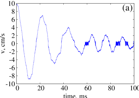
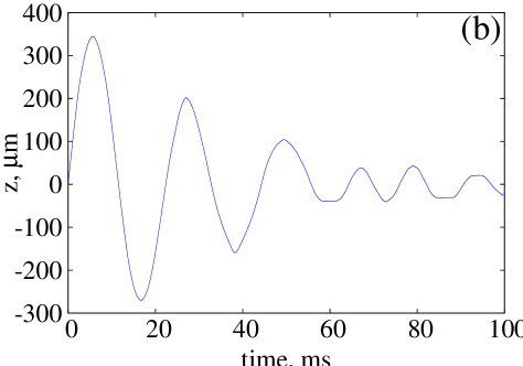
We consider an optical trap which extends from $z=-100$ mm to $z=100$ mm relative to the point, where counter-propagating light pulses “collide”, and trace the motion of an atom until it moves inside the trap. Level $g_{2}$ is not taken into account in the simulation of ${}^{23}\mathrm{Na}$ motion in the trap. Besides that, we suppose $\varphi_{11,m}=\varphi_{12,m}=0$ in (16), (18). Figure 3 shows an example of the atom’s motion in the field of the counter-propagating sequences of 1-ps light pulses with repetition frequency 100 MHz.

Figure 3: An example of the sodium atom’s motion in the field of the counter-propagating sequences of light pulses: (a) $v(t)$ and (b) $z(t)$. Parameters: $\tau=1$ ps, $T=10$ ns, $\vartheta=0.05\pi$, $\gamma=2\pi\times 10$ MHz, $\delta=2\pi\times 5$ MHz, $\lambda=589$ nm, $M=23$ Da. The atom starts at the center of the trap with initial velocity $v_{0}=5$ m/s.

Very quickly (0.14 ms after the beginning of the interaction with the field) the atom slows down to zero velocity and then its velocity fluctuates in the region $\pm 1$ m/s. The atom returns to the center of the trap approximately after 4.7 ms and then fluctuates in the region $\pm 0.25$ mm. The velocity capture range of the trap for the parameters specified in Fig. 3 extends at least from $v=-20$ m/s to $v=+20$ m/s (temperature of atoms about 1 K).

To estimate the measure of cooling in the trap, we introduce the “temperature” of the atomic ensemble by the expression

$$T_{a}=\frac{m\langle{}v^{2}\rangle}{k_{B}},$$ (45)

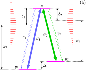
where $k_{B}$ is the Boltzmann constant. The value of $T_{a}$ coincides with the real temperature of the ensemble in the case of Maxwell velocity distribution. We expect that cooling process in the trap is close to the Doppler cooling Adams and Riis (1997); Metcalf and van der Stratten (1999), anyway for the case of weak field. This expectation is confirmed by comparison of smooth curve and dots in the Fig.4, where the dots were calculated from Eq. (45) with averaging over 1000 sodium atoms

Figure 4: The dependence of the temperature of 1000 sodium atom’s in the trap formed by the counter-propagating sequences of light pulses on the pulse’s carrier frequency detuning on the atomic transition frequency. Parameters: $\tau=1$ ps, $T=10$ ns, $\vartheta=0.05\pi$, $\gamma=2\pi\times 10$ MHz, $\lambda=589$ nm, $M=23$ Da.

and smooth curve represents the dependence of the atoms temperature on the detuning of the frequency of the weak monochromatic standing wave from the atomic transition frequency Adams and Riis (1997)

$$T_{sw}=\frac{1}{2}T_{\min}\left(\frac{2\delta}{\gamma}+\frac{\gamma}{2\delta}\right).$$ (46)

For sodium atoms $T_{\min}=240\,\mu$K Metcalf and van der Stratten (1999). The temperature is minimal, as in the case of the standing wave, for $\delta=\gamma/2$. The difference between the curve and the dots, according to our calculations, becomes less for smaller pulse’s areas.

The spatial capture range of the trap depends on $\delta$ and $\vartheta$. The first dependence is depicted in Fig. 5.

Figure 5: The dependence of the spatial capture range of the trap $\Delta z=\sqrt{\left\langle z^{2}\right\rangle-\left\langle z\right\rangle^{2}}$ on the frequency detuning $\delta$. The parameters are the same as in Fig. 4.

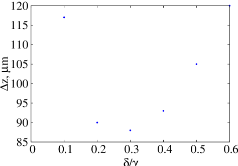
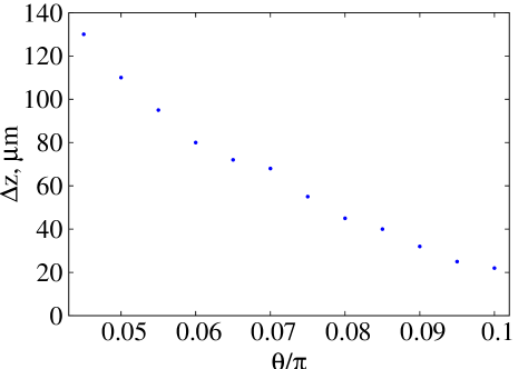
The minimal capture range does not coincide with the minimal temperature; it reaches approximately for $\delta=0.3\gamma$. For the parameters used in modeling this dependence, the atoms are localized in the region of the pulses’ overlapping. This region became narrower when pulse area increases (see Fig. 6).

Figure 6: The dependence of the spatial capture range of the trap $\Delta z=\sqrt{\left\langle z^{2}\right\rangle-\left\langle z\right\rangle^{2}}$ on the pulse area for $\delta=0.5\gamma$. The other parameters are the same as in Fig. 4.

VII.2 Three-level model

We simulate the dynamics of the three level system for the parameters, that are close to the interaction of $\mathrm{SrF}$ with CW laser radiation Barry et al. (2012). Our consideration neglects the probability 0.0004 of the molecule to leave the $\Lambda$-scheme in the process of spontaneous emission from the excited level (see Fig. 2). The spontaneous emission rate from the excited state is $\gamma=\gamma_{1}+\gamma_{2}=2\pi\times 7$ MHz, branching ratio $\gamma_{2}/\gamma_{1}=0.02$. Considering the equal energy of the pulses, we came to conclusion that $\vartheta_{2}/\vartheta_{1}=d_{eg_{2}}/d_{eg_{1}}=\sqrt{\gamma_{2}/\gamma_{1}}=0.14$. The wavelengths of the transitions are $\lambda_{1}=663.3$ nm ($e\Leftrightarrow g_{1}$), $\lambda_{2}=686.0$ nm ($e\Leftrightarrow g_{2}$). In calculation of the photon momentum for each transition we neglect the difference between $\lambda_{1}$ and $\lambda_{2}$. Repetition period of the pulses is chosen $T=23.8$ ns. It corresponds to the period of frequency modulation of laser radiation in the experiment Barry et al. (2012), that provides the excitation of all superfine sublevels of the ground states. Detunings $\delta_{1}$ and $\delta_{2}$ should not correspond to the two-photon resonance condition $\delta_{2}-\delta_{1}=2\pi n/T$, where $n$ is integer, to avoid the coherent population trapping, otherwise the population of the excited state becomes zero and the light pressure force vanishes Ilinova and Derevianko (2012a, b). As in the case of the two-level model, the pulse duration is $\tau=1$ ps.

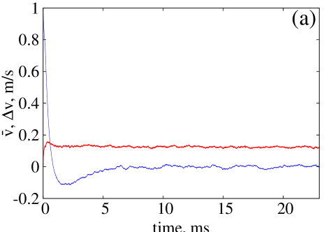
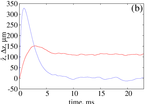
Figure 7 shows an example of the atom’s motion in the field of the counter-propagating sequences of 1-ps light pulses.

Figure 7: An example of SrF molecule motion in the field of the counter-propagating sequences of light pulses: (a) $v(t)$ and (b) $z(t)$. Parameters: $\tau=1$ ps, $T=23.8$ ns, $\vartheta_{1}=0.1\pi$, $\vartheta_{2}=0.014\pi$, $\gamma=2\pi\times 7$ MHz, $\delta_{1}=2\pi\times 3.5$ MHz, $\delta_{2}=2\pi\times 7$ MHz, $\lambda=663.3$ nm, $M=107$ Da. The molecule starts at the center of the trap with initial velocity $v_{0}=1$ m/s.

Very quickly (0.34 ms after the beginning of the interaction with the field) the atom slows down to zero velocity and then its velocity fluctuates in the region $\pm 0.4$ m/s. The atom returns to the center of the trap approximately after 5.6 ms and then fluctuates in the region $\pm 0.25$ mm.

Sometimes, in 2% cases, the excited molecule relax to $g_{2}$ state. As a result, we see in Fig. 7 several almost horizontal pieces. These pieces corresponds to staying the molecule in the state $g_{2}$, where the interaction of the molecule with the field is much weaker than in the state $g_{1}$. Between these pieces the velocity time dependence resembles one of the two-level atom in the field of the counter-propagating pulse trains, shown in Fig. 3(a). The capture range of the trap for the parameters specified in Fig. 7 extends at least from $v=-12$ m/s to $v=+12$ m/s.

The time dependences of average coordinate $\bar{z}=\left\langle z\right\rangle$, average velocity $\bar{v}=\left\langle v\right\rangle$ and $\Delta v=\sqrt{\left\langle v^{2}\right\rangle-\left\langle v\right\rangle^{2}}$, $\Delta z$ for an ensemble of 400 molecules are depicted in Fig. 8.

Figure 8: The time dependences of average coordinate $\bar{z}=\left\langle z\right\rangle$ and velocity $\bar{v}=\left\langle v\right\rangle$, $\Delta v=\sqrt{\left\langle v^{2}\right\rangle-\left\langle v\right\rangle^{2}}$ and $\Delta z$ for an ensemble of 400 molecules. The parameters are the same of Fig. 7.

Approximately after 10 $\mu$s the ensemble of molecules with equal initial velocity become localized in the vicinity of the coordinate origin with $\Delta z=112\,\mu$m and $\Delta v=12.2$ cm/s, that slightly larger then $11.4$ cm/s, corresponding to $T_{\min}=168\,\mu$K.

VII.3 Perspective for the nanoparticle light pulses’s trap

Let’s suppose that a nanoparticle includes “active atoms” which energetic levels almost are not perturbed by the interaction with neighbor atoms (for example, rare earth atoms). We can estimate behavior of the nanoparticle in the field of the counter-propagating pulses analyzing the motion of the hypothetical two-level atom with mass equal to $M=M_{np}/N_{a}$, where $M_{np}$ is the mass of nanoparticle, $N_{a}$ is the number of “active atoms”. Figure 9 shows an example of a nanoparticle’s motion in the field of the counter-propagating sequences of light pulses.

Figure 9: An example of a nanoparticle’s motion in the field of the counter-propagating sequences of light pulses: (a) $v(t)$ and (b) $z(t)$. It is supposed that the mass of nanoparticle per every “active”atom is 30000 Da. Parameters: $\tau=1$ ps, $T=10$ ns, $\vartheta=0.1\pi$, $\gamma=2\pi\times 10$ MHz, $\delta=2\pi\times 5$ MHz, $\lambda=600$ nm. The nanoparticle starts at the center of the trap with initial velocity $v_{0}=10$ cm/s.

The pulse’s propagation direction is normal to the gravity acceleration. As in the case of a sodium atom, the nanoparticle oscillates around the coordinate origin, where the counter-propagating pulses “collide”. Amplitude of the oscillations decays in the case $\delta>0$. Sometimes the nanoparticle oscillates in the vicinity of the field’s nodes, that can be seen in Fig. 9 (for example, at $-30.6\,\mu$m, $-30.9\,\mu$m $-31.5\,\mu$m, $-31.8\,\mu$m), jumping from one node to another neighboring node. The period of such oscillation is $\sim 160\,\mu$s. The results of calculations shows the favorable perspective for experimental realization of the trap for nanoparticles with included “active” atoms.

VIII Conclusions

We simulated atomic and molecular motion (one particle and ensemble of particles) in the field of weak counter-propagating light pulses and showed, that these pulses form a light trap which, beside trapping of particles, cool them down to the Doppler temperature limit. Analyzing atoms, we used the two-level model of the atom-field interaction. The molecules in the trap were analyzed in the approximation of the three-level $\Lambda$-type model, which can be applicable for the molecules with almost diagonal Frank-Condon factor arrays. The parameter of the atom-field interaction in the case of molecules must eliminate the two-photon resonance condition. Velocity capture range for atoms and molecules exceeds 10 m/s, spatial capture range is about 100 $\mu\mathrm{m}$.

We also discussed the applicability of the trap to confinement of nanoparticle, assuming the nanoparticles includes “active” atoms, i.e. atoms with transitions close to carrier frequency of the pulses. The simulation result shows the good perspective of the realization of such a trap.

References

- Chu (1998) S. Chu, Rev. Mod. Phys. 70, 685 (1998).
- Cohen-Tannoudji (1998) C. N. Cohen-Tannoudji, Rev. Mod. Phys. 70, 707 (1998).
- Phillips (1998) W. D. Phillips, Rev. Mod. Phys. 70, 721 (1998).
- Strohmeier et al. (1989) P. Strohmeier, T. Kersebom, E. Kruger, H. Nolle, B. Steuter, J. Schmand, and J. Andra, Opt. Commun. 73, 451 (1989).
- Mølmer (1991) K. Mølmer, Phys. Rev. Lett. 66, 2301 (1991).
- Watanabe et al. (1996) M. Watanabe, R. Ohmukai, U. Tanaka, K. Hayasaka, H. Imajo, and S. Urabe, J. Opt. Soc. Am. B 13, 2377 (1996).
- Ilinova et al. (2011) E. Ilinova, M. Ahmad, and A. Derevianko, Phys. Rev. A 84, 033421 (2011).
- Ilinova and Derevianko (2012a) E. Ilinova and A. Derevianko, Phys. Rev. A 86, 023417 (2012a).
- Freegarde et al. (1995) T. G. M. Freegarde, J. Waltz, and W. Hänsch, Opt. Commun. 117, 262 (1995).
- Goepfert et al. (1997) A. Goepfert, I. Bloch, D. Haubrich, F. L. R. Schütze, R. Wynands, and D. Meshede, Phys. Rev. A 56, R3345 (1997).
- Balykin (2005) V. I. Balykin, JETP Lett. 81, 209 (2005).
- Romanenko and Yatsenko (2011) V. I. Romanenko and L. P. Yatsenko, J. Phys. B 44, 115305 (2011).
- Yanyshev et al. (2013) D. N. Yanyshev, V. I. Balykin, Y. V. Vladimirova, and V. N. Zadkov, Phys. Rev. A 87, 033411 (2013).
- Romanenko et al. (2013) V. I. Romanenko, A. V. Romanenko, Ye. G. Udovitskaya, and L. P. Yatsenko, Ukr. J. Phys. 58, 438 (2013).
- Romanenko et al. (2014) V. I. Romanenko, A. V. Romanenko, Ye. G. Udovitskaya, and L. P. Yatsenko, J. Mod. Opt. 61, 839 (2014).
- Voĭtsekhovich et al. (1991) V. S. Voĭtsekhovich, M. V. Danileĭko, A. M. Negriĭko, V. I. Romanenko, and L. P. Yatsenko, Sov. Phys. JETP 72, 219 (1991).
- Barry et al. (2012) J. F. Barry, E. S. Shuman, E. B. Norrgard, and D. DeMille, Phys. Rev. Lett. 108, 103002 (2012).
- Di Rosa (2004) M. D. Di Rosa, Eur. Phys. J. D 31, 395 (2004).
- Voĭtsekhovich et al. (1994) V. S. Voĭtsekhovich, M. V. Danileĭko, A. M. Negriĭko, V. I. Romanenko, and L. P. Yatsenko, JETP Lett. 59, 408 (1994).
- Mølmer et al. (1993) C. Mølmer, Y. Castin, and J. Dalibard, J. Opt. Soc. Am. B 10, 524 (1993).
- Metcalf and van der Stratten (1999) H. J. Metcalf and P. van der Stratten, Laser Cooling and Trapping (Springer-Verlag: New York, Berlin, Heidelberg, 1999).
- Shore (1990) B. W. Shore, The Theory of Coherent Atomic Excitation, vol. 1 (Wiley: New York, 1990).
- Bergmann et al. (1998) K. Bergmann, H. Theur, and B. W. Shore, Rev. Mod. Phys. 70, 1003 (1998).
- Vitanov et al. (2001) N. V. Vitanov, T. Halfmann, B. W. Shore, and K. Bergmann, Annu. Rev. Phys. Chem. 52, 763 (2001).
- Romanenko (2006) V. I. Romanenko, Ukr. J. Phys. 51, 1054 (2006).
- Steinbach et al. (1995) J. Steinbach, B. M. Garraway, and P. L. Knight, Phys. Rev. A 51, 3302 (1995).
- Minogin and Letokhov (1987) V. G. Minogin and V. S. Letokhov, Laser Light Pressure on Atoms (Gordon and Breach: New York, 1987).
- Adams and Riis (1997) C. S. Adams and E. Riis, Prog. Quant. Electr. 21, 1 (1997).
- Sobol (1974) I. M. Sobol, The Monte Carlo Method (University of Chicago Press: Chicago, 1974).
- Ilinova and Derevianko (2012b) E. Ilinova and A. Derevianko, Phys. Rev. A 86, 013423 (2012b).