Optimal Radius for Connectivity in Duty-Cycled Wireless Sensor Networks

Abstract

We investigate the condition on transmission radius needed to achieve connectivity in duty-cycled wireless sensor networks (briefly, DC-WSN). First, we settle a conjecture of Das et. al. (2012) and prove that the connectivity condition on Random Geometric Graphs (RGG), given by Gupta and Kumar (1989), can be used to derive a weak sufficient condition to achieve connectivity in DC-WSN. To find a stronger result, we define a new vertex-based random connection model which is of independent interest. Following a proof technique of Penrose (1991) we prove that when the density of the nodes approaches infinity then a finite component of size greater than 1 exists with probability 0 in this model. We use this result to obtain an optimal condition on node transmission radius which is both necessary and sufficient to achieve connectivity and is hence optimal. The optimality of such a radius is also tested via simulation for two specific duty-cycle schemes, called the contiguous and the random selection duty-cycle scheme. Finally, we design a minimum-radius duty-cycling scheme that achieves connectivity with a transmission radius arbitrarily close to the one required in Random Geometric Graphs. The overhead in this case is that we have to spend some time computing the schedule.

1 Introduction

Wireless Sensor Networks (WSNs) have a wide range of applications from wildlife monitoring to critical infrastructure monitoring, from traffic management to individual health management [34]. The three primary functions of a sensor are to sense, process and communicate. After being deployed randomly over a limited area, sensors start to sense a phenomenon on a regular basis. Then, they process the raw data, and wirelessly forward it to a base station, connected to the external world, via multihop paths. Since sensors deployments are often made in environments where regular power supply cannot be guaranteed, they have to rely on batteries and are therefore constrained by a limited energy budget. Their monitoring activities, however, tend to have a long time line, and so energy consumption is the overarching problem for WSN operations.

For conserving energy in WSNs, firstly, transmission power can be carefully controlled. This allows to save energy for the sending node, but also it avoids to loose energy at neighboring nodes for interferences. However, enough transmission power has to be used to ensure that the basic communication function of the WSN–relaying data to the base station–can be completed successfully. This trade off translates into a question of optimal radius for the connectivity of the WSN graph. This has been studied using the Random Geometric Graph (RGG) model by Gupta and Kumar [12] among others.

Sensors can also save energy during sensing and processing activities by turning off the radio/sensing sensor module when possible. This fact has been exploited by passive power conservation mechanisms [21]. In fact the basic idea behind the notion of Duty-Cycled Wireless Sensor Networks (briefly, DC-WSNs) is that sensors do not need to sense and process all the time. This is not only an option, but it might be a necessity if the sensors harvest energy from the environment. For example, a sensor powered by a solar cell must harvest its energy only during the daytime, and can release it other times. Currently, sensors powered by solar cells are produced which, after recharging for few hours hours in daytime, are fully functional (i.e., transmitting a measured value every 15-30 minutes) for one day, even in complete darkness. While these solar cells are macro devices–they require long recharge times and offer long self-discharging periods–we also have micro energy harvesters, available in sizes ranging from centimeters down to micrometers, which store enough energy just for one measurement. So, they offer very short charge and self-discharge periods. The functioning of a sensor powered with a micro energy harvester implies intermittent measuring and data sending followed by scavenging and storing the energy for the next measurement in a buffer (capacitor, battery). Hence recharge opportunities impact individual node operations as well as system design considerations. Indeed, to exploit the possible added benefits, the nodes must optimize their capability by tuning different node parameters, like the duration of the recharging period, and its starting point, in a manner that the available energy is not exhausted before the next recharge cycle [26]. Since these parameters depend on the sensor technology and on the applications, we assume that they are injected in the sensors at the time of their deployment.

For sensors such as these and others we provide the following model: In our duty-cycling paradigm, sensors repeat a cycle of fixed length $L$, during which they switch between the awake and sleep mode. During the sleep mode, the sensors recharge or conserve their batteries by turning-off their sense/processing/radio modules; during the active mode, the sensors sense, process and communicate regularly. A natural method for deciding when a sensor node sleeps and when it wakes is to probabilistically choose its sleeping times. However, for the duty-cycled network to function as it should, we need two properties: (a) time coverage, i.e. data generated at any time must be sensed and relayed by the network, and (b) connectivity, i.e. every node should be connected to every other and to the base station. The study of the conditions that guarantee these properties is the focus of this paper.

This problem was initially investigated in [7], where it was conjectured that the DC-WSN is connected if in every time slot the nodes awake form a RGG connected in that time slot. In this paper we prove this conjecture, and also show that the radius of connectivity that this conjecture implies is not optimal i.e. a lower connection radius (and hence lower transmission power) is sufficient. This lower connection radius is also shown to be optimal in the sense that it provides a necessary condition for connectivity. We call it the optimal radius as opposed to the weak radius conjectured in [7], We present two natural duty-cycling schemes, called the contiguous scheme and the random selection scheme that both satisfy the time coverage property. Apart from being useful duty-cycling schemes for real applications, these schemes also highlight the contribution of this paper since they have the same weak radius of connectivity but very different optimal radii. We also show that if we are willing to spend some preprocessing time in defining the duty-cycle scheme, we can compute a deterministic duty-cycling scheme that achieves connectivity at the minimum possible radius, i.e. the RGG radius.

In order to prove the optimal radius result for duty-cycled WSNs we introduce a new continuum percolation model that we call the vertex-based random connection model which is a natural generalization of the random connection model as defined in [20]. In this model each node instantiates a random variable independently of all other nodes and a connection between two nodes (that are within transmission radius of each other) is made by computing a function of the random values present at the two nodes. To explain by example, we could say that each node chooses one colour at random out of Red, Green and Blue and two nodes that are within transmission radius of each other are connected only if they both have different colours. Clearly, in this model edges are not formed independently since in the example cited above we cannot have a clique of size 4 since there are only three colors and so there must be at least one pair of vertices that has the same colour. In other words, in this example the probability of a 4 clique existing is 0 whereas in a model where edges are formed independently of each other a clique of size 4 could form with non-zero probability. To the best of our knowledge the vertex-based random connection model has not been studied in this generality before. We present basic results about this model, including a high density result following Penrose’s result for the simple random connection model [22], which allows us to prove the sufficient condition of the optimal radius.

Finally, our vertex-based random connection model can also be considered a generalization to a model considered by researchers in the area of key presharing for secure communication. In the key presharing setting Eschenauer and Gligor [9] proposed a scheme in which each node receives a randomly selected subset of keys and two nodes can communicate if they share a key. This is similar to our model if we think of time slots as keys and the time slots that a vertex is awake as those keys assigned to a vertex. In [28], the author stated a specific conjecture regarding the connectivity of RGGs operating with the Eschenauer-Gligor scheme. Our Theorem 5.4 settles this conjecture. Therefore, our contribution is a general and foundational contribution, as well as a detailed and in-depth study of the particular setting of duty-cycled WSNs.

A preliminary version of this work has appeared as a short 4 page paper in the proceedings of ACM MSwim 2013 [3]. That version contains none of the proofs presented here and contains only a few of simulation results of Section 6.

The paper is organized as follows. Section 2 relates the previous work in this area. Section  3, after introducing our duty-cycle wireless sensor network view, describes its model and its challenges. Section 4 introduces the weak radius, while Section 5 presents the optimal radius defining a new “vertex-based” random connection model. Section 6 highlights the significance of our results applying them to the two natural contiguous and random selection duty-cycling schemes. Finally, in Section 7, we present a method for computing a periodic duty-cycling scheme that achieves connectivity at the minimum possible radius, i.e. the RGG radius. Conclusions and wider implications of our results are discussed in Section 8.

2 Related Work

Duty-cycling is a passive power conservation mechanism widely adopted in WSNs [21]. The basic idea of duty-cycling is to reduce the time a node is idle or spends overhearing unnecessary activities by turning off radio/sensing sensor modules and thus putting the node in the so called sleep mode. Early research on duty-cycling in WSNs considered this technique tightly integrated with the design of communication protocols at the MAC layer [23, 30, 31]. The S-MAC duty-cycle protocol [30] was proposed to minimize energy consumption in battery-powered wireless sensor nodes. B-MAC aims to reduce costs due to synchronization in S-MAC by means of long preambles and low-power listening [23]. SCP-MAC is a hybrid solution between S-MAC and B-MAC which relies on scheduled channel pollings instead of asynchronous preambles  [31]. These. and other advanced duty-cycle solutions for the MAC layer, are revised in the comprehensive A-MAC architecture, proposed in [8]. Subsequently, sleep/wakeup protocols have been implemented at the network or application level because they permit a greater flexibility and, in principle, can be used with any MAC protocol. These latter protocols can be subdivided into three main categories, on-demand, period scheduling, and asynchronous scheme [2]. The basic idea behind on-demand protocols is that a node should wake up only when another node wants to communicate with it. This requires a way to inform the sleeping node that some other node is ready to communicate with it. Typically in such on-demand schemes multiple radios with different energy/performance trade offs (i.e. a low-rate and a low power radio for signaling, and a high-rate but more power hungry radio for data communication) are used, and thus they require that sensor hardware characteristics are adapted to the adopted duty-cycle scheme. In periodic scheduling, nodes wake up according to a wakeup schedule, and remain active (listening to the radio) for a short time interval to communicate with their neighbors. Finally, in asynchronous sleep/wakeup protocols a node can wake up when it wants and still be able to communicate with its neighbors. Both periodic and asynchronous schemes must guarantee that nodes are able to communicate with neighbors without any explicit information exchange among nodes. Thus, the main challenge in these schemes is to guarantee that the network is connected and that there is always a sufficient number of awake sensors. A detailed survey of the sleep/wakeup schedules up to 2008 can be found in [2]. In more recent years, flexible periodic duty-cycling schemes have been proposed. These schemes vary the length of the awake period to react to external conditions, like the amount of energy drained so far or the overall operation latency. For example, in [11], the authors consider duty cycling in an energy harvesting WSN and adapt the length of the awake period to the amount of available energy which varies depending on the space and time. In [10], the flexibility idea is pushed even forward by proposing a Markov chain-based duty-cycling scheme. In that paper, the authors assume that the sensors are locally time-synchronized and feature a common time-slot length, but the time-slot length is computed along with other input parameters, like working schedule duty cycle and memory coefficient of the Markov-chain process, so as to improve the network efficiency while keeping a constant connection delay, or to improve connection delay yet not negatively affecting efficiency.

Many other works in the literature address specific communication operations, including localization, one-to-all communication, data dissemination and collection, in duty-cycled wireless sensor networks. For example, in [6, 5, 4], the benefit of duty-cycling is studied for training duty-cycle sensors to learn their position with respect to a central sink either when the sensors cooperate amongst themselves or when the sensors adopt different periodic duty-cycle schemes. The length of the cycle and the length of sensor awake period are analytically determined in such a way that the energy consumed during the training process is minimized and all the sensors are guaranteed to learn their position.

For networks to function as they should under power conservation mechanisms, connectivity needs to be maintained. Such power conservation mechanisms generally exploit WSN redundancy to extract a subset of active sensors that form a connected communication graph, like a near-optimal dominating set or a sub-optimal broadcast-tree, which guarantees network functionalities  [35, 15]. To the best of our knowledge, in DC-WSNs, the problem of maintaining connectivity by constructing near-optimal communication graphs has been addressed in few papers [16, 27, 18, 14]. However, in those works, the assumptions of their models, like the sensors density in the network, or the type of duty-cycle, substantially differ from the environment we deal with. In [16], the one-to-all and the all-to-all paradigms have been addressed in DC-WSNs. However, sensors can transmit messages at any time, not only when they are active (awake), and the duty-cycle is considered only with respect to the receiving capabilities. In [27], the broadcast problem in DC-WSN with unique identifiers is shown to be equivalent to the shortest path problem in a time-coverage graph, and accordingly an optimal centralized solution has been presented. In [18], the problem of least-latency end-to-end routing over asynchronous and heterogeneous DC-WSNs is modeled as the time-dependent Bellman-Ford problem. In [14], the minimum-energy multicasting problem is studied in duty-cycle wireless sensor networks again modeling the network as an undirected graph. These last three investigated approaches may result in infeasible solutions when scaling to dense WSNs i.e. the case that we consider in this paper.

Seminal work for connectivity in the area of scaling radio networks whose sensors are uniformly and at random placed over a unit area are reported in [12, 13]. The authors study scaling laws for connectivity when the sensors are always awake (i.e., no duty-cycle) and use a result of Penrose [22] to show that the RGG is connected with probability tending to 1 as $n\rightarrow\infty$ if and only if

$$\pi r(n)^{2}=(\log n+c(n))/n,\mbox{ where}\lim_{n\rightarrow\infty}c(n)=\infty.$$ (1)

Obviously, these results do not directly apply to the duty-cycle scenario. Nonetheless, we will use them to prove the conjecture in [7], where a preliminary study of connectivity in uniformly and randomly distributed DC-WSNs was initiated by modeling the DC-WSNs as a temporal series of random geometric graphs of only awake sensors.

Gupta and Kumar also conjectured  [12, 13] that if each edge between two vertices that are at most $r(n)$ apart is formed independently with probability $p(n)$ then connectivity can be obtained if $\pi r(n)^{2}p(n)=(\log n+c(n))/n$ and $c(n)\rightarrow\infty$ as $n\rightarrow\infty$. This conjecture was recently proved in a slightly more general setting in [19], but always assuming that edges are formed independently. Although in our DC-WSNs the edge between two sensors are formed with a certain probability which is the same for all pairs of sensors within transmission radius, the edges are not formed independently. Hence, the results in [19, 32] do not apply to our case. Moreover, the necessary condition of the Gupta and Kumar’s conjecture had been earlier proved by Yi et. al. [32] who used a geometric approach which was closer in spirit to the approach used by Gupta and Kumar themselves to prove a result about the distribution of isolated nodes. We will say more about the technique used in [32] in Section 5.3 and using some key aspects of it we prove the necessary condition in Theorem 5.4. In addition, in [33] a slightly more general model that includes random independent node removals is studied and a result on the distribution of isolated nodes similar to that of [32] was shown. However this model too falls short of the generality of our vertex-based random connection model.

Connectivity has also been studied in [24] for the random grid model assuming that each sensor fails with independent probability $1-p(n)$. Although the failure probability may be referred to the duty-cycle ratio, this paper does not require that all nodes be connected, but only the nodes that are active at a certain time. This model is different from ours. Besides, their sufficient condition for connectivity is weaker than ours, even in the grid case (which is considered easier to analyze than the uniformly distributed case).

Finally, our model can be considered a generalization of the so called key graph of the Eschenauer-Gligor scheme, which can be seen as an intersection of a random geometric graph with an Erdös-Renyi graph [9] . Our Theorem 5.4 settles a specific conjecture for connectivity stated for such graphs in  [28], thus improving on the connectivity conditions previously known for such a model. Moreover, our result uses a new continuum percolation model, which does not spring from the usual techniques applied for the Eschenauer-Gligor scheme.

3 Modeling Dense duty-cycled wireless sensor networks

In this section, we describe the network setting that we are studying (Section 3.1) and then explain the graph model by which we try to capture the properties of the setting that are relevant to the study of connectivity under the family of duty-cycling schemes we consider (Section 3.2.)

3.1 The network setting

In our view, duty-cycled wireless sensor networks (DC-WSNs) consist of a large population of tiny, anonymous, mass produced commodity sensors, uniformly and randomly deployed on a vast geographical area, perhaps via an unmanned vehicle. The sensors must work unattended for long periods of times. They can be either provided with a limited and nonrenewable power supply or with a limited and rechargeable power supply. Each sensor is equipped with a processing unit, a sensing unit, a short-range radio transceiver and, if it applies, with a circuit to harvest the energy. In order to save or store energy, the sensors follow a periodic pattern of sleeping and waking, known as a duty cycle. When a sensor sleeps, only its internal clock and its timer are on. During the awake periods, the sensors sense in their proximity and, if required, they process the collected data and send radio messages.

We assume that just prior to the deployment (perhaps onboard of the vehicle that drops them in the terrain), the sensors are provided with the parameters required to set a functioning network. As will be discussed later in this paper, the sensors need to know the total number $n$ of sensors deployed, the adopted periodic duty-cycled scheme along with its period length $L$, the number of waking slots $d$ where $d<L$, and the probability $\gamma$ that two nodes within the range of transmission can communicate. In fact, radio messages sent by a sensor can reach only the sensors in its immediate proximity that are awake at transmission time. Namely, only a fraction $\gamma$ of the overall sensor population in the sensor proximity can hear the radio message.

Moreover, each sensor is provided with a standard public domain pseudo-random number generator, which is used for generating the random information of the selected duty-cycle scheme, and with an $L$-bit register $R$ where the generated duty cycle scheme is memorized. Precisely, each bit in $R$ represents a time slot of the period, and it is set to $1$ if the sensor is awake and $0$ otherwise. To make this description more concrete, we will consider how the awake period is selected in the two duty-cycle schemes presented in Section 6. The first scheme, called the contiguous model has been studied in [7]. For this scheme, by means of the pseudo-random number generator, each sensor $u$ independently chooses an integer $i_{u}$ from the set $\{0,1,\ldots,L-1\}$ and it sets the entries of register $R$ from $i_{u}$ to $i_{u}+d-1$ to $1$ because it is awake for $d$ consecutive time slots. The remaining entries of $R$ are set to $0$ because the sensors sleeps. In the following, we will denote this model DC-C-WSN. The second scheme, called the independent random selection model, is one in which each node chooses the set of the awake $d$ time slots at random from $\{0,1,\ldots,L-1\}$ and sets these entries of $R$ to $1$. We will use the notation DC-R-WSN to refer to this scheme. Note that the DC-C-WSN well models a network of rechargeable sensors, while the DC-R-WSN a network of sensors equipped with unrenewable energy.

In addition, before deployment the sensors receive an initial time. On the terrain, at the initial time, all the clocks are synchronous and share the same slot length. The sensors follow their periodic scheme in a totally distributed way. Each sensor computes the time slot number using its internal clock and autonomously follows the duty-cycle scheme memorized in its register $R$. Specifically, the sensor indexes the register $R$ by the time slot number modulo $L$ and stays awake if $R$ is equal to $1$ or goes to sleep if $R$ is equal to $0$. As long as the clocks remain synchronized, the time slot number is the same for all sensors, each duty cycle begins and ends at the same time for all the nodes, while the sleeping and waking patterns of different sensors may be different. During the network lifetime, due to clock drift, synchronization may become weaken and it may happen that the sensors no longer share the same time slot length or the same time slot number. Nonetheless, this can be tolerated as long as the probability $\gamma$ that two sensors communicate remains the same. Hence, we conclude that synchronization is not critical for our study. Our results hold for synchronized and non-synchronized settings. The only thing that the entire of family of duty-cycle schemes that come in our ambit require is that there should be a well-defined probability $\gamma$ for the event that two nodes within transmission range of each other overlap in such a way that they can communicate. If this is defined and is the same for all pairs of nodes then our results hold.

In our setting no centralized or distributed algorithm is deployed to create a connected network of sensors. We aim to study the situation where at deployment time sensors opportunistically make connections with every other sensor that they are able to communicate with. Hence our scheme for network creation is a very simple and greedy scheme involving making all possible connections. At deployment time each sensor sends requests to connect at every waking slot and handshakes with those neighbors who are close enough to receive and transmit and also awake for long enough to communicate meaningfully. While this scheme may appear overly simple it has the major advantage of not incurring any computational overhead and offering a basic communication mechanism. Moreover, it is worth noting that no localization algorithm is required for establishing the wireless multihop communications. It is a separate matter that the sensing application may itself in many cases require localization so that the raw data can be associated with the location from which it is collected.

The goal of our paper is to give bounds on the transmission power (expressed as transmission radius) that allow densely placed sensors operating with a periodic sleep schedule to form a connected network. Once this prequisite of any communication protocol is guaranteed, communication protocols can be adopted for optimizing the routing process. However, this is a separate matter, not studied in this paper.

In the following, we model the DC-WSNs and formalize the challenges we encounter.

3.2 The duty-cycled graph model

We first define our notation and the model following [7]. A random geometric graph $\mbox{RGG}(n,r)$ is a graph with vertex set $V$ of $n$ points distributed uniformly at random in the unit circle centred at the origin. These points model the sensor nodes distributed randomly through the area of interest. We also superimpose one point at the origin itself. There are edges between any two $u,v\in V$ such that $d(u,v)\leq r$ where $d(\cdot,\cdot)$ is a distance metric defined on $\mathbb{R}^{2}$. The quantity $r$ models the transmission radius of the sensor nodes.

As described in [7], the primary parameters of the periodic duty-cycle are $L$, the length of the duty cycle, and $d$, the number of waking slots where $d<L$. We use the notation $\delta=\lceil d/L\rceil$ to indicate the duty-cycle ratio, which is a measure of the energy spent by each sensor in each cycle. In addition, we provide a more general definition of a duty-cycled graph than that given in [7]. Each sensor $u$ chooses its waking slots which we denote by the set $A_{u}$ where $A_{u}\subseteq\{0,1,\ldots,L-1\}$ and $|A_{u}|=d$. Given a scheme $\mathcal{A}$ for choosing these waking slots, we define the duty-cycle graph $\mbox{DC-WSN}_{\mathcal{A}}(n,r,\delta,L)$ as follows: it has the same vertex set as $\mbox{RGG}(n,r)$ and its edge set is: $E=\{(u,v):d(u,v)\leq r,A_{u}\cap A_{v}\neq\emptyset\}$. Namely, for two vertices $u$ and $v$ that are within transmission range of each other to be connected, they must share a slot where they are both awake. Specifically, in the previously introduced DC-C-WSNs, sensor $u$ chooses $A_{u}=i_{u},\ldots,i_{u}+d-1$, where $i_{u}$ is a random number from the set $\{0,1,\ldots,L-1\}$; whereas, in DC-R-WSNs, the set $A_{u}$ is a set of size $d$ selected at random in $\{0,1,\ldots,L-1\}$.

3.2.1 Connectivity

As explained, a fundamental property desired of any duty-cycled sensor network is connectivity. More precisely, connectivity means that it should be possible to send data generated at any time at any node to any other node in the network (within reasonable time).

We make a simple observation about connectivity.

Fact 3.1

If $\delta>1/2$ then $\mbox{DC-WSN}(n,r,\delta,L)$ is connected whenever $\mbox{RGG}(n,r)$ is connected.

To see why this is the case note that whenever the awake period of each sensor is (strictly) more than half the duty cycle then each edge of the original graph $\mbox{RGG}(n,r)$ is available for at least one time slot because any two waking periods must, by the Pigeonhole Principle, share a slot.

However, for $\delta\leq 1/2$, connectivity is not guaranteed under our current definition. Not only is it a random event whose probability needs to be determined, it may also be an event which occurs with probability 0. Consider a scheme where $d=3,L=10$ and each node chooses either $A=\{0,1,2\}$ or $B=\{3,4,5\}$ as its set of waking slots (with probability 1/2 each, independently of all other nodes). In this scheme all the nodes with waking cycle $A$ can never communicate with all the nodes which have waking cycle $B$. Hence we need a condition on the duty-cycling scheme. We call this the reachability condition.

The reachability condition

Consider a scheme $\mathcal{A}$ for selecting the waking slots of nodes. Given the set $\mathcal{L}=\{A:A\subset\{0,1,\ldots,L-1\},|A|=d\}$, let us denote by $\mathcal{L}(\mathcal{A})$ all those subsets in $\mathcal{L}$ that have non-zero probability of being selected as a waking schedule for a node. Then, the reachability condition on $\mathcal{A}$ is the following:

Reachability. There is a finite $k\geq 0$ such that for any $A_{1},A_{2}\in\mathcal{L}(\mathcal{A})$, there exists a sequence $B_{0},\ldots,B_{k}$ where $B_{0}$ is $A_{1}$ and $B_{k}$ is $A_{2}$ such that $B_{i}\in\mathcal{L}(\mathcal{A}),0\leq i\leq k$, and $B_{i}\cap B_{i+1}\neq\emptyset,0\leq i<k$.

(2)
Clearly, as the example above shows, the reachability condition is necessary for connectivity.

It is easy to see that for the contiguous duty cycle scheme, given two nodes whose duty cycles begin at $i$ and $j$, it is possible to find a chain of overlapping awake cycles beginning at $i+m(d-1)$, $1\leq m<\lceil(j-i)/(d-1)\rceil$. And since the probability of picking an awake cycle beginning at $i+m(d-1)$ for the relevant value of $m$ is greater than 0 (in fact $1/L$), the reachability condition is easily satisfied. A similar argument can be made for the random selection scheme, where, in fact $k=2$ is sufficient since for any two non-overlapping awake periods we can always pick a third awake period that overlaps with both with non-zero probability.

3.2.2 Time Coverage

Since the sensor network’s primary function is to sense data from the environment, it is essential that a sleep schedule should keep a significant fraction of the sensors awake at any time point in such a way that the area being sensed is covered. This is different from the notion of spatial coverage which is widely studied in the literature: there the problem is to ensure that a static set of randomly distributed sensors is able to sense each point in the region of interest. For us the notion of time coverage is this: a significant fraction of the nodes of the network should be awake in each time slot.

Since we primarily work with probabilistic duty-cycling schemes, we state the coverage requirement in probabilistic terms.

Time coverage. For each $k\in\{0,1,\ldots,L-1\}$, the probability that a node $u$ is awake in slot $k$ is $\delta_{k}>0$, where $\delta_{k}$ may be a function of $d$ and $L$ but is not dependent on the number of nodes in the network.

Since each node in the network remains awake for $d$ out of $L$ slots we can also think of a stronger condition on the duty-cycling scheme which ensures symmetry across all the slots in $\{0,1,\ldots,L\}$.

Uniform time coverage. For each $k\in\{0,1,\ldots,L-1\}$, the probability that a node $u$ is awake in slot $k$ is $\delta=\lceil d/L\rceil$.

We will see that the distinction between coverage and uniform coverage plays a role in determining the connectivity radius.

4 A weak connectivity result for duty-cycled WSNs

In this section we will show that Gupta and Kumar’s result on connectivity in high density random geometric graphs gives us a condition on the transmission radius of a node that is sufficient to achieve connectivity. The main result of this section, Theorem 4.1 is a generalization of the result first presented in Das et. al. [7]. We note that Theorem 4.1 generalizes the earlier theorem that was proved in the previous paper for only DC-C-WSN to a whole family of duty-cycling schemes restricted only by the reachability and coverage conditions. The former is necessary for connectivity, as discussed above, and the latter is necessary for the sensing application to not drop any data.

Theorem 4.1

Given a duty-cycling scheme $\mathcal{A}$ with $0<\delta\leq 1/2$ and $d=\lceil\delta L\rceil>1$, and the marginal probability of a node being awake in slot $i$ denoted by $\delta_{i}$, the probability that $\mbox{DC-WSN}_{\mathcal{A}}(n,r(n),\delta,L)$ is connected tends to 1 as $n\rightarrow\infty$ if $\mathcal{A}$ satisfies the reachability condition and the coverage condition and if

$$\pi r^{2}(n)\delta_{\min}=(\log n+c(n))/n,$$ (3)

such that $c(n)\rightarrow\infty$ as $n\rightarrow\infty$, where $\delta_{\min}=\min_{k=0}^{L-1}\delta_{k}$.

Before we prove this theorem we note that the form of this result is non-trivial, especially the role of the quantity $c(n)$. We provide a discussion of the role of $c(n)$ in Section 5.3 right after the statement of Theorem 5.4 which is, in our view, the appropriate place for this discussion.

Proof.  We prove the theorem by considering a set of $L$ subgraphs of $\mbox{DC-WSN}_{\mathcal{A}}(n,r,\delta,L)$, one for each time slot in a typical duty cycle. Let us denote these by $\mathcal{G}_{i},0\leq i<L$. To be clear, the vertices of $\mathcal{G}_{i}$ are $V_{i}=\{u:u\in V,i\in A_{u}\}$ i.e. the vertices that are awake in time slot $i$, and the edges of $\mathcal{G}_{i}$ are $E_{i}=\{(u,v):u,v\in A_{i},d(u,v)\leq r\}$.

The scheme of the proof is as follows. We will first show that if the condition given in the theorem holds then each $\mathcal{G}_{i}$ is connected with probability $1-o(1)$. However this is not enough because it may be that there is some time slot $j$ such that $V_{j}$ and $V_{j+1}$ are completely disjoint leading to a partition in the graph. To complete the proof we will show that this happens with probability $o(1)$.

Consider the vertex set $V_{i}$ of $\mathcal{G}_{i}$. By the coverage condition, if $|V|=n$ then $\mbox{E}(|V_{i}|)=\delta_{i}n$. Using Gupta and Kumar’s result on connectivity [12], it is clear that for the case that $|V_{i}|\geq\delta_{i}n$, then subgraph $\mathcal{G}_{i}$ is connected with probability tending to 1 as $n\rightarrow\infty$ if condition (3) is satisfied, since $\delta_{i}\geq\delta_{\min}$ by definition. This can be seen by mechanically substituting $\delta_{i}n$ in place of $n$ in Gupta and Kumar’s theorem and observing that since $\delta_{i}$ is a constant w.r.t. $n$, so $(\log\delta_{i})/n\rightarrow 0$ as $n\rightarrow\infty$.

Now we note that the probability $|V_{i}|<\delta_{i}n$ tends to 0 as $n\rightarrow\infty$. This is a straightforward application of the law of large numbers, but we formalize it anyway using Chernoff bounds: For each $u\in V$ we define an $X_{u}^{i}$ which takes value 1 if $u\in V_{i}$ and is 0 otherwise. Hence:

$$|V_{i}|=\sum_{u\in V}X_{u}^{i},$$

and, by Chernoff bounds, for any $\epsilon>0$,

$$\mbox{P}(|V_{i}|<(1-\epsilon)\delta_{i}n)\leq e^{-(\epsilon^{2}\delta_{i}n)/2},$$

which tends to 0 as $n\rightarrow\infty$. We note that Chernoff bounds are applicable in this case since each node chooses its awake cycle independent of all other nodes, and hence for any given $i$, the probability that $u$ is awake at time slot $i$ is independent of the corresponding event for all other nodes and so the collection of random variables $\{X_{u}^{i}:u\in V\}$ is an independent collection.

Suppose we denote by $H_{i}$ the event that $\mathcal{G}_{i}$ is connected. Since

$$\mbox{P}(H_{i}^{c})\leq\mbox{P}(H_{i}^{c}\mid|V_{i}|\geq\delta_{i}n)\cdot\mbox{P}(|V_{i}|\geq\delta_{i}n)+\mbox{P}(|V_{i}|<\delta_{i}n),$$

we get that $\mbox{P}(H_{i}^{c})=o(1)$ since Gupta and Kumar’s theorem tells us that the first term goes to 0 and the Chernoff bound argument tells us that the second term vanishes as $n\rightarrow\infty$.

Now let us define the event that there is time partitioning among the $\mathcal{G}_{i}$s. Let $F_{i}^{c}$ be the event that $V_{i}\cap V_{i+1\mod L}=\emptyset$. Recall that we denote by $\mathcal{L}(\mathcal{A})$ the set of all subsets of $\{0,1,\ldots,L-1\}$ that have non-zero probability of being chosen as a waking cycle under the duty-cycle scheme $\mathcal{A}$. Consider the sets $\mathcal{C}_{i},\mathcal{C}_{i+1}\subset\mathcal{L}(\mathcal{A})$ such that $i$ is in each of the sets in $\mathcal{C}_{i}$ and $i+1$ is in each set of $\mathcal{C}_{i+1}$. Note that the nodes that choose their waking schedule from $\mathcal{C}_{i}$ are precisely the nodes of $V_{i}$. By the coverage condition these $\mathcal{C}_{i}$ and $\mathcal{C}_{i+1}$ are non-empty. The reachability condition guarantees that for every $A\in\mathcal{C}_{i}$ and every $B\in\mathcal{C}_{i+1}$ there is a $k$ and $B_{1},\ldots,B_{k-1}$ such that all the $B_{i}$ belong to $\mathcal{L}(\mathcal{A})$ and $A\cap B_{1}\neq\emptyset$, $B_{i}\cap B_{i+1}\neq\emptyset,1\leq i\leq k-1$ and $B_{k-1}\cap B\neq\emptyset$. From this condition we can deduce the following:

Claim 4.2

There is a sequence of indices $i=j_{0},j_{1},\ldots j_{l}=i+1$ such that for every $0\leq k<l$ there is an $A\in\mathcal{C}_{j_{k}}$ and a $B\in\mathcal{C}_{j_{k+1}}$ such that $A\cap B\neq\emptyset$.

We can build this sequence of indices constructively. Take any set from $\mathcal{C}_{i}$ and find a $B_{1}$ with respect to any set in $\mathcal{C}_{i+1}$ as given by the reachability condition. Choose any index from $B_{1}\cap B_{2}$ and call it $j_{1}$. Similarly pick an index from $B_{2}\cap B_{3}$ and call it $j_{2}$ and continue all the way till we reach $B_{k}\in\mathcal{C}_{i+1}$.

Since we have seen earlier that under the condition (3) each $\mathcal{G}_{i}$ is connected with probability tending to 1 as $n\rightarrow\infty$, and that the nodes that choose their waking schedules from $\mathcal{C}_{i}$ are exactly the nodes $V_{i}$, by the definition of $\mathcal{C}_{i}$, hence the implication of the claim is that if the sequence of subgraphs $\mathcal{G}_{j_{0}},\mathcal{G}_{j_{1}},\ldots,\mathcal{G}_{j_{l}}$ are connected to each other then there is a path from $\mathcal{G}_{i}$ to $\mathcal{G}_{i+1}$ in $\mbox{DC-WSN}_{\mathcal{A}}(n,r,\delta,L)$. Hence the probability that $V_{i}$ and $V_{i+1}$ are disconnected is upper bounded by the probability that there is an $i$ such that $\mathcal{G}_{j_{i}}$ is disconnected from $\mathcal{G}_{j_{i+1}}$. Since the sequence $\{j_{i}\}_{i=0}^{l}$ is constructed using overlapping schedules, the disconnection of $\mathcal{G}_{j_{i}}$ and $\mathcal{G}_{j_{i+1}}$ can happen if either (a) one of $\mathcal{G}_{j_{i}}$ or $\mathcal{G}_{j_{i+1}}$ are disconnected, or (b) none of the nodes of $V_{j_{i}}$ that choose $B_{i}$ as their waking schedule have a node of $V_{j_{i+1}}$ as neighbor that chooses $B_{i+1}$ as its schedule (denote this event $M_{j_{i}}$). We have already shown that the probability of (a) is $o(1)$. So let us consider the event $M_{j_{i}}$.

Let us denote the probability of $B_{i}$ being chosen as a waking schedule by $\beta_{i}$ for all relevant $i$. The event $M_{j_{i}}$ occurs if none of the nodes of $V_{j_{i}}$ that choose $B_{i}$ have a neighbour in $V_{j_{i+1}}$ that chooses $B_{i+1}$. Now if a node of $V_{j_{i}}$ has $k$ neighbours then the probability that none of them chooses $B_{i+1}$ is $(1-\beta_{i+1})^{k}$. Since $\beta_{i}>0$, there is with probability tending to 1 as $n\rightarrow\infty$ at least one node $u\in V_{j_{i}}$ that chooses $B_{i}$ as its waking schedule. We denote by $\Gamma_{u}$ the set of points of $V$ that lie within distance $r(n)$ of $u$. Denote by $V^{B_{i+1}}$ those nodes of $V$ that choose $B_{i+1}$ as their waking schedule.

Now, conditioning on the size of $\Gamma_{u}$ and using a Chernoff bound argument to upper bound the probability of $|\Gamma_{u}|$ being smaller than its expected value as done above we get

$$\mbox{P}(M_{j_{i}}) \leq \mbox{P}\left(\Gamma_{u}\cap V^{B_{i+1}}=\emptyset||\Gamma_{u}|\geq\frac{\log(n)+c(n)}{\delta_{\min}}\right)$$

$$+\ o(1)$$

$$\leq (1-\beta_{i+1})^{\frac{\log(n)+c(n)}{\delta_{\min}}}+o(1)$$

$$\leq \exp-\left\{\frac{\beta_{i+1}\cdot(\log(n)+c(n))}{\delta_{\min}}\right\}+o(1),$$

which is $o(1)$ since $\beta_{i+1}$ and $\delta_{\min}$ do not depend on $n$. Also since the index $l$ given in Claim 4.2 is constant with respect to $n$ (it depends only on $d$ and $L$), we have shown that the probability that $M_{j_{i}}$ occurs for any $i$ such that $0\leq i\leq l$ is $o(1)$. $\sqcap$$\sqcup$

In the uniform time coverage situation, i.e. for duty-cycling schemes like the contiguous and the random schemes, Theorem 4.1 yields the following corollary:

Corollary 4.3

For any $0<\delta\leq 1/2$ and $L>0$ such that $d=\lceil\delta L\rceil>1$, the probability that $\mbox{DC-WSN}_{\mathcal{A}}(n,r(n),\delta,L)$ is connected tends to 1 as $n\rightarrow\infty$ for a duty-cycling scheme $\mathcal{A}$ that satisfies the reachability condition and the uniform time coverage condition if

$$\pi r^{2}(n)\delta=(\log n+c(n))/n,$$ (4)

such that $c(n)\rightarrow\infty$ as $n\rightarrow\infty$.

5 A strong connectivity result for duty-cycled WSNs

In this section we develop and present our optimal connectivity result for duty-cycled WSNs i.e. the most important contribution of our paper. Proving this result involves defining a new “vertex-based” random connection model and claiming certain properties for it. We begin by motivating the need for this new definition.

5.1 Stochastic domination and the duty-cycling graph

It is natural to believe that the connectivity properties of the Gupta-Kumar graph are sufficient to prove the stronger theorem that we want. Let us consider the following simple generalization of the Gupta-Kumar graph that was mentioned in [13]: Given the random geometric graph $\mbox{RGG}(n,r)$ and a parameter $\gamma$ such that $0<\gamma<1$, retain each edge of $\mbox{RGG}(n,r)$ with probability $\gamma$ independent of all other edges. Let us denote this model $\mbox{RGG}(n,r,\gamma)$.

In $\mbox{RGG}(n,r\gamma)$, just like in the duty-cycling graph, it is not necessary that two nodes that are within transmission range of each other are able to communicate. They can communicate with a probability $\gamma$. Hence it is tempting to believe that by choosing the correct values of $\gamma$ we can use the properties of the generalized Gupta-Kumar graph to determine under what necessary and sufficient conditions the duty-cycling graph is connected. However, that would require us to be able to compare the probability of certain events (like the event that a subset of nodes is isolated) across the two models. In general this is done using the theory of stochastic domination that allows us to compare probabilities of classes of events across two probability spaces. But the interesting thing here, which pushed us to define the vertex-based random connection model separately, is that there is no stochastic domination between these models, and hence we cannot use what we know about $\mbox{RGG}(n,r,\gamma)$ to tell us what we need to know about $\mbox{DC-WSN}(n,r,\delta,L)$. We document the details of this stochastic non-domination now. The reader who does not want to be weighed down by the formal proof can skip the rest of Section 5.1.

First, we recall the definition of stochastic domination. Suppose we have a lattice $\Omega$ whose partial order is $\preceq$. A function $f:\Omega\rightarrow\mathbb{R}$ is called increasing if $f(\omega_{1})\leq f(\omega_{2})$ whenever $\omega_{1}\preceq\omega_{2}$, for all $\omega_{1},\omega_{2}\in\Omega$. Now, suppose we have a measurable space $(\Omega,\mathcal{F})$. For two probability measures $\mu_{1}$ and $\mu_{2}$ defined on this space, we say that $\mu_{1}$ stochastically dominates $\mu_{2}$, denoted $\mu_{2}\preceq\mu_{1}$, if $\mbox{E}_{\mu_{2}}(f)\leq\mbox{E}_{\mu_{1}}(f)$ for all increasing functions $f$ where $\mbox{E}_{\mu}(f)$ denotes the expectation of the function $f$ under measure $\mu$.

Suppose we denote the probability measure defined on $\mbox{RGG}(n,r,\gamma)$ as $\mu_{\gamma}$ and the probability measure on $\mbox{DC-WSN}(n,r,\delta,L)$ as $\mu_{\delta}$. Consider the event $A(u_{1},\ldots,u_{k})$ to be the event that all the points $u_{1},\ldots,u_{k}$ are isolated (i.e. have no edges incident on them). This is a decreasing event in the sense that $-I_{A(u_{1},\ldots,u_{k})}$ (i.e. the negative of the indicator function of the event) is an increasing event. To see why this is the case we need to understand the lattice structure of the space on which these graphs are defined. Note that every configuration contains a set of points and some edges between these points i.e. each configuration $\omega$ can be described by a tuple $\omega=(V,E)$. We define a relation $\preceq$ as follows: $\omega=(V,E)\preceq\omega^{\prime}=(V^{\prime},E^{\prime})$ if $V\subseteq V^{\prime}$ and $E\subseteq E^{\prime}$. Now it is easy to see that if $u_{1},\ldots,u_{k}$ are isolated in configuration $\omega^{\prime}$ then they must be isolated in configuration $\omega$ whenever $\omega\preceq\omega^{\prime}$. If some of $u_{1},\ldots,u_{k}$ do not exist in $\omega$ then they can trivially be assumed to be isolated since they have no neighbors.

Now consider the case where we have $k>1/\delta+1$ points, and they are all within distance $r$ of each other. In this case $\mu_{\gamma}(A(u_{1},\ldots,u_{k}))$ is some non-zero value, whereas $\mu_{\delta}(A(u_{1},\ldots,u_{k}))$ is 0 since it is not possible to have more than $1/\delta$ non-overlapping waking periods in the duty-cycled network. Therefore $\mbox{E}_{\mu_{\gamma}}(-I_{A(u_{1},\ldots,u_{k})})<0=\mbox{E}_{\mu_{\delta}}(-I_{A(u_{1},\ldots,u_{k})})$ for this value of $k$, which implies that $\mu_{\delta}\not\preceq\mu_{\gamma}$.

The argument presented above is general for any duty-cycling scheme with parameter $\delta$. To the prove that there is no stochastic domination in the other direction we consider the contiguous duty-cycling scheme DC-C-WSN defined in Section 3 where each node $u$ chooses a value $i_{u}$ uniformly at random from $\{0,\ldots,L-1\}$ and is awake at time slots $i_{u},i_{u}+1\bmod L,\ldots i_{u}+d-1\bmod L$. With this scheme operating, consider the case that there are three point $u,v$ and $w$ that all lie within distance $r$ of each other in the point process. If we denote the event that any set of edges $e_{1},\ldots,e_{k}$ is in $E$ by $B(e_{1},\ldots,e_{k})$, we have that $\mu_{\gamma}(B((u,v),(v,w),(u,w))))=\gamma^{3}$. Now, note that that if $u$ is connected to $v$, then for $w$ to be connected to both $u$ and $v$, $w$’s waking cycle must overlap with the slots of the duty cycle which are common to both $u$ and $v$. We fix the position of $u$ and condition on the event that $u$ and $v$ have exactly $i$ slots in common (which happens with probability $2/L$ for all $1\leq i\leq d-1$ and with probability $1/L$ for $i=d$), we get

$$\mu_{\delta}(B((u,v),(u,w),(v,w)))=\sum_{i=1}^{d}\frac{d+i-1}{L}\cdot\frac{2}{L}-\frac{2d-1}{L^{2}}=\frac{3d^{2}-3d+1}{L^{2}}.$$

It is easy to verify that there are settings $d$ and $L$ for which this value is actually strictly less than

$$\mu_{\gamma}(B((u,v),(u,w),(v,w)))=\gamma^{3}=((2d-1)/L)^{3}.$$

Hence, for those settings $\mbox{E}_{\mu_{\delta}}(I_{B((u,v),(v,w),(u,w))})<\mbox{E}_{\mu_{\gamma}}(I_{B((u,v),(v,w),(u,w))})$, and since $I_{B((u,v),(v,w),(u,w))}$ is an increasing function: $\mu_{\gamma}\not\preceq\mu_{\delta}$.

Hence we have found that the two models are not related through stochastic domination, and this motivates us to define a new model that can describe the duty-cycled setting better and in which connectivity results have to be proved anew. We define a general model of this nature, we call it the vertex-based random connection model, in Section 5.2.

5.2 A vertex-based random connection model

We now formally define our vertex-based random geometric graph model. This model has four parameters. There are two finite positive real numbers $\lambda,r$. The third parameter is a random variable $Z$ defined on some probability space $(\Omega,\mathcal{F},\mbox{P})$, that is a function of the form $Z:\Omega\rightarrow Q$ where $Q$ is some domain. The fourth parameter is a function $f:Q\times Q\rightarrow\{0,1\}$. The vertex set $V$ is a Poisson point process in $\mathbb{R}^{2}$ with density $\lambda$ with an additional point at the origin. Now we define the edge set $E$. With each $u\in V$ we associate a random variable $Z_{u}$ which is a copy of $Z$. All the random variables in the collection $\{Z_{u}:u\in V\}$ are independent of each other. Moreover.

$$g(u,v)=\begin{cases}\mbox{P}^{\prime}(f(Z_{u},Z_{v})=1)&\text{if }d(u,v)\leq r,\\ 0&\text{otherwise},\end{cases}$$ (5)

where $\mbox{P}^{\prime}$ is the product measure defined on the product space of the two random variables $Z_{u}$ and $Z_{v}$. In other words, the edge $(u,v)$ exists if $f(Z_{u},Z_{v})$ is 1, but only if $d(u,v)\leq r$. Clearly, for this model to be useful, there should be non-zero probability of an edge being formed between two points that are within distance $r$ of each other. Also note that if $\mbox{P}^{\prime}(f(Z_{u},Z_{v})=1)=1$ then the model reduces to the RGG.

5.2.1 Some restrictions on the vertex-based random connection model

Since this model is defined in a fairly general setting, we now define some restrictions which make it more useful for us.

Non-triviality

In this model the edge $(u,v)$ exists if $f(Z_{u},Z_{v})$ is 1, but only if $d(u,v)\leq r$. A basic condition we need on the function $f$ and the probability space on which $Z$ is defined is that the probability of making a connection between two points should be non-zero. We call this the “non-triviality condition”.

Given two independent copies $Z_{1}$ and $Z_{2}$ of $Z$, $0<\mbox{P}^{\prime}(f(Z_{1},Z_{2})=1)<1$.

(6)

Finite reachability

The model as defined so far admits a serious anomaly. Consider the case where $Z$ takes values from $\{0,1\}$ with equal probability and $f$ is the equality function i.e. $f(x,y)=1$ if $x=y$ and 0 otherwise. Clearly the non-triviality condition is satisfied. However with this definition of $f$, the random graph that will be formed will have two distinct classes of points: $\{u\in V:Z_{u}=0\}$ and $\{u\in V:Z_{u}=1\}$. In this case, it will be like we have two random graph models superposed on the same space (with appropriately thinned Poisson processes) with no possibility of any edge between these points. If both these processes may be supercritical independently, there are two infinite components. To mitigate this problem and to ensure that the uniqueness of the infinite component that is seen in the random connection model is seen here as well, we introduce a condition on $f$ and $Z$ that we call finite reachability.

Let us first consider the case where $\Lambda$ is a finite or countable set. We denote the support of $\mbox{P}(\cdot)$ by $\mbox{supp}(\Lambda,\mbox{P})$ i.e. the set $\{x\in\Lambda:\mbox{P}(x)>0\}$. Now, given $x,y\in\mbox{supp}(\Lambda,\mbox{P})$ we say that $x$ and $y$ are 0-reachable from each other if $f(x,y)=1$, and are $k$-reachable from each other if there exists $w\in\mbox{supp}(\Lambda,P)$ such that $x,w$ are 0-reachable from each other and $w,y$ are $k-1$ reachable from each other. The finite reachability condition on $f$ and $Z$ is that all $x,y\in\mbox{supp}(\Lambda,\mbox{P})$ are $k$-reachable from each other for some finite $k$ i.e.

$x,y\in\mbox{supp}(\Lambda,\mbox{P})$ are said to be $k$-reachable from each other, there is a sequence $w_{0},w_{1},\ldots,w_{k}$ such that $w_{0}$ is $x$ and $w_{k}$ is $y$ and $w_{i}\in\mbox{supp}(\Lambda,\mbox{P})$, $0<i<k$ and $f(w_{i},w_{i+1})=1$, $0\leq i<k$.

(7)

Connection Diversity

Non-triviality and the assumption that $\{Z_{u}:u\in V\}$ is an independent collection implies a property we call the “connection diversity condition.” We are stating it separately for convenience. Consider $k+1$ copies of $Z$, $Z_{0},Z_{1},\ldots,Z_{k}$, all independent of each other. There is a constant $c\in(0,1]$, depending only on $Z$ and $f$, such that

$$\mbox{P}\left(f(Z_{0},Z_{1})=0\cap\bigcup_{i=2}^{k}f(Z_{0},Z_{i})=1\right)>c,\forall k\geq 2,$$ (8)

i.e. given a copy of $Z$ called $Z_{0}$ and $k$ independent copies of $Z$, $Z_{1},\ldots,Z_{k}$, there is non-zero probability that even if $f(Z_{0},Z_{1})$ is 0 there is at least one $Z_{i}$ in the remaining $Z_{2},\ldots,Z_{k}$ such that $f(Z_{0},Z_{i})$ is 1.

In the following we will assume that whenever we talk of the vertex-based random connection model, we are talking about a model where $f$ satisfies the non-triviality condition, and hence the connection diversity condition as well.

5.2.2 Basic properties of the vertex-based random connection model

We now state some fundamental properties of this model. Since this model is a generalization of the random connection model defined in [20], it is natural to ask whether it shares some properties with that model. In fact, under the restrictions described in Section 5.2.1, the vertex-based random connection model has a non-trivial critical density and has at most one infinite component. We state these properties formally now.

We will denote by $W(x)$ the connected component containing the point $x\in V$. For the special case $W(0)$ i.e. the connected component containing the origin, we will simply write $W$. We will use the notation $\theta_{g}(x,\lambda)$ to denote the probability that the point $x\in V$ is part of an infinite cluster. We will drop the $x$ when $x$ is the origin, writing simply $\theta_{g}(\lambda)$.

Proposition 5.1

(Critical phenomena and non-triviality of critical density) For the vertex-based random connection model with parameters $\lambda$ and $r<\infty$ and a connection function $g$ based on a function $f$ and a random variable $Z$ that satisfy the non-triviality condition (5.2.1), there is a critical value $\lambda_{c}$ such that $\theta_{g}(\lambda)>0$ whenever $\lambda>\lambda_{c}$ and $\theta_{g}(\lambda)=0$ whenever $\lambda<\lambda_{c}$. Moreover $0<\lambda_{c}<\infty$.

The proof of the first part of this proposition follows by observing that a standard coupling argument (see e.g. Meester and Roy [20], ) implies $\theta_{g}(\lambda)\leq\theta_{g}(\lambda^{\prime})$ whenever $\lambda\leq\lambda^{\prime}$, and then applying Kolmogorov’s 0-1 law. The second part, the non-triviality of the critical probability, involves a proof, but it is a standard proof not very different from that presented in [22], so we omit it here.

As discussed in Section 5.2.1, it is easy to see that for a general choice of $Z$ and $f$ the vertex-based random connection model could contain multiple infinite-sized connected components (clusters). However, the finite reachability restriction disallows this and forces the model to behave in a reasonable manner similar to the random connection model, thereby making it of some use to us.

Proposition 5.2

(Uniqueness of the infinite component) The vertex-based random connection model with parameters $\lambda$ and $r<\infty$ and a connection function $g$ based on a function $f$ and a random variable $Z$ that satisfy the non-triviality condition (5.2.1) and the finite reachability condition (3.2.1) contains at most one infinite connected component.

The proof of Proposition 5.2 proceeds by first noting that due to the ergodicity of the process the number of infinite components is almost surely constant. Then we proceed by contradiction, assuming that there are greater than 2 infinite components and showing how multiple components can be connected with positive probability. This proof is long and involved and is almost exactly similar to the proof of the same result for the Boolean model (Proposition 3.3 of [20]) so we do not repeat it here, only noting that a critical part of the proof involves showing that for a large enough but finite sized box, multiple infinite components enter it and so can be connected within it with finite probability. Connecting multiple infinite components within a finite sized box in the vertex-based random connection model requires the finite reachability condition, which establishes that this condition is not just necessary but also sufficient to establish the uniqueness of the infinite component (if it exists).

5.2.3 A high density result for the vertex-based random connection model

We now come to our main result. Define the quantity $q_{k}(\lambda)=\mbox{P}_{\lambda}(|W|=k),k\geq 1$ where $W$ is the connected component containing the origin i.e. $q_{k}(\lambda)$ is the probability that the component containing the origin has size $k$. Our key contribution is that we can show that the following result proved by Penrose [22] for the high-density setting of the random connection model also holds for the vertex-based random connection model:

Lemma 5.3

$$\lim_{\lambda\rightarrow\infty}\frac{\sum_{k=1}^{\infty}q_{k}(\lambda)}{q_{1}(\lambda)}=1$$

Since $\theta_{g}(\lambda)=1-\sum_{k=1}^{\infty}q_{k}(\lambda)$, the implication of this theorem is that as $\lambda\rightarrow\infty$, the origin is either isolated or part of the infinite component. Any other situation occurs with probability 0. The proof of this Theorem is involved and technical so we move it to the Appendix.

5.3 The strong connectivity result

Denote by $\mbox{VB-RGG}(n,r,\gamma)$, the vertex-based random connection model graph with vertex set consisting of $n$ points uniformly distributed in the unit circle centred at the origin, with radius bound $r$, and a connectivity function $g$ as defined in (5) using a function $f$ and and random variable $Z$ such that for any $Z_{1}$ and $Z_{2}$ that are independent copies of $Z$, $\gamma=\mbox{P}(f(Z_{1},Z_{2})=1)$. Now, we are ready to state our optimal connectivity result.

Theorem 5.4

$\mbox{P}(\mbox{VB-RGG}(n,r,\gamma)\mbox{ is connected})\rightarrow 1$ as $n\rightarrow\infty$ if and only if

$$\pi r(n)^{2}\gamma=(\log n+c(n))/n,$$ (9)

where $c=\lim_{n\rightarrow\infty}c(n)=\infty$ as $n\rightarrow\infty$.

Discussion on $c(n)$

Before we get to the proof, let us briefly discuss the quantity $c(n)$ that appears in (9) and has appeared before in (3) and (4). Since the probability that a node is connected to a neighbor is $\gamma$ in $\mbox{VB-RGG}(n,r,\gamma)$ and since the density of the points in the unit disk is $n$, we can reorganize the terms of (9) to see that the average degree of a vertex in this graph is $\log n+c(n)$. Hence, what this result is saying is that this graph is connected if and only if the average degree is greater than $\log n$ by a quantity that is asymptotically significant i.e. that tends to infinity when $n\rightarrow\infty$. Another way of writing this is that average degree of $(1+\omega(1/(\log n)))\log n$ is necessary and sufficient for connectivity.

Proof.  The theorem says that the condition (9) is both necessary and sufficient to establish connectivity. We begin with the sufficient condition.

The proof of the sufficient condition uses Lemma 5.3 which has been proved for the vertex-based random connection model in the infinite plane. We first need to show that this result can be used in the finite disc, a step in the proof that was omitted by Gupta and Kumar [13]. We begin by fixing our notation. Given $n,r\in\mathbb{R}_{+}$ and $\gamma\in[0,1]$ we define three random geometric graph models that are clearly related to each other. $B(r)$ denotes the disk of radius $r$ centred at the origin and $\mathbb{P}(\lambda)$ denotes a Poisson Point Process of density $\lambda$ in $\mathbb{R}$. We define three graphs with the following vertex sets: (1) $\mbox{VB-RGG}(n,r,\gamma)$: $n$ points distributed uniformly at random in $B(1)$ and one point at the origin. (2) $\mbox{VB-RGG}(n,r,\gamma,\ell)$: $n$ points distributed uniformly at random in $B(\ell)$ and one point at the origin. (3) $\mbox{VB-RGG}_{P}(n,r,\gamma,\infty)$: $\mathbb{P}(n)$ and one point at the origin. The edge set of these random graphs is defined as specified above for $\mbox{VB-RGG}(n,r,\gamma)$ i.e. using a connection function $g$ that uses a function $f$ and a random variable $Z$ whose independent copies are associated with each vertex.

We will use the notation $W^{\lambda}_{\ell}(x)$ to denote the connected component containing the point $x$, and use only the notation $W^{\lambda}_{\ell}$ when $x$ is the origin, where $\lambda$ will be the density of the model ($n$ for all three models in the description above) and $\ell$ will be the radius of the disc around the origin in which the points of the model are placed.

Lemma 5.5

For $\mbox{VB-RGG}(n,r(n),\gamma)$ if we denote by $A_{n}$ the event that there exists a sequence $\{s_{n}\}_{n\geq 1}$ such that $|W^{n}_{1}|\geq s_{n}$ and $1\leq s_{n}\leq n,\forall n\geq 1$ and $s_{n}\rightarrow\infty$ as $n\rightarrow\infty$, then

$$\lim_{n\rightarrow\infty}(1-\mbox{P}(A_{n}))=\lim_{n\rightarrow\infty}\mbox{P}(|W^{n}_{1}|=1),$$

as long as

$$\exists c:r(n)\cdot n^{1/3}\leq c,\forall n\geq 1$$ (10)

Proof.  By scaling we couple $\mbox{VB-RGG}(n,r,\gamma)$ to a random graph model on a disc of larger radius such that the probability that the component containing the origin is of any particular size remains exactly the same in the coupled model. This coupled model is $\mbox{VB-RGG}(n^{1/3},r\cdot n^{1/3},\gamma,n^{1/3})$ i.e. the random graph model with a lower density than $\mbox{VB-RGG}(n,r,\gamma)$ by a factor of $n^{2/3}$ and a radius longer by a factor of $n^{1/3}$ on a disc of radius $n^{1/3}$. This basically involved expanding the unit disc with density to a disc of radius $n^{1/3}$. All the edges and non-edges are preserved since the connection radius increases in exactly the same proportion as the distances between points. The increase in distances brings the density down by a factor of the square of the increase in distances i.e. by $n^{2/3}$. Hence it is easy to see that:

$$\mbox{P}(|W^{n}_{1}|=k)=\mbox{P}(|W^{n^{1/3}}_{n^{1/3}}|=k),\forall n,k\geq 1.$$

In particular, taking the limit as $n\rightarrow\infty$ on both sides for $k=1$,

$$\lim_{n\rightarrow\infty}\mbox{P}(|W^{n}_{1}|=1)=\lim_{n\rightarrow\infty}\mbox{P}(|W^{n^{1/3}}_{n^{1/3}}|=1).$$ (11)

But $\mbox{VB-RGG}(n^{1/3},r\cdot n^{1/3},\gamma,n^{1/3})$ has the property that as $n\rightarrow\infty$, the density of the process tends to infinity, and the disc it covers expands to the entire plane. In other words it converges to $\mbox{VB-RGG}(\lambda,r(\lambda),\gamma,\infty)$ in the limit $\lambda\rightarrow\infty$. So (11) implies that

$$\mbox{P}(|W^{n}_{1}|=1)=\lim_{\lambda\rightarrow\infty}\mbox{P}(|W^{\lambda}_{\infty}|=1).$$ (12)

The condition on the connection function ($r(n)\cdot n^{1/3}<c$) implies that the connection function has bounded support (i.e. beyond a radius that is at most $c$ the probability of forming an edge is 0). Hence we can use Lemma 5.3. This lemma along with (12) implies that

$$\lim_{n\rightarrow\infty}\mbox{P}(|W^{n}_{1}|=1)=\lim_{\lambda\rightarrow\infty}(1-\mbox{P}(|W^{\lambda}_{\infty}|=\infty)).$$ (13)

Noting that as $n\rightarrow\infty$, the event $A_{n}$ tends to the event $\{|W^{\lambda}_{\infty}|=\infty\}$ as $\lambda\rightarrow\infty$, the lemma follows from (13). $\sqcap$$\sqcup$

The following lemma gives upper bound on the probability of an isolated node existing.

Lemma 5.6

For $\mbox{VB-RGG}_{P}(n,r,\gamma)$, if (9) holds then

$$\lim\sup_{n\rightarrow\infty}\mbox{P}(\exists x\in V:|W^{n}_{1}(x)|=1)\leq e^{-c},$$

where $c=\lim_{n\rightarrow\infty}c(n)$.

Proof.  Let us assume that the Poisson process places $j$ points, $x_{1},\ldots,x_{j}$ in the unit disc. For any given point out of these $j$, the probability that it is isolated (i.e. its component has size 1) is computed by observing that this happens only when the points lying in disc of radius $r(n)$ around it are not connected to it. To compute this probability we observe that if $k\leq j-1$ of these points lie inside this disc then they must all be not connected which happens with probability $(1-\gamma)^{k}$ for a fixed set of $k$ points. The number of ways of choosing $k$ points out of $j-1$ is ${j-1\choose k}$ and for a fixed set of $k$ points out of $j-1$, the probability that they lie within the disc of radius $r(n)$ around the point of interest while the other $j-1-k$ do not is given by $(\pi r^{2}(n))^{k}(1-\pi r^{2}(n))^{j-1-k}$. Hence we have that

$$\mbox{P}(x_{1}\mbox{ is isolated})\leq\sum_{k=0}^{j-1}{j-1\choose k}(\pi r^{2}(n))^{k}(1-\pi r^{2}(n))^{j-1-k}\cdot(1-\gamma)^{k}=(1-\gamma\pi r^{2}(n))^{j-1},$$ (14)

and so

$$\mbox{P}(\exists i:1\leq i\leq j,x_{i}\mbox{ is isolated})\leq j\cdot(1-\gamma\pi r^{2}(n))^{j-1}.$$

From here we get the proof of the lemma just as Gupta and Kumar do by conditioning on the event that the Poisson point process places $j$ points in the unit disc. $\sqcap$$\sqcup$

We note that to be precise we must observe that the disc of radius $r(n)$ centred on an arbitrary point in the unit disc may not lie entirely within the unit disc. It is easy to see that the this problem occurs in a ring of width $r(n)$ at the boundary of the unit disc. This complication disappears in the limit since $r(n)\rightarrow 0$ as $n\rightarrow\infty$. Gupta and Kumar have handled this complication in precise and tedious detail in the appendix of [13] and so we don’t repeat that here.

Finally we show that the bound on $\mbox{VB-RGG}_{P}(n,r(n),\gamma)$ containing an isolated vertex translates into a bound on $\mbox{VB-RGG}(n,r(n),\gamma)$ being disconnected if (9) holds. Since the radius bound of (9) satisfies the condition (10), we can apply Lemma 5.5 to claim that for any $\epsilon>0$ there is a sufficiently large $n$ such that $\mbox{P}(\mbox{VB-RGG}_{P}(n,r(n),\gamma)\mbox{ is disconnected})$ is upper bounded by $(1+\epsilon)\cdot\mbox{P}(\exists x\in V:|W^{n}_{1}(x)|=1)$. We follow Gupta and Kumar’s calculations, noting only that in our case $\mbox{P}(\mbox{node }k\mbox{ is isolated in }\mbox{VB-RGG}(k,r(n),\gamma))$ is upper bounded by $(1-\gamma\pi r^{2}(n))^{k-1}$, Hence,

$$\mbox{P}( \mbox{VB-RGG}(n,r(n),\gamma)\mbox{ is disconnected})$$

$$\leq 2(1-4\epsilon)\left(\mbox{P}(\exists x\in V:|W^{n}_{1}(x)|=1)+\frac{e^{-\gamma\pi r^{2}(n)}}{\gamma\pi r^{2}(n)}\right)$$

Under condition (9) and using Lemma 5.6 we get

$$\lim_{n\rightarrow\infty}\mbox{P}(\mbox{VB-RGG}(n,r(n),\gamma) \mbox{ is disconnected})$$

$$\leq 2(1-4\epsilon)\left(e^{-c}\right).$$

Since $\epsilon$ can be taken to be arbitrarily small, the sufficient part of the theorem follows since $c(n)\rightarrow\infty$ as $n\rightarrow\infty$ implies that $e^{-c}=0$ .

We now move on to the necessary condition, to establish which we will show that when $c(n)$ is a positive constant, the probability of an isolated node existing in $\mbox{VB-RGG}(n,r(n),\gamma)$ is non-zero as $n\rightarrow\infty$. This implies that $\mbox{VB-RGG}(n,r(n),\gamma)$ is disconnected with positive probability when $c$ is a positive constant. Since it can easily be shown using a coupling argument that the probability of disconnection increases as $c$ decreases, this is sufficient to show that $\mbox{VB-RGG}(n,r(n),\gamma)$ is disconnected with non-zero probability for all values $c$ which are less than $+\infty$.

Specifically we will prove the following proposition:

Proposition 5.7

If

$$\pi r(n)^{2}\gamma=(\log n+c)/n,$$ (15)

for some constant $c\geq 0$ then the distribution of the number isolated nodes in $\mbox{VB-RGG}(n,r(n),\gamma)$ is Poisson with mean $e^{-c}$.

Proof. We note that the basic idea of the proof in the RGG setting is already present in Gupta and Kumar’s paper [13]. Yi et. al. have put this proof on a more rigorous basis and extended it to more general scenarios such as RGGs with nodes being “active” independently with probability $p$, what they call Bernoulli nodes [32], and also to the case where nodes and edges are both active or not independently [33]. Mao and Anderson have obtained the same result using the Chen-Stein method [19] but we will follow the proof of [32] since it is much more direct and geometrical and hence easier to adapt for our purposes.

The proof of Yi et. al. [32] is based on a probabilistic version of Brun’s sieve theorem (see e.g. [1]) which is as follows:

Lemma 5.8

Given a sequence $B_{1},B_{2},\ldots,B_{n}$ of events, define $Y_{n}$ to be the (random) number of $B_{i}$ that hold. Now, if for any set $\{i_{1},\ldots i_{k}\}$ it is true that

$$\mbox{P}\left(\cap_{j=1}^{k}B_{j}\right)=\mbox{P}\left(\cap_{j=1}^{k}B_{i_{j}}\right),$$ (16)

and there is a constant $\mu$ such that for any fixed $k$

$$n^{k}\mbox{P}\left(\cap_{j=1}^{k}B_{j}\right)\rightarrow\mu^{k}\mbox{ as }n\rightarrow\infty,$$

then the sequence $\{Y\}_{n}$ converges in distribution to a Poisson random variable with mean $\mu$.

As in the proof of Yi et. al. [32], we define the event $B_{i}$ as the event that the $i$-th vertex of $\mbox{VB-RGG}(n,r(n),\gamma)$, denoted $X_{i}$, is isolated. In this setting it is clear that the condition (16 holds because for any $k$ the joint probability of any $k$ vertices being isolated is the same as that of any other $k$ vertices due to the fact that all the points are placed uniformly at random in $B(1)$ independent of each other. Hence to prove Proposition 5.7 using Lemma 5.8, we only need to show that

$$n^{k}\mbox{P}\left(\cap_{j=1}^{k}B_{j}\right)\rightarrow e^{-ck}\mbox{ as }n\rightarrow\infty,\mbox{ for all }k\geq 1.$$ (17)

We reproduce some necessary notation from Yi et. al. [32]. Given a finite set of points $x_{1},\ldots,x_{k}$ from $B(1)$ (i.e. the unit disk centred at the origin), $G_{r}(x_{1},\ldots,x_{k})$ is the graph formed by placing an edge between each pair of points that is at a distance of at most $r$. $C_{k,m}$ is defined as the set of $k$-tuples $(x_{1},\ldots,x_{k})\in B(1)^{k}$ such that $G_{2r}(x_{1},\ldots,x_{k})$ has exactly $m$ connected components. We note that the set $C_{k,k}$ consists of those tuples of $k$ points which have the property that a disk of radius $r$ around each of the points contains none of the other points of the tuple. For a set of points $S\subseteq B(1)$, Yi et. al. denote by $\nu_{r}(S)$ the area of the union of the $r$-radius disks centred at the points of $S$ intersected with $B(1)$ i.e. the Lebesgue measure of the set of points from $B(1)$ that are at most distance $r$ from one of the points of $S$.

When $r$ satisfies (15), Yi et. al. [32] prove the following geometric properties:

$$n\int_{B(1)}(1-\gamma\nu_{r}(x))^{n-1}dx\rightarrow e^{-c}\mbox{ as }n\rightarrow\infty.$$ (18)

$$n^{k}\int_{C_{k,m}}(1-\gamma\nu_{r}(x_{1},\ldots,x_{k}))^{n-k}\prod_{i=1}^{k}dx_{i}\rightarrow 0\mbox{ as }n\rightarrow\infty,\mbox{ for }k\geq 2,1\leq m<k.$$ (19)

$$n^{k}\int_{C_{k,k}}(1-\gamma\nu_{r}(x_{1},\ldots,x_{k}))^{n-k}\prod_{i=1}^{k}dx_{i}\rightarrow e^{-kc}\mbox{ as }n\rightarrow\infty,\mbox{ for }k\geq 2.$$ (20)

Of these three properties, (18) was previously demonstrated in [13]. To be able to use these properties to prove that (17) holds in our case we need to show certain properties of the probabilities of the events $B_{i}$. We state these as a claim.

Claim 5.9

1. For any $x\in B(1)$,

   $$\mbox{P}(B_{1}\mid X_{1}=x)=(1-\gamma\nu_{r}(x))^{n-1},$$ (21)

2. For any $k\geq 2$ and $(x_{1},\ldots,x_{k})\in B(1)^{k}$,

   $$\mbox{P}\left(\bigcap_{i=1}^{k}B_{i}\mid X_{i}=x_{i},1\leq i\leq k\right)\leq(1-\gamma\nu(x_{1},\ldots,x_{k}))^{n-k}.$$ (22)

3. The equality in (22) is achieved for $(x_{1},\ldots,x_{k})\in C_{k,k}$.

Proof.  We have already demonstrated that (21) holds for $\mbox{VB-RGG}(n,r(n),\gamma)$ in the proof of Lemma 5.6 (see (14)). So we move to (22).

Let us abuse notation slightly and use $\nu_{r}(x_{1},\ldots,x_{k})$ to refer to the region that lies within distance $r$ of any point of $x_{1},\ldots,x_{k}$ as well as the area of the region. Clearly if the event $\{\bigcap_{i=1}^{k}B_{i}\mid X_{i}=x_{i},1\leq i\leq k\}$ occurs then it must be the case that even if any of the $n-k$ nodes $X_{k+1},\ldots,X_{n}$ lies in $\nu_{r}(x_{1},\ldots,x_{k})$ it must not be connected to any point in that subset. If we assume that a point $X_{l}$ lies within the $\nu_{r}(x_{1},\ldots,x_{k})$, it must lie with distance $r$ of at least one of the points of $x_{1},\ldots,x_{k}$ and at most $k$ of them. Since each of these $k$ points choose $Z_{x_{i}},1\leq i\leq k$ independently, the probability of $X_{l}$ being not connected to each one of them is at most $(1-\gamma)$ and at least $(1-\gamma)^{k}$. The upper bound is relevant to us here. If we say that some $j$ of the points $X_{k+1},\ldots,X_{n}$ lie within $\nu_{r}(x_{1},\ldots,x_{k})$, since each of them choose their $Z$ independently, the probability that all $j$ of them are not connected to any of $x_{1},\ldots,x_{k}$ is at most $(1-\gamma)^{j}$. Hence we get:

$$\mbox{P}\left(\bigcap_{i=1}^{k}B_{i}\mid X_{i}=x_{i},1\leq i\leq k\right)\leq\sum_{j=0}^{n-k}{n-k\choose j}(1-\nu_{r}(x_{1},\ldots,x_{k}))^{n-k-j}\nu_{r}(x_{1},\ldots,x_{k})^{j}(1-\gamma)^{j}.$$ (23)

The RHS simplifies to give us (22).

To see that the equality holds for the case where $(x_{1},\ldots,x_{k})\in C_{k,k}$ we note that for any $x_{i},1\leq i\leq k$, it cannot be connected to any of the $x_{j},1\leq j\leq k,i\neq j$ since by the definition of $C_{k,k}$ the distance between any pair of these points is at least $2r$ which is more than $r$. Also, since, by the definition of $C_{k,k}$ these points are spaced $2r$ apart, the disc of radius $r$ around each of these points overlaps with none of the other discs. Hence, any point of $X_{k+1},\ldots,X_{n}$ that lands in $\nu_{r}(x_{1},\ldots,x_{k})$ is within distance $r$ of exactly one point of $x_{1},\ldots,x_{k}$ and hence has probability exactly $(1-\gamma)$ of not being connected to it. From this argument we can see that the two upper bound approximations we used to calculate the RHS of (23) actually hold exactly whenever $(x_{1},\ldots,x_{k})\in C_{k,k}$. $\sqcap$$\sqcup$

Now we see that (17) is satisfied for the case when $k=1$ by combining (18) and (21). For the case when $k\geq 2$, (19) and (22) imply that when $(x_{1},\ldots,x_{k})\notin C_{k,k}$ $n^{k}\mbox{P}\left(\cap_{j=1}^{k}B_{j}\right)\rightarrow 0$ as $n\rightarrow\infty$, but when $(x_{1},\ldots,x_{k})\in C_{k,k}$, (20) and part 3 of Claim 5.9 give us that $\mbox{P}\left(\cap_{j=1}^{k}B_{j}\right)\rightarrow e^{-kc}$. This concludes the proof of Proposition 5.7. $\sqcap$$\sqcup$$\sqcap$$\sqcup$

As argued above Proposition 5.7 implies that if $c(n)$ does not grow to $\infty$ as $n\rightarrow 0$, then there is a non-zero probability of $\mbox{VB-RGG}(n,r(n),\gamma)$ being disconnected as $n\rightarrow\infty$ i.e. the condition that $c(n)\rightarrow\infty$ as $n\rightarrow\infty$ is necessary as well as sufficient. $\sqcap$$\sqcup$$\sqcap$$\sqcup$

6 Simulation results for the Contiguous and Random Duty-Cycle Schemes

In this section we present the results of an extensive simulation study. The main aim of this study is to support the theoretical results we have presented so far. Hence we present simulations that show that the weak radius presented in Theorem 4.1 is indeed sufficient. We also show through a series of experiments that the strong radius presented in Theorem 5.4 is optimal in the sense that it is both necessary and sufficient.

In order to demonstrate these results through simulation we need concrete duty-cycling schemes. For this purpose we use the contiguous and the random selection duty-cycle schemes (DC-C-WSN and DC-R-WSN, resp.), introduced at the end of Section 3. In the former, the sensor selects a slot in the cycle period and stays awake for $d$ consecutive time slots. In the latter, the sensor selects at random $d$ awake slots during the cycle period. And while the prime focus of the simulations is to validate our theoretical results we also study the sensitivity of DC-C-WSN and DC-R-WSN to the duty-cycling parameters $\delta$ and $L$, as well as to the number of nodes $n$.

6.1 The two duty-cycle schemes

Before describing the experiments, observe that the contiguous duty cycle scheme satisfies the reachability condition given in (3.2.1), which is an essential condition for the optimal connectivity result (i.e. Theorem 5.4) to apply. To see this note that given two nodes $u$ and $v$ whose duty cycles begin at $i_{u}$ and $i_{v}$, it is possible to find a chain of overlapping awake periods beginning at $i_{u}+m(d-1)$, $1\leq m<\lceil(i_{v}-i_{u})/(d-1)\rceil$. And since the probability of picking an awake cycle beginning at $i_{u}+m(d-1)$ for the relevant value of $m$ is greater than 0 (in fact $1/L$), the reachability condition is easily satisfied.

In regard to the random selection scheme, whenever $d\geq 2$ the reachability condition can be easily achieved for any two non-overlapping awake periods. In fact, we can always pick a third awake period that overlaps with both with non-zero probability. Hence, Theorem 5.4 can be applied here.

The contiguous scheme is very natural and has several advantages. First it is easy and cheap to hard code in each sensor. Namely, the scheme for each sensor $u$ is uniquely defined by the three constants $d$, $L$ and $i_{u}$, consuming a negligibly amount of memory. Only $\log L$ random bits are needed to generate $i_{u}$. Moreover, since the $d$-awake periods are consecutive, the scheme can tolerate clock drift. To clarify this let us take a concrete example. Say $d=5$ and $L=100$ and there are nodes $u$ and $v$ such that $i_{u}=10$ and $i_{v}=12$ i.e. they have an overlap of 3 slots. Even if the clock of $u$ drifts backward by one whole slot and the clock of $v$ drifts forward by 1 whole slot, they still overlap for 1 slot, which is all they need to communicate. Hence the contiguous scheme is robust to problems in synchronization. Finally, the energy spent in commuting between the sleep and the active mode is minimal since only two state-transitions occur in each cycle.

The random selection scheme is less thrifty than the contiguous one. Firstly, $\theta(d\log L)$ bits are needed to generate a schedule for each sensor. Secondly, each node needs to memorize $d$ constants in addition to the values of $d$ and $L$ and it incurs in more than $2$ mode-transitions in each cycle, hence spending more energy. However, as we will see, the extra expense incurred is justified since its optimal radius for connectivity is definitely smaller than the one required by the contiguous model. This highlights the main contribution of our paper: Theorem 4.1 conjectured by Das et. al. [7] gives a connectivity condition which is same for both the random and contiguous schemes although the random scheme is much more complex than the contiguous scheme, whereas our optimal connectivity result, Theorem 5.4, establishes that a much lower radius is needed to achieve connectivity in the random scheme as we will see in Corollaries 6.1 and 6.2 below.

6.2 Experimental setup

In the rest of this section, we test the weak and the optimal radius by measuring the percentage of sensors belonging to the largest component in DC-C-WSN and DC-R-WSN  for various values of $n$, $L$ and $\delta$. For both duty-cycle schemes, we discuss the benefit of the optimal radius over the weak radius as well as the difference between the optimal radius and the lowest possible radius, i.e., the RGG radius for connectivity.

Our experiments are performed on a workstation equipped with a 4 GHz Intel processor and 4 GB of main memory. We implemented the algorithm in C++. We generates $n$ sensors placed uniformly at random in a unit disk, with $10^{5}\leq n\leq 10^{6}$. To generate uniformly distributed points we place the points one at a time. For each point we first choose an angle $\theta$ at random. Then, for a fixed small value $\epsilon\theta$, we choose a point uniformly in the triangle which has one point at the origin $O=(0,0)$, one point at $A=(cos\theta,sin\theta)$ and one point at $B=(cos(\theta+\epsilon\theta),sin(\theta+\epsilon\theta))$. Note that, since we generate $n$ sensors in a unit disk, the expected number of points that reside in a circle of area $\pi r^{2}$ is $\pi r^{2}n$.

For efficient processing, we store the sensors (i.e., points) in a $kd$-tree, a spatial data structure that recursively subdivides the unit disk into boxes till each individual box at the leaf level contains at most a predetermined number of points. The points contained in each box were stored in a file. The number of points in a leaf box is determined such that at least two files could be simultaneously stored in the main memory.

In regard to the duty-cycle parameters, we select $\delta$ varying between $0.05$ and $0.5$ since by Fact 3.1, the model reduces to RGG for $\delta>0.5$. Then either we calculate $d=\lceil\delta L\rceil$ by fixing $L=100$, or we derive $L=\lceil d/\delta\rceil$ by fixing $d=5$. In addition to $d$, $L$, and $r(n)$, some information is stored in the file for each sensor, depending on the duty-cycle scheme. For DC-C-WSN, we store for each sensor its start time, generated at random. For DC-R-WSN, we store a bitmap of length $L$. This bitmap will have $d$ of its bits set to $1$, which implies that the sensor is awake in that time slot, and the rest of them set to $0$. To add an edge between two sensors, we check if they lie within  the connectivity radius and if they share a common awake slot. To find the connected component, we make use of the Union Find algorithm. We initially assign unique flags to each point (i.e., each sensor belongs to an isolated component). Initially these flags point to themselves. As and when we get an edge between two points, we combine the connected components of both the points by pointing the head flag of one component to the head flag of the other component. When all edges have been added, the number of the distinct connected components in the graph and their sizes are traced. Each experiment is repeated at least five times and the average value and standard deviation are reported. The $kd$-tree spatial data structure was used to process pairs of points in $\theta(n)$ time, and the connected components were created in $\theta(n\log n)$ time. As a result testing connectivity for a random graph model with $10^{6}$ nodes took approximately 20 minutes on the hardware mentioned above.

6.3 Weak connectivity condition

Let the weak radius be the radius $r(n)$ that satisfies Theorem 4.1. Since both contiguous and random selection schemes satisfies the uniform time coverage situation with $\delta=\lceil d/L\rceil$, the weak radius for both schemes yields:

$$r(n)=\sqrt{\frac{\log n+c(n)}{\pi n\delta}}$$ (24)

with $c(n)\rightarrow+\infty$ as $n\rightarrow+\infty$. In our experiments, we set $c(n)$ to $\log\log n$ if not otherwise stated.

We find that the percentage of connectivity achieved by adopting the weak radius is extremely high. In all our experiments for DC-R-WSNs using the weak radius all the nodes are part of the largest component (i.e., a percentage of connectivity equal to 100% is reached). For DC-C-WSNs, as depicted in Figure 1, the percentage of sensors that belong to the largest connected component is always above $99\%$. This result holds already for $n=2*10^{5}$ although it presents a slightly larger standard deviation than for the highest values of $n$ (see Figure 1a) and it is true for any the value of $\delta$ (see Figure 1b). These results, which converge to $1$ much more rapidly than those for all awake RGG reported in Figure 2, make us feel that the weak radius is larger than required and are the first motivation for our trying to find a better radius.

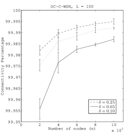
(a)

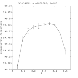
(b)

Figure 1: Weak radius: Percentage of sensors in the largest connected component in DC-C-WSN when LABEL:sub@fig:weak-condition-DC-C-WSN-varN $n$ varies, or LABEL:sub@fig:weak-condition-DC-C-WSN-varDELTA $\delta$ varies. The vertical bars represent the standard deviation.

Comparing this percentage with the percentage of sensors in the largest component when the radius of connectivity is the RGG radius in regular (i.e. all awake) wireless sensor networks (a radius that is $\frac{1}{\sqrt{\delta}}$ lower than the weak radius) we find that at the weak radius this percentage is from 5% to 10% higher (see Figure 2). In other words the weak radius is not a very useful theoretical result since we get a connectivity that is not that much higher than the connectivity at the RGG radius, but we have to transmit $1/\sqrt{\delta}$ times the distance. Indeed, on average since the power spent by each node in transmission is proportional to the square of the radius and since $n\delta$ sensors are awake in one time slot, the overall energy spent is almost the same as in regular WSNs, thereby negating the effect of duty-cycling.

This duty-cycling energy inefficiency is the second motivation that drove us to find a better theoretical result than that provided by the weak radius result of [7]. We now move on to presenting that better result.

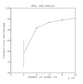
Figure 2: Percentage of sensors in the largest connected component for all awake WSNs adopting the lowest possible radius for connectivity, i.e., the RGG radius.

6.4 Optimal connectivity condition

Let now concentrate on the strong connectivity result that leads to the optimal radius, that is the radius $r(n)$ that satisfies Theorem 5.4. To compute the optimal radius for the contiguous and random duty-cycle scheme, we need to compute the probability $\gamma$ for each of them in the VB-RGG model.

In DC-C-WSNs, a sensor $v$ will share at least one slot with node $u$ if $v$ chooses as its starting point any of the slots $i_{u}-(d-1)\bmod L,\ldots,i_{u},\ldots i_{u}+(d-1)\bmod L$. Hence, two sensors have probability $\gamma=\frac{2d-1}{L}$ of sharing a slot. Now, let the optimal DC-C-WSN radius be the radius $r(n)$ that satisfies Theorem 5.4 when $\gamma=\frac{2d-1}{L}$. We have:

Corollary 6.1

When $\gamma=\frac{2d-1}{L}<1$, $\mbox{P}(\mbox{DC-C-WSN}\$ $\mbox{ is connected})\rightarrow 1$ as $n\rightarrow\infty$ if and only if

$$r(n)=\sqrt{\frac{\log n+c(n)}{(2\delta-1/L)\pi n}},$$ (25)

where $c=\lim_{n\rightarrow\infty}c(n)=\infty$.

Note that if $\gamma=\frac{2d-1}{L}>1$, the radius in (25) goes below the RGG radius and is no longer meaningful. However, $\gamma=\frac{2d-1}{L}>1$ implies $\delta>1/2$, and by Fact 3.1 the RGG radius given in (1) guarantees the connectivity property.

In DC-R-WSNs, when a node $u$ has chosen $d$ slots, another node $v$ has $d$ possibilities to choose one slot in common with $u$ and the probability of doing that is at least $\delta$ each time. Hence, the probability that two sensors share one slot is $\gamma>\left(1-(1-\delta)^{d}\right)$. Therefore, by Theorem 5.4, the optimal DC-R-WSN  radius must satisfy:

Corollary 6.2

$\mbox{P}(\mbox{DC-R-WSN}\ \mbox{ is connected})\rightarrow 1$ as $n\rightarrow\infty$ if and only if

$$r(n)=\sqrt{\frac{\log n+c(n)}{(1-(1-\delta)^{d})\pi n}},$$ (26)

where $c=\lim_{n\rightarrow\infty}c(n)=\infty$.

We first study the size of the largest component under the optimal radius. In Figure 3 we plot the the percentage of sensors that belong to the largest component on the $y$-axis versus $n$ on the $x$-axis when $L=100$, $10^{5}\leq n\leq 10^{6}$, $\delta=0.05,0.15$ and $0.25$. For both schemes, fixing a value of $\delta$, the size of the largest connected component increases when $n$ increases. In both DC-R-WSN and DC-C-WSN we note that the percentage of nodes in the largest component decreases as $\delta$ increases, which is expected since $\gamma$ increases as $\delta$ increases and so the optimal radius decreases (see Table 2 for more details). Nonetheless, for all the experiments on DC-C-WSNs, more than 90% of the sensors belong to the largest component. This is also true for DC-R-WSNs for small values of $\delta$ and even for larger values of $\delta$ for large enough $n$ (see Figure 3b). The substantial drop off in the size of the largest component of DC-R-WSN for $\delta=0.25$ is due to the fact that $\gamma$ rises very quickly to 1 in this case and so the optimal radius of DC-R-WSN falls quickly down to the RGG radius (see Table 2).

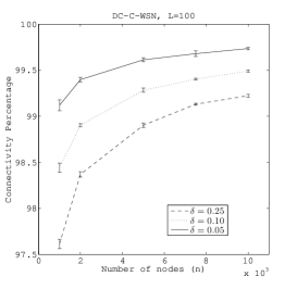
(a)

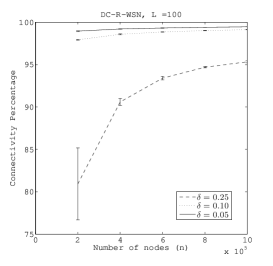
(b)

Figure 3: Optimal radius: Percentage of sensors in the largest connected component for different values of $\delta$ when $n$ varies LABEL:sub@fig:strong-n-condition-DC-C-WSN in DC-C-WSN LABEL:sub@fig:strong-n-condition-DC-R-WSN in DC-R-WSN.

	$L=200$		$L=100$
$\delta$	DC-C-WSN	DC-R-WSN	DC-C-WSN	DC-R-WSN
0.02	1.322	1.970	1.224	1.407
0.05	1.378	2.832	1.341	2.127
0.10	1.396	2.963	1.378	2.552
0.15	1.402	2.572	1.390	2.466
0.20	1.405	2.236	1.396	2.249
0.50	1.410	1.414	1.407	1.414

Table 1: The ratio between the weak and the optimal radius in DC-C-WSN and DC-R-WSN for different $\delta$ and $L$.

We tabulate in Table 1 the ratio of the weak and optimal radii in both schemes to explain Figures 1 and  3. We note that whereas the weak radius is the same for both DC-C-WSN and DC-R-WSN whenever $\delta$ is fixed, there is a radical difference in the optimal radius. observe that as suggested by (25), for DC-C-WSN the weak radius is approximately a $\sqrt{2}$ factor longer than the optimal radius. Such a factor decreases when the cycle length $L$ decreases, but it remains always below $\sqrt{2}$. For DC-R-WSN in contrast when $0.05\leq\delta\leq 0.4$ and $d>4$, the ratio between the weak and the optimal radius is always above $\sqrt{2}$, implying that DC-R-WSNs require a smaller transmission radius to be connected than the DC-C-WSNs. We also note that the ratio is consistently higher for DC-R-WSN although as $\delta$ reaches 0.5 the ratio becomes about the same since $\gamma$ reaches close to 1 for both schemes.

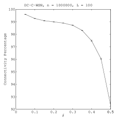
(a)

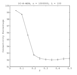
(b)

Figure 4: Optimal radius: Percentage of sensors in the largest connected component when $\delta$ varies, $n$ and $L$ are fixed in LABEL:sub@fig:strong-delta-fixNL-connectivity-DC-C DC-C-WSNs LABEL:sub@fig:strong-delta-fixNL-connectivity-DC-R DC-R-WSNs.

Figure 4 depicts the connectivity percentage of DC-C-WSNs and DC-R-WSNs under the optimal radius when $n=10^{6}$, $\delta$ varies in $[0.1,0.5]$ and $L$ is fixed to $100$. We see that as $\delta$ increases up to $0.15$, the optimal radius in DC-R-WSNs decreases fast towards the RGG radius, and so the connectivity of DC-R-WSNs in Figure 4b decreases. Past this point, i.e. for larger values of $\delta$, the optimal radius is close to the RGG radius and the connectivity in DC-R-WSNs remains stable and substantially close to that of regular sensor networks. In Figure 4a the connectivity remains stable and 5% above that of regular sensors as expected since the optimal radius is approximately $3/2$ times the RGG radius and decreases slowly. Clearly, it appears that, for both schemes, the connectivity performance decrease happens when the radius approaches the RGG radius model, but the performance is never worse than that of regular networks.

This observation is backed up by Table 2 where the weak and the optimal radius are compared with the minimum possible radius given by the RGG model for two different values of $L$.

	$L=200$		$L=100$
$\delta$	DC-C-WSN	DC-R-WSN	DC-C-WSN	DC-R-WSN
0.02	5.345	3.589	5.773	5.025
0.05	3.244	1.578	3.333	2.102
0.10	2.264	1.067	2.294	1.239
0.15	1.841	1.003	1.857	1.046
0.20	1.591	1.000	1.601	1.005
0.50	1.002	1	1.005	1.005

Table 2: The ratio between the optimal radius and the minimum possible transmission radius (i.e, the RGG radius).

We also studied the influence of $L$ on the percentage of connectivity in Figure 5. Here we fix $d$, while $L$ changes accordingly to $d/\delta$. One immediately notes that the drop off in DC-R-WSNs is less than the drop off in Figure 4. In the case of DC-R-WSNs, this different behaviour is due to the fact that, as reported in Table 3, the optimal radius for the DC-R-WSNs decreases slower when $L$ is fixed than when $d$ is fixed. For DC-C-WSNs, the variation of the optimal radius when $\delta$ changes and either $d$ or $L$ are fixed is minimal showing that DC-C-WSNs are less influenced by $L$. To be precise, the optimal radius when $d=5$ is slightly greater than when $L=100$ and so is the connectivity, which remains above 97% even when $\delta=0.5$.

(a)

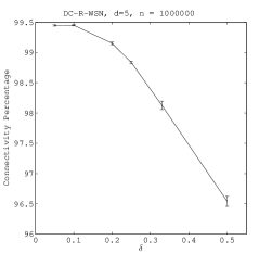
(b)

Figure 5: Optimal radius: Percentage of sensors in the largest connected component when $\delta$ varies, $n$ and $d$ are fixed in LABEL:sub@fig:strong-delta-fixNd-connectivity-DC-C DC-C-WSNs LABEL:sub@fig:strong-delta-fixNd-connectivity-DC-R DC-R-WSNs.

	DC-C-WSNs		DC-R-WSNs
$\delta$	$d=5$	$L=100$	$d=5$	$L=100$
0.05	3.333	3.333	2.102	2.102
0.10	2.357	2.294	1.562	1.239
0.20	1.667	1.601	1.219	1.005
0.40	1.178	1.125	1.042	1

Table 3: The ratio between the optimal radius and the minimum possible transmission radius (i.e, the RGG radius) when $\delta$ varies and either $d$ or $L$ are fixed.

We now show that under the strong connectivity condition, the energy saving is effective. On average, DC-C-WSNs spend half the energy of the regular WSNs since there are $n\delta$ awake sensors and each sensor transmits with energy proportional to $\frac{1}{2\delta}$ times the energy spent by a sensor in an always-awake WSN. A higher saving is possible for DC-R-WSNs. In fact, each awake sensor transmits with energy proportional to the energy spent by a sensor in an always awake WSN multiplied by $\frac{1}{1-(1-\delta)^{d}}\approx\frac{1}{1-e^{-d\delta}}$, which becomes very close to $1$ when $\delta>0.20$. Hence, DC-R-WSNs spend energy proportional to the number $n\delta$ of awake sensors, which is the most desirable situation. In conclusion, the optimal connectivity condition undoubtedly leads to a great gain in the radius length, and thus leads to a great energy saving in power transmission for both schemes, but especially for DC-R-WSNs.

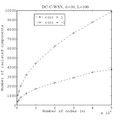
(a)

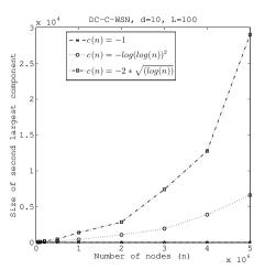
(b)

Figure 6: LABEL:sub@fig:cc1-1 The number of isolated points in DC-C-WSN. LABEL:sub@fig:largestsecond The size of the largest second component in DC-C-WSNs.

To establish that the radius condition given in Corollary 6.1 is necessary we studied the situation where $c(n)$ does not grow to $\infty$ as $n$ grows (Figure 6). Figure 6a shows that although the connectivity is still high in DC-C-WSN when $c(n)=1$ and when $c(n)=-1$, the number of isolated nodes is rapidly increasing, the increase being faster in the case where $c(n)=-1$. This indicates that the percentage connectivity is continuously dropping. Moreover, Figure 6b shows that when $c(n)<0$, the size of the second largest component increases as $|c(n)|$ increases which implies that the probability of connectivity tends to 0 as $n\rightarrow\infty$ if $\lim_{n\rightarrow\infty}c(n)=-\infty$. These results show the necessity of the condition on $c(n)$.

We conducted a series of experiments to establish the optimality of the optimal radius. In particular, we varied the additive factor $c(n)$ in the optimal connectivity condition. As we expect from the previous discussion, since the optimal DC-R-WSN radius falls more sharply than the optimal radius for DC-C-WSN (and in fact is not far from the minimum RGG radius), the connectivity in DC-R-WSNs drops before it does in DC-C-WSNs. Figure 7 shows that when $c(n)=-\log\log(n)$ DC-R-WSNs are below 10% of connectivity independent of $n$, while DC-C-WSNs still reach a good percentage of connectivity, especially for large $n$. Figure 8 shows for which values of $c(n)$ both schemes experience a comparable and drastic loss of connectivity, dropping below $0.2$%. For DC-C-WSNs, this happens between $c(n)=-(\log{\log{n}})^{2}$ and $c(n)=-2\sqrt{\log{n}}$ (see Table 4 for the absolute values), while for DC-R-WSNs this happens when $c(n)=-5$.

	$c(n)$
n	-$(\log\log n)^{2}$	-2*$\sqrt{\log n}$	-2.5*$\sqrt{\log n}$
$0.5*10^{6}$	-6.60	-5.25	-6.57
$10^{6}$	-6.86	-7.43	-9.29
$1.5*10^{6}$	-7.02	-9.10	-11.38
$2*10^{6}$	-7.12	-10.51	-13.14
$2.5*10^{6}$	-7.23	-11.75	-14.69

Table 4: The values of $c(n)$ when $n$ varies.

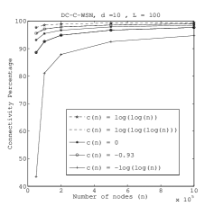
(a)

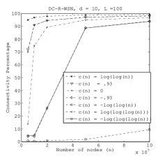
(b)

Figure 7: Percentage of connectivity LABEL:sub@fig:percentage-constant-DC-C in DC-C-WSN LABEL:sub@fig:percentage-constant-DC-R in DC-R-WSN.

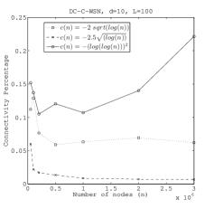
(a)

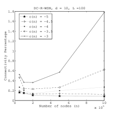
(b)

Figure 8: Percentage of connectivity with different values of $c(n)$ in LABEL:sub@fig:constant-DC-C DC-C-WSNLABEL:sub@fig:constant-DC-R DC-R-WSN.

6.5 Power consumption in DC-C-WSNs and DC-R-WSNs

The main focus of this paper is to study the minimum radius that guarantees connectivity of the duty-cycling graph for a large family of duty-cycling schemes, i.e. to study the minimum local transmission power spent by a duty-cycled sensor. It is not clear that minimizing local power leads to minimum global power consumption for any given set of packets being sent across the network. We do not attempt any comprehensive characterization of the power consumption of different routing problems in the duty-cycled case since that is outside the scope of this paper. Instead we pick a simple point-to-point communication task and compare the power consumption of the weak and optimal radii of DC-R-WSN and DC-C-WSN for that task. We also study the power consumption of the “always on” network that uses the RGG radius to connect which corresponds to a local power level that is lower than the local power levels of the duty-cycled networks we study.

Simulation setup

In the experiments related to global power consumption, we use the sensor power consumption levels given in Table 5 [25, 6]. To calibrate our experiments we set $P=50mW$ as the power spent for transmitting up to the RGG radius $r(n)$ (see Equation 1) with $n=2*10^{5}$ and $c(n)=\log\log n$. The transmission power $P(\overline{r}(n^{\prime}))$ to cover an arbitrary radius $\overline{r}(n^{\prime})$ is then given by $P(\overline{r}(n^{\prime}))=P(r(n))\cdot\frac{\overline{r}^{2}(n^{\prime})}{r^{2}(n)}$. Note that the radius $\overline{r}(n^{\prime})$ varies according to the duty-cycle scheme and the number of sensors. Moreover, since the transmission is considered successful if the SINR (Signal-to-Interference-plus-Noise-Ratio) is above a certain threshold, we assume that the power for receiving $M$ is independent of the distance between the transmitting and the receiving sensor.

Table 5: Estimate of sensor power consumption in different operational modes at $2.5$ Volt and with a sensor RGG transmission radius $r(n)=\sqrt{\frac{\log n+\log\log n}{n}}$ and $n=2*10^{5}$.

Sensor Mode	Current Drawn	Power Consumed
Sleep
(CPU inactive, timer on, radio off)	6 $\mu A$	0.015 $mW$
CPU switch on, radio startup	3 $mA$	15 $mW$
CPU switch off, radio shutdown	3 $mA$	15 $mW$
Awake
(CPU active, radio listening or RX)	12 $mA$	32 $mW$
CPU active, radio TX	20 $mA$	50 $mW$

We assume that if a sensor is awake, the CPU is active and the sensor listens to the radio. In this way, awake sensors can receive the incoming message $M$ without extra overhead [25]. Moreover, we do not consider interference in our simplified simulations. Power is also spent to switch between sleep and awake modes, i.e., to switch on/off both the CPU and the radio. Note that, in this model, the only extra power for performing any network task is the power spent in actually transmitting packets which is directly proportional to the square of the current transmission radius. We will see ahead that the power consumed by transmissions in our network task is the least in the “always on” case which is expected since the radius of transmission is the lowest. But, the power required to operate the network in the “always on” case is much higher. For example, a simple calculation shows that over 100 times slots the “always on” network consumes 3.2 W per node only for operation without any transmission. On the other hand for the duty-cycled case, setting $\delta=0.05$ and $L=100$ i.e. with $d=5$, assuming one transition from sleep to waking and one from waking to sleep in the DC-C-WSN case we find that the total power consumed at a node is 0.19W which is 16 times lower than the “always on” case. Since in DC-R-WSN the number of transitions between sleep and waking are more the power consumed is slightly higher but is no more than 0.31W (counting five transitions from sleep to wake and five in the opposite direction) which is more than 10 times lower than the “always on” case. Therefore we see an order of magnitude difference in the operation of the network that more than compensates (as we will see) for the extra power spent in transmission in most network tasks.

The network task

The network operation we will study, $\mbox{Send}(M,S,D)$ involves sending message $M$ from source node $S$ to destination node $D$. We define the total transmission power of this operation as the sum of the power spent in transmission only by each sensor that receives and retransmits $M$ during the broadcast operation. We experimentally measure by simulations the total transmission power for the two concrete DC-C-WSN and DC-R-WSN schemes when the weak and the optimal radius are used. We also consider the total transmission power for $\mbox{Send}(M,S,D)$ on always awake WSNs, where each sensor transmits adopting the RGG radius. The results presented, unlike our previous results in Theorems 4.1 and  5.4, have no general validity. We claim them only for the two specific duty-cycling schemes we have studied so far, and that too only for the operation $\mbox{Send}(M,S,D)$.

In our experiments, we select the source $S$ for the $\mbox{Send}(M,S,D)$ operation in the center of the deployment area, which is a disk of unit radius, and the destination $D$ is an arbitrary sensor at Euclidean distance $d(S,D)=0.1$ from $S$. We assume that each sensor knows its polar coordinates in the deployment.

In order to a simulate realistic situation we implement $\mbox{Send}(M,S,D)$ using a greedy algorithm which is a kind of partial flooding of the network as follows:

1. $S$ sends the message $M$ to all its neighbors.

2. Node $u$ retransmits $M$ only the first time it receives the message under the following condition: u transmits M for d slots (i.e. for one duty-cycle) if it receives from a sender v which is further from D than u itself.

We call this algorithm the greedy directional algorithm since it tries to move the message in the direction of the destination i.e. the distance between transmitting sensor and $D$ is guaranteed to decrease as the hop count of the message increases. We also implement a relaxed greedy directional (or simply, relaxed greedy) algorithm which is the same as the greedy directional algorithm except that a sensor retransmits $M$ if its Euclidean distance from $D$ is no larger than $1.2$ times the distance of the sender i.e. in the relaxed greedy algorithm, the distance between the transmitting sensor and $D$ is not guaranteed to decrease at every hop, although it increases by a bounded amount

Whenever not otherwise specified, $\mbox{Send}(M,S,D)$ is implemented by the greedy directional algorithm. We use the relaxed greedy for the cases where greedy directional does not find a path (despite the network being connected) e.g. in the “always on” case that uses the RGG radius and DC-R-WSN when it uses the optimal radius. The failure of the greedy to find a path in these situations is due to the fact that since the radii here are very low, the paths from $S$ to $D$ can sometimes encounter twists and turns and may not always move in the desired direction.

Results and analysis

To contextualize the power consumption of $\mbox{Send}(MSD)$ we began by plotting the number of hops needed to complete the task under the DC-R-WSN and DC-C-WSN with both the optimal radius and the weak radius, as well as the number of hops needed by the “always on” network using the RGG radius (Figure 9a). Additionally we plotted the number of time slots taken to complete the task in the five cases considered above (Figure 9b). We found that the number of hops increases more or less as the radius decreases, with the RGG scheme having the maximum number hops. Although the weak radius is the same for DC-C-WSN and DC-R-WSN  the number of hops to reach $D$ is smaller in the latter case because of the greater probability of connection in DC-R-WSN. We find that for the duty-cycled schemes the completion times report in Figure 9b are in the same order as the number of hops i.e. lower the number of hops for a scheme, the quicker the message reaches the destination. The RGG scheme has a much lower completion time than the duty-cycled schemes, which is to be expected since sensors are always on in this case.

(a)

(b)

Figure 9: When $\delta=0.05$, $L=100$ and $d=5$: LABEL:sub@fig:1_hops Number of hops to reach $D$ from $S$ LABEL:sub@fig:4_timer Total completion time for $\mbox{Send}(M,S,D)$.

Figure 10: Number of sensors that receive $M$ and retransmit it during the $\mbox{Send}(M,S,D)$ operation when $\delta=0.05$.

Figure 10 plots the number $N^{\prime}$ of sensors that receive $M$ and retransmit it during the $\mbox{Send}(M,S,D)$ operation from $S$ to $D$. In general $N^{\prime}$ increases with the number of hops with the “always on” sensors registering the highest values of the five scenarios studied. When the radius is the same for both DC-C-WSN and DC-R-WSN, i.e. the weak radius, we find that $N^{\prime}$ is larger for DC-R-WSN although we had seen in Figure 9a that number of hops for DC-R-WSN with weak radius is lower than that of DC-C-WSN with weak radius. Here we see that a node’s ability to make more connections under the DC-R-WSN scheme becomes a disadvantage in terms of power consumption.

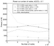
(a)

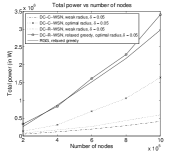
(b)

Figure 11: For $\mbox{Send}(M,S,D)$, when $d(S,D)=0.1$, $\delta=0.05$, and $L=100$: LABEL:sub@fig:3_diff Total transmission power LABEL:sub@fig:7_power Total power consumed in task.

Figure 11a plots the total transmission power, i.e. the power spent only in transmission by all the sensors that participate in $\mbox{Send}(M,S,D)$. Among the duty-cycled schemes the winner here is DC-C-WSN with optimal radius which reflects the fact that it has a low number of transmitting nodes $N^{\prime}$. The DC-R-WSN schemes both perform worse than the DC-C-WSN schemes which is a clear consequence of having made a larger number of transmissions (as we saw in Figure 10). But, on the other hand, DC-R-WSN with optimal radius beats DC-R-WSN with weak radius, despite having made more transmissions which shows the benefit of having a lower local power consumption. Always awake WSNs spend very little amount of energy for transmission, but, as we see in Figure 11b, the total power they consume to complete the task is among the highest which is clearly a consequence of their high cost of operation. We note in Figure 11b that the duty-cycled networks that adopt the weak radius are those that consume the minimum total power. Among these the DC-C-WSNs demand less power networks since they need lower transmission power, as seen in Figure 11a, and because they consume less power for their basic operation since they just switch once between sleep and awake mode in each period. Overall the worst performer is DC-R-WSN with the optimal radius which is due to the fact that the poor connectivity it offers forces us to use the relaxed greedy algorithm, thereby incurring a greater number of transmissions (as we saw in Figure 10) that offsets the benefit of the low power consumption in local transmissions.

In conclusion we see that the global power consumption for a given network task depends on several factors, many of which are specific to the task that we are attempting. Minimizing the local power consumption does not automatically minimize the global power consumption for a given task. However the low cost of basic operation of duty-cycled networks benefits them as long as they offer good connectivity that allows us to carry out the given task.

7 A minimum-radius duty-cycling scheme

So far we have studied the situation where given $d$ and $L$ and some scheme for selecting $d$ waking slots out of $L$ we have a probability $\gamma$ for connection between two neighboring nodes and hence a minimum transmission radius for achieving connectivity in the network. This transmission radius is $1/\sqrt{\gamma}$ higher than the radius required for connectivity in RGGs. Now we show that with a careful choice of such a scheme for selecting the slots we can achieve connectivity even at the RGG radius. Namely, in this section we move away from the general approach spanning a whole family of duty-cycling schemes of the previous section and give an algorithm for finding a particular awake scheduling scheme that ensures that the duty-cycled network achieves connectivity using the RGG radius.

Given an integer $k>1$, consider a duty cycling scheme with the following properties:

1. Each node chooses a duty cycle from one of $k$ predefined options, we call them $C_{1},\ldots,C_{k}$ where each $C_{i}\subseteq\{0,1,\ldots,L\-1\}$ and $|C_{i}|=\delta\cdot L=d$.

2. All $k$ duty-cycle options overlap i.e. for each $1\leq i\neq,j\leq k$, $C_{i}\cap C_{j}\neq\emptyset$.

3. No time instance is left uncovered i.e. $\cup_{i=1}^{k}C_{i}=\{0,1,\ldots,L-1\}$.

Note that if such a scheme were to exist, we would be able to send data from any node to node provided the base network is connected i.e. if the Gupta-Kumar bound is satisfied (without any extra factor) we achieve connectivity, since a node with any of the $k$ duty-cycles can send a message to any of its neighbors. It just has to wait for the overlap point of time to come. Also, from a time coverage point of view this scheme is good since there is no point of time when all the sensors are off. And, in fact, on average $1/k$ fraction of all sensors at least are guaranteed to be on at any time step.

The question is: Does such a schedule exist? The answer is yes. Consider the following simple definition of a schedule:

Given $k$ we build $k$ schedules $A_{1},\ldots A_{k}$ by randomly picking $d$ time slots for each one of them independently of the others.

Clearly if $\delta>1/2$ then any $k$ duty cycles we choose have the property that all of them overlap, so we focus on the case where $\delta\leq 1/2$.

Claim 7.1

For a given $k$, the random selection schedule described above has the property that all the $k$ schedules overlap, with probability at least

$$1-\frac{k(k+1)}{2}\cdot e^{-\delta d}.$$

Proof.  The probability that two schedules $A_{i}$ and $A_{j}$ do not overlap is computed by calculating the probability that $A_{j}$ is picked only from $\{0,1,2,\ldots,L-1\}\setminus A_{i}$ i.e.

$$\mbox{P}(A_{i}\cap A_{j}=\emptyset)={L-d\choose d}/{L\choose d}=\frac{L-d\cdot(L-d-1)\cdots(L-2d+1)}{L\cdot(L-1)\cdots(L-d+1)}\leq\left(1-\frac{d}{L}\right)^{d}\leq e^{-\delta d}.$$

Since there are $k(k+1)/2$ such pairs, we get the result claimed. $\sqcap$$\sqcup$

We turn to the time coverage property. Clearly, the probability that a given slot $i$, $0\leq i<L$ is not covered by a given schedule is $(1-\delta)$. Since all the schedules are independent, slot $i$ is not covered by any schedule is $(1-\delta)^{k}$. Hence, using the union bound over all the $L$ slots, we get:

Claim 7.2

The probability that every time slot is covered by at least one schedule is at least

$$1-L\cdot e^{-\delta k}.$$

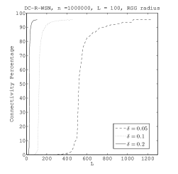
Figure 12: Connectivity Percentage in a deterministic duty-cycle scheme when $L$ and $\delta$ vary.

Hence we get that a random choice of the $k$ duty-cycle schedules gives us a schedule with both properties with probability:

$$1-\left(\frac{k(k+1)}{2}\cdot e^{-\delta d}+L\cdot e^{-\delta k}\right).$$

This probability can be made arbitrarily close to 1 by choosing $L$ large enough and setting $k$ to a value that is $\theta(\log L)$. But even if this probability is non-zero that is fine, because we need to find these schedules offline and then hard code them into the sensors. So, a randomized algorithm that keeps selecting $k$-schedules and then testing them to see if they have both properties will finish in polynomial time with high probability since testing for the two properties can easily be done in linear time.

Hence, we see that there is a way of organizing duty-cycles for any given value of $\delta$ such that if the Gupta-Kumar bound is achieved then connectivity if achieved. The parameter whose value suffers to achieve this is $L$ which may have to be made large. In Figure 12, the percentage of connectivity is plotted when $L$ and $\delta$ vary. For example, for $\delta=0.05$, the 90% of connectivity is reached for $L\geq 600$ and hence $d=30$ is a good choice for the deterministic duty-cycle scheme.

8 Conclusion: The wider implications of our results

In this paper we have studied the duty-cycled wireless sensor network setting and provided a necessary and sufficient condition on the radius of transmission for connectivity in such networks. The work we built on [7] provided only a sufficient condition which was a shortcoming that we have rectified. In the process we have defined a new random connection model which has not, to the best of our knowledge, been proposed earlier. The most important contribution of this paper is Theorem 5.4 which is a general theorem with implications beyond the duty-cycling setting.

An important setting in which Theorem 5.4 is applicable is in wireless network security, specifically key-predistribution for secure communication. In this setting, Eschenauer and Gligor proposed a scheme in which each node of the network chooses $K$ keys at random from a pool of $P$ available keys, and secure communication is possible if two nodes share a common key [9]. Clearly if these nodes are part of a sensor network with limited transmission power at each node, the question of the radius of connectivity arises. It is also fairly clear that the model here is exactly similar to that of our random selection duty cycle with $P$ playing the role of $L$ and $K$ playing the role of $d$.

In fact, in a recent paper [28] it was pointed out that K. Krzywdziński and K. Rybarczyk [17] had proved that if

$$\pi r(n)^{2}\cdot\alpha_{n}=c\frac{\log n}{n},$$

where $\alpha_{n}$ is the probability of two nodes sharing a key (corresponding to $\gamma$ in our case), then the random geometric graph with the Eschenauer-Gligor scheme is connected with probability tending to 1 if $c>8$ and is disconnected with probability tending to 1 if $c<1$. In [28] the author also claims that Yi. et. al. [33] had conjectured a stronger result on the lines of Gupta and Kumar’s result  [13], i.e. the Eschenauer-Gligor scheme on a graph is connected with probability tending to 1 if and only if

$$\pi r(n)^{2}\cdot\alpha_{n}=\frac{\log n+c(n)}{n},$$

and $c(n)\rightarrow\infty$ as $n\rightarrow\infty$. This conjecture (Eq. (3) in [28]) can now be considered closed since it is nothing other than our Corollary 6.2 which, as we have seen, follows easily from Theorem 5.4. It is our belief that for the more abstract problem of key-predistribution on a complete graph (see e.g. [29]), our method of defining a vertex-based model of connectivity and proving the requisite properties may help improve the current best known results in that area as well.

We feel that as in the case of key-predistribution on RGGs, there may be other settings where Theorem 5.4 may be applicable, for example the study of connectivity in WSNs with directional antennas where the direction is fixed at random independently at each node. Our contribution, therefore, is a general and foundational contribution, as well as a detailed and in-depth study of the particular setting of duty-cycled WSNs.

APPENDIX

Appendix A Proof of Lemma 5.3

In order to prove this theorem we will show that Penrose’s proof technique can be followed for our model as well. To show this we define some notation first defined in [22].

Suppose $U=\{x_{1},\ldots,x_{k}\}$ is finite set of points in $\mathbb{R}^{2}$ and $x_{0}$ is another point in $\mathbb{R}^{2}$. Suppose we form a random graph $G$ with the points $U\cup\{x_{0}\}$ using our connection function $g(\cdot,\cdot)$ i.e. we associate a copy of $Z$ with each of the points and then draw edges as defined in (5).

• Define $g_{1}(x_{0};U)$ to be the probability that $x_{0}$ is not isolated in this graph i.e. that $x_{0}$ is connected to at least one of the points in $U$.

• Also define $g_{2}(x_{0},x_{1},\ldots,x_{k})$ to be the probability that the graph $G$ is connected.

The proof technique partitions the event $\{|W|=k\}$ by mapping the points of $W$ to a lattice of points of the form $\delta z,z\in\mathbb{Z}^{2}$ and studying the number of such points in the mapping. This is done as follows: We define a map $F_{\delta}:\mathbb{R}^{2}\rightarrow\delta\mathbb{Z}^{2}$ which sends a point of $\mathbb{R}^{2}$ to the nearest point of the lattice $\delta\mathbb{Z}^{2}$. Since in general there may be more than one such point, we note that in a Poisson point process this does not happen with probability 1, and hence this map is well defined with probability 1. What could happen, however is that a number of points of $\mathbb{R}^{2}$ get mapped to the same point of $\delta\mathbb{Z}^{2}$ and in fact we can see that a box of width $\delta$ centred at a point of the lattice is mapped to the lattice point at the centre by $F_{\delta}$. To be able to describe such boxes, we denote by $B_{l}$ the box $[-l,l]\times[-l,l]$ i.e. the box of width $2l$ centred at the origin. Further we will denote by $S_{\delta}$ the set of points of $\delta\mathbb{Z}^{2}$ which are images of the points in $W$.

In order to prove the theorem, we will prove the following lemmas that Penrose demonstrated are true for the random connection model.

Lemma A.1

For sufficiently small $\delta$,

$$\lim_{\lambda\rightarrow\infty}\frac{\sum_{k=2}^{\infty}\mbox{P}_{\lambda}(|W|=k\cap|S_{\delta}|=1)}{q_{1}(\lambda)}=0.$$

This lemma is clearly not enough to prove Lemma 5.3, but it helps us prove the following lemma from which the theorem follows:

Lemma A.2

For sufficiently small $\delta$ and for each fixed $m$,

$$\lim_{\lambda\rightarrow\infty}\frac{\sum_{k=1}^{\infty}\mbox{P}_{\lambda}(|W|=k\cap|S_{\delta}|=m)}{q_{1}(\lambda)}=0.$$

We will need the following general characterization:

Proposition A.3

For any $k\in\mathbb{N}$,

$$\mbox{P}_{\lambda}(|W|=k\cap W\subset B_{l})= \frac{\lambda^{k-1}}{(k-1)!}\int_{B_{l}}\cdots\int_{B_{l}}g_{2}(0,x_{1},\ldots,x_{k}-1)$$

$$\cdot\exp\left\{-\lambda\int_{\mathbb{R}^{2}}g_{1}(y;\{0,x_{1},\ldots,x_{k-1})dy\right\}dx_{1}\cdots dx_{k-1}.$$ (27)

Proof.  Let $E(n,l)$ denote the event that $|W|=k$ and $W\subseteq B_{l}$. Let us condition on the event that the number of points of the Poisson process in $B_{l}$ is $m$, we call this event $|V(B_{l})|=m$. Recall that the $m$ points inside $B_{l}$ are uniformly distributed when we condition on $|V(B_{l})|=m$. Hence, we have that:

$$\mbox{P}(E(n,l)||V(B_{l})|=m)={m\choose k-1}\cdot\left(\frac{1}{2l}\right)^{2m}\cdot\int_{B_{l}}\cdots\int_{B_{l}}\mbox{P}^{\prime}(W=\{0,x_{1},\ldots,x_{k-1}\})dx_{1}\cdots dx_{k-1},$$ (28)

where $\mbox{P}^{\prime}(0,x_{1},\ldots,x_{k-1})$ is the probability measure in the subspace where there are $m$ uniformly distributed points in $B_{l}$, there is a point at the origin, and there is a Poisson point process of density $\lambda$ in $\mathbb{R}^{2}\setminus B_{l}$. The integral on the right hand side is obtained by conditioning on the events that each of the $m$ points is in a square of area $dx_{i},1\leq i\leq m$ (with probability $dx_{i}/(2l)^{2}$ and then choosing $k-1$ of them to be part of $W$. We decondition by integrating over $B_{l}$ for all $m$ points. The $m-(k-1)$ that don’t get chosen simply contribute a factor of $1/(2l)^{2}$ to the integral.

If $W=\{0,x_{1},\ldots,x_{k-1}\}$ then it must be the case that no point from $\mathbb{R}^{2}\setminus B_{l}$ is connected to the points $0,x_{1},\ldots,x_{l}$. We use the function $g_{1}(\cdot;\cdots)$ defined above in this case. As remarked above, given a fixed set of points, $0,x_{1},\ldots,x_{k-1}$ in this case, the collection of events that any point of $\mathbb{R}^{2}\setminus B_{l}$ is connected to (or isolated from) these points is an independent collection. Hence, by Proposition 1.3 of Meester and Roy [20], the set of points connected to these points forms an (inhomogeneous) thinning of the Poisson point process $V(\mathbb{R}^{2}\setminus B_{l}$, with a thinning factor which is exactly equal to $g_{1}(y;0,x_{1},\dots,x_{k-1})$ for any point $y\in\mathbb{R}^{2}\setminus B_{l}$. Hence, the probability that no point of $\mathbb{R}^{2}\setminus B_{l}$ is connected to any of $0,x_{1},\ldots,x_{k-1}$ is

$$\exp\left\{-\lambda\int_{\mathbb{R}^{2}\setminus B_{l}}g_{1}(y;0,x_{1},\dots,x_{k-1})dy\right\}.$$

From the definition of $g_{2}(\cdots)$ we obtain that

$$\mbox{P}^{\prime}(W=\{0,x_{1},\ldots,x_{k-1}\}) =g_{2}(0,x_{1},\ldots,x_{k-1})\cdot\exp\left\{-\lambda\int_{\mathbb{R}^{2}\setminus B_{l}}g_{1}(y;0,x_{1},\dots,x_{k-1})dy\right\}$$

$$\cdot\prod_{i=k}^{m}(1-g_{1}(x_{i};0,x_{1},\ldots,x_{k-1})),$$

where again we use the fact that the events that $x_{i}$ is isolated from $0,x_{1},\ldots,x_{k-1}$, for $k\leq i\leq m$ form an independent collection. Now, substituting into (28), we get

$$\mbox{P}(E(n,l)\cap|V(B_{l})|=m) =e^{-\lambda(2l)^{2}}\frac{(\lambda(2l)^{2})^{m}}{m!}{m\choose k-1}\cdot\left(\frac{1}{2l}\right)^{2m}$$

$$\cdot\int_{B_{l}}\cdots\int_{B_{l}}g_{2}(0,x_{1},\ldots,x_{k-1})$$

$$\cdot\exp\left\{-\lambda\int_{\mathbb{R}^{2}\setminus B_{l}}g_{1}(y;0,x_{1},\dots,x_{k-1})dy\right\}$$

$$\cdot\left(\int_{B_{l}}(1-g_{1}(z;0,x_{1},\ldots,x_{k-1}))dz\right)^{m-(k-1)}dx_{1}\cdots dx_{k-1}.$$ (29)

Now consider the quantity:

$$a_{m} =e^{-\lambda(2l)^{2}}\frac{(\lambda(2l)^{2})^{m}}{m!}{m\choose k-1}\cdot\left(\frac{1}{2l}\right)^{2m}\cdot\left(\int_{B_{l}}(1-g_{1}(z;0,x_{1},\ldots,x_{k-1}))dz\right)^{m-(k-1)}$$

$$=e^{-\lambda(2l)^{2}}\frac{\lambda^{m}}{(m-(k-1))!(k-1)!}\cdot\left(\int_{B_{l}}(1-g_{1}(z;0,x_{1},\ldots,x_{k-1}))dz\right)^{m-(k-1)}.$$

Summing $a_{m}$ over all $m\geq k-1$, we get

$$\sum_{i=k-1}^{\infty}a_{m}=\frac{e^{-\lambda(2l)^{2}}\lambda^{k-1}}{(k-1)!}\cdot\exp-\left\{\lambda\int_{B_{l}}(1-g_{1}(z;0,x_{1},\ldots,x_{k-1}))dz\right\}.$$

Combining this with (29), we get

$$\mbox{P}(E(n,l)) =\frac{e^{-\lambda(2l)^{2}}\lambda^{k-1}}{(k-1)!}\cdot\int_{B_{l}}\cdots\int_{B_{l}}g_{2}(0,x_{1},\ldots,x_{k-1})$$

$$\cdot\exp\left\{-\lambda\int_{\mathbb{R}^{2}\setminus B_{l}}g_{1}(y;0,x_{1},\dots,x_{k-1})dy\right\}\cdot\exp\left\{-\lambda\int_{B_{l}}g_{1}(y;0,x_{1},\dots,x_{k-1})dy\right\}$$

$$\cdot\exp\left\{\int_{B_{l}}dz\right\}$$

The result follows by observing that the last term is equal to $e^{\lambda(2l)^{2}}$. $\sqcap$$\sqcup$

We now move to the proof of the two lemmas.

Proof of Lemma A.1:  Denote by $q^{\delta}_{k}(\lambda)$ the quantity $\mbox{P}(|W|=k\cap|S_{\delta}|=1)$. Since the condition that $|S_{\delta}|=1$ is the same as saying that all the points of $W$ are contained in $B_{\delta/2}$ i.e. the box with width $\delta$ centred at the origin, we can use Proposition A.3 to say that

$$\frac{q_{k}^{\delta}(\lambda)}{q_{1}{\lambda}} =\frac{\lambda^{k-1}}{(k-1)!}\int_{B_{\delta/2}}\cdots\int_{B_{\delta/2}}g_{2}(0,x_{1},\ldots,x_{k}-1)$$

$$\cdot\exp\left\{-\lambda\int_{\mathbb{R}^{2}}g_{1}(y;\{0,x_{1},\ldots,x_{k-1})dy\right\}dx_{1}\cdots dx_{k-1}.$$

$$\leq\frac{\lambda^{k-1}}{(k-1)!}\int_{B_{\delta/2}}\cdots\int_{B_{\delta/2}}\exp\left\{-\lambda\int_{\mathbb{R}^{2}}g_{1}(y;\{0,x_{1},\ldots,x_{k-1})dy\right\}dx_{1}\cdots dx_{k-1}.$$

The second step following by the fact that the function $g_{2}(\cdot;\cdots)$ takes value at most 1. Now, consider a $\delta$ small enough that $B_{\delta}$ is completely contained in a circle centred at 0 with radius $r/2$, where $r$ is the radius defined in the connection function. Let us denote this circle $C(0,r/2)$. In order to apply the connection diversity condition we use the lower bound

$$\int_{\mathbb{R}^{2}}g_{1}(y;\{0,x_{1},\ldots,x_{k-1})dy\geq\int_{C(0,r/2)}g_{1}(y;\{0,x_{1},\ldots,x_{k-1})dy.$$

Clearly a point in $C(0,r/2)$ is within distance $r$ of any other point in $C(0,r/2)$, so we can apply the connection diversity condition (8) to get

$$\frac{q_{k}^{\delta}(\lambda)}{q_{1}{\lambda}} \leq\frac{\lambda^{k-1}}{(k-1)!}\int_{B_{\delta/2}}\cdots\int_{B_{\delta/2}}\exp\left\{-\lambda\int_{C(0,r/2)}cdy\right\}dx_{1}\cdots dx_{k-1}.$$

$$=\frac{(\lambda\cdot\delta^{2})^{k-1}}{(k-1)!}\cdot e^{-c\pi r^{2}/2}.$$

Summing over $k\geq 2$, we get

$$\frac{\sum_{k=2}^{\infty}q_{k}^{\delta}(\lambda)}{q_{1}{\lambda}} \leq e^{-c\pi r^{2}/2}.\sum_{k=2}^{\infty}\frac{(\lambda\cdot(\delta)^{2})^{k-1}}{(k-1)!}$$

$$=e^{\lambda\delta^{2}-c\pi r^{2}/2},$$

Which tends to 0 as $\lambda\rightarrow\infty$ for all $\delta$ satisfying $\lambda\delta^{2}-c\pi r^{2}/2<0$. $\sqcap$$\sqcup$

Proof of Lemma A.2:  Since our connection function allows no connection beyond a fixed length (the so-called “bounded support” condition), there are only finitely many configurations of $S_{\delta}$ with $|S_{\delta}|=m$. So, we will show that for any $\eta$ which is a finite subset of $\delta\mathbb{Z}^{2}$,

$$\sum_{k=1}^{\infty}\mbox{P}_{\lambda}(|W|=k\cap S_{\delta}=\eta)/q_{1}(\lambda)\rightarrow 0\mbox{ as }\lambda\rightarrow\infty.$$

We denote by $W_{\eta}$, the connected component containing the origin when we remove all the points of $V$ that lie outside $F^{-1}_{\delta}(\eta)$ i.e. the area of the plane outside the set of squares of side $\delta$ depicted in Figure 13

Figure 13: $F_{\delta}$ with each point shown surrounded by a box of the form $B_{\delta/2}$. $A_{l}$, $A_{r}$ and $A_{t}$ are also shown.

Let $E(\eta,k)$ be the event that $W_{\eta}$ has $k$ points in it and for each point of $\eta$ at least one point of $W_{\eta}$ lies in the square of side $\delta$ centred at that point. Let $H_{\eta}$ be the event that there is no point of $V$ in $\mathbb{R}^{2}\setminus F^{-1}_{\delta}(\eta)$ that is connected to any point of $W_{\eta}$. Then the event $\{|W|=k\cap S_{\delta}=\eta\}$ is the same as the event $E(\eta,k)\cap H_{\eta}$. We will estimate the probability

$$\mbox{P}_{\lambda}(H_{\eta}|E(\eta,k))=\exp\left\{-\lambda\int_{\mathbb{R}^{2}\setminus F^{-1}_{\delta}(\eta)}g_{1}(y;W_{\eta})dy\right\}.$$ (30)

Where, as before, the equality follows from Proposition 1.3 of Meester and Roy [20]. Suppose we have $\delta_{1}$ small enough for the conclusion of Lemma A.1 to hold. In that case if $F^{-1}_{\delta}(\eta)$ can be contained in $B_{\delta_{1}/2}$ then the we are done. So we will assume that the width of $F^{-1}_{\delta}(\eta)$ is at least $\delta_{1}$. An argument symmetric to the one we will show can be made if the height is more than $\delta_{1}$.

Define $x_{l}=\inf\{x:(x,y)\in\eta\}$, $x_{r}=\sup\{x:(x,y)\in\eta\}$ and $x_{t}=\sup\{y:(x,y)\in\eta\}$ to be the $x$ coordinates of the leftmost and rightmost points, and the $y$ coordinate of the topmost points of $\eta$. Using these, define the sets $A_{l}=\{(x,y):x<x_{l}-\delta/2\}$, $A_{r}=\{(x,y):x<x_{l}+\delta/2\}$ and $A_{t}=\{(x,y):y>x_{t}+\delta/2,x_{l}-\delta/2\leq x\leq x_{r}+\delta/2\}$ (see Figure 13.) Note that $A_{l}$, $A_{r}$ and $A_{t}$ are disjoint regions of $\mathbb{R}^{2}\setminus F^{-1}_{\delta}(\eta)$.

By the definition of $E(\eta,k)$ and $x_{l}$, if $E(\eta,k)$ occurs there must exist a point $u_{1}=(x_{1},y_{1})\in W_{\eta}$ such that $|x_{1}-x_{l}|\leq\delta/2$. We lower bound the probability of a point in $A_{l}$ connecting to any point in $W_{\eta}$ by the probability that it connects to $u_{1}$. Hence

$$\int_{A_{l}}g_{1}(y,W_{\eta})dy\geq\int_{A_{l}}g(y,u_{1})dy$$

Since the distance between the boundary of $A_{l}$ and $u_{1}$ could be as large as $\delta$ (but not larger), and shifting $u_{1}$ to the origin, we have

$$\int_{A_{l}}g_{1}(y,W_{\eta})dy\geq\int_{(-\infty,-\delta)\times(-\infty,\infty)}g(y,0)dy$$

The same argument holds for $A_{r}$ with a similarly chose $u_{2}$ and so

$$\int_{A_{l}\cup A_{r}}g_{1}(y,W_{\eta})dy\geq\int_{\mathbb{R}^{2}}g(y,0)dy-\int_{(-\delta,\delta)\times(-\infty,\infty)}g(y,0)dy$$ (31)

Also, if $E(\eta,k)$ occurs, there is a point $u_{3}=(x_{3},y_{3})\in W_{\eta}$ such that $|x_{t}-y_{3}|\leq\delta/2$. And so, as before,

$$\int_{A_{t}}g_{1}(y,W_{\eta})dy\geq\int_{A_{t}}g(y,u_{3})dy$$ (32)

Now, we define two sets in $\mathbb{R}^{2}$, $A_{+}=(0,\delta_{1}/2)\times(\delta,\infty)$ and $A_{-}(-\delta_{1},0)\times(\delta,\infty)$. From the non-triviality condition on $f$ it is easy to see that for any value of $r>0$,

$$\min\left\{\int_{(0,\delta_{1}/2)\times(0,\infty)}g(0,x)dx,\int_{(-\delta_{1}/2,0)\times(0,\infty)}g(0,x)dx\right\}>0.$$

Hence, if we choose a small enough value of $\delta$, we can find a $c>0$ such that

$$\min\left\{\int_{A_{+}}g(0,x)dx,\int_{A_{-}}g(0,x)dx\right\}>c+\int_{(-\delta,\delta)\times(-\infty,\infty)}g(0,x)dx.$$ (33)

Note that $A_{-}$ and $A_{+}$ have width $\delta_{1}/2$ and we are in the case where the width of $\eta$ is at least $\delta_{1}$. So, if we recenter $A_{-}$ and $A_{+}$ at $u_{3}$, at least one of them will be fully contained in $A_{t}$. Combining this observation with (32) which bounds the integral of the isolation function in terms of the connection function around $u_{3}$ we get that

$$\int_{A_{t}}g_{1}(y,W_{\eta})dy\geq\min\left\{\int_{A_{+}}g(0,x)dx,\int_{A_{-}}g(0,x)dx\right\}$$

Further substituting (33), this given us

$$\int_{A_{t}}g_{1}(y,W_{\eta})dy\geq c+\int_{(-\delta,\delta)\times(-\infty,\infty)}g(0,x)dx.$$ (34)

Combining this with (31)

$$\int_{A_{t}\cup A_{l}\cup A_{r}}g_{1}(y,W_{\eta})dy\geq c+\int_{\mathbb{R}^{2}}g(0,x)dx.$$

Observing that $A_{l}\cup A_{r}\cup A_{t}\subseteq\mathbb{R}^{2}\setminus F^{-1}_{\delta}(\eta)$, the last equation substituted into (30) gives us that

$$\mbox{P}_{\lambda}(H_{\eta}|E(\eta,k))\leq\exp\left\{-\lambda\left(c+\int_{\mathbb{R}^{2}}g(0,x)dx\right)\right\}.$$

Since, $q_{1}(\lambda)=\exp\left\{-\lambda\int_{\mathbb{R}^{2}}g(0,x)dx\right\}$, we get that

$$\frac{\mbox{P}_{\lambda}(H_{\eta}|E(\eta,k))}{q_{1}(\lambda)}\leq e^{-\lambda c},$$

which in turn means that

$$\frac{\mbox{P}_{\lambda}(H_{\eta}\cap E(\eta,k))}{q_{1}(\lambda)}\leq\mbox{P}_{\lambda}(E(\eta,k))\cdot e^{-\lambda c}.$$

Summing over $k\geq 1$, we have

$$\frac{\sum_{k=1}^{\infty}\mbox{P}_{\lambda}(H_{\eta}\cap E(\eta,k))}{q_{1}(\lambda)}\leq e^{-\lambda c}\cdot\sum_{k=1}^{\infty}\mbox{P}_{\lambda}(E(\eta,k)).$$

For any fixed $\eta$, since $\sum_{k=1}^{\infty}\mbox{P}_{\lambda}(E(\eta,k))$ is at most 1, the right hand side tends to 0 as $\lambda\rightarrow\infty$. $\sqcap$$\sqcup$

References

- [1] N. Alon and J. H. Spencer. The probabilistic method. Wiley, 2nd edition edition, 2000.
- [2] G. Anastasi, M. Conti, M. D. Francesco, and A. Passarella. Energy conservation in wireless sensor networks: A survey. Ad Hoc Networks, 7(3):537–568, 2009.
- [3] A. Bagchi, C. M. Pinotti, S. Galhotra, and T. Mangla. Optimal radius for connectivity in duty-cycled wireless sensor networks. In Proc. 16th ACM Intl. Conf. on Modeling, Analysis and Simulation of Wireless and Mobile Systems (MSWIM ’13), pages 125–128, Barcelona, Spain, November 2013.
- [4] F. Barsi, A. A. Bertossi, C. Lavault, A. Navarra, S. Olariu, M. C. Pinotti, and V. Ravelomanana. Efficient location training protocols for heterogeneous sensor and actor networks. IEEE Trans. Mob. Comput., 10(3):377–391, 2011.
- [5] F. Barsi, A. A. Bertossi, F. B. Sorbelli, R. Ciotti, S. Olariu, and M. C. Pinotti. Asynchronous corona training protocols in wireless sensor and actor networks. IEEE Trans. on Parallel and Distributed Systems, 20(8):1216–1230, 2009.
- [6] A. A. Bertossi, S. Olariu, and C. M. Pinotti. Efficient corona training protocols for sensor networks. Theor. Comput. Sci., 402(1):2–15, 2008.
- [7] S. K. Das, A. Di Saverio, G. Ghidini, A. Navarra, and C. M. Pinotti. Broadcast analysis in dense duty-cycle sensor networks. In Proc. 6th International Conference on Ubiquitous Information Management and Communication (ICUIMC ’12), page article no. 16, New York, 2012. ACM.
- [8] P. Dutta, S. Dawson-Haggerty, Y. Chen, C.-J. M. Liang, and A. Terzis. Design and evaluation of a versatile and efficient receiver-initiated link layer for low-power wireless. In Proceedings of the 8th ACM Conference on Embedded Networked Sensor Systems (SenSys), 2010.
- [9] L. Eschenauer and V. D. Gligor. A key-management scheme for distributed sensor networks. In Proc. 9th Conference on Computer and Communications Security (CCS ’02), pages 41–47, New York, 2002. ACM.
- [10] G. Ghidini and S. Das. Energy-efficient markov chain-based duty cycling schemes for greener wireless sensor networks. J. Emerg. Technol. Comput. Syst., 8(4):29:1–29:32, 2012.
- [11] S. Guo, Y. Gu, B. Jiang, and T. He. Opportunistic flooding in low-duty-cycle wireless sensor networks with unreliable links. In Proceedings of the 15th annual international conference on Mobile computing and networking, pages 133–144. ACM, 2009.
- [12] P. Gupta and P. R. Kumar. Critical power for asymptotic connectivity. In Proc. 37th IEEE Conf. on Decision and Control, pages 1106–1110. IEEE, 1998.
- [13] P. Gupta and R. Kumar. Stochastic Analysis, Control, Optimization, and Applications: A Volume in Honor of W.H. Fleming, chapter Critical Power for Asymptotic Connectivity in Wireless Networks, pages 547–566. Springer, 1999.
- [14] K. Han, Y. Liu, and J. Luo. Duty-cycle-aware minimum-energy multicasting in wireless sensor networks. Networking, IEEE/ACM Transactions on, 21(3):910–923, 2013.
- [15] J. Hao, B. Zhang, and H. Mouftah. Routing protocols for duty cycled wireless sensor networks: A survey. Communications Magazine, IEEE, 50(12):116–123, 2012.
- [16] X. Jiao, W. Lou, J. Ma, J. Cao, X. Wang, and X. Zhou. Duty-cycle-aware minimum latency broadcast scheduling in multi-hop wireless networks. In Proceedings of the 30th IEEE International Conference on Distributed Computing Systems (ICDCS), pages 754–763. IEEE, 2010.
- [17] K. Krzywdziński and K. Rybarczyk. Geometric graphs with randomly deleted edges - connectivity and routing protocols. In Proc. 36th Intl. Symp. on Mathematical Foundations of Computer Science (MFCS 2011),, volume 6907 of Lecture Notes in Computer Science, pages 544–555. Springer, 2011.
- [18] S. Lai and B. Ravindran. Least-latency routing over time-dependent wireless sensor networks. IEEE Trans. Computers, 62(5):969–983, 2013.
- [19] G. Mao and B. Anderson. Connectivity of large wireless networks under a general connection model. IEEE Trans. Inf. Theory, 59(3):1761–1772, 2013.
- [20] R. Meester and R. Roy. Continuum Percolation. Number 119 in Cambridge Tracts in Mathematics. Cambridge University dss, Cambridge, 1996.
- [21] N. Pantazis and D. Vergados. A survey on power control issues in wireless sensor networks. Communications Surveys Tutorials, IEEE, 9(4):86–107, 2007.
- [22] M. D. Penrose. On a continuum percolation model. Adv. Appl. Probab., 23(3):546–556, September 1991.
- [23] J. Polastre, J. L. Hill, and D. E. Culler. Versatile low power media access for wireless sensor networks. In SenSys, pages 95–107, 2004.
- [24] S. Shakkottai, R. Srikant, and N. Shroff. Unreliable sensor grids: coverage, connectivity and diameter. In Proc. IEEE INFOCOM 2003, volume 2, pages 1073–1083. IEEE, 2003.
- [25] P. Shin, J. Park, and A. Kak. A predictive duty cycle adaptation framework using augmented sensing for wireless camera networks. ACM Trans. Sen. Netw., 10(2):22:1–22:31, Jan. 2014.
- [26] S. Sudevalayam and P. Kulkarni. Energy harvesting sensor nodes: Survey and implications. Communications Surveys Tutorials, IEEE, 13(3):443–461, 2011.
- [27] F. Wang and J. Liu. On Reliable Broadcast in Low Duty-Cycle Wireless Sensor Networks. IEEE Transactions on Mobile Computing, 11(5):767–779, 2012.
- [28] O. Yağan. Performance of the Eschenauer-Gligor key distribution scheme under an ON/OFF channel. IEEE Trans. Inf. Theory, 58(6):3821–3835, JUNE 2012.
- [29] O. Yağan and A. M. Makowski. Zero-one laws for connectivity in random key graphs. IEEE Trans. Inf. Theory, 58(5):2983–2999, May 2012.
- [30] W. Ye, J. S. Heidemann, and D. Estrin. An energy-efficient mac protocol for wireless sensor networks. In INFOCOM, 2002.
- [31] W. Ye, F. Silva, and J. Heidemann. Ultra-low duty cycle mac with scheduled channel polling. In Proceedings of the Fourth ACM SenSys Conference, pages 321–333, Boulder, Colorado, USA, November 2006. ACM.
- [32] C.-W. Yi, P.-J. Wang, X.-Y. Li, and O. Frieder. Asymptotic distribution of the number of isolated nodes in wireless ad hoc networks with Bernuolli nodes. IEEE Trans. Commun., 54(3):510–517, March 2006.
- [33] C.-W. Yi, P.-J. Wang, C.-M. Su, K.-W. Lin, and S. C.-H. Huang. Asymptotic distribution of the number of isolated nodes in wireless ad hoc networks with unreliable nodes and links. Discrete Math. Algorithm. Appl., 2(1):107–124, March 2010. doi:10.1142/S1793830910000516.
- [34] J. Yick, B. Mukherjee, and D. Ghosal. Wireless sensor network survey. Computer Networks, 52(12):2292–2330, 2008.
- [35] Z. Zhou, S. R. Das, and H. Gupta. Variable radii connected sensor cover in sensor networks. ACM Trans. Sen. Netw., 5(1):8:1–8:36, Feb. 2009.