Flow Curvature Method
applied to Canard Explosion

Abstract.

The aim of this work is to establish that the bifurcation parameter value leading to a canard explosion in dimension two obtained by the so-called Geometric Singular Perturbation Method can be found according to the Flow Curvature Method. This result will be then exemplified with the classical Van der Pol oscillator.

1. Introduction

The classical geometric theory of differential equations developed originally by Andronov [1], Tikhonov [30] and Levinson [23] stated that singularly perturbed systems possess invariant manifolds on which trajectories evolve slowly, and toward which nearby orbits contract exponentially in time (either forward or backward) in the normal directions. These manifolds have been called asymptotically stable (or unstable) slow invariant manifolds. Then, Fenichel [11, 12, 13, 14] theory for the persistence of normally hyperbolic invariant manifolds enabled to establish the local invariance of slow invariant manifolds that possess both expanding and contracting directions and which were labeled slow invariant manifolds.

During the last century, various methods have been developed to compute the slow invariant manifold or, at least an asymptotic expansion in power of $\varepsilon$.

The seminal works of Wasow [32], Cole [6], O’Malley [25, 26] and Fenichel [11, 12, 13, 14] to name but a few, gave rise to the so-called Geometric Singular Perturbation Method. According to this theory, existence as well as local invariance of the slow invariant manifold of singularly perturbed systems has been stated. Then, the determination of the slow invariant manifold equation turned into a regular perturbation problem in which one generally expected the asymptotic validity of such expansion to breakdown [26].

Recently a new approach of $n$-dimensional singularly perturbed dynamical systems of ordinary differential equations with two time scales, called Flow Curvature Method has been developed [17]. In dimension two and three, it consists in considering the trajectory curves integral of such systems as plane or space curves. Based on the use of local metrics properties of curvature (first curvature) and torsion (second curvature) resulting from the Differential Geometry, this method which does not require the use of asymptotic expansions, states that the location of the points where the local curvature (resp. torsion) of trajectory curves of such systems, vanishes, directly provides an approximation of the slow invariant manifold associated with two-dimensional (resp. three-dimensional) singularly perturbed systems up to suitable order $O(\varepsilon^{2})$ (resp. $O(\varepsilon^{3})$). This method gives an implicit non intrinsic equation, because it depends on the euclidean metric.

Solutions of “canard” type have been discovered by a group of French mathematicians [2] in the beginning of the eighties while they were studying relaxation oscillations in the classical Van der Pol’s equation (with a constant forcing term) [31]. They observed, within a small range of the control parameter, a fast transition for the amplitude of the limit cycle varying suddenly from small amplitude to a large amplitude. Due to the fact that the shape of the limit cycle in the phase plane looks as a duck they called it “canard cycle”. Hence, they named this new phenomenon “canard explosion” and triggered a “duck-hunting”.

Many methods have been developed to analyze “canard” solution such as nonstandard analysis [2, 8], matched asymptotic expansions [10], or the blow-up technique [9, 22, 28] which extends the Geometric Singular Perturbation Method [11, 12, 13, 14].

Meanwhile, two other geometric approaches have been proposed. The first, elaborated by [4] involves inflection curves, while the second makes use of the curvature of the trajectory curve, integral of any $n$-dimensional singularly perturbed dynamical system [16, 17]. This latter, entitled Flow Curvature Method will be used in this work in order to compute the bifurcation parameter value leading to a canard explosion. Moreover, the total correspondence between the results obtained in this paper for two-dimensional singularly perturbed dynamical systems such as Van der Pol oscillator and those previously established by [2] will enable to highlight another link between the Flow Curvature Method and the Geometric Singular Perturbation Method.

2. Singularly perturbed systems

According to Tikhonov [30], Takens [29], Jones [20] and Kaper [21] singularly perturbed systems may be defined such as:

(1) $$\begin{array}[]{*{20}c}{{\vec{x}}^{\prime}=\vec{f}\left({\vec{x},\vec{z},\varepsilon}\right),\mbox{ }\hfill}\\ {{\vec{z}}^{\prime}=\varepsilon\vec{g}\left({\vec{x},\vec{z},\varepsilon}\right)}.\hfill\\ \end{array}$$

where $\vec{x}\in\mathbb{R}^{m}$, $\vec{z}\in\mathbb{R}^{p}$, $\varepsilon\in\mathbb{R}^{+}$, and the prime denotes differentiation with respect to the independent variable $t$. The functions $\vec{f}$ and $\vec{g}$ are assumed to be $C^{\infty}$ functions of $\vec{x}$, $\vec{z}$ and $\varepsilon$ in $U\times I$, where $U$ is an open subset of $\mathbb{R}^{m}\times\mathbb{R}^{p}$ and $I$ is an open interval containing $\varepsilon=0$.

In the case when $0<\varepsilon\ll 1$, i.e., is a small positive number, the variable $\vec{x}$ is called fast variable, and $\vec{z}$ is called slow variable. Using Landau’s notation: $O\left({\varepsilon^{k}}\right)$ represents a function $f$ of $x$ and $\varepsilon$ such that $f(u,\varepsilon)/\varepsilon^{k}$ is bounded for positive $\varepsilon$ going to zero, uniformly for $u$ in the given domain.

It is used to consider that generally $\vec{x}$ evolves at an $O\left(1\right)$ rate; while $\vec{z}$ evolves at an $O\left(\varepsilon\right)$ slow rate. Reformulating system (1) in terms of the rescaled variable $\tau=\varepsilon t$, we obtain

(2) $$\varepsilon\dot{\vec{x}} =\vec{f}\left({\vec{x},\vec{z},\varepsilon}\right),$$

$$\dot{\vec{z}} =\vec{g}\left({\vec{x},\vec{z},\varepsilon}\right).$$

The dot represents the derivative with respect to the new independent variable $\tau$.

The independent variables $t$ and $\tau$ are referred to the fast and slow times, respectively, and (1) and (2) are called the fast and slow systems, respectively. These systems are equivalent whenever $\varepsilon\neq 0$, and they are labeled singular perturbation problems when $0<\varepsilon\ll 1$. The label “singular” stems in part from the discontinuous limiting behavior in system (1) as $\varepsilon\to 0$.

In such case system (2) leads to a differential-algebraic system called reduced slow system whose dimension decreases from $m+p=n$ to $p$. Then, the slow variable $\vec{z}\in\mathbb{R}^{p}$ partially evolves in the submanifold $M_{0}$ called the critical manifold and defined by

(3) $$M_{0}:=\left\{{\left({\vec{x},\vec{z}}\right):\vec{f}\left({\vec{x},\vec{z},0}\right)={\vec{0}}}\right\}.$$

When $D_{x}f$ is invertible, thanks to implicit function theorem, $M_{0}$ is given by the graph of a $C^{\infty}$ function $\vec{x}=\vec{F}_{0}\left(\vec{z}\right)$ for $\vec{z}\in D$, where $D\subseteq\mathbb{R}^{p}$ is a compact, simply connected domain and the boundary of D is an $(p-1)$–dimensional $C^{\infty}$ submanifold.

According to Fenichel theory [11, 12, 13, 14] if $0<\varepsilon\ll 1$ is sufficiently small, then there exists a function $\vec{F}\left({\vec{z},\varepsilon}\right)$ defined on D such that the manifold

(4) $$M_{\varepsilon}:=\left\{{\left({\vec{x},\vec{z}}\right):\vec{x}=\vec{F}\left({\vec{z},\varepsilon}\right)}\right\},$$

is locally invariant under the flow of system (1). Moreover, there exist perturbed local stable (or attracting) $M_{a}$ and unstable (or repelling) $M_{r}$ branches of the slow invariant manifold $M_{\varepsilon}$. Thus, normal hyperbolicity of $M_{\varepsilon}$ is lost via a saddle-node bifurcation of the reduced slow system (2).

Definition 1.

A “canard” is a solution of a singularly perturbed dynamical system following the attracting branch $M_{a}$ of the slow invariant manifold, passing near a bifurcation point located on the fold of the critical manifold, and then following the repelling branch $M_{r}$ of the slow invariant manifold during a considerable amount of time.

Geometrically a maximal canard corresponds to the intersection of the attracting and repelling branches $M_{a}\cap M_{r}$ of the slow manifold in the vicinity of a non-hyperbolic point. Canards are a special class of solution of singularly perturbed dynamical systems for which normal hyperbolicity is lost.

3. Geometric Singular Perturbation Method

Earliest geometric approaches to singularly perturbed dynamical systems have been developed by Cole [6], O’Malley [25, 26], Fenichel [11, 12, 13, 14] for the determination of the slow manifold equation.

Geometric Singular Perturbation Method is based on the following assumptions and theorem stated by Nils Fenichel in the middle of the seventies.

3.1. Assumptions

1. Functions $\vec{f}$ and $\vec{g}$ are $C^{\infty}$ functions in $U\times I$, where $U$ is an open subset of ${\mathbb{R}}^{m}\times{\mathbb{R}}^{p}$ and $I$ is an open interval containing $\varepsilon=0$.

2. There exists a set $M_{0}$ that is contained in $\{\left({\vec{x},\vec{z}}\right):\vec{f}\left({\vec{x},\vec{z},0}\right)=0\}$ such that $M_{0}$ is a compact manifold with boundary and $M_{0}$ is given by the graph of a $C^{1}$ function $\vec{x}=\vec{F}_{0}\left({\vec{z}}\right)$ for $\vec{z}\in D$, where $D\subseteq{\mathbb{R}}^{p}$ is a compact, simply connected domain and the boundary of $D$ is an $(p-1)$–dimensional $C^{\infty}$ submanifold. Finally, the set $D$ is overflowing invariant with respect to (2) when $\varepsilon=0$.

3. $M_{0}$ is normally hyperbolic relative to the reduced fast system and in particular it is required for all points $\vec{p}\in M_{0}$, that there are $k$ (resp. $l)$ eigenvalues of $D_{\vec{x}}\vec{f}\left({\vec{p},0}\right)$ with positive (resp. negative) real parts bounded away from zero, where $k+l=m$.

Theorem 2 (Fenichel’s Persistence Theorem).

Let system (1) satisfying the conditions $(H_{1})-(H_{3})$. If $\varepsilon>0$ is sufficiently small, then there exists a function $\vec{F}\left({\vec{z},\varepsilon}\right)$ defined on $D$ such that the manifold $M_{\varepsilon}=\{\left({\vec{x},\vec{z}}\right):\vec{x}=\vec{F}\left({\vec{z},\varepsilon}\right)\}$ is locally invariant under (1). Moreover, $\vec{F}\left({\vec{z},\varepsilon}\right)$ is $C^{r}$, and $M_{\varepsilon}$ is $C^{r}$ $O\left(\varepsilon\right)$ close to $M_{0}$. In addition, there exist perturbed local stable and unstable manifolds of $M_{\varepsilon}$. They are unions of invariant families of stable and unstable fibers of dimensions $l$ and $k$, respectively, and they are $C^{r}$ $O\left(\varepsilon\right)$ close to their counterparts.

Proof.

See [11], [20] and [21]. ∎

3.2. Invariance

Generally, Fenichel theory enables to turn the problem for explicitly finding functions $\vec{x}=\vec{F}\left({\vec{z},\varepsilon}\right)$ whose graphs are locally slow invariant manifolds $M_{\varepsilon}$ of system (1) into regular perturbation problem. Invariance of the manifold $M_{\varepsilon}$ implies that $\vec{F}\left({\vec{z},\varepsilon}\right)$ satisfies:

(5) $$\varepsilon D_{\vec{z}}\vec{F}\left({\vec{z},\varepsilon}\right)\vec{g}\left({\vec{F}\left({\vec{z},\varepsilon}\right),\vec{z},\varepsilon}\right)=\vec{f}\left({\vec{F}\left({\vec{z},\varepsilon}\right),\vec{z},\varepsilon}\right).$$

Then, plugging the perturbation expansion:

$$\vec{F}\left({\vec{z},\varepsilon}\right)=\sum_{i=0}^{N-1}\vec{F}_{i}\left({\vec{z}}\right)\varepsilon^{i}+O\left({\varepsilon^{N}}\right)$$

into (5) enables to solve order by order for $\vec{F}\left({\vec{z},\varepsilon}\right)$.

Taylor series expansion for $\vec{f}\left({\vec{F}\left({\vec{z},\varepsilon}\right),\vec{z},\varepsilon}\right)$ up to terms of order two in $\varepsilon$ leads at order $\varepsilon^{0}$ to

(6) $$\vec{f}\left({\vec{F}_{0}\left({\vec{z}}\right),\vec{z},0}\right)=\vec{0}$$

which defines $\vec{F}_{0}\left({\vec{z}}\right)$ due to the invertibility of $D_{\vec{x}}\vec{f}$ and the Implicit Function Theorem.

At order $\varepsilon^{1}$ we have:

(7) $$D_{\vec{z}}\vec{F}_{0}\vec{g}\left({\vec{F}_{0},\vec{z},0}\right)=D_{\vec{x}}\vec{f}\left({\vec{F}_{0},\vec{z},0}\right)\vec{F}_{1}+\frac{\partial\vec{f}}{\partial\varepsilon}\left({\vec{F}_{0},\vec{z},0}\right),$$

which yields $\vec{F}_{1}\left({\vec{z}}\right)$ and so forth.

(8) $$D_{\vec{x}}\vec{f}\left({\vec{F}_{0},\vec{z},0}\right)\vec{F}_{1}=D_{\vec{z}}\vec{F}_{0}\vec{g}\left({\vec{F}_{0},\vec{z},0}\right)-\dfrac{\partial\vec{f}}{\partial\varepsilon}\left({\vec{F}_{0},\vec{z},0}\right).$$

So, regular perturbation theory enables to build locally slow invariant manifolds $M_{\varepsilon}$. But for high-dimensional singularly perturbed systems slow invariant manifold asymptotic equation determination leads to tedious calculations.

Proof.

For application of this technique see [14]. ∎

3.3. Slow invariant manifold and canards

A manifold of canards is an invariant manifold, where first approximation is $M_{0}$. For two-dimensional singularly perturbed dynamical systems with just one fast variable (x) and one slow variable (y), canards are non generic according to Krupa and Szmolyan [22] and maximal canards can only occur in such systems only for discrete values of a control parameter $\mu$. It means that in dimension two a one parameter family of singularly perturbed systems is needed to exhibit canard phenomenon. Because along a canard, the differential $D_{x}f$ is not always invertible, we can not write the manifold of canards as $x=F(y,\varepsilon)$. Thus, we will suppose that $D_{y}f$ is invertible and we will try to compute the canard as $y=F(x,\mu,\varepsilon)$. See [5] for a theory of this identification of formal series. We consider the following singularly perturbed dynamical system:

$$\varepsilon\dot{x} =f(x,y,\mu,\varepsilon),$$

$$\dot{y} =g(x,y,\mu,\varepsilon),$$

with $x,y\in\mathbb{R}$, i.e. $(m,p)=(1,1)$ and we suppose that due to the nature of the problem perturbation expansions of the canard and of the canard value read:

$$y=F(x,\varepsilon)=\sum_{i=0}^{N-1}F_{i}(x)\varepsilon^{i}+O\left(\varepsilon^{N}\right)\quad\mbox{and}\quad\mu(\varepsilon)=\sum_{i=0}^{N-1}\mu_{i}\varepsilon^{i}+O\left(\varepsilon^{N}\right).$$

According to Eq. (5) invariance of the manifold $M_{\varepsilon}$ reads:

(9) $$\left(\dfrac{\partial F}{\partial x}(x,\varepsilon)\right)f\left(x,F(x,\varepsilon),\mu(\varepsilon),\varepsilon\right)=\varepsilon g\left(x,F(x,\varepsilon),\mu(\varepsilon),\varepsilon\right).$$

To avoid technical complications in the computations below, we assume that, at order $O(\varepsilon^{0})$, the critical manifold does not depend on the parameter $\mu$.

Indeed,

$$\dfrac{\partial f}{\partial\mu}(x,F_{0}(x),\mu_{0},0)=0$$

Then, solving equation (9) order by order provides at:

Order $\varepsilon^{0}$

(10) $$\dfrac{\partial F_{0}}{\partial x}(x)f(x,F_{0}(x),\mu_{0},0)=0\quad\Leftrightarrow\quad f(x,F_{0}(x),\mu_{0},0)=0.$$

because the function $\dfrac{\partial F_{0}}{\partial x}(x)$ is almost everywhere non zero. Indeed, the function $F_{0}$ is given by the implicit function theorem. In what follows $f$, $g$, and their derivatives are evaluated at $(x,F_{0}(x),\mu_{0},0)$, and $F_{0}$, $F_{1}$ and $F_{2}$ are evaluated at $x$.

Order $\varepsilon^{1}$

$$F_{0}^{\prime}\left(\dfrac{\partial f}{\partial y}F_{1}+\dfrac{\partial f}{\partial\mu}\mu_{1}+\dfrac{\partial f}{\partial\varepsilon}\right)+F_{1}^{\prime}f=g.$$

Since according to what has been stated before, we have:

(11) $$F_{1}=\dfrac{\dfrac{g}{F_{0}^{\prime}}-\dfrac{\partial f}{\partial\varepsilon}}{\dfrac{\partial f}{\partial y}}$$

A priori, this function is singular at the bifurcation point $x_{0}$ of the fast system, because $F_{0}^{\prime}$ vanishes at this point. To avoid this singularity in function $F_{1}$, the relation $g(x_{0},F(x_{0}),\mu_{0},0)=0$ is needed. Whith an appropriate hypothesis on $\dfrac{\partial g}{\partial\mu}$, it gives a value for $\mu_{0}$.

Higher order The computation can be done with the same arguments. When condition of order $k$ are studied, we have to fix $F_{k}$, and to avoid singularity in $F_{k}$ we have to fix $\mu_{k-1}$. An example will be done in the next paragraph.

3.4. Van der Pol’s “canards”

Van der Pol system

(12) $$\varepsilon\dot{x} =f(x,y)=x+y-\dfrac{x^{3}}{3},$$

$$\dot{y} =g(x,y)=\mu-x,$$

satisfies Fenichel’s assumptions $(H_{1})-(H_{3})$ except on the points $(x,y)=\pm(1,-\frac{2}{3})$. The critical manifold is the cubic $y=x^{3}/3-x$. Thus, the problem is to find a function $y=F(x,\varepsilon)$ whose graph is locally the slow invariant manifold $M_{\varepsilon}$ of the Van der Pol system. We write:

$$F(x,\varepsilon)=F_{0}(x)+\varepsilon F_{1}(x)+\varepsilon^{2}F_{2}(x)+O\left({\varepsilon^{3}}\right)$$

and

$\mu=\mu_{0}+\varepsilon\mu_{1}+\varepsilon^{2}\mu_{2}+O\left({\varepsilon^{3}}\right)$.

The identification we have to perform is

$$\sum_{i=0}\dfrac{\partial F_{i}}{\partial x}\varepsilon^{i}\left(\sum_{i=0}F_{i}\varepsilon^{i}-\left(\frac{x^{3}}{3}-x\right)\right)=\sum_{i=0}\mu_{i}\varepsilon^{i+1}-\varepsilon x$$

Then, solving order by order provides at:

Order $\varepsilon^{0}$

$$F_{0}(x)=\dfrac{x^{3}}{3}-x.$$

Order $\varepsilon^{1}$

(13) $$F_{1}(x)=-\dfrac{x-\mu_{0}}{x^{2}-1}$$

This function is singular at the fold point $x_{0}=1$ corresponding to the Hopf bifurcation point of the fast system. So, to avoid this singularity in function $F_{1}(x)$ we pose: $\mu_{0}=1$ and thus we have: $F_{1}(x)=\dfrac{-1}{1+x}$.

Order $\varepsilon^{2}$

(14) $$F_{2}(x)=\dfrac{\mu_{1}+\dfrac{(x-\mu_{0})(x^{2}+1-2\mu_{0}x)}{(x^{2}-1)^{3}}}{x^{2}-1}$$

Taking into account that $\mu_{0}=1$ and, in order to avoid singularity in $F_{2}(x)$, we find that $\mu_{1}=-\dfrac{1}{8}$ and so $F_{2}(x)=-\dfrac{x^{2}+4x+7}{8(1+x)^{4}}$.

Order $\varepsilon^{3}$

Using the same process, a tedious computation (or, better a computation with the help of a computer) leads to $\mu_{2}=-\dfrac{3}{32}$, $\mu_{3}=-\dfrac{173}{1024}$. Thus, the bifurcation parameter value leading to canard solutions reads:

$$\mu=1-\dfrac{1}{8}\varepsilon-\dfrac{3}{32}\varepsilon^{2}+O\left({\varepsilon^{3}}\right)$$

Then, for $\varepsilon=0.01$ one finds again the value obtained numerically by Benoît et al. [2, p.99] and Diener [8]:

$$\mu=0.99874$$

The phenomenon of “canard explosion” of Van der Pol system (12) with $\varepsilon=0.01$ is exemplified on Fig. 1. where the periodic solution has been plotted in red, the critical manifold in black and the positive fixed point in green. Double arrows indicate the fast motion while simple arrows indicate the slow motion. Exponentially small variations of the parameter value $\mu=0.99874$ enable to exhibit the transition from relaxation oscillation (a) to small amplitude limit cycles (b) via canard cycles (c). Then, at the parameter value $\mu=1$ corresponding to the Hopf bifurcation, the canard disappears (d).

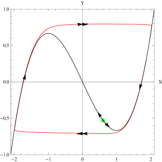
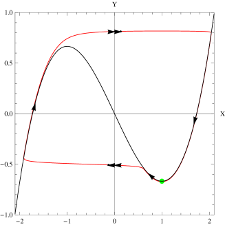
(a) $\mu<0.99874$		(b) $\mu=0.99874045$
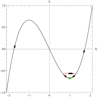
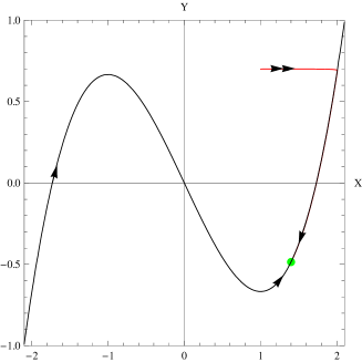
(c) $\mu=0.998740451$		(d) $\mu>1$

Figure 1. Transition from relaxation oscillation to canard explosion.

4. Flow Curvature Method

Recently, a new approach called Flow Curvature Method and based on the use of Differential Geometry properties of curvatures has been developed, see [16, 17]. According to this method, the highest curvature of the flow, i.e. the $(n-1)^{th}$ curvature of trajectory curve integral of $n$–dimensional dynamical system defines a manifold associated with this system and called flow curvature manifold. In the case of $n$–dimensional singularly perturbed dynamical system (1) for which with $\vec{x}\in\mathbb{R}^{1}$, $\vec{z}\in\mathbb{R}^{n-1}$, i.e. $(m,p)=(1,n-1)$ we have the following result.

Proposition 3.

The location of the points where the $(n-1)^{th}$ curvature of the flow, i.e. the curvature of the trajectory curve $\vec{X}$, integral of any $n$–dimensional singularly perturbed dynamical system vanishes, represents its $(n-1)$–dimensional slow manifold $M_{\varepsilon}$ the equation of which reads

(15) $$\phi({\vec{X},\varepsilon})=\dot{\vec{X}}\cdot({\ddot{\vec{X}}\wedge\dddot{\vec{X}}\wedge\ldots\wedge\mathop{\vec{X}}\limits^{\left(n\right)}})=\det({\dot{\vec{X}},\ddot{\vec{X}},\dddot{\vec{X}},\ldots,\mathop{\vec{X}}\limits^{\left(n\right)}})=0$$

where $\mathop{\vec{X}}\limits^{\left(n\right)}$ represents the time derivatives up to order $n$ of $\vec{X}=(\vec{x},\vec{z})^{t}$.

Proof.

For proof of this proposition see [17, p. 185 and next] and below. ∎

Remark 4.

First, let’s notice that with the Flow Curvature Method the slow manifold is defined by an implicit equation. Secondly, in the most general case of $n$–dimensional singularly perturbed dynamical system (1) for which $\vec{x}\in\mathbb{R}^{m}$, $\vec{z}\in\mathbb{R}^{p}$ the Proposition 3 still holds. In dimension three, the example of a Neuronal Bursting Model (NBM) for which $(m,p)=(2,1)$ has already been studied by Ginoux et al. [15]. In this particular case, one of the hypotheses of the Tihonov’s theorem is not checked since the fast dynamics of the singular approximation has a periodic solution. Nevertheless, it has been established by Ginoux et al. [15] that the slow manifold can all the same be obtained while using the Flow Curvature Method. According to this method, the slow invariant manifold of a three-dimensional singularly perturbed dynamical system for which $(m,p)=(1,2)$ is given by the $2^{nd}$ curvature of the flow, i.e. the torsion. In the case of a Neuronal Bursting Model for which $(m,p)=(2,1)$ it has been stated by Ginoux et al. [15] that the slow manifold is then given by the $1^{st}$ curvature of the flow, i.e. the curvature. In such a case, the flow curvature manifold is defined by the location of the points where the three-dimensional pseudovector $\dot{\vec{X}}\wedge\ddot{\vec{X}}$ vanishes. This condition leads to a nonlinear system of three equations two of which being linearly independent. These two equations define a curve corresponding to the slow invariant manifold. Thus, one can deduce that for a three-dimensional singularly perturbed dynamical system for which $(m,p)$ the slow manifold is given by the $p^{th}$ curvature of the flow.

4.1. Invariance

According to Schlomiuk [27] and Llibre et al. [24] the concept of invariant manifold has been originally introduced by Gaston Darboux [7, p. 71] in a memoir entitled: Sur les équations différentielles algébriques du premier ordre et du premier degré and can be stated as follows.

Proposition 5.

The manifold defined by $\phi(\vec{X},\varepsilon)=0$ where $\phi$ is a $C^{1}$ in an open set U, is invariant with respect to the flow of (1) if there exists a $C^{1}$ function denoted by $\kappa(\vec{X},\varepsilon)$ and called cofactor which satisfies

(16) $$L_{\overrightarrow{V}}\phi(\vec{X},\varepsilon)=\kappa(\vec{X},\varepsilon)\phi(\vec{X},\varepsilon),$$

for all $\vec{X}\in U$, and with the Lie derivative operator defined as

$$L_{\overrightarrow{V}}\phi=\overrightarrow{V}\cdot\overrightarrow{\nabla}\phi=\sum\limits_{i=1}^{n}{\frac{\partial\phi}{\partial x_{i}}\dot{x}_{i}}=\frac{d\phi}{dt}.$$

Proof.

According to Fenichel’s Persistence Theorem (see Th. 2) the slow invariant manifold $M_{\varepsilon}$ may be written as an explicit function $\vec{x}=\vec{F}\left({\vec{z},\varepsilon}\right)$, the invariance of which implies that $\vec{F}\left({\vec{z},\varepsilon}\right)$ satisfies

(17) $$\varepsilon D_{\vec{z}}\vec{F}\left({\vec{z},\varepsilon}\right)\vec{g}\left({\vec{F}\left({\vec{z},\varepsilon}\right),\vec{z},\varepsilon}\right)=\vec{f}\left({\vec{F}\left({\vec{z},\varepsilon}\right),\vec{z},\varepsilon}\right)$$

We write the slow manifold $M_{\varepsilon}$ as an implicit function by posing

(18) $$\phi(\vec{x},\vec{z},\varepsilon)=\vec{x}-\vec{F}\left(\vec{z},\varepsilon\right)=\phi(\vec{X},\varepsilon).$$

According to Darboux invariance theorem $M_{\varepsilon}$ is invariant if its Lie derivative reads

(19) $$L_{\vec{V}}\phi(\vec{X},\varepsilon)=\kappa(\vec{X},\varepsilon)\phi(\vec{X},\varepsilon).$$

Plugging Eq. (18) into the Lie derivative (19) leads to

$$L_{\vec{V}}\phi(\vec{X},\varepsilon)=\dot{\vec{x}}-D_{\vec{z}}\vec{F}(\vec{z},\varepsilon)\dot{\vec{z}}=\kappa(\vec{X},\varepsilon)\phi(\vec{X},\varepsilon),$$

which may be written according to Eq. (2) as

$$L_{\vec{V}}\phi(\vec{X},\varepsilon)=\frac{1}{\varepsilon}(\vec{f}(\vec{X},\varepsilon)-\varepsilon D_{\vec{z}}\vec{F}({\vec{z},\varepsilon})\vec{g}(\vec{X},\varepsilon))=\kappa(\vec{X},\varepsilon)\phi(\vec{X},\varepsilon).$$

Evaluating this Lie derivative in the location of the points where $\phi(\vec{X},\varepsilon)=0$, i.e. $\vec{x}=\vec{F}(\vec{z},\varepsilon)$ leads to

$$L_{\vec{V}}\phi(\vec{F}\left(\vec{z},\varepsilon\right),\vec{z},\varepsilon)=\frac{1}{\varepsilon}\left(\vec{f}(\vec{F}\left(\vec{z},\varepsilon\right),\vec{z},\varepsilon)-\varepsilon D_{\vec{z}}\vec{F}\left({\vec{z},\varepsilon}\right)\vec{g}(\vec{F}\left(\vec{z},\varepsilon\right),\vec{z},\varepsilon)\right)=0,$$

which is exactly identical to Eq. (18) used by Fenichel. ∎

Remark 6.

This last equation for the invariance of the manifold $M_{\varepsilon}$ may be written in a simpler way which implies that $\phi({\vec{x},\vec{z},\varepsilon})$ satisfies

(20) $$\dfrac{d}{dt}\left[\phi({\vec{x},\vec{z},\varepsilon})\right]=0,$$

on the solutions of the differential system.

4.2. Slow invariant manifold

We consider again the following two-dimensional singularly perturbed dynamical system

$$\varepsilon\dot{x} =f(x,y),$$

$$\dot{y} =g(x,y),$$

and we suppose that due to the nature of the problem perturbation expansion reads

$$y=F(x,\varepsilon)=F_{0}(x)+\varepsilon F_{1}(x)+\varepsilon^{2}F_{2}(x)+O\left(\varepsilon^{3}\right).$$

According to the Flow Curvature Method each function $\vec{F_{i}}(\vec{z})$ of this perturbation expansion may be found again starting from the slow manifold implicit equation (16) as stated in the next result.

Proposition 7.

The functions $F_{i}(x)$ of the slow invariant manifold associated with a two-dimensional singularly perturbed dynamical system are given by the following expressions

(21) $$\begin{array}[]{*{20}c}F^{\prime}_{n}(x)=\mathop{\lim}\limits_{\varepsilon\to 0}\left[{\dfrac{1}{n!}\dfrac{\partial^{n}a_{10}}{\partial\varepsilon^{n}}}\right]\mbox{ with }n\geq 0,\vspace{4pt}\\ F_{n}(x)=\mathop{\lim}\limits_{\varepsilon\to 0}\left[{\dfrac{1}{n!}\dfrac{\partial^{n-1}a_{01}}{\partial\varepsilon^{n-1}}}\right]\mbox{ with }n\geq 1,\end{array}$$

where

$$a_{10}=-\left.{\dfrac{\dfrac{\partial\phi_{i}}{\partial x}}{\dfrac{\partial\phi_{i}}{\partial y}}}\right|_{y=F\left({x,\varepsilon}\right)}\quad\mbox{and}\qquad a_{01}=-\left.{\dfrac{\dfrac{\partial\phi_{i}}{\partial\varepsilon}}{\dfrac{\partial\phi_{i}}{\partial y}}}\right|_{y=F\left({x,\varepsilon}\right)},$$

and

$$\phi_{i}(x,y,\varepsilon)=\frac{d^{i-1}}{dt^{i-1}}[\phi_{1}(x,y,\varepsilon)]\quad\mbox{with}\quad\mbox{i = 1, 2, ..., n},$$

where $\phi_{i}(x,y,\varepsilon)$ corresponds to the $i^{th}$ order approximation in $\varepsilon$.

Proof.

We have that

$$\phi({\vec{X},\varepsilon})=\left\|{\dot{\vec{X}}\wedge\ddot{\vec{X}}}\right\|=\det({\dot{\vec{X}},\ddot{\vec{X}}})=0\quad\Leftrightarrow\quad\phi\left({x,y,\varepsilon}\right)=0.$$

Since, for a two-dimensional singularly perturbed dynamical systems this slow manifold equation is defined by the second order tensor of curvature, i.e. by a determinant involving the first and second time derivatives of the vector field $\vec{X}$, it corresponds to the first order approximation in $\varepsilon$ of the slow manifold obtained with the Geometric Singular Perturbation Method. So, we denote it by

$$\phi_{1}({\vec{X},\varepsilon})=\left\|{\dot{\vec{X}}\wedge\ddot{\vec{X}}}\right\|=\det({\dot{\vec{X}},\ddot{\vec{X}}})=0.$$

A third order tensor of curvature can be easily given by the time derivative of $\phi_{1}({\vec{X},\varepsilon})$. We denote it by

$$\phi_{2}({\vec{X},\varepsilon})=\dot{\phi}_{1}({\vec{X},\varepsilon})=\det({\dot{\vec{X}},\dddot{\vec{X}}})=0.$$

Thus, $\phi_{2}({\vec{X},\varepsilon})$ corresponds to the second order approximation in $\varepsilon$. Using the same process, we consider the slow manifold $\phi_{i}({\vec{X},\varepsilon})$ which corresponds to the $i^{th}$ order approximation in $\varepsilon$.

Writing the total differential of the slow manifold we obtain

(22) $$d\phi_{i}\left({x,y,\varepsilon}\right)=\dfrac{\partial\phi_{i}}{\partial x}dx+\dfrac{\partial\phi_{i}}{\partial y}dy+\dfrac{\partial\phi_{i}}{\partial\varepsilon}d\varepsilon=0.$$

Replacing in Eq. (23) $dy$ by its total differential $dy=\dfrac{\partial F}{\partial x}dx+\dfrac{\partial F}{\partial\varepsilon}d\varepsilon$ yields

(23) $$d\phi_{i}(x,y,\varepsilon)=\left(\dfrac{\partial\phi_{i}}{\partial x}+\dfrac{\partial\phi_{i}}{\partial y}\dfrac{\partial F}{\partial x}\right)dx+\left(\dfrac{\partial\phi_{i}}{\partial\varepsilon}+\dfrac{\partial\phi_{i}}{\partial y}\dfrac{\partial F}{\partial\varepsilon}\right)d\varepsilon.$$

According to Eq. (21) $\phi_{i}(x,y,\varepsilon)$ is invariant if and only if $d\phi_{i}(x,y,\varepsilon)=0$, i.e. if

(24) $$\dfrac{\partial\phi_{i}}{\partial x}+\dfrac{\partial\phi_{i}}{\partial y}\dfrac{\partial F}{\partial x}=0\quad\Leftrightarrow\quad\dfrac{\partial F}{\partial x}=-\dfrac{\dfrac{\partial\phi_{i}}{\partial x}}{\dfrac{\partial\phi_{i}}{\partial y}},$$

$$\dfrac{\partial\phi_{i}}{\partial\varepsilon}+\dfrac{\partial\phi_{i}}{\partial y}\dfrac{\partial F}{\partial\varepsilon}=0\quad\Leftrightarrow\quad\dfrac{\partial F}{\partial\varepsilon}=-\dfrac{\dfrac{\partial\phi_{i}}{\partial\varepsilon}}{\dfrac{\partial\phi_{i}}{\partial y}}.$$

By replacing $y=F\left(x,\varepsilon\right)$ by its expression in both parts of Eq. (25) and by setting

$$a_{10}=-\left.{\dfrac{\dfrac{\partial\phi_{i}}{\partial x}}{\dfrac{\partial\phi_{i}}{\partial y}}}\right|_{y=F\left({x,\varepsilon}\right)}\quad\mbox{and}\qquad a_{01}=-\left.{\dfrac{\dfrac{\partial\phi_{i}}{\partial\varepsilon}}{\dfrac{\partial\phi_{i}}{\partial y}}}\right|_{y=F\left({x,\varepsilon}\right)},$$

we have that

(25) $$\begin{array}[]{*{20}c}\dfrac{\partial F\left({x,\varepsilon}\right)}{\partial x}=F^{\prime}_{0}(x)+\mbox{ }\varepsilon F^{\prime}_{1}(x)+O\left({\varepsilon^{2}}\right)=a_{10},\vspace{4pt}\\ \dfrac{\partial F\left({x,\varepsilon}\right)}{\partial\varepsilon}=F_{1}(x)+2\varepsilon F_{2}(\varepsilon)+O\left({\varepsilon^{2}}\right)=a_{01}.\\ \end{array}$$

By using a recurrence reasoning it may be easily stated that the functions $F_{i}(x)$ of the slow invariant manifold associated with a two-dimensional singularly perturbed dynamical system are given by the expressions (21). ∎

4.3. Van der Pol’s “canards”

We consider again the Van der Pol system (12). All functions $F_{i}(x)$ of the perturbation expansion may be deduced from the slow manifold equation defined by (16). But, since the determination of $F_{3}(x)$, i.e. the computation $\mu_{2}$ requires a third order tensor of curvature we consider $\phi_{3}({\vec{X},\varepsilon})$ the second time derivative of $\phi_{1}({\vec{X},\varepsilon})$ which corresponds to the third order approximation in $\varepsilon$.

Thus, we find at

Order $\varepsilon^{0}$

$$F^{\prime}_{0}(x)=\mathop{\lim}\limits_{\varepsilon\to 0}\left[a_{10}\right]=-1+x^{2},$$

from which one deduces that

$$F_{0}(x)=\dfrac{x^{3}}{3}-x+C_{0},$$

where the constant $C_{0}$ may be chosen in such a way that the critical manifold can be found again ($C_{0}=0$).

Order $\varepsilon^{1}$

(26) $$F_{1}(x)=\mathop{\lim}\limits_{\varepsilon\to 0}\left[a_{01}\right]=\dfrac{\mu_{0}-x}{x^{2}-1}.$$

Thus, one find again exactly the same functions $F_{1}(x)$ as those given by Geometric Singular Perturbation Method (14) and of course the same value of the bifurcation parameter $\mu_{0}=1$.

Order $\varepsilon^{2}$

(27) $$F_{2}(x)=\dfrac{\mu_{1}+\dfrac{(x-\mu_{0})(x^{2}+1-2\mu_{0}x)}{(x^{2}-1)^{3}}}{x^{2}-1}.$$

Taking into account that $\mu_{0}=1$ we find again exactly the same functions $F_{2}(x)$ as those given by Geometric Singular Perturbation Method (15) and of course the same value of the bifurcation parameter $\mu_{1}=-1/8$.

Order $\varepsilon^{3}$

A simple and direct computation leads to $\mu_{2}=-\dfrac{3}{32}$. Thus, the bifurcation parameter value leading to canard solutions reads

$$\mu=1-\dfrac{1}{8}\varepsilon-\dfrac{3}{32}\varepsilon^{2}+O\left({\varepsilon^{3}}\right).$$

Then, for $\varepsilon=0.01$ one finds again the value obtained by Benoît et al. [2, p.99] and Diener [8]

$$\mu=0.99874...$$

A program made with Mathematica and available at: http://ginoux.univ-tln.fr enables to compute all order of approximations in $\varepsilon$ of any two-dimensional singularly perturbed systems.

5. Conclusion

Thus, the bifurcation parameter value leading to a canard explosion in dimension two obtained by the so-called Geometric Singular Perturbation Method has been found again with the Flow Curvature Method. This result could be also extended to three-dimensional singularly perturbed dynamical systems such as the 3D-autocatalator in which canard phenomenon occurs.

References

- [1] A.A. Andronov & S.E. Chaikin, Theory of Oscillators, I. Moscow, 1937; English transl., Princeton Univ. Press, Princeton, N.J., 1949.
- [2] E. Benoît, J.L. Callot, F. Diener & M. Diener, Collectanea Mathematica 31-32 (1-3) (1981) 37-119.
- [3] M. Brns & K. Bar-Eli, J. Phys. Chem., Vol. 95 (22) (1991) 8706-8713.
- [4] M. Brns & K. Bar-Eli, Proc. R. Soc. Lond. A 445 (1994) 305-322.
- [5] M. Canalis-Durand, F. Diener and M. Gaetano, Calcul des valeurs à canard à l’aide de Macsyma, in Mathématiques finitaires et Analyse Non Standard, Ed. M. Diener and G. Wallet, Publications mathématiques de l’Université Paris 7 (1985), pp ”153–167”.
- [6] J.D. Cole, Perturbation Methods in Applied Mathematics, Blaisdell, Waltham, MA, 1968.
- [7] G. Darboux, Bull. Sci. Math. 2(2) (1878) 60-96, 123-143 & 151-200.
- [8] M. Diener, The Mathematical Intelligencer 6 (1984) 38-49.
- [9] F. Dumortier & R. Roussarie, Canard cycles and center manifolds, Memoires of the AMS, 557, 1996.
- [10] W. Eckhaus, Relaxation oscillations including a standard chase on French ducks; in Asymptotic Analysis II, Springer Lecture Notes Math. 985 (1983) 449-494.
- [11] N. Fenichel, Ind. Univ. Math. J. 21 (1971) 193-225.
- [12] N. Fenichel, Ind. Univ. Math. J. 23 (1974) 1109-1137.
- [13] N. Fenichel, Ind. Univ. Math. J. 26 (1977) 81-93.
- [14] N. Fenichel, J. Diff. Eq. 31 (1979) 53-98.
- [15] J.M. Ginoux & B. Rossetto, Slow manifold of a neuronal bursting model, in Emergent Properties in Natural and Articial Dynamical Systems (eds M.A. Aziz-Alaoui & C. Bertelle), Springer-Verlag, 2006, pp. 119-128.
- [16] J.M. Ginoux, B. Rossetto & L.O. Chua, Int. J. Bif. & Chaos 11(18) (2008) 3409-3430.
- [17] J.M. Ginoux, Differential geometry applied to dynamical systems, World Scientific Series on Nonlinear Science, Series A 66 (World Scientific, Singapore), 2009.
-
[18]
R. Gilmore, J.M. Ginoux, T. Jones, C Letellier & U. S. Freitas,
J. Phys. A: Math. Theor. 43 (2010) 255101 (13pp). - [19] M. W. Hirsch, C.C. Pugh & M. Shub, Invariant Manifolds, Springer-Verlag, New York, 1977.
- [20] C.K.R.T. Jones, Geometric Singular Pertubation Theory, in Dynamical Systems, Montecatini Terme, L. Arnold, Lecture Notes in Mathematics, vol. 1609, Springer-Verlag, 1994, pp. 44-118.
- [21] T. Kaper, An Introduction to Geometric Methods and Dynamical Systems Theory for Singular Perturbation Problems, in Analyzing multiscale phenomena using singular perturbation methods, (Baltimore, MD, 1998), pages 85-131. Amer. Math. Soc., Providence, RI, 1999.
- [22] M. Krupa & P. Szmolyan, J. Diff. Eq. 174 (2001) 312-368.
- [23] N. Levinson, Ann. Math. 50 (1949) 127-153.
- [24] J. Llibre & J.C. Medrado, J. Phys. A: Math. Theor. 40 (2007) 8385-8391.
- [25] R.E. O’Malley, Introduction to Singular Perturbations, Academic Press, New York, 1974.
- [26] R.E. O’Malley, Singular Perturbations Methods for Ordinary Differential Equations, Springer-Verlag, New York, 1991.
- [27] D. Schlomiuk, Expositiones Mathematicae 11 (1993) 433-454.
- [28] Szmolyan, M. Wechselberger, J. Diff. Eq. 177 (2001) 419-453.
- [29] F. Takens, Constrained equations; A study of implicit differential equations and their discontinuous solutions, in Lecture Notes in Mathematics volume 525 (1976), Springer Verlag.
- [30] A.N. Tikhonov, Mat. Sbornik N.S., 31 (1948) 575-586.
- [31] B. Van der Pol, Phil. Mag., 7(2) (1926) 978-992.
- [32] W.R. Wasow, Asymptotic Expansions for Ordinary Differential Equations, Wiley-Interscience, New York, 1965.