Conformal invariance predictions for the
three-dimensional self-avoiding walk

Abstract

If the three dimensional self-avoiding walk (SAW) is conformally invariant, then one can compute the hitting densities for the SAW in a half-space and in a sphere [14]. The ensembles of SAW’s used to define these hitting densities involve walks of arbitrary lengths, and so these ensembles cannot be directly studied by the pivot Monte Carlo algorithm for the SAW. We show that these mixed length ensembles should have the same scaling limit as certain weighted ensembles that only involve walks with a single length, thus providing a fast method for simulating these ensembles. Preliminary simulations which found good agreement between the predictions and Monte Carlo simulations for the SAW were reported in [14]. In this paper we present more accurate simulations testing the predictions and find even stronger support for the prediction that the SAW is conformally invariant in three dimensions.

1 Introduction

The scaling limit of the self-avoiding walk (SAW) is conjectured to be conformally invariant. In two dimensions this conjecture leads to a complete description of the scaling limit. If $D$ is a simply connected domain, the scaling limit of the SAW between two fixed boundary points is conjectured to be chordal Schramm-Lowener evolution (SLE) with parameter $\kappa=8/3$ [15]. (Between a fixed boundary point and a fixed interior point the scaling limit is conjectured to be radial SLE.) If one considers SAW’s in $D$ which start at a fixed interior point but are allowed to end anywhere on the boundary, then there are predictions for the distribution of the terminal point [15]. Monte Carlo tests of the SLE predictions for the two-dimensional SAW can be found in [5, 10, 11]. Tests of the predictions for the hitting density can be found in [12, 13] All these simulations found excellent agreement with the predictions, supporting the conjecture that the two-dimensional SAW is conformally invariant.

The success of using conformal invariance to study the two dimensional SAW is a result of the large group of conformal transformations in two dimensions. In three and higher dimensions this group consists only of compositions of Euclidean symmetries and inversions in spheres. It is not expected that invariance under this limited group completely determines the SAW in three dimensions, but one can still ask if the SAW is conformally invariant and if this invariance leads to any non-trivial predictions for the three-dimensional SAW. We restrict our attention to three dimensions since the scaling limit of the SAW has been proved to be Brownian motion in more than four dimensions [7, 8], and substantial progress toward proving this in four dimensions has been made [1].

In [14] we argued that the conformal covariance prediction of [15] for the hitting density in two dimensions holds in three dimensions as well. This led to a prediction of the hitting density for the SAW starting at an interior point of the half-space $z>0$ and the hitting density of the SAW starting at an interior point of a sphere. The conjectured conformal invariance also gives a prediction for the distribution of the first time the SAW in the full-space between two fixed points crosses the plane which bisects the line segment between those two points. These three predictions for the SAW were tested by Monte Carlo simulations of the SAW, and the results of those simulations were reported in [14]. We found good agreement between the simulations and the conformal invariance predictions, supporting the conjecture that the SAW is conformally invariant in three dimensions.

The ensembles of SAW’s in these predictions are not easily studied by the usual Monte Carlo algorithms for the SAW, in particular the pivot algorithm. The simulations presented in [14] relied on a representation of these ensembles in terms of the ensemble of SAW’s with a fixed number of steps and no constraint on the end point. In this paper we derive these representations. We also explain the lattice effects that persist in the scaling limit that must be taken into account.

In the next section we review the definition of the SAW and the predictions derived in [14]. In section three we derive the representations of the ensembles we wish to study in terms of the ensemble of SAW’s with a fixed number of steps. The lattice effects that persist in the scaling limit are studied in section four. Section five presents the results of the simulations, and the final section presents our conclusions.

2 Definitions and predictions

We review the definition of the self-avoiding walk. We introduce a lattice with spacing $\delta$, e.g., $\delta{\mathbb{Z}}^{d}$. Our simulations use the cubic lattice, but our predictions about the scaling limit should hold for any regular lattice in three dimensions. A self-avoiding walk is a nearest-neighbor walk on the lattice which does not visit any site in the lattice more than once. We will denote such a walk by $\omega(i)$ where $i=0,1,2,\cdots,N$ with $N$ being the number of steps in the walk. So $\omega$ satisfies $|\omega(i)-\omega(i-1)|=\delta$ for $i=1,2,\cdots,N$ and $\omega(i)\neq\omega(j)$ for $i\neq j$. In this paper we will always take the SAW to start at the origin, i.e., $\omega(0)=0$. There are a variety of ensembles that one can consider. One can consider the SAW on the full lattice, or one can only allow SAW’s that lie inside some prescribed domain. One can consider SAW’s which start and end at prescribed points, or one can consider SAW’s which start at a prescribed point but are allowed to end in some set, e.g., the boundary of a domain.

We start with the SAW in a bounded domain. Let $D$ be a bounded domain containing the origin or with the origin on its boundary. The ordinary random walk in $D$ started at the origin and stopped when it exits $D$ may be described as follows. We consider all finite nearest neighbor walks in $D$ which start at the origin and stay inside $D$ except for the last step of the walk which takes it outside $D$. Such a walk $\omega$ is given probability ${z}^{-|\omega|}$ where ${z}$ is the coordination number of the lattice. We define the SAW in $D$ starting at the origin in an analogous fashion. In place of the coordination number we use the connective constant $\mu$. It is given by $\mu=\lim_{N\rightarrow\infty}c_{N}^{1/N}$ where $c_{N}$ denotes the number of SAW’s on the full lattice with $N$ steps that start at $0$. (The existence of this limit follows from the subadditivity of $\ln(c_{N})$ [16].) The SAW in $D$ is then defined by taking all SAW’s that start at the origin and stay inside $D$ except for the last bond which takes the walk outside of $D$. The probability of such a walk $\omega$ is defined to be proportional to $\mu^{-|\omega|}$. (The constant of proportionality is determined by the requirement that we get a probability measure.) Rather than allow the SAW to end at any site just outside the boundary, we could also fix both the starting point and an ending point just outside $D$ and consider the ensemble of SAW’s between these two points that stay inside $D$ except for the last step. When $D$ is unbounded, there are infinitely many SAW’s between the two points, and it is not clear whether the sum of the weight $\mu^{-|\omega|}$ is finite.

We would also like to consider the SAW in an unbounded domain when the terminal point is taken to be $\infty$. In this case we need to modify the definition. There are two possible definitions. For the first, we fix an integer $N$ and take all SAW’s which start at the prescribed starting point, stay inside $D$ and have exactly $N$ steps. We put the uniform probability measure on this finite set of walks. It is expected that as $N\rightarrow\infty$, this probability measure converges weakly to a probability measure supported on infinite SAW’s from the starting point to $\infty$. The other definition is to consider all finite length SAW’s starting at the prescribed starting point and staying in $D$. The weight of a walk $\omega$ is taken to be $c^{-|\omega|}$ with $c>\mu$. This inequality insures that the resulting measure is finite and so can be normalized to give a probability measure. We then expect that as $c\rightarrow\mu^{+}$ this probability measure converges weakly to a probability measure supported on infinite SAW’s from the starting point to $\infty$. It is expected that the two definitions produce the same probability measure.

For all these ensembles the scaling limit should be obtained by letting $\delta\rightarrow 0$. It is expected that the probability measures converge weakly in this limit to probability measures supported on simple curves, but this has not been proven.

We review the definitions of several critical exponents that we will use. The average distance that an $N$ step SAW travels is described by the exponent $\nu$.

$$E_{N}[||\omega(N)||^{2}]\sim N^{2\nu}$$

where $E_{N}$ is expectation with respect to the uniform probability measure on SAW’s with $N$ steps starting at the origin. The exponents $\gamma$ and $\rho$ characterize the asymptotic behavior of the number of SAW’s. The number of SAW’s with $N$ steps starting at the origin grows as $\mu^{N}N^{\gamma-1}$. If you only allow SAW’s that stay in a half-space, e.g., $\{(x,y,z):z>0\}$, or in two dimensions in a half-plane, then it grows like $\mu^{N}N^{\gamma-1-\rho}$. So the probability that a SAW with $N$ steps in the full-space lies in the half-space goes like $N^{-\rho}$. The final exponent we need is the boundary scaling exponent $b$. The partition function of the SAW between two fixed boundary points of a domain goes as $\delta^{2b}$ as the lattice spacing $\delta$ goes to zero. The exponent $b$ also characterizes the probability that a two-dimensional SAW will pass through a small slit in a curve. If $\epsilon$ is the width of the slit, the probability goes as $\epsilon^{2b}$ as $\epsilon$ goes to zero. This holds in three dimensions as well if $\epsilon$ is the linear size of a small hole in a surface.

In two dimensions there are predictions for the values of these exponents, none of which have been proved. (In fact the existence of these exponents is not even established rigorously in two and three dimensions.) The predictions are $\nu=3/4$ [6], $\gamma=43/32$ [17], $\rho=25/64$ [2] and $b=\eta_{\parallel}/2=5/8$ [2]. In three dimensions there are numerical estimates for these exponents but no exact predictions. In three dimensions Clisby [4] finds $\nu=0.587597(7)$ Schram, Barkema and Bisseling [18], find $\gamma=1.15698(34)$. Grassberger [9] finds $\gamma_{1}=0.6786\pm 0.0012$ where $\gamma_{1}=\gamma-\rho$.

These exponents are related by a standard scaling relation:

$$b={2\rho-\gamma\over 2\nu}+{d\over 2}$$ (1)

A heuristic derivation of this relation for the SAW can be found in [15]. They gave the derivation in two dimensions, but the derivation works in any number of dimensions.

For an ensemble in which the terminal point is allowed to be anywhere along the boundary we will refer to the distribution of this random terminal point as a hitting distribution. For the ordinary random walk the scaling limit of this distribution is harmonic measure. For the SAW there is another distribution on the boundary that can be defined. One can consider the SAW in the full-plane or space from $0$ to $\infty$ and look at the first exit from $D$. We emphasize that this distribution is not expected to be the same as the distribution we refer to as the hitting distribution. There are no predictions for this distribution defined using the SAW in the full-plane or space, and we will not consider it in this paper.

Lawler, Schramm, Werner gave a prediction for the hitting density of a SAW in two dimensions [15]. Let $D$ be a simply connected domain containing the origin and $f$ a conformal map such that $f(0)=0$. We denote the hitting density with respect to arc length by $\sigma_{D}(z)$ where $z\in\partial D$. Their prediction is that

$$\sigma_{D}(z)\propto\sigma_{f(D)}(f(z))\,|f^{\prime}(z)|^{b}$$ (2)

In particular, by taking $f$ to be a conformal map that sends $D$ to the unit disc, we see that $\sigma_{D}(z)$ is proportional to the density for harmonic measure on $\partial D$ raised to the $b$ power. Depending on just how one defines the ensemble of SAW’s that end on the boundary of $D$, there is a correction factor that must be included in the above prediction [12]. It arises from lattice effects that, somewhat surprisingly, persist in the scaling limit. This is discussed further in section 4.

A heuristic derivation of (2) can be found in [14]. The same argument holds in three dimensions with the caveat that the group of conformal transformations in three dimensions is quite limited. It is generated by translations, rotations, dilations and inversions in spheres. We will use the conformal transformation

$${f}(x,y,z)={2(x,y,1-z)\over x^{2}+y^{2}+(1-z)^{2}}$$

It maps the point at $\infty$ to the origin, maps the origin to the point $(0,0,2)$ and maps the unit sphere centered at the origin to the plane $z=1$. Note that this is the plane that bisects the line segment between the two endpoints, so we will often refer to it as the bisecting plane.

The first prediction we test is the hitting density for a SAW in the half-space $z<1$, starting at the origin and ending on the plane $z=1$. To derive the distribution of the endpoint on the plane we consider a SAW in the unit sphere centered at the origin which starts at the origin and ends on the surface of the sphere. The scaling limit of the hitting density should be uniform on the sphere. Under the conformal map (2) we have the SAW in the half-space $z<1$ starting at the origin. So if we let $(x,y,1)$ be the coordinates of a point on the plane $z=1$, then the density with respect to Lebesgue measure on the plane is

$$\sigma(x,y)\propto[x^{2}+y^{2}+1]^{-b}$$ (3)

The constant of proportionality is simply determined by the requirement that this is a probability density. (Details of this derivation can be found in [14].) Given the symmetry of the hitting density on the plane under rotations about the z-axis, we will just study the random variable $R=\sqrt{x^{2}+y^{2}}$. Its density is proportional to $r[r^{2}+1]^{-b}$, and so the cumulative distribution function (CDF) of $R$ is $P(R\leq r)=1-(r^{2}+1)^{1-b}$. The range of $R$ is unbounded, so it will be more convenient to display the simulation results using the angle $\Theta$ given by $\tan\Theta=R$. Its CDF is

$$P(\Theta\leq\theta)=1-(\cos\theta)^{2(b-1)}$$ (4)

The second prediction we test is the hitting density for a SAW in a sphere when the starting point is not the origin. Without loss of generality we can consider the unit sphere centered at the origin and take the starting point to be $(0,0,a)$ with $-1<a<1$. We parametrize the sphere with spherical coordinates, and let $\rho_{a}(\theta,\phi)$ be the hitting density with respect to Lebesgue measure on the sphere. Now we use the same conformal map (2) as before. It still takes the unit sphere to the plane $z=1$, and takes the starting point of the SAW at $(0,0,a)$ to $(0,0,2/(1-a))$. Using the results for the hitting density in a half-space we find

$$\rho_{a}(\theta,\phi)\propto\left[1+a^{2}-2a\cos(\theta)\right]^{-b}$$ (5)

(Details of this derivation can be found in [14].) If we only consider the angle $\Theta$, the density is

$$\rho_{a}(\theta)\propto\left[1+a^{2}-2a\cos(\theta)\right]^{-b}\,\sin(\theta)$$

Note that this can be explicitly integrated to give the CDF:

$$P(\Theta\leq\theta)={(1-a)^{2(1-b)}-(1+a^{2}-2a\cos(\theta))^{1-b}\over(1-a)^{2(1-b)}-(1+a)^{2(1-b)}}$$ (6)

The third prediction we test is for the SAW in the full space starting at the origin and ending at a fixed point which we take to be $(0,0,2)$. The prediction is for the distribution of the point where the walk first hits the plane $z=1$. To derive this distribution we consider the scaling limit of the SAW in the full-space from the origin to $\infty$. Look at the first time it hits the unit sphere. This point will be uniformly distributed over the sphere. The conformal map (2) transforms this into the SAW in the full-space from $(0,0,0)$ to $(0,0,2)$ and we are looking at the first hit of the plane $z=1$. So its distribution will just be the image of the uniform measure on the sphere under ${f}$. This is given by

$$\sigma_{first}(x,y)=\frac{1}{\pi}[x^{2}+y^{2}+1]^{-2}$$

Let $R=\sqrt{x^{2}+y^{2}}$, so $R$ is the distance from this first hit of the plane to the center of the plane. Then the density of $R$ is proportional to $[r^{2}+1]^{-2}\,r\,dr$. So $P(R\leq r)=\frac{r^{2}}{r^{2}+1}$. Again, we find it convenient to display our simulation results using the angle $\Theta$ given by $\tan\Theta=R$. Its CDF is

$$P(\Theta\leq\theta)=\sin^{2}\theta$$ (7)

3 Equivalence of ensembles

The most efficient algorithm for simulating the SAW is the pivot algorithm [16]. Clisby’s recent implementation of this algorithm has dramatically improved its efficiency [3]. The pivot algorithm simulates SAW ensembles with a fixed number of steps in the walk. The starting point of the walk is fixed, but the terminal point of the walk is not. In all of the ensembles we wish to study the number of steps is not fixed, and the terminal point of the walk is either fixed or constrained to lie on some boundary. So we cannot directly test the predictions of conformal invariance from the previous section with the pivot algorithm. Instead we will use the pivot algorithm to study ensembles that we believe to have the same scaling limit as the ensemble we considered in the previous section, but which are amenable to simulation by the pivot algorithm. The idea behind these ensembles was introduced in [13]. Although our focus is on three dimensions, the arguments in this section hold in any number of dimensions.

There are three SAW ensembles used in the paper. The “half-space ensemble” consists of all finite length SAW’s that start at the origin, and then stay in the half-space $z<1$ until they end somewhere on the plane $z=1$. The “spherical ensemble” consists of all finite length SAW’s that start at the origin and then stay inside the sphere of radius $1$ centered at $(0,0,-a)$ until they end somewhere on the surface of this sphere. The “point to point ensemble” consists of all finite length SAW’s in the full-space that start at the origin and end at a fixed point $q$. Note that all three of these ensembles share two features: there is no constraint on the number of steps in the walk, but there is a constraint on where the walk ends.

The pivot algorithm simulates the SAW ensemble which contains all SAW’s starting at the origin with a fixed number $N$ of steps and no constraint on where they end. We refer to this as the “fixed-length ensemble”, and denote expectations with respect to the uniform probability measure on these walks by $E_{N}$. The pivot algorithm can also be used to simulate the ensemble of SAW’s with $N$ steps which start at the origin and then stay in the half-space $z>0$. We refer to this as the “half-space fixed-length ensemble”, and denote expectations with respect to the uniform probability measure on it by $E_{N}^{+}$. In this section we show how to express the three ensembles used in this paper in terms of the fixed-length ensembles. In all three cases the general strategy is the same. We define a “super-ensemble” in which the number of steps in the SAW is not fixed and there are no constraints on where the SAW ends. We add a constraint to the super-ensemble that says that it is possible to transform the walk into a walk which appears in the desired ensemble by a Euclidean transformation. We then decompose the sum in the super-ensemble in two different ways. One decomposition shows that its scaling limit is the same as the scaling limit of the desired ensemble. The other decomposition shows that its scaling limit can be expressed in terms of the $N\rightarrow\infty$ limit of the fixed-length ensemble.

3.1 Half-space ensemble

We first consider the half-space ensemble which consists of all SAW’s on a lattice with spacing $\delta$ that start at the origin and then stay in the half-space $\{(x,y,z):z<1\}$ until they end on the boundary of this half-space, i.e., the plane $z=1$. A walk $\omega$ is given weight $\mu^{-|\omega|}$. We denote expectations in this half-space ensemble with lattice spacing $\delta$ by $E^{half}_{\delta}$. We want to express this half-space ensemble in terms of the half-space fixed-length ensemble which consists of all SAW’s with $N$ steps in the half-space $z>0$ that start at the origin. All the walks are given equal probability in the half-space fixed-length ensemble. We denote expectations in the half-space fixed-length ensemble by $E^{+}_{N}$. Given a walk from the half-space fixed-length ensemble we can reflect it in the plane $z=0$, then translate it and dilate it to produce a walk between the origin and the plane $z=1$ which stays in the half-space $z<1$, i.e., a walk in the half-space ensemble. If $\omega$ is the walk from the half-space fixed-length ensemble, we let $\omega(|\omega|)=(x_{0},y_{0},z_{0})$ and then let

$$\phi_{\omega}(x,y,z)=({x-x_{0}\over z_{0}},{y-y_{0}\over z_{0}},{z_{0}-z\over z_{0}})$$

Then $\phi_{\omega}$ is the Euclidean transformation that takes the endpoint of $\omega$ to the origin and takes the origin to some point on the plane $z=1$. So by reversing its direction we can think of $\phi_{\omega}(\omega)$ as a walk in the half-space ensemble. Our conjectured relationship between the half-space ensemble and the half-space fixed-length ensemble is as follows.

Equivalence of ensembles for the half-space: Let $\psi(\gamma)$ be a random variable on the space of simple curves $\gamma$ in the half-space $z<1$ which start at the origin and end somewhere on the plane $z=1$. Then

$$\lim_{\delta\rightarrow 0}E_{\delta}^{half}(\psi)=\lim_{{N}\rightarrow\infty}\frac{E^{+}_{N}[z({\overline{\omega}})^{p}\psi(\phi_{\overline{\omega}}({\overline{\omega}}))]}{E^{+}_{N}[z({\overline{\omega}})^{p}]}$$ (8)

where $p=\frac{\rho-\gamma}{\nu}$. The function $z(\omega)$ is the $z$-coordinate of $\omega(N)$, the endpoint of the walk. In words, we can simulate SAW’s from the half-space ensemble of walks that start at the origin and stay in the half-space $z<1$ until they end on the plane $z=1$ as follows. We generate walks ${\overline{\omega}}$ from the fixed-length ensemble, apply a Euclidean transformation so that the reversal of ${\overline{\omega}}$ goes from the origin to the plane $z=1$ and weight the walk by $z({\overline{\omega}})^{p}$.

To derive this relationship we use the super-ensemble which consists of all finite SAW’s in the half-space $z>0$ that start at the origin. A walk $\omega$ is weighted by $\mu^{-|\omega|}$. To ensure that the sum of the weights is finite we introduce a cutoff. For a walk $\omega$ we let $z(\omega)$ be the $z$-coordinate of $\omega(|\omega|)$, the endpoint of the walk. Fix $0<z_{1}<z_{2}$. Our cutoff is the condition $z_{1}\leq z(\omega)\leq z_{2}$. Define

$${\cal Z}_{\delta}(\psi)=\sum_{\omega:0\rightarrow{\mathbb{H}}}\mu^{-|\omega|}1(z_{1}\leq z(\omega)\leq z_{2})\,\psi(\phi_{\omega}(\omega))$$ (9)

where ${\mathbb{H}}$ stands for the half-space $z>0$ and the notation $\omega:0\rightarrow{\mathbb{H}}$ means that the sum is over all finite SAW’s which start at the origin and then stay in the half-space ${\mathbb{H}}$.

We now decompose the sum in ${\cal Z}_{\delta}(\psi)$ in two different ways. The first decomposition is based on where the walk ends.

$${\cal Z}_{\delta}(\psi)=\sum_{z_{1}\leq z\leq z_{2}}\quad\sum_{\omega:0\rightarrow{\mathbb{H}},z(\omega)=z}\mu^{-|\omega|}\,\psi(\phi_{\omega}(\omega))$$ (10)

The sum over $z$ is over multiples of $\delta$ that are in the allowed range. Define

$$Z_{\delta,z}=\sum_{\omega:0\rightarrow{\mathbb{H}},z(\omega)=z}\mu^{-|\omega|}\,$$

Consider

$${1\over Z_{\delta,z}}\sum_{\omega:0\rightarrow{\mathbb{H}},z(\omega)=z}\mu^{-|\omega|}\,\psi(\phi_{\omega}(\omega))$$

Thanks to the constraint $z(\omega)=z$, the transformations $\phi_{\omega}$ in this sum all have the same dilation factor, namely $1/z$. So the walks $\phi_{\omega}(\omega)$ all live on a lattice with spacing $\delta/z$. They all start at the origin and stay in the half-space $z<1$ until they end on the plane $z=1$. So the above is exactly equal to the expectation of $\psi$ in the half-space ensemble with lattice spacing $\delta/z$, i.e., $E^{half}_{\delta/z}[\psi]$. For all $z$, as $\delta\rightarrow 0$, this has the same limit as $E^{half}_{\delta}[\psi]$. Noting that

$$\sum_{z_{1}\leq z\leq z_{2}}Z_{\delta,z}={\cal Z}_{\delta}(1)$$

we conclude that

$$\lim_{\delta\rightarrow 0}{{\cal Z}_{\delta}(\psi)\over{\cal Z}_{\delta}(1)}=\lim_{\delta\rightarrow 0}E^{half}_{\delta}[\psi]$$ (11)

For the second decomposition of ${\cal Z}_{\delta}(\psi)$, we decompose it based on the number of steps in $\omega$. Let $b_{n}$ be the number of SAW’s in the half-space starting at $0$ with $n$ steps. We rewrite ${\cal Z}_{\delta}(\psi)$ as

$${\cal Z}_{\delta}(\psi) = \sum_{{n}=1}^{\infty}\mu^{-n}b_{n}\,{1\over b_{n}}\sum_{\omega:0\rightarrow{\mathbb{H}},|\omega|={n}}\,1(z_{1}\leq z(\omega)\leq z_{2})\,\psi(\phi_{\omega}(\omega))$$

$$= \sum_{{n}=1}^{\infty}\mu^{-{n}}b_{n}\,E^{+}_{n}[1(z_{1}\leq z(\omega)\leq z_{2})\,\psi(\phi_{\omega}(\omega))]$$

Since $z(\omega)\geq z_{1}$, $\omega$ must have at least $z_{1}/\delta$ steps. So as the lattice spacing goes to zero, the first $n$ for which the summand is nonzero goes to infinity. Since $b_{n}$ is asymptotic to $\mu^{{n}}{n}^{\gamma-1-\rho}$, we replace $b_{n}\mu^{-{n}}$ by ${n}^{\gamma-1-\rho}$. So we have

$${\cal Z}_{\delta}(\psi)\approx\sum_{{n}=1}^{\infty}{n}^{\gamma-1-\rho}\,E^{+}_{n}[1(z_{1}\leq z(\omega)\leq z_{2})\,\psi(\phi_{\omega}(\omega))]$$

Since the sum on ${n}$ is only over large values, we can replace the expectations $E^{+}_{n}$ over $\omega$ with a single expectation $E^{+}_{N}$ over ${\overline{\omega}}$ where ${N}$ is large. We replace $\omega{n}^{-\nu}$ with ${\overline{\omega}}{N}^{-\nu}$. So $z(\omega)$ becomes $z({n}^{\nu}{N}^{-\nu}{\overline{\omega}})={n}^{\nu}{N}^{-\nu}z({\overline{\omega}})$. And we replace $\psi(\phi_{\omega}(\omega))$ by $\psi(\phi_{\overline{\omega}}({\overline{\omega}}))$. We now have

$${\cal Z}_{\delta}(\psi)\approx\sum_{{n}=1}^{\infty}{n}^{\gamma-1-\rho}\,E^{+}_{N}[\,1(z_{1}\leq{n}^{\nu}{N}^{-\nu}z({\overline{\omega}})\leq z_{2})\,\psi(\phi_{\overline{\omega}}({\overline{\omega}}))]$$

The ${n}$ dependent part of the preceding sum is

$$\sum_{{n}=1}^{\infty}{n}^{\gamma-1-\rho}\,\,1(z_{1}\leq{n}^{\nu}{N}^{-\nu}z({\overline{\omega}})\leq z_{2})$$

If we multiply this by ${N}^{\rho-\gamma}$ it becomes a Riemann sum approximation to an integral, and we see that as ${N}\rightarrow\infty$,

$${N}^{\rho-\gamma}\sum_{{n}=1}^{\infty}{n}^{\gamma-1-\rho}\,\,1(z_{1}\leq{n}^{\nu}{N}^{-\nu}z({\overline{\omega}})\leq z_{2})=\frac{1}{{N}}\sum_{{n}=1}^{\infty}\left(\frac{{n}}{{N}}\right)^{\gamma-1-\rho}\,\,1(z_{1}\leq\left(\frac{{n}}{{N}}\right)^{\nu}z({\overline{\omega}})\leq z_{2})$$

$$\rightarrow\int_{0}^{\infty}x^{\gamma-1-\rho}\,1(z_{1}\leq x^{\nu}z({\overline{\omega}})\leq z_{2})\,dx=c\,[z({\overline{\omega}})]^{(\rho-\gamma)/\nu}$$

where the constant $c$ depends on $z_{1},z_{2},\rho,\gamma,\nu$. Thus

$$\lim_{\delta\rightarrow 0}\frac{{\cal Z}_{\delta}(\psi)}{{\cal Z}_{\delta}(1)}=\lim_{{N}\rightarrow\infty}\frac{E^{+}_{N}[z({\overline{\omega}})^{p}\psi(\phi_{\overline{\omega}}({\overline{\omega}}))]}{E^{+}_{N}[z({\overline{\omega}})^{p}]}$$ (12)

with $p=\frac{\rho-\gamma}{\nu}$. Combining eqs. (11) and (12) we obtain eq. (8).

3.2 Spherical ensemble

The second ensemble in the paper consists of all finite length SAW’s that start at $(0,0,a)$ and then stay inside the sphere of radius $1$ centered at the origin until they end somewhere on the surface of this sphere. (The parameter $a$ satisfies $-1<a<1$.) By a simple translation this becomes the ensemble of all walks that start at the origin and then stay inside the sphere of radius $1$ centered at $(0,0,-a)$ until they end somewhere on the surface of this sphere. A walk $\omega$ is given weight $\mu^{-|\omega|}$. We will refer to this ensemble of walks starting at the origin as the spherical ensemble, and denote expectations in this ensemble by $E^{sphere}_{\delta}$. We want to express this spherical ensemble in terms of the fixed-length ensemble which consists of all $N$ step walks in the full space which start at the origin. The walks are given equal probability in this ensemble, and we denote expectations by $E_{N}$. Given a walk $\omega$ from the fixed-length ensemble, there is a dilation factor $R(\omega)$ such that the dilated walk $\omega/R(\omega)$ will end on the surface of the sphere centered at $(0,0,-a)$ with radius $1$. In general this dilated walk will not stay inside the sphere, so we must condition on the event that it does. We let $1_{S}(\omega/R(\omega))$ denote the indicator function for this event. Our conjectured relationship between the spherical ensemble and the fixed-length ensemble is as follows.

Equivalence of ensembles for the sphere: Let $\psi(\gamma)$ be a random variable on the space of simple curves $\gamma$ from the origin to the boundary of the unit sphere centered at $(0,0,-a)$. Then

$$\lim_{\delta\rightarrow 0}E_{\delta}^{sphere}[\psi]=\lim_{{N}\rightarrow\infty}\frac{E_{N}[R({\overline{\omega}})^{p}\,1_{S}(\frac{{\overline{\omega}}}{R({\overline{\omega}})})\,W({\overline{\omega}})\psi(\frac{{\overline{\omega}}}{R({\overline{\omega}})})]}{E_{N}[R({\overline{\omega}})^{p}1_{S}(\frac{{\overline{\omega}}}{R({\overline{\omega}})})\,W({\overline{\omega}})]}$$ (13)

where $p=\frac{\rho-\gamma}{\nu}$. The function $W({\overline{\omega}})$ depends only on the endpoint of ${\overline{\omega}}$ and will be defined later. So we can simulate SAW’s from the spherical ensemble of walks that start at the origin and stay in the sphere of radius $1$ centered at $(0,0,-a)$ until they end on its boundary as follows. We generate walks ${\overline{\omega}}$ from the fixed-length ensemble. We rescale the walks so that they end on the given sphere and then condition on the event that the walk stays inside the sphere. These walks are then weighted by $R({\overline{\omega}})^{p}W({\overline{\omega}})$.

To derive this relationship we introduce the following super ensemble. We start with all finite SAW’s that start at the origin. A walk $\omega$ is weighted by $\mu^{-|\omega|}$. Fix $0<R_{1}<R_{2}$. Define

$${\cal Z}_{\delta}(\psi)=\sum_{\omega:0\rightarrow}\mu^{-|\omega|}1(R_{1}\leq R(\omega)\leq R_{2})\,1_{S}(\frac{\omega}{R(\omega)})\,W(\omega)\,\psi(\frac{\omega}{R(\omega)})$$ (14)

where the sum is over all finite SAW’s starting at the origin. $1_{S}(\frac{\omega}{R(\omega)})$ is the indicator function that the dilated walk stays in the sphere. We have introduced a cutoff by requiring $R(\omega)$ to lie between $R_{1}$ and $R_{2}$. Let $||\omega(|\omega|)||$ be the distance to the endpoint of $\omega$, and let $\theta$ be the angle between the $z$-axis and the line from the origin to the endpoint of $\omega$. Some calculation shows

$$R(\omega)=||\omega(|\omega|)||\frac{a\cos(\theta)+\sqrt{1-a^{2}\sin^{2}(\theta)}}{1-a^{2}}$$

We now decompose the sum in ${\cal Z}_{\delta}(\psi)$ in two different ways. The first decomposition is based on $R(\omega)$. We fix an $R$ and an infinitesimal $dR$ and consider the following “slice” of $Z_{\delta}(\psi)$.

$$\sum_{\omega:0\rightarrow}\mu^{-|\omega|}1(R\leq R(\omega)\leq R+dR)\,1_{S}(\frac{\omega}{R(\omega)})\,W(\omega)\,\psi(\frac{\omega}{R(\omega)})$$ (15)

The definition of $R(\omega)$ implies that $\omega$ ends on the surface of the sphere of radius $R(\omega)$ centered at $(0,0,-aR(\omega))$. So the sum above contains all walks that start at the origin and end in a thin shell about the surface of the sphere of radius $R$ centered at $(0,0,-aR)$. If the thickness of this shell were uniform and we did not include the factor of $W(\omega)$, then in the scaling limit the above sum with the appropriate normalization would converge to the expectation of $\psi$ in the spherical ensemble. However, the thickness of the shell is not uniform. We correct for this by taking $W(\omega)$ to be proportional to the reciprocal of the shell thickness. So $W(\omega)$ only depends on $\omega$ through its endpoint; in fact it is only a function of $\theta$. We can think of $Z_{\delta}(\psi)$ as a sum over many shells, and so we conclude that with this definition of $W(\omega)$,

$$\lim_{\delta\rightarrow 0}\frac{Z_{\delta}(\psi)}{Z_{\delta}(1)}=\lim_{\delta\rightarrow 0}E_{\delta}^{sphere}[\psi]$$ (16)

For the second decomposition of ${\cal Z}_{\delta}(\psi)$, we decompose it based on the number of steps in $\omega$. Let $c_{n}$ be the number of SAW’s starting at $0$ with ${n}$ steps. We rewrite ${\cal Z}_{\delta}(\psi)$ as

$${\cal Z}_{\delta}(\psi) = \sum_{{n}=1}^{\infty}\mu^{-{n}}c_{n}\,{1\over c_{n}}\sum_{\omega:0\rightarrow,|\omega|={n}}\,1(R_{1}\leq R(\omega)\leq R_{2})\,1_{S}(\frac{\omega}{R(\omega)})\,W(\omega)\,\psi(\frac{\omega}{R(\omega)})$$

$$= \sum_{{n}=1}^{\infty}\mu^{-{n}}c_{n}\,E_{n}[1(R_{1}\leq R(\omega)\leq R_{2})\,1_{S}(\frac{\omega}{R(\omega)})\,W(\omega)\psi(\frac{\omega}{R(\omega)})]$$

As the lattice spacing goes to zero, the first ${n}$ for which the summand in the sum on ${n}$ is nonzero goes to infinity. Since $c_{n}$ is asymptotic to $\mu^{{n}}{n}^{\gamma-1}$, we replace $\mu^{-{n}}c_{n}$ by ${n}^{\gamma-1}$. As in our previous derivation we replace the expectations $E_{n}$ by a single expectation $E_{N}$ by replacing ${n}^{-\nu}\omega$ with ${N}^{-\nu}{\overline{\omega}}$ where ${\overline{\omega}}$ comes from $E_{N}$. So $R(\omega)$ becomes $R({n}^{\nu}{N}^{-\nu}{\overline{\omega}})={n}^{\nu}{N}^{-\nu}R({\overline{\omega}})$. We can replace $\psi(\frac{\omega}{R(\omega)})$ by $\psi(\frac{{\overline{\omega}}}{R({\overline{\omega}})})$. The indicator function $1_{S}(\frac{\omega}{R(\omega)})$ is more subtle. The probability that an ${n}$-step SAW stays on one side of a half-plane is conjectured to go to zero as ${n}^{-\rho}$ as ${n}\rightarrow\infty$. So we expect that the probability that $1_{S}(\frac{\omega}{R(\omega)})=1$ also goes to zero as ${n}^{-\rho}$. So we approximate ${n}^{\rho}1_{S}(\frac{\omega}{R(\omega)})$ by ${N}^{\rho}1_{S}(\frac{{\overline{\omega}}}{R({\overline{\omega}})})$ i.e., we replace $1_{S}(\frac{\omega}{R(\omega)})$ by ${n}^{-\rho}{N}^{\rho}1_{S}(\frac{{\overline{\omega}}}{R({\overline{\omega}})})$. We now have

$${\cal Z}_{\delta}(\psi)\approx{N}^{\rho}\sum_{{n}=1}^{\infty}{n}^{\gamma-1-\rho}\,E_{N}[\,1(R_{1}\leq{n}^{\nu}{N}^{-\nu}R({\overline{\omega}})\leq R_{2})1_{S}(\frac{{\overline{\omega}}}{R({\overline{\omega}})})\,W({\overline{\omega}})\,\psi(\frac{{\overline{\omega}}}{R({\overline{\omega}})})]$$

The ${n}$ dependent part of this is

$$\sum_{{n}=1}^{\infty}{n}^{\gamma-1-\rho}\,\,1(R_{1}\leq{n}^{\nu}{N}^{-\nu}R({\overline{\omega}})\leq R_{2})$$

If we multiply this by ${N}^{\rho-\gamma}$ it becomes a Riemann sum approximation to an integral, and so as ${N}\rightarrow\infty$,

$${N}^{\rho-\gamma}\sum_{{n}=1}^{\infty}{n}^{\gamma-1-\rho}\,\,1(R_{1}\leq{n}^{\nu}{N}^{-\nu}R({\overline{\omega}})\leq R_{2})\rightarrow\int_{0}^{\infty}x^{\gamma-1-\rho}\,1(R_{1}\leq R({\overline{\omega}})x^{\nu}\leq R_{2})\,dx=cR({\overline{\omega}})^{(\rho-\gamma)/\nu}$$

Thus

$$\lim_{\delta\rightarrow 0}\frac{{\cal Z}_{\delta}(\psi)}{{\cal Z}_{\delta}(1)}=\lim_{{N}\rightarrow\infty}\frac{E_{N}[R({\overline{\omega}})^{p}\,1_{S}(\frac{{\overline{\omega}}}{R({\overline{\omega}})})\,W(\omega)\psi(\frac{{\overline{\omega}}}{R({\overline{\omega}})})]}{E_{N}[R({\overline{\omega}})^{p}1_{S}(\frac{{\overline{\omega}}}{R({\overline{\omega}})})\,W(\omega)]}$$ (17)

where $p=\frac{\rho-\gamma}{\nu}$. Combining eqs. (16) and (17) we obtain eq. (13).

3.3 Point to point ensemble

Finally, we consider the point to point ensemble of SAW’s. We take one point to be the origin and label the other point as $q$. The ensemble consists of all SAW’s on the lattice which start at $0$ and end at $q$. (We interpret ending at $q$ as meaning the walk ends at the nearest point in the lattice to $q$.) All finite length SAW’s between the points are allowed, and the probability of a walk $\omega$ is proportional to $\mu^{-|\omega|}$ where $|\omega|$ is the number of steps in the walk. We let $E_{\delta}^{0\rightarrow q}$ denote expectation with respect to this ensemble. As before $E_{N}$ denotes expectation in the fixed-length ensemble of walks in the full plane starting at the origin. Given a point $z$, in two dimensions there is a unique Euclidean symmetry that maps it to $q$ and fixes the origin. In three and higher dimensions, there are many Euclidean symmetries that do so. For each $z$ we pick one and denote it by $\phi_{z}$. Given a finite walk $\omega$ starting at $0$, $\phi_{\omega(|\omega|)}$ transforms $\omega$ into a walk from the origin to $q$. To simplify the notation we denote $\phi_{\omega(|\omega|)}$ just by $\phi_{\omega}$, but we emphasize that it only depends on the endpoint of $\omega$.

Equivalence of ensembles for the full space: Let $\psi(\gamma)$ be an observable on the space of simple curves $\gamma$ from $0$ to $q$. Then

$$\lim_{\delta\rightarrow 0}E_{\delta}^{0\rightarrow q}(\psi)=\lim_{{N}\rightarrow\infty}{E_{N}[||{\overline{\omega}}({N})||^{-\gamma/\nu}\psi(\phi_{\overline{\omega}}({\overline{\omega}}))]\over E_{N}[||{\overline{\omega}}({N})||^{-\gamma/\nu}]}$$ (18)

In words, we can simulate SAW’s from the ensemble of walks between $0$ and $q$ by generating walks ${\overline{\omega}}$ from the fixed-length ensemble, applying a Euclidean transformation so that the walk goes between $0$ and $q$ and weighting the walk by $||{\overline{\omega}}({N})||^{-\gamma/\nu}$.

To derive this relationship we use the super-ensemble consisting of all finite length SAW’s which start at the origin. The total mass of this ensemble is infinite, so we introduce a cutoff. Fix $0<r_{1}<r_{2}$. The cutoff is that $r_{1}\leq||\omega(|\omega|)||\leq r_{2}$. We define

$${\cal Z}_{\delta}(\psi)=\sum_{\omega:0\rightarrow}\mu^{-|\omega|}\,1(r_{1}\leq||\omega(|\omega|)||\leq r_{2})\,\psi(\phi_{\omega}(\omega))$$

where the sum is over all finite walks starting at $0$ on a lattice with spacing $\delta$. $\omega(|\omega|)$ is the endpoint of the walk, and $||\omega(|\omega|)||$ denotes the usual Euclidean distance of this point from the origin.

First we decompose the sum over walks in ${\cal Z}_{\delta}(\psi)$ based on where the walk ends:

$${\cal Z}_{\delta}(\psi)=\sum_{z}\sum_{\omega:0\rightarrow z}\mu^{-|\omega|}\,1(r_{1}\leq||z||\leq r_{2})\,\psi(\phi_{\omega}(\omega))$$

Define

$$Z_{\delta,z}=\sum_{\omega:0\rightarrow z}\mu^{-|\omega|}$$

So $Z_{\delta,z}$ is the partition function corresponding to $E_{\delta}^{0\rightarrow z}$. Then

$${\cal Z}_{\delta}(\psi) = \sum_{z:r_{1}\leq||z||\leq r_{2}}\,Z_{\delta,z}\,E_{\delta}^{0\rightarrow z}[\psi(\phi_{z}(\omega))]$$

We expect the scaling limit to have euclidean invariance, and so in the scaling limit
$E_{\delta}^{0\rightarrow z}[\psi(\phi_{z}(\omega))]$ and $E_{\delta}^{0\rightarrow q}[\psi(\omega)]$ should converge to the same limit for all $z$. The sum of $Z_{\delta,z}$ over $z$ satisfying $r_{1}\leq||z||\leq r_{2}$ is just ${\cal Z}_{\delta}(1)$. So

$$\lim_{\delta\rightarrow 0}\frac{{\cal Z}_{\delta}(\psi)}{{\cal Z}_{\delta}(1)}=\lim_{\delta\rightarrow 0}E_{\delta}^{0\rightarrow q}[\psi(\omega)]$$ (19)

Our second decomposition of ${\cal Z}_{\delta}(\psi)$ is based on the number of steps in the walk. Letting $c_{n}$ denote the number of SAW’s starting at the origin with ${n}$ steps, we have

$${\cal Z}_{\delta}(\psi) = \sum_{{n}=1}^{\infty}\mu^{-{n}}c_{n}\,{1\over c_{n}}\sum_{\omega:0\rightarrow,|\omega|={n}}\,1(r_{1}\leq||\omega({n})||\leq r_{2})\,\psi(\phi_{\omega}(\omega))$$

$$= \sum_{{n}=1}^{\infty}\mu^{-{n}}c_{n}\,E_{n}[1(r_{1}\leq||\omega({n})||\leq r_{2})\,\psi(\phi_{\omega}(\omega))]$$

The constraint that the endpoint of the walk is at a distance at least $r_{1}$ implies that as the lattice spacing goes to zero, the terms in the above sum are non-zero only for larger and larger ${n}$. Since $c_{n}$ is expected to be asymptotic to $\mu^{n}{n}^{\gamma-1}$, we replace $\mu^{-{n}}c_{n}$ by ${n}^{\gamma-1}$. For large ${n}$ we can approximate the expectations $E_{n}$ by a single expectation $E_{N}$ where ${N}$ is large if we rescale the walks suitably. More precisely, if we sample $\omega$ from $E_{n}$ and ${\overline{\omega}}$ from $E_{N}$, then $\omega{n}^{-\nu}$ and ${\overline{\omega}}{N}^{-\nu}$ should have approximately the same distribution when ${n}$ and ${N}$ are large. Since $\phi_{\omega{n}^{-\nu}}(\omega{n}^{-\nu})=\phi_{\omega}(\omega)$, $\psi(\phi_{\omega}(\omega))$ just becomes $\psi(\phi_{\overline{\omega}}({\overline{\omega}}))$. So

$${\cal Z}_{\delta}(\psi)=\sum_{{n}=1}^{\infty}\mu^{-{n}}{n}^{\gamma-1}E_{N}\left[1(r_{1}\leq||{\overline{\omega}}({N})||{n}^{\nu}{N}^{-\nu}\leq r_{2})\,\psi(\phi_{\overline{\omega}}({\overline{\omega}}))\right]$$

The terms in the above that depend on ${n}$ are

$$\sum_{{n}=1}^{\infty}{n}^{\gamma-1}\,1(r_{1}\leq||{\overline{\omega}}({N})||{n}^{\nu}{N}^{-\nu}\leq r_{2})$$

If we multiply this by ${N}^{-\gamma}$ then as $N\rightarrow\infty$

$${N}^{-\gamma}\sum_{{n}=1}^{\infty}{n}^{\gamma-1}\,1(r_{1}\leq||{\overline{\omega}}({N})||{n}^{\nu}{N}^{-\nu}\leq r_{2})\rightarrow\int_{0}^{\infty}x^{\gamma-1}\,1(r_{1}\leq||{\overline{\omega}}({N})||x^{\nu}\leq r_{2})\,dx=c||{\overline{\omega}}({N})||^{-\gamma/\nu}$$

So

$$\lim_{\delta\rightarrow 0}\frac{{\cal Z}_{\delta}(\psi)}{{\cal Z}_{\delta}(1)}=\lim_{{N}\rightarrow\infty}{E_{N}[||{\overline{\omega}}({N})||^{-\gamma/\nu}\psi(\phi_{\overline{\omega}}({\overline{\omega}}))]\over E_{N}[||{\overline{\omega}}({N})||^{-\gamma/\nu}]}$$ (20)

Eq. (18) follows from eqs. (19) and (20).

4 Lattice effect function

The prediction (5) for the hitting density for the sphere is not exactly correct. There is a lattice effect that persists in the scaling limit that must be taken into account. This effect is not present in the other two simulations since the surface involved is a plane. The exact form of this lattice effect depends on just how one defines the ensemble of SAW’s ending on the boundary of the sphere. In [12] it was conjectured that in two dimensions the local lattice effect at a point on the boundary only depends on the angle of the tangent to the boundary with respect to the lattice. We expect the analogous result holds in three dimensions, i.e., the local lattice effect only depends on the orientation of the tangent plane to the surface with respect to the lattice. In the context of our prediction (5) for the sphere, this means it only depends on the spherical angles $\theta$ and $\phi$ of the endpoint of the walk.

Explicit conjectures for these local lattice effects were given in [12] for two particular definitions of the ensemble of SAW’s ending on the boundary of a domain and for a third definition in [13]. The ensemble we consider here is completely analogous to the two dimensional ensemble considered in [13]. Requiring the SAW to stay inside the dilated sphere and end on its boundary has both a macroscopic and microscopic effect. The prediction (5) comes from the macroscopic effect. Near the endpoint of the walk the microscopic effect is that the SAW must stay on one side of the tangent plane to the sphere at the endpoint. This will produce a factor $l(\theta,\phi)$ that depends on the angle of the tangent line with respect to the lattice.

Let $P$ be the plane through the origin which is parallel to the plane that is tangent to the sphere at the point with angles $\theta,\phi$. We consider SAW’s with $N$ steps starting at the origin. Let $c_{N}$ be the number of such walks, and let $b_{N}(\theta,\phi)$ be the number of such walks that stay on one side of the plane. So $b_{N}(\theta,\phi)/c_{N}$ is the probability that an $N$ step SAW stays on one side of the plane. We expect that this probability goes to zero as $N^{-\rho}$ as $N\rightarrow\infty$, and we conjecture that the lattice effect is given by the function

$$l(\theta,\phi)=\lim_{N\rightarrow\infty}{b_{N}(\theta,\phi)\over c_{N}}N^{\rho}$$ (21)

So if we use the weight $W(\omega)$ in our ensemble as we did in (14), then the hitting density will be $\rho_{a}(\theta,\phi)l(\theta(\omega),\phi(\omega))$, rather than $\rho_{a}(\theta,\phi)$ as it should be. Here $\theta(\omega),\phi(\omega)$ are the spherical angles of the endpoint of the walk $\omega$. To remove this lattice effect from our ensemble we replace the weight $W(\omega)$ by

$$\hat{W}(\omega)={W(\omega)\over l(\theta(\omega),\phi(\omega))}$$ (22)

We do not have an explicit conjecture for $l(\theta,\phi)$. We must estimate it by a separate Monte Carlo simulation. Since $\rho_{a}(\theta,\phi)$ only depends on $\theta$, we do not need to compute the full function $l(\theta,\phi)$. We only need to compute

$$\hat{l}(\theta)=\int_{0}^{2\pi}\,l(\theta,\phi)\,d\phi$$

The integral over $\phi$ can be done as part of the simulation. We generate a large number of SAW’s with $N$ steps starting at the origin. For each SAW we randomly pick a $\phi$ uniformly from $[0,2\pi]$. For a fixed SAW and $\phi$ there will be an interval of $\theta$, possibly empty, for which the SAW stays on one side of the plane through the origin that is parallel to the tangent plane to the sphere at the point with spherical coordinates $\theta,\phi$. The average of the indicator function of this interval over the SAW samples is then an approximation for $\hat{l}(\theta)$.

We carried out this simulation for $N=10,20,50,100,200,500,1000,2000,5000$ with 80 million samples for each $N$. A sample is a computation of range of $\theta$, which is often empty. For the smaller values of $N$ the result depends significantly on $N$. In figure 1 we plot our approximations for $\hat{l}(\theta)$ that result from the simulations with $N=1000,2000$ and $5000$. Each curve has been rescaled so its average is $1$. The figure shows that for these three values of $N$ the approximations are very close to each other. We use the data for $N=1000$ when we study the simulations for the spherical ensemble.

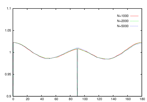
Figure 1: The lattice effect function using $80$ million samples. Three curves are shown for $N=1000,2000,5000$. Each curve is rescaled so it has average $1$.

5 Simulation tests of the predictions

We use the pivot algorithm to simulate the ensemble of SAW’s with a fixed number of steps. We use Clisby’s implementation of this algorithm which has dramatically increased its speed [3]. For all our simulations we plot the cumulative distribution function (CDF) rather than the density. Finding the density from a simulation requires taking a numerical derivative and so adds further uncertainty. As can be seen in figure 2 in [14], if we plot the predicted CDF and the CDF found in the simulation, the difference between them is too small to be seen in such a plot. So in this paper we only plot the differences - the simulation CDF minus the predicted CDF.

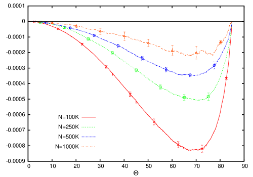
Figure 2: The curves are the difference between the simulation CDF’s for the hitting density for the half-space and the predicted CDF given by eq. (4). Four differences are shown corresponding to $N=100K,250K,500K,1000K$.

The first prediction we test is the hitting density for the SAW in the half-space $z<1$ starting at the origin and ending on the plane $z=1$. As discussed in section 3.1 we can study this ensemble by using the pivot algorithm to generate samples of the half-space fixed-length ensemble. This ensemble consists of all SAW’s with $N$ steps which start at the origin and stay in the half-space $z>0$. For any such SAW we can dilate it and translate it to produce a SAW in the half-space $z<1$ that goes between the origin and the plane $z=1$. As discussed in section 3.1, if we weight the SAW $\omega$ by $z(\omega)^{(\rho-\gamma)/\nu}$ then we expect the scaling limit to be the same as the scaling limit of the SAW in the half-space $z<1$ which start at the origin and end on the plane $z=1$. Here $z(\omega)$ is the $z$-component of the endpoint of the walk. When the SAW $\omega$ ends close to the plane $z=0$, $z(\omega)$ will be relatively small. Such SAW’s are improbable, but the weighting factor is large and so the statistical errors in the simulation are increased. The troublesome SAW’s typically have a value of $\theta$ near $90$ degrees. So if we only study the random variable $\theta$ for $\theta\leq\theta_{0}$ with $\theta_{0}$ slightly less than $90$, i.e., condition on $\theta\leq\theta_{0}$, we can reduce this problem. We take $\theta_{0}=85$.

We can compute $b$ using eq. 1 and the existing numerical estimates of the exponents $\rho,\gamma$ and $\nu$. However, the result is not accurate enough for our purposes. So we use our data for the half-space hitting density to estimate $b$ as follows. Let $F_{N}(\theta)$ be the CDF when we use $N$ step SAW’s, and let $H(\theta,b)$ be the predicted CDF. We assume that their difference is of the form

$$F_{N}(\theta)-H(\theta,b)\approx N^{-p}g(\theta)$$ (23)

where the function $g(\theta)$ and the power $p$ are unknown. Let $\beta$ be an initial estimate of $b$ and write $b=\beta+\epsilon$. So $\epsilon$ is small and we have

$$H(\theta,b)=H(\theta,\beta+\epsilon)\approx H(\theta,\beta)+\epsilon\frac{\partial H}{\partial\beta}(\theta,\beta)$$ (24)

So

$$F_{N}(\theta)-H(\theta,\beta)\approx N^{-p}g(\theta)+\epsilon\frac{\partial H}{\partial\beta}(\theta,\beta)$$ (25)

We compute the left side from our simulation and we also compute $\frac{\partial H}{\partial\beta}(\theta,\beta)$. We then use the data for the simulations with $N=100K,250K,500K$ to solve for $\epsilon,p$ and $g(\theta)$. We find $b=1.3303(3)$. The error bar given on this estimate is an educated guess obtained as follows. We find $p=0.538$. When we rescale the differences $F_{N}(\theta)-H(\theta,b)$ by $N^{p}$, the curves for different $N$ should collapse to a single curve. We obtain the error bar for $b$ by varying $b$ from our estimated value of $b=1.3303$ and seeing when this collapse clearly fails. A better method for studying the error in $b$ would be to run simulations for more values of $N$ and then use different sets of values of $N$ to estimate $b$.

Figure 2 shows the difference between the simulation CDF and the predicted CDF given by eq. (4) for the half-space for $N=100K,250K,500K$ and $1000K$. One of the most important features in this figure is the vertical scale. Even for the shortest length of $N=100K$, the maximum difference is only about $8\times 10^{-4}$. The error bars shown are plus or minus two standard deviations for the statistical errors in the simulation. They do not include the error from the finiteness of $N$. The figure shows that most of the difference comes from these finite $N$ errors, and these errors are going to zero as $N\rightarrow\infty$.

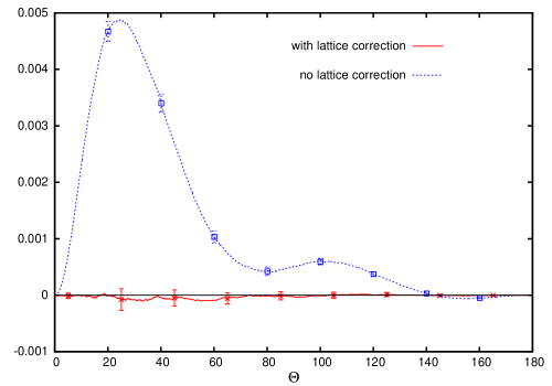
Figure 3: The curves are the difference between the simulation CDF’s using $N=1000K$ for the hitting density for a sphere centered at $(0,0,3/4)$ and the predicted CDF given by eq. (6). The curve that is nearly zero takes into account the lattice effect that survives the scaling limit, and the other curve does not.

The second prediction we test is the hitting density for the ensemble of SAW’s in the sphere of radius $1$ centered at the origin which have one endpoint at $(0,0,a)$ and the other endpoint on the surface of the sphere. We take $a=3/4$. As discussed in section 3.2 we use the fixed-length ensemble to study this hitting density. Given an $N$ step SAW in the full-space which starts at the origin, we dilate the walk to produce a walk with one endpoint at the origin and the other endpoint on the sphere of radius $1$ centered at $(0,0,-a)$. We then condition on the event that this dilated walk lies entirely inside the sphere. We weight the walk by $R(\omega)^{-(\gamma-\rho)/\nu}$, where $R(\omega)$ is the dilation factor. As we argued in section 3.1 we expect the scaling limit to be the same as the scaling limit of the SAW in the sphere. The lattice effects that were discussed in the previous section appear in this ensemble. They persist in the scaling limit and must be taken into consideration when we test our prediction for the hitting density. In figure 3 we plot the difference of the predicted CDF given by eq. (6) and the CDF from the simulation for $N=1,000K$. Two curves are shown. In one we take the lattice effect into account and in the other we do not. The figure shows that if we fail to account for the lattice effect, then the difference between the predicted CDF and the simulation CDF can be as large as $0.005$, much larger than the statistical errors in our simulations and the finite-$N$ errors.

The third prediction we test is for the ensemble of SAW’s in the full-space from $(0,0,0)$ to $(0,0,2)$. Our prediction for this ensemble gives the distribution of the point on the plane $z=1$ where the walk first hits the plane. We simulate this ensemble using the fixed-length ensemble. This ensemble consists of SAW in the full-space with $N$ steps which start at the origin. Given such a SAW we apply a Euclidean symmetry (rotation and dilation) that fixes the origin and take the other endpoint of the SAW to $(0,0,2)$. We weight the transformed $N$ step SAW $\omega$ by $||\omega(N)||^{-\gamma/\nu}$. As we argued in section 3.3 the scaling limit should be the same as the scaling limit of the ensemble of SAW’s from $(0,0,0)$ to $(0,0,2)$. In figure 4 we plot the differences between the simulation CDF and the predicted CDF given by eq. (7) for $N=100K,250K,500K,1000K$. Again the error bars are only for the statistical errors, and the figure shows the differences going to zero as $N\rightarrow\infty$.

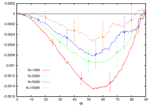
Figure 4: The curves are the difference between the simulation CDF’s for the first hit of the bisecting plane for a SAW between two points and the predicted CDF given by eq. (7). Four differences are shown corresponding to $N=100K,250K,500K,1000K$.

The pivot algorithm is a Markov chain Monte Carlo algorithm and so does not generate independent samples of the SAW. For the hitting density for the half-space and the distribution for the first hit of the bisecting plane, we sampled the Markov chain every 100 iterations. For $N=1000K$ we generated $10^{9}$ samples. For the smaller values of $N$ we generated on the order of $4\times 10^{9}$ samples. For the hitting density of the sphere we sampled the Markov chain every 10 iterations. However, in this simulation we must condition on the event that the dilated walk lies entirely in the sphere. The probability of this event goes to zero as $N\rightarrow\infty$. For $N=1000K$ the probability is approximately $0.0025$. To compensate for this small probability we generated $60\times 10^{9}$ samples.

6 Conclusions

We presented preliminary results on these tests of the conformal invariance of the three-dimensional SAW in [14]. The ensembles of SAW’s for which there are predictions based on conformal invariance have walks with varying lengths. However, the fastest computational method for the SAW, the pivot algorithm, studies an ensemble of walks which all have the same number of steps. A crucial tool in our study of these conformal invariance predictions is the method explained in section 3 of this paper that allows us to study the ensembles that involve walks of varying lengths using the fixed-length ensemble.

As in two dimensions, there are lattice effects that persist in the scaling limit that must be taken into account in our study of the prediction of the hitting density for the sphere. The computation of this lattice effect was discussed in section 4 of this paper.

For all three of our tests of the predictions of conformal invariance the simulations presented in this paper show excellent agreement. With $N=1000K$ the maximum differences between the predicted CDF’s and the CDF’s found in the simulations range from $1\times 10^{-4}$ to $6\times 10^{-4}$. The differences we see are due both to statistical errors and the finite length of the walks we use. For two of the three predictions we have presented simulations for several values of $N$, the length of the SAW, which clearly show the finite-$N$ error going to zero as $N\rightarrow\infty$.

Acknowledgments: The support of the Mathematical Science Research Institute in Berkeley, California where this research was begun is gratefully acknowledged. An allocation of computer time from the UA Research Computing High Performance Computing (HPC) and High Throughput Computing (HTC) at the University of Arizona is gratefully acknowledged.

References

- [1] D. Brydges, G. Slade, Renormalisation group analysis of weakly self-avoiding walk in dimensions four and higher, in Proceedings of the International Congress of Mathematicians (ed. R. Bhatia et al.), 4, 2232–2257 (2010).
- [2] J. Cardy, Conformal invariance and surface critical behavior, Nuc. Phys. B, 240, 514–532, (1984).
- [3] N. Clisby, Efficient implementation of the pivot algorithm for self-avoiding walks, J. Stat. Phys. 140, 349-392 (2010). Archived as arXiv:1005.1444v1 [cond-mat.stat-mech].
- [4] N. Clisby, Accurate estimate of the critical exponent for self-avoiding walks via a fast implementation of the pivot algorithm, Phys. Rev. Lett. 5, 55702 (2010). Archived as arXiv:1002.0494 [cond-mat.stat-mech].
- [5] B. Dyhr, M. Gilbert, T. Kennedy, G.F. Lawler, S. Passon, The self-avoiding walk in a strip, J. Stat. Phys. 144, 1 (2011). Archived as arXiv:1008.4321 [math.PR].
- [6] P. Flory, The configuration of real polymer chains, J. Chem. Phys., 17, 303 (1949).
- [7] T. Hara, G. Slade, Self-avoiding walk in five or more dimensions I. The critical behaviour, Commun. Math. Phys. 147, 101–136 (1992).
- [8] T. Hara, G. Slade, The lace expansion for self-avoiding walk in five or more dimensions, Rev. Math. Phys., 4, 235–327 (1992).
- [9] P. Grassberger, Simulations of grafted polymers in a good solvent, J. Phys. A 38, 323 (2005). Archived as arXiv:cond-mat/0410055 [cond-mat.soft].
- [10] T. Kennedy, Monte Carlo tests of SLE predictions for 2D self-avoiding walks, Phys. Rev. Lett. 88, 130601 (2002). Archived as arXiv:math/0112246v1 [math.PR].
- [11] T. Kennedy, Conformal invariance and stochastic Loewner evolution predictions for the 2D self-avoiding walk - Monte Carlo tests, J. Stat. Phys. 114, 51–78 (2004). Archived as arXiv:math/0207231v2 [math.PR].
- [12] T. Kennedy, G. Lawler, Lattice effects in the scaling limit of the two-dimensional self-avoiding walk, Fractal Geometry and Dynamical Systems in Pure and Applied Mathematics II: Fractals in Applied Mathematics 195–210, Contemporary Mathematics 601, Amer. Math. Soc., Providence, RI, 2013. Archived as arXiv:1109.3091v1 [math.PR].
- [13] T. Kennedy, Simulating self-avoiding walks in bounded domains, J. Math. Phys. 53, 095219 (2012). Archived as arXiv:1110.4167 [math.PR].
- [14] T. Kennedy, Conformal invariance of the 3D self-avoiding walk, Phys. Rev. Lett. 111, 165703 (2013). Archived as arXiv:1310.6979 [math-ph].
- [15] G. Lawler, O. Schramm, and W. Werner, On the scaling limit of planar self-avoiding walk, Fractal Geometry and Applications: a Jubilee of Benoit Mandelbrot, Part 2, 339–364, Proc. Sympos. Pure Math. 72, Amer. Math. Soc., Providence, RI, 2004. Archived as arXiv:math/0204277v2 [math.PR].
- [16] N. Madras and G. Slade, The Self-Avoiding Walk. Birkhäuser (1996).
- [17] B. Nienhuis, Exact critical point and critical exponents of models in two dimensions, Phys. Rev. Lett. 49, 1062–1065 (1982).
- [18] R. Schram, G. Barkema, R. Bisseling, Exact enumeration of self-avoiding walks, Journal of Statistical Mechanics: Theory and Experiment, 6, P06019 (2011). Archived as arXiv:1104.2184 [math-ph].