Abstract

This paper mainly focuses on studying the Shannon Entropy and Kullback-Leibler divergence of the multivariate log canonical fundamental skew-normal (LCFUSN) and canonical fundamental skew-normal (CFUSN) families of distributions, extending previous works. We relate our results with other well known distributions entropies. As a byproduct, we also obtain the Mutual Information for distributions in these families. Shannon entropy is used to compare models fitted to analyze the USA monthly precipitation data. Kullback-Leibler divergence is used to cluster regions in Atlantic ocean according to their air humidity level.

Keywords: multivariate log skew-normal; shannon entropy; kullback leibler divergence

AMS 1991 subject classification:62B10; 62F15

1 Introduction

In recent years, the interest in new parametric distributions able to model skewness, heavy tails, bimodality and some other data characteristics that are not well fitted by the usual distributions is growing. Seeking for flexible and tractable distributions to model non-negative data and motivated by some results that recently appeared in [23], the multivariate log-canonical fundamental skew-normal (LCFUSN) family of distributions is introduced in [22]. Our purpose in this work is to explore some properties of the LCFUSN family that are useful to solve relevant problems, such as the quantification of the information in a system or the definition of optimal designs. These types of problems can be addressed with information theory techniques, such as Shannon entropy or differential entropy (see [25]) and Kullback-Leibler (KL) divergence (see [18, 17]).

The Shannon entropy $H_{\bf Z}$ (hereafter, named entropy) of a continuous random vector ${\bf Z}\in\mathbb{R}^{n}$ can be understood as the mean information needed in order to describe the behavior of ${\bf Z}$ whereas the KL divergence measures the inefficiency in assuming that the distribution is $f_{{\bf Y}}$ when the true one is $f_{{\bf X}}$, that is, it measures the information lost when $f_{{\bf Y}}$ is used to approximate $f_{{\bf X}}$. The KL divergence between $f_{{\bf X}}$ and $f_{{\bf Y}}$, denoted by $D(f_{{\bf X}}||f_{{\bf Y}})$, is non-negative but it does not define a proper distance measure since it is not symmetric. A particular case of the KL divergence is the mutual information (MI) (see [25]) between the random vectors ${\bf X}\in\mathbb{R}^{n}$ and ${\bf Y}\in\mathbb{R}^{m}$, which is given by $I_{{\bf X},{\bf Y}}=D(f_{{\bf X},{\bf Y}}({\bf x},{\bf y})||f_{{\bf X}}({\bf x})f_{{\bf Y}}({\bf y}))$. Therefore, the MI measures the association between ${\bf X}$ and ${\bf Y}$ and is a useful tool to obtain information about the correlation of such quantities. It also follows that $I_{{\bf X},{\bf Y}}=I_{{\bf Y},{\bf X}}$ and $I_{{\bf X},{\bf Y}}=0$ if and only if ${\bf X}$ and ${\bf Y}$ are independent. The MI can also be obtained in terms of the entropies of ${\bf X}$ and ${\bf Y}$ through the simple relation

$$I_{{\bf X},{\bf Y}}=H_{{\bf X}}+H_{{\bf Y}}-H_{{\bf X}{\bf Y}}.$$ (1)

Additional details on this concepts can be found in [9].

The entropy of many distributions are already known. In [17] the authors obtained the entropy of a normal distribution while in [1] the entropies of several multivariate distributions are derived. In [12] and [13] the MI for non normal multivariate location scale families is studied. In [2] the authors obtained the entropy and MI in the multivariate elliptical and skew-elliptical families of distributions and applied their results to define an optimal design for an ozone monitoring station network. More recently, strategies to compute the KL and Jeffreys divergences in a class of multivariate SN distributions are proposed in [8].

Some information theory concepts have also been considered in Bayesian Statistics. For instance, the maximization of the entropy to build non informative prior distributions for the parameters is considered in [15]. In [7] the authors obtained the so-called reference prior, which corresponds to the Jeffreys prior in some particular cases, by maximizing the MI between the data ${\bf X}$ and the parameter $\theta$. In another direction, when the parametric form of the likelihood can not be identified, $I_{{\bf X},\mbox{\boldmath$\theta$}}$ is minimized in [26] in order to obtain the minimally informative likelihood function. In [21] the authors considered the KL divergence to assess the influence of model assumptions in the analysis. A loss function based on KL divergence to build a criterion for model selection is considered in [24]. More recently, in [11] it is proved that the natural conjugate prior distribution is maximally informative when it minimizes $I_{{\bf X},\mbox{\boldmath$\theta$}}$. Also, in [10] the Bayes estimator for the entropy by minimizing the expected Bergman divergence is obtained.

In this paper, we mainly focus on studying the entropy of the multivariate LCFUSN family of distribution, as well as the canonical fundamental skew-normal (CFUSN) distribution defined in [3]. As byproducts, we obtain the entropy of the multivariate log-skew-normal (LSN) distribution (see [20]) and generalize some results obtained in [2] for distributions with normal kernels. We obtain the relationship between the entropies of the multivariate LCFUSN and CFUSN distributions and some related distributions such as the multivariate normal, multivariate SN (see [6]) and the multivariate log-normal (LN) distributions. We also obtain the KL divergence to evaluate the “distance” between distributions in the CFUSN family as well as in LCFUSN family and also between the LCFUSN distribution and the LSN distribution. Some results related to the calculus of the entropy of some univariate LN and LSN distributions are also shown. To illustrate our results, we apply entropy to compare some log-skewed models fitted to analyze the USA monthly precipitation data. We also apply the KL divergence to cluster regions in Atlantic ocean according to their air humidity level.

This work is organized as follows. In Section 2 we present all univariate and multivariate distributions that are considered in this paper. In Section 3, we find the entropy of such distributions and obtain the relationship between them. We also derive the KL divergence and the MI for the LCFUSN and CFUSN families of distributions and, as a consequence, for the multivariate LSN distribution. In Section 4, some issues on Bayesian inference in the LCFUSN family are discussed and we analyse two procedures to estimate its entropy and KL divergence. To illustrate our results, we present two data analysis in Section 5. We also perform an analysis of simulated data sets comparing the fitting quality provided by LCFUSN, LN and LSN distributions. In Section 6, some conclusions and final comments close the paper.

Along the paper, $\phi_{n}({\bf x}|\mbox{\boldmath$\mu$},\mbox{\boldmath$\Sigma$})$ and $\Phi_{n}({\bf x}|\mbox{\boldmath$\mu$},\mbox{\boldmath$\Sigma$})$ denote the pdf and cumulative distribution function (cdf) of the multivariate normal distribution $N_{n}(\mbox{\boldmath$\mu$},\mbox{\boldmath$\Sigma$})$, respectively. If $\mbox{\boldmath$\mu$}=0$ such pdf and cdf are denoted by $\phi_{n}({\bf x}|\mbox{\boldmath$\Sigma$})$ and $\Phi_{n}({\bf x}|\mbox{\boldmath$\Sigma$})$ and, if in addition $\mbox{\boldmath$\Sigma$}=\mathbf{I}_{n}$, we write $\phi_{n}({\bf x})$ and $\Phi_{n}({\bf x})$, respectively. Also, denote by ${\bf{1}}_{n,m}$ and ${\bf{1}}_{n}$ the matrices of ones of order $n\times m$ and $n\times 1$, respectively.

2 Definitions and Preliminary Results

The distributions considered in the paper and some of its properties are presented in this section. Although some of them are completely standard, we show them for the benefit of the text. We begin with the construction of the LN distribution, since a similar idea is considered to build some other log-style distributions. It is well-known that if $X\sim N(\mu,\sigma^{2})$ and $Y=\exp(X)$ then $Y$ has LN distribution with parameters $\mu$ and $\sigma^{2}$, denoted by $Y\sim LN(\mu,\sigma^{2})$, with pdf given by $f(y\mid\mu,\sigma)=\frac{1}{y}\phi\left(\ln y|\mu,\sigma\right),\ y\in\mathbb{R}^{+}.$

Although usual, normality is not always a reasonable assumption in data analysis if, for instance, the data have a certain amount of asymmetry or the presence of heavy tails is realistic. In [4] the univariate SN distribution was introduced by multiplying the pdf of a normal distribution by a skewing function, which includes an additional parameter to control asymmetry. We say that $X\sim SN(\mu,\sigma,\alpha)$, where $\mu$, $\sigma^{2}$ and $\alpha\in\mathbb{R}$ are, respectively, the location, scale and shape parameters, if its pdf is given by

$$f(z\mid\mu,\sigma,\alpha)=\frac{2}{\sigma}\phi\left(\frac{z-\mu}{\sigma}\right)\Phi\left(\alpha\left(\frac{z-\mu}{\sigma}\right)\right),\ z\in\mathbb{R}.$$ (2)

The normal and the half-normal distributions are particular cases of Equation (2) when $\alpha$ equals zero and $\alpha\rightarrow\infty$, respectively. The expected value and variance of $X\sim SN(\mu,\sigma,\alpha)$ are given, respectively, by

$$E(X)=\mu+\sigma\sqrt{\frac{2}{\pi}}\frac{\alpha}{\sqrt{1+\alpha^{2}}}\mbox{ and }Var(X)=\sigma^{2}\left(1-\frac{2\alpha^{2}}{\pi(1+\alpha^{2})}\right).$$ (3)

Following ideas used in the normal case, the LSN distribution is introduced in [5]. Let Z $\sim$ SN($\mu,\sigma,\alpha$) and consider the transformation $Y=\exp(Z)$. Then Y has the LSN distribution, denoted by $Y\sim LSN(\mu,\sigma,\alpha)$, with pdf given by

$$f(y\mid\mu,\sigma,\alpha)=\frac{2}{\sigma y}\phi\left(\frac{\ln y-\mu}{\sigma}\right)\Phi\left(\alpha\left(\frac{\ln y-\mu}{\sigma}\right)\right),y\in\mathbb{R}^{+},$$ (4)

where $\mu\in\mathbb{R}$ is the location parameter, $\sigma^{2}>0$ is the scale parameter and $\alpha\in\mathbb{R}$ is the shape parameter. As before, if $\alpha=0$, then Equation (4) reduces to the LN distribution $LN(\mu,\sigma^{2})$.

The multivariate analog of the SN distribution was introduced in [6] and it is a particular case of the CFUSN family of distributions introduced in [3]. We say that ${\bf Z}$ has a $n$-variate CFUSN distribution with a $n\times m$ skewness matrix $\Delta$, which will be denoted by ${\bf Z}\sim CFUSN_{n,m}(\mbox{\boldmath$\Delta$})$, if its pdf is given by

$$f_{{\bf Z}}(\mathbf{z})=2^{m}\phi_{n}(\mathbf{z})\Phi_{m}(\mbox{\boldmath$\Delta$}^{\prime}\mathbf{z}|{\bf{I}}_{m}-\mbox{\boldmath$\Delta$}^{\prime}\mbox{\boldmath$\Delta$}),\,\,\,\,\mathbf{z}\in\mathbb{R}^{n},$$ (5)

where $\Delta$ is such that ${\bf{I}}_{m}-\mbox{\boldmath$\Delta$}^{\prime}\mbox{\boldmath$\Delta$}$ is a positive definite matrix, i.e, $||\mbox{\boldmath$\Delta$}\mathbf{a}||<1$, for all unitary vectors $\mathbf{a}\in\mathbb{R}^{m}$. Here $||^{.}||$ denotes euclidean norm. If $m=1$ and $\mbox{\boldmath$\Delta$}=(\delta_{1},\delta_{2},\dots,\delta_{n})^{\prime}$, then we obtain the multivariate SN family of distributions. Also, if $m=n$ and $\mbox{\boldmath$\Delta$}=\hbox{diag}(\delta_{1},\delta_{2},\dots,\delta_{n})$, then Equation (5) reduces to the product of $n$ SN marginal distributions. Consequently, for any random sample of the univariate SN distribution $Y_{i}\sim SN(\alpha)$, $i=1,\dots,n$, we have ${\bf Y}=(Y_{1},\dots,Y_{n})^{\prime}\sim CFUSN_{n,n}(\delta{\bf{I}}_{n})$, where $\delta=\alpha[1+\alpha^{2}]^{-1/2}$.

In [3] a location scale version of the CFUSN distribution is introduced. This is accomplished by considering ${\bf Z}\sim CFUSN_{n,m}(\mbox{\boldmath$\Delta$})$ and the linear transformation ${\bf W}=\mbox{\boldmath$\mu$}+\mbox{\boldmath$\Sigma$}^{1/2}{\bf Z}$, where $\mu$ is the location vector of order $n\times 1$ and $\Sigma$ denotes the definite positive scale matrix of dimension $n\times n$. We say that ${\bf W}\sim CFUSN_{n,m}(\mbox{\boldmath$\mu$},\mbox{\boldmath$\Sigma$},\mbox{\boldmath$\Delta$})$ if its pdf is

$$f_{{\bf W}}({\bf w}) = 2^{m}|\mbox{\boldmath$\Sigma$}|^{-1/2}\phi_{n}(\mbox{\boldmath$\Sigma$}^{-1/2}({\bf w}-\mbox{\boldmath$\mu$}))$$ (6)

$$\times \Phi_{m}(\mbox{\boldmath$\Delta$}^{\prime}\mbox{\boldmath$\Sigma$}^{-1/2}({\bf w}-\mbox{\boldmath$\mu$})|\mbox{\boldmath$I$}_{m}-\mbox{\boldmath$\Delta$}^{\prime}\mbox{\boldmath$\Delta$}),{\bf w}\in\mathbb{R}^{n},$$

where $|\mathbf{A}|$ stands for $det\,(\mathbf{A})$.

If data has positive support, the use of distributions with real support to describe their behavior cannot be appropriate. In the univariate case there are many different distributions that are useful to that purpose. However, multivariate versions of such univariate distributions are usually intractable. In [22] the authors introduced the LCFUSN family of distributions in the following way. Let ${\bf Z}=(Z_{1},\dots,Z_{n})^{\prime}$ be a $n\times 1$ random vector and consider the transformations ${\exp({\mathbf{Z}})}=(\exp(Z_{1}),\dots,\exp(Z_{n}))^{\prime}$ and ${\ln{\mathbf{Z}}}=(\ln Z_{1},\dots,\ln Z_{n})^{\prime}$. Hereafter we assume that $\mbox{\boldmath$\Delta$}^{*}={\bf{I}}_{m}-\mbox{\boldmath$\Delta$}^{\prime}\mbox{\boldmath$\Delta$}$.

Definition 1

Let ${\bf Y}$ and ${\bf Z}=\ln{\bf Y}$ be $n\times 1$ random vectors. If $\mathbf{Z}\sim CFUSN_{n,m}(\mathbf{\Delta})$, we say that ${\bf Y}$ has a log-canonical fundamental skew-normal distribution with skewness matrix $\mathbf{\Delta}$ denoted by $\mathbf{Y}\sim LCFUSN_{n,m}(\mathbf{\Delta})$. The pdf of $\mathbf{Y}$ is

$$f_{\mathbf{Y}}(\mathbf{y})=2^{m}\left(\prod_{i=1}^{n}y_{i}\right)^{-1}\phi_{n}(\ln\mathbf{y})\Phi_{m}(\mathbf{\Delta}^{\prime}\ln\mathbf{y}|\mbox{\boldmath$\Delta$}^{*}),\,\,\,\,\mathbf{y}\in\mathbb{R}^{n^{+}},$$ (7)

where $\mathbf{\Delta}$ is a $n\times m$ matrix such that $||\mathbf{\Delta}\textbf{a}||<1$, for all unity vectors a $\in\mathbb{R}^{m}$.

The location-scale version of the LCFUSN distribution is obtained by considering a $n\times 1$ random vector ${\bf W}\sim CFUSN_{n,m}(\mbox{\boldmath$\mu$},\mbox{\boldmath$\Sigma$},\mbox{\boldmath$\Delta$})$ and the transformation $\mathbf{U}=\exp({\bf W})$. In this case, the pdf of $\mathbf{U}\sim LCFUSN_{n,m}(\mbox{\boldmath$\mu$},\mbox{\boldmath$\Sigma$},\mbox{\boldmath$\Delta$})$ is

$$f_{{\bf U}}({\bf u})=\frac{2^{m}|\mbox{\boldmath$\Sigma$}|^{-1/2}}{\prod_{j=1}^{n}u_{j}}\phi_{n}(\mbox{\boldmath$\Sigma$}^{-1/2}(\ln{\bf u}-\mbox{\boldmath$\mu$}))\Phi_{m}(\mbox{\boldmath$\Delta$}^{\prime}\mbox{\boldmath$\Sigma$}^{-1/2}(\ln{\bf u}-\mbox{\boldmath$\mu$})|\mbox{\boldmath$\Delta$}^{*}),$$ (8)

for all $\mathbf{u}\in\mathbb{R}^{n^{+}}$, where $\mu$ is a $n\times 1$ location vector, $\Sigma$ a $n\times n$ definite positive scale matrix and $\Delta$ a skewness matrix. The LCFUSN family of distributions generalizes the multivariate LSN family defined in [20], which can be obtained from Equation (7) by taking $m=1$ and $\mbox{\boldmath$\alpha$}^{\prime}=(1-\mathbf{\Delta}^{\prime}\mathbf{\Delta})^{-\frac{1}{2}}\mathbf{\Delta}^{\prime}{\mbox{\boldmath$\Sigma$}}^{-\frac{1}{2}}{\mbox{\boldmath$\omega$}}$, where ${\mbox{\boldmath$\omega$}}=diag({\mbox{\boldmath$\Sigma$}})^{\frac{1}{2}}$ is a $n\times n$ scale matrix.

3 Information Theory in the CFUSN and LCFUSN Distributions

In this section we calculate the entropy and the KL divergence for the multivariate CFUSN and the multivariate LCFUSN families of distributions and associate them to the entropy of related distributions. We start with the univariate case and obtain the entropy of the LSN distribution (see [5]) and its relationship with the normal, SN and LN entropies.

3.1 Univariate Cases

It is well-known that the maximum entropy among all univariate continuous symmetric distributions is observed for the normal distribution (see [9]). If $X\sim N(\mu,\sigma^{2})$, then the entropy of $X$ is

$$H_{N(\mu,\sigma^{2})}=\frac{1}{2}\ln\sigma^{2}+\frac{1}{2}(1+\ln(2\pi)),$$ (9)

which increases with the variance of the distribution. Opposed to what is observed for $H_{N(\mu,\sigma^{2})}$, the entropy of a LN distribution also depends on the location parameter $\mu$. Formally, if $X\sim LN(\mu,\sigma^{2})$, then

$$H_{LN(\mu,\sigma^{2})}=H_{N(\mu,\sigma^{2})}+\mu.$$ (10)

The entropy of a LN distribution is an increasing function of $\mu$ and is higher than the entropy of $N(\mu,\sigma^{2})$ if and only if $\mu>0$. In [2] the entropy of the multivariate skew-elliptical class of distributions is obtained. Particularly, they show that the entropy of $X\sim SN(\mu,\sigma^{2},\alpha)$, a special case of such a class, is a function of the entropy of the $N(\mu,\sigma^{2})$ distribution and is given by

$$H_{SN(\mu,\sigma^{2},\alpha)}=H_{N(\mu,\sigma^{2})}-E_{X_{0}}[\ln(2\Phi(\alpha X_{0}))],$$ (11)

where $X_{0}\sim SN(\alpha)$. As expected, if $\alpha=0$, we have that $H_{SN(\mu,\sigma^{2},\alpha)}=H_{N(\mu,\sigma^{2})}$. Moreover, it follows from the monotone convergence theorem that

$$\lim_{\alpha\to\pm\infty}H_{SN(\mu,\sigma^{2},\alpha)}=H_{N(\mu,\sigma^{2})}-\ln(2).$$ (12)

As far as we know, the next result is new and provides the entropy of the LSN distribution.

Proposition 1

If $Y\sim LSN(\mu,\sigma^{2},\alpha)$ then the entropy of $Y$ is

$$H_{LSN(\mu,\sigma^{2},\alpha)}=H_{SN(\mu,\sigma^{2},\alpha)}+E(X),$$ (13)

where $X\sim SN(\mu,\sigma^{2},\alpha)$ and $E(X)$ is given in Equation (3).

The proof of Proposition 1 follows by noticing that $\ln f_{Y}(Y)\buildrel d\over{=}-X+\ln f_{X}(X)$, where $X\sim SN(\mu,\sigma^{2},\alpha)$. Besides, the relationship between the entropies of the LSN, LN and normal distributions follows immediately from results in Equations (10) and (11). The entropy in Equation $(\ref{entrologskew})$ can be written as $H_{LSN(\mu,\sigma^{2},\alpha)}=H_{N(\mu,\sigma^{2})}-E[\ln(2\Phi(\alpha X_{0}))]+E(X)$ and $H_{LSN(\mu,\sigma^{2},\alpha)}=H_{LN(\mu,\sigma^{2})}-E[\ln(2\Phi(\alpha X_{0}))]+\mu+E(X),$ where $X\sim SN(\mu,\sigma^{2},\alpha)$ and $X_{0}\sim SN(\alpha)$. Moreover, from Equations (3) and (12),

$$\lim_{\alpha\to{\pm\infty}}H_{LSN(\mu,\sigma^{2},\alpha)} = H_{N(\mu,\sigma^{2})}+\mu\pm\sigma\sqrt{\frac{2}{\pi}}-\ln(2).$$

Also, if $\alpha=0$ in Equation (13), then $H_{LSN(\mu,\sigma^{2},\alpha)}=H_{LN(\mu,\sigma^{2})}.$

Figure 1: Entropy of the $SN(0,\sigma^{2},\alpha)$ (left) and $LSN(0,\sigma^{2},\alpha)$ (right) for $\sigma^{2}=0.5$ (dotted line), $1$ (solid line) and $1.5$(dotted-dashed line).

Figure 1 displays the entropies of $SN(0,\sigma^{2},\alpha)$ and $LSN(0,\sigma^{2},\alpha)$ as a function of the skewness parameter $\alpha$. The expectations involved in their computation were approximated using Monte Carlo methods. Figure 1 suggests that $H_{LSN(\mu,\sigma^{2},\alpha)}$ is an increasing function of $\alpha$ until a global maximum $H_{LSN(\mu,\sigma^{2},\alpha^{*})}$ and decreasing afterwards. A similar behavior is observable for $H_{SN(\mu,\sigma^{2},\alpha)}$. Also, we note that the curve of $H_{SN(\mu,\sigma^{2},\alpha)}$ has a symmetric shape and if we increase $\sigma^{2}$ by one unity it is translated by a factor of $\ln(\sigma^{2}+1)$.

3.2 Multivariate cases

In this section we obtain the entropies of the CFUSN and LCFUSN distributions and their connections with the entropies of a multivariate normal, multivariate SN and multivariate LSN (see [6] and [20]) distributions. We extend some results obtained in [2] for distributions with normal kernel.

Let ${\bf Z}$ be a $n$-dimensional random vector such that ${\bf Z}\sim N_{n}(\mbox{\boldmath$\mu$},\mbox{\boldmath$\Sigma$})$. The entropy of ${\bf Z}$ is

$$H_{N_{n}(\mbox{\boldmath$\mu$},\bf{\Sigma})}=\frac{1}{2}\ln|\mbox{\boldmath$\Sigma$}|+\frac{n}{2}(1+\ln(2\pi))=\frac{1}{2}\ln|\mbox{\boldmath$\Sigma$}|+H_{N_{n}({\bf{0}},{\bf{I}}_{n})},$$ (14)

where $H_{N_{n}({\textbf{0}},{\bf{I}}_{n})}=\frac{n}{2}(1+\ln(2\pi))$ is the entropy of a random vector with standard $n$-variate normal distribution. As in the univariate case, $H_{N_{n}(\mbox{\boldmath$\mu$},\bf{\Sigma})}$ does not depend on the location parameter $\mu$.

The CFUSN family is a more general class of skewed distributions with normal kernel. In [3] many of its properties are obtained. In particular, it is shown that if ${\bf X}\sim CFUSN_{n,m}(\mbox{\boldmath$\mu$},\mbox{\boldmath$\Sigma$},\mathbf{\Delta})$ then

$$E({\bf X})=\mathbf{\mbox{\boldmath$\mu$}}+\sqrt{\frac{2}{\pi}}\mbox{\boldmath$\Sigma$}^{1/2}\mbox{\boldmath$\Delta$}\mathbf{1}_{m},\,\,\,\,\,\,Var({\bf X})=\mbox{\boldmath$\Sigma$}-\frac{2}{\pi}\mbox{\boldmath$\Sigma$}^{1/2}\mbox{\boldmath$\Delta$}\mbox{\boldmath$\Delta$}^{\prime}\mbox{\boldmath$\Sigma$}^{1/2}.$$ (15)

They also prove that if $({\bf X}_{1},\dots,{\bf X}_{n})$ and $(\mbox{\boldmath$\Delta$}_{1},\dots,\mbox{\boldmath$\Delta$}_{n})$ are partitions of ${\bf X}\sim CFUSN_{n,m}{(\mbox{\boldmath$\Delta$})}$ and $\Delta$ respectively, then $X_{i}\sim CFUSN_{1,m}(\mbox{\boldmath$\Delta$}_{i})$, $i=1,\dots,n$. Despite their great contribution, the authors in [3] do not obtain results related to the entropy in the CFUSN family. In the next proposition we provide an expression for this entropy. Proof is given in Appendix.

Proposition 2

If ${\bf X}\sim CFUSN_{n,m}(\mbox{\boldmath$\mu$},\mbox{\boldmath$\Sigma$},\mbox{\boldmath$\Delta$})$, then the entropy of the canonical fundamental skew normal random vector ${\bf X}$ is

$$H_{CFUSN(\mbox{\boldmath$\mu$},\bf{\Sigma},\bf{\Delta})} = H_{N_{n}(\bf{0},\bf{I_{n}})}+\frac{1}{2}\ln|\mbox{\boldmath$\Sigma$}|+\frac{1}{\pi}[\mathbf{1}_{m}^{{}^{\prime}}\mbox{\boldmath$\Delta$}^{{}^{\prime}}\mbox{\boldmath$\Delta$}\mathbf{1}_{m}-tr(\mbox{\boldmath$\Delta$}\mbox{\boldmath$\Delta$}^{{}^{\prime}})]$$

$$- E_{{\bf X}_{0}}[\ln(2^{m}\Phi_{m}(\mbox{\boldmath$\Delta$}^{\prime}{\bf X}_{0}|\mbox{\boldmath$\Delta$}^{*}))]$$

where ${\bf X}_{0}\sim CFUSN_{n,m}(\mbox{\boldmath$\Delta$})$.

Some interesting results are obtained for particular structures of the scale $\Sigma$ and the skewing $\Delta$ matrices. If $\Sigma$ is a covariance matrix, the relationship between $H_{N_{n}(\mbox{\boldmath$\mu$},\bf{\Sigma})}$ and $H_{CFUSN(\mbox{\boldmath$\mu$},\bf{\Sigma},\bf{\Delta})}$ follows from Equations (14) and (2) . If in addition $\mbox{\boldmath$\Delta$}\mbox{\boldmath$\Delta$}^{{}^{\prime}}$ is diagonal, then the entropy in Equation (2) is simplified to

$$H_{CFUSN_{n,m}(\mbox{\boldmath$\mu$},\mathbf{\Sigma},\mathbf{\Delta})}=H_{N_{n}(\mbox{\boldmath$\mu$},\bf{\Sigma})}-E[\ln(2^{m}\Phi_{m}(\mbox{\boldmath$\Delta$}^{\prime}{\bf X}_{0}|\mbox{\boldmath$\Delta$}^{*}))],$$ (17)

where $\mathbf{X}_{0}\sim CFUSN_{n,m}(\mbox{\boldmath$\Delta$})$. The result in Equation (17) generalizes those obtained in [2] for distributions with normal kernel, including the multivariate SN distribution defined in [6].

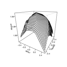
Figure 2 shows the entropy of the standard CFUSN family in the multivariate and univariate cases. We observe that the entropy is concave and presents symmetric behavior around zero. The maximum entropy is obtained when the skewing parameter is zero, that is, in the normal case. Besides, the entropy decay is smooth for small values of $m$. We also note that, for fixed $\Delta$, the smaller the value of $m$, the higher the entropy. Finally, the entropy tends to be closer to the normal entropy for values of $\Delta$ around zero.

Figure 2: Entropy of the $CFUSN_{1,2}(\mbox{\boldmath$\Delta$})$ with $\mbox{\boldmath$\Delta$}=(\delta_{1},\delta_{2})$ (left and middle) and the $CFUSN_{1,2}(\delta{\bf{1}}_{m})$(right).

In Proposition 3 we obtain the entropy of the LCFUSN distribution introduced in [22] which pdf is given in Equation (7).

Proposition 3

If ${\bf Z}\sim LCFUSN_{n,m}(\mbox{\boldmath$\mu$},\mbox{\boldmath$\Sigma$},\mbox{\boldmath$\Delta$})$, then the entropy of ${\bf Z}$ is

$$H_{LCFUSN_{n,m}(\mbox{\boldmath$\mu$},\bf{\Sigma},\bf{\Delta})}=H_{CFUSN_{n,m}(\mbox{\boldmath$\mu$},\bf{\Sigma},\bf{\Delta})}+\sum_{i=1}^{n}E(X_{i}),$$ (18)

where $X_{i}$ is the $ith$ component of the vector ${\bf X}\sim CFUSN_{n,m}(\mbox{\boldmath$\mu$},\mbox{\boldmath$\Sigma$},\mbox{\boldmath$\Delta$})$.

The proof of Proposition 3 is straightforward by noticing that if ${\bf X}\sim CFUSN(\mbox{\boldmath$\mu$},\bf{\Sigma},\bf{\Delta})$ then $\ln f_{{\bf Y}}({\bf Y})\buildrel d\over{=}\ln f_{{\bf X}}({\bf X})-{\bf{1}}_{n}^{{}^{\prime}}{\bf X}$. We can also rewrite the entropy in Equation (18) considering the results in Equation (15) and Proposition 2, obtaining

$$H_{LCFUSN_{n,m}(\mbox{\boldmath$\mu$},\bf{\Sigma},\bf{\Delta})}=H_{N_{n}(\bf{0},\bf{I_{n}})}+\frac{1}{2}\ln|\mbox{\boldmath$\Sigma$}|+\frac{1}{\pi}[\mathbf{1}_{m}^{{}^{\prime}}\mbox{\boldmath$\Delta$}^{{}^{\prime}}\mbox{\boldmath$\Delta$}\mathbf{1}_{m}-tr(\mbox{\boldmath$\Delta$}\mbox{\boldmath$\Delta$}^{{}^{\prime}})]$$ (19)

$$+ \sum_{i=1}^{n}\mu_{i}+\sqrt{\frac{2}{\pi}}{\bf 1}_{n}^{\prime}\mbox{\boldmath$\Sigma$}^{1/2}\mbox{\boldmath$\Delta$}\textbf{1}_{m}-E_{X_{0}}[\ln(2^{m}\Phi_{m}(\mbox{\boldmath$\Delta$}^{\prime}{\bf X}_{0}|\mbox{\boldmath$\Delta$}^{*}))],$$

where the random vector ${\bf X}_{0}\sim CFUSN_{n,m}(\mbox{\boldmath$\Delta$})$. If $\Sigma$ is a covariance matrix, the relationship between the LCFUSN and the non standard multivariate normal entropies follows from Equations (14) and (19) . If additionally $\mbox{\boldmath$\Delta$}^{{}^{\prime}}\mbox{\boldmath$\Delta$}$ is a diagonal matrix then we obtain

$$H_{LCFUSN_{n,m}(\mbox{\boldmath$\mu$},\bf{\Sigma},\mathbf{\Delta})} = H_{N_{n}(\mbox{\boldmath$\mu$},\mathbf{\Sigma})}+\sum_{i=1}^{n}\mu_{i}+\sqrt{\frac{2}{\pi}}{\bf 1}_{n}^{\prime}\mbox{\boldmath$\Sigma$}^{1/2}\mbox{\boldmath$\Delta$}\textbf{1}_{m}$$ (20)

$$- E_{{\bf X}_{0}}[\ln(2^{m}\Phi_{m}(\mbox{\boldmath$\Delta$}^{\prime}{\bf X}_{0}|\mbox{\boldmath$\Delta$}^{*}))],$$

where $\mathbf{}X_{0}\sim CFUSN_{n,m}(\mbox{\boldmath$\Delta$})$ and $\mu_{i}$ is the $i$th component of vector $\mu$.

The entropies of the multivariate LSN and the multivariate LN distributions are obtained easily from Proposition 3, since these distributions are special cases of the LCFUSN distribution.

Figure 3 shows the entropy of the univariate standard $LCFUSN_{1,2}(\mbox{\boldmath$\Delta$})$ as a function of $\Delta$. We assume two different structures for the skewness matrix $\Delta$. The plot on the right also shows the influence of $m$ in the entropy of a $LCFUSN_{1,m}(\delta{\bf{1}}_{m})$. It can be seen that the entropy of the LCFUSN increases with $\delta$ and is smooth for small values of $m$. Moreover, for $\delta<0$, the highest the value of $m$, the smallest the entropy. The opposite is observed if $\delta>0$.

Figure 3: Entropy of the $LCFUSN_{1,2}(\mbox{\boldmath$\Delta$})$ with $\mbox{\boldmath$\Delta$}=(\delta_{1},\delta_{2})$ (left and middle) and $\mbox{\boldmath$\Delta$}=$ $\delta{\bf{1}}_{m}$ (right).

3.3 KL Divergence and MI in the CFUSN and LCFUSN Families of Distributions

An useful tool to compare two distributions is the so called KL divergence. This quantity measures the inefficiency of assuming that the true distribution is $f_{{\bf X}}$ whereas it is $f_{{\bf Y}}$. In the next proposition we obtain the KL divergence in the CFUSN and LCFUSN families. It is remarkable that Proposition 4 provides the KL divergence for all families of distributions considered in this work. As can be seen below, the KL divergence is invariant under the exponential transformation.

Proposition 4

In the following cases:

• if ${\bf Z}\sim CFUSN_{n,m_{1}}(\mbox{\boldmath$\mu$}_{1},\mbox{\boldmath$\Sigma$}_{1},\mbox{\boldmath$\Delta$}_{1})$ and ${\bf Y}\sim CFUSN_{n,m_{2}}(\mbox{\boldmath$\mu$}_{2},\mbox{\boldmath$\Sigma$}_{2},\mbox{\boldmath$\Delta$}_{2})$ and

• if ${\bf Z}\sim LCFUSN_{n,m_{1}}(\mbox{\boldmath$\mu$}_{1},\mbox{\boldmath$\Sigma$}_{1},\mbox{\boldmath$\Delta$}_{1})$ and ${\bf Y}\sim LCFUSN_{n,m_{2}}(\mbox{\boldmath$\mu$}_{2},\mbox{\boldmath$\Sigma$}_{2},\mbox{\boldmath$\Delta$}_{2})$,

the KL divergence between ${\bf Y}$ and ${\bf Z}$ is given by

$$D(f_{{\bf Y}}||f_{{\bf Z}}) = \frac{1}{2}\ln\left[\frac{|\mbox{\boldmath$\Sigma$}_{1}|}{|\mbox{\boldmath$\Sigma$}_{2}|}\right]-\frac{n}{2}+E_{{\bf Y}}\left(\ln\left[\frac{2^{m_{2}-m_{1}}\Phi_{m_{2}}(\mbox{\boldmath$\Delta$}_{2}^{\prime}\mbox{\boldmath$\Sigma$}_{2}^{-\frac{1}{2}}({\bf Y}-\mbox{\boldmath$\mu$}_{2})|\mbox{\boldmath$\Delta$}_{2}^{*})}{\Phi_{m_{1}}(\mbox{\boldmath$\Delta$}_{1}^{\prime}\mbox{\boldmath$\Sigma$}_{1}^{-\frac{1}{2}}({\bf Y}-\mbox{\boldmath$\mu$}_{1})|\mbox{\boldmath$\Delta$}_{1}^{*})}\right]\right)$$ (21)

$$+ \frac{1}{2}[(\mbox{\boldmath$\mu$}_{1}-\mbox{\boldmath$\mu$}_{2})^{\prime}\mbox{\boldmath$\Sigma$}_{1}^{-1}(\mbox{\boldmath$\mu$}_{1}-\mbox{\boldmath$\mu$}_{2})+tr(\mbox{\boldmath$\Sigma$}_{1}^{-1}\mbox{\boldmath$\Sigma$}_{2})]$$

$$+ \frac{1}{\pi}[{\bf{W}}^{\prime}{\mbox{\boldmath$\Sigma$}}_{1}{\bf{W}}-tr(\mbox{\boldmath$\Sigma$}_{2}^{-1/2}{\mbox{\boldmath$\Delta$}}_{2}{\mbox{\boldmath$\Delta$}}_{2}^{{}^{\prime}}{\mbox{\boldmath$\Sigma$}}_{2}^{-1/2})-\mathbf{1}_{m_{2}}^{{}^{\prime}}\mbox{\boldmath$\Delta$}_{2}^{{}^{\prime}}\mbox{\boldmath$\Delta$}_{2}\mathbf{1}_{m_{2}}+tr(\mbox{\boldmath$\Delta$}_{2}\mbox{\boldmath$\Delta$}_{2}^{{}^{\prime}})]$$

$$+ \frac{1}{\sqrt{2\pi}}[({\mbox{\boldmath$\mu$}}_{2}^{\prime}-{\mbox{\boldmath$\mu$}}_{1}^{\prime}){\bf{W}}+{\bf{W}}^{\prime}({\mbox{\boldmath$\mu$}}_{2}-{\mbox{\boldmath$\mu$}}_{1})],$$

where ${\bf{W}}=\mbox{\boldmath$\Sigma$}_{1}^{-1}\mbox{\boldmath$\Sigma$}_{2}^{-1/2}\mbox{\boldmath$\Delta$}_{2}\mathbf{1}_{m_{2}}$ and $\mbox{\boldmath$\Delta$}_{i}^{*}={\bf{I}}_{m_{i}}-\mbox{\boldmath$\Delta$}_{i}^{\prime}\mbox{\boldmath$\Delta$}_{i}$.

The proof of item $(i)$ in Proposition 4 can be found in the appendix. Item $(ii)$ follows by observing that if ${\bf Z}\sim CFUSN_{n,m_{1}}(\mbox{\boldmath$\mu$}_{1},\mbox{\boldmath$\Sigma$}_{1},\mbox{\boldmath$\Delta$}_{1})$, ${\bf Y}\sim CFUSN_{n,m_{2}}(\mbox{\boldmath$\mu$}_{2},\mbox{\boldmath$\Sigma$}_{2},\mbox{\boldmath$\Delta$}_{2})$, $\bf U=\exp{({\bf Z})}$ and $\bf V=\exp{({\bf Y})}$, then

$$D(f_{{\bf U}}||f_{\bf V}) = E\left(\hbox{log}\frac{f_{\bf U}({\bf U})}{f_{\bf V}({\bf U})}\right)=E\left(\hbox{log}\frac{f_{\bf Z}(\hbox{log}\,{\bf U})}{f_{\bf Y}(\hbox{log}\,{\bf U})}\right)$$

$$= E\left(\hbox{log}\frac{f_{\bf Z}(\bf Z)}{f_{\bf Y}(\bf Z)}\right)=D(f_{\bf Z}||f_{\bf Y}).$$

The KL divergence between two $n$-variate normal distributions is obtained from Equation (21) by assuming $\mbox{\boldmath$\Delta$}_{1}$ and $\mbox{\boldmath$\Delta$}_{2}$ as null matrices. Proposition 4 also provides the KL divergence between the LSN and LCFUSN distributions. If we consider the parametrization of the LSN distribution assumed in [20], then Equation (21) becomes

$$D(f_{{\bf Y}}||f_{{\bf Z}})=E_{{\bf X}_{0}}\left[\ln\left(\frac{2^{m-1}\Phi_{m}(\mbox{\boldmath$\Delta$}{\bf X}_{0}|\mbox{\boldmath$\Delta$}^{*})}{\Phi(\mbox{\boldmath$\alpha$}^{\prime}\mbox{\boldmath$\omega$}^{-1}\mbox{\boldmath$\Sigma$}^{\frac{1}{2}}{\bf X}_{0})}\right)\right],$$

where ${\bf X}_{0}\sim CFUSN_{n,m}(\mbox{\boldmath$\Delta$})$, $\mbox{\boldmath$\alpha$}\in\mathbb{R}^{n}$ and ${\mbox{\boldmath$\omega$}}=diag(\mbox{\boldmath$\Sigma$})^{1/2}$.

Graphics displayed in Figure 4 disclose that, for fixed $\delta$, the KL divergence between $LCFUSN_{1,m}(\mbox{\boldmath$\Delta$})$ and $LSN_{1}(0,1,\alpha)$ increases as $m$ increases. Similar behavior is observed for fixed $m$ when $\delta$ is increasing and positive. Moreover, the KL divergence seems to be symmetric in $\delta$ at least in cases $m=2,3\mbox{ and }4$.

Figure 4: KL divergence between $LCFUSN_{1,m}(\mbox{\boldmath$\Delta$})$ and $LSN_{1}(0,1,\alpha)$ with $\mbox{\boldmath$\alpha$}^{\prime}=(1-\mbox{\boldmath$\Delta$}^{\prime}\mbox{\boldmath$\Delta$})^{-\frac{1}{2}}\mbox{\boldmath$\Delta$}^{\prime}$ and $\mbox{\boldmath$\Delta$}=$ $\delta{\bf{1}}_{m}$ .

Let ${\bf X}_{1}$ and ${\bf X}_{2}$ be a partition of ${\bf X}$. Suppose we want to quantify the amount of information ${\bf X}_{1}$ brings about ${\bf X}_{2}$ when ${\bf X}$ has distribution in the CFUSN or the LCFUSN family. Since these families are closed under marginalization (see [22, 3]), from Equation (1) we obtain

$$I_{{\bf X}_{1}{\bf X}_{2}}=E_{X}\left[\ln\left(\frac{\Phi_{m}(\mbox{\boldmath$\Delta$}^{\prime}{\bf X}|\mathbf{I}_{m}-\mbox{\boldmath$\Delta$}^{\prime}\mbox{\boldmath$\Delta$})}{2^{m}\Phi_{m}(\mbox{\boldmath$\Delta$}_{1}^{\prime}{\bf X}_{1}|\mathbf{I}_{m}-\mbox{\boldmath$\Delta$}_{1}^{\prime}\mbox{\boldmath$\Delta$}_{1})\Phi_{m}(\mbox{\boldmath$\Delta$}_{2}^{\prime}{\bf X}_{2}|\mathbf{I}_{m}-\mbox{\boldmath$\Delta$}_{2}^{\prime}\mbox{\boldmath$\Delta$}_{2})}\right)\right],$$ (22)

in the following cases:

• if ${\bf X}\sim CFUSN_{n,m}(\mbox{\boldmath$\Delta$})$, ${\bf X}_{1}\sim CFUSN_{n_{1},m}(\mbox{\boldmath$\Delta$}_{1})$ and ${\bf X}_{2}\sim CFUSN_{n_{2},m}(\mbox{\boldmath$\Delta$}_{2})$;

• if ${\bf X}\sim LCFUSN_{n,m}(\mbox{\boldmath$\Delta$})$, ${\bf X}_{1}\sim LCFUSN_{n_{1},m}(\mbox{\boldmath$\Delta$}_{1})$ and ${\bf X}_{2}\sim LCFUSN_{n_{2},m}(\mbox{\boldmath$\Delta$}_{2})$.

Observe that the MI on these families of distributions is also invariant under the exponential transformation, since it is a particular case of the KL divergence.

4 Bayesian Estimation of the LCFUSN Entropy

The entropy and the KL divergence depend on the parameters of the LCFUSN distribution and thus, under the Bayesian paradigm, are random quantities. In order to estimate such quantities it is necessary to obtain their posterior distributions, which can be a hard task if we search for closed expressions for them. However, good approximations can be obtained using MCMC methods. We only take into consideration particular univariate cases of the LCFUSN family since one of our goals in Section 5 is to evaluate the effect of increasing $m$ in data fitting. Similar strategy can be used in the multivariate case.

To achieve our goal, let $Y_{1},...,Y_{L}$ be a random sample of $Y\mid\mu,\sigma,\mbox{\boldmath$\Delta$}\buildrel iid\over{\sim}LCFUSN_{1,m}(\mu,\sigma^{2},\mbox{\boldmath$\Delta$})$, which induces the following likelihood function:

$$f({\bf y}|\mu,\sigma^{2},\mbox{\boldmath$\Delta$})=\frac{2^{Lm}\exp\left\{-\sum_{i=1}^{L}\frac{(\ln y_{i}-\mu)^{2}}{2\sigma^{2}}\right\}}{(2\pi\sigma^{2})^{L/2}\prod_{i=1}^{L}y_{i}}\prod_{i=1}^{L}\Phi_{m}\left(\frac{\mbox{\boldmath$\Delta$}^{\prime}(\ln y_{i}-\mu)}{\sigma}|\mbox{\boldmath$\Delta$}^{*}\right).$$ (23)

As discussed in [22], if the population has a LCFUSN distribution, it is not easy to elicit a prior distribution for the skewness parameter $\Delta$ when it has a very general structure. Let us consider a more parsimonious model where $\mbox{\boldmath$\Delta$}=\delta{\bf{1}}_{m}^{T}$. In this case, the matrix ${\bf{I}}_{m}-\mbox{\boldmath$\Delta$}^{\prime}\mbox{\boldmath$\Delta$}$ is positive definite if $\delta$ belongs to the interval $(-1/\sqrt{m},1/\sqrt{m})$. Also, consider that a priori $\mu$, $\sigma$ and $\delta$ are independent and such that $\mu\sim N(\mu_{0},v)$, $\sigma^{2}\sim IG(\alpha,\beta)$ and $\delta\sim U(-1/\sqrt{m},1/\sqrt{m})$, where $\mu_{0}\in\mathbb{R}$, $v$, $\alpha$ and $\beta$ are non-negative numbers.

The posterior distributions are easier obtained if we first apply the logarithmic transformation to data, that is, if the original data is such that $Y_{i}\sim LCFUSN_{1,m}(\mu,\sigma^{2},\delta{\bf{1}}_{m}^{T})$, then the transformed data is $Z_{i}=\ln Y_{i}\sim CFUSN_{1,m}(\mu,\sigma^{2},\delta{\bf{1}}_{m}^{T})$. After that, consider the stochastic representation of the CFUSN family (see [3]) in terms of convolutions, which establishes that $Z_{i}\buildrel d\over{=}\gamma{\bf{1}}_{m}^{T}|{\bf X}_{i}|+[\tau^{2}]^{1/2}V_{i}+\mu,$ where $\gamma=\delta\sigma$, $\tau^{2}=\sigma^{2}-\gamma^{2}$, ${\bf X}_{i}\sim N_{m}({\bf{0}},{\bf I}_{m})$, $V_{i}\sim N({0},1)$, ${\bf X}_{i}$ and $V_{i}$ are independent random quantities and $|{\bf X}_{i}|=(|X_{i1}|,...,|X_{im}|)^{\prime}$. Now, we can hierarchically represent our model as

$$Y_{i}=\exp(Z_{i});\,\,\,\,Z_{i}|{\bf X}_{i}={\bf x}_{i}\sim N(\mu+\gamma{\bf{1}}_{m}^{T}|{\bf x}_{i}|,\tau^{2});\,\,\,\,{\bf X}_{i}\sim N_{m}({\bf{0}},{\mbox{\boldmath$I$}}_{m}).$$ (24)

Based on this stochastic representation, the variables ${\bf X}_{i}$ can be considered latent variables in our model and the estimates of $\mu,$ $\sigma^{2},$ $\delta$ and ${\bf X}_{1},\dots,{\bf X}_{n}$ can be obtained using the following likelihood function

$$f({\bf{z}}\mid{\bf{x}},\mu,\sigma^{2},\delta)=\prod_{i=1}^{n}\phi(z_{i}\mid\mu+\gamma{\bf{1}}_{m}^{T}|{\bf x}_{i}|,\tau^{2}).$$

Under this model representation the full conditional distributions (fcd) for the parameter $\mu$, $\sigma^{2}$ and $\delta$ and for the latent vector ${\bf X}_{i}$, $i=1,\dots,L$ are, respectively,

$$\mu\mid\sigma^{2},\delta,{\bf Z},{\bf X} \sim N\left(\frac{\mu_{0}\tau^{2}+v\sum_{i=1}^{L}(z_{i}-\gamma\sum_{j=1}^{m}|x_{ij}|)}{Lv+\tau^{2}},\frac{\tau^{2}v}{Lv+\tau^{2}}\right),\;\;\;\;\;\;\;$$

$$f(\sigma^{2}\mid\mu,\delta,{\bf Z},{\bf X}) \propto \left(\frac{1}{\sigma^{2}}\right)^{\alpha+L/2+1}\exp\left\{\frac{\sum_{i=1}^{L}(z_{i}-\mu)\delta\sum_{j=1}^{m}|x_{ij}|}{\sigma(1-\delta^{2})}\right\}$$

$$\times \exp\left\{-\frac{2\beta(1-\delta^{2})+\sum_{i=1}^{L}2(z_{i}-\mu)^{2}}{2\sigma^{2}(1-\delta^{2})}\right\},$$

$$f(\delta\mid\mu,\sigma^{2},{\bf Z},{\bf X}) \propto \exp\left\{\frac{-\sum_{i=1}^{L}(z_{i}-\mu-\sigma\delta\sum_{j=1}^{m}|x_{ij}|)^{2}}{2\sigma^{2}(1-\delta^{2})}\right\}$$

$$\times \frac{1}{[1-\delta^{2}]^{L/2}}{\bf{1}}\{\delta\in(-1/\sqrt{m},1/\sqrt{m})\},$$

$$f({\bf X}_{i}\mid\mu,\sigma^{2},\delta,{\bf Z},{\bf X}_{(-i)}) \propto \exp\left\{\sum_{i=1}^{L}\left[(z_{i}-\mu-\sigma\delta\sum_{j=1}^{m}|x_{ij}|)^{2}-\frac{\sum_{j=1}^{m}x_{ij}^{2}}{2}\right]\right\}.$$

The Gibbs sampler can be used to sample from the posterior fcd of $\mu$. The posterior fcd of $\sigma$, $\delta$ and ${\bf X}_{i}$, $i=1,\dots,n$, do not have closed forms and the Metropolis-Hastings algorithm can be used to sample from such distributions. Alternatively, we can assume that $\mu$, $\gamma$ and $\tau^{2}$ are independent with $\mu\sim N(\mu_{0},v)$, $\gamma\sim N(m,W)$ and $\tau^{2}\sim IG(a,d)$. By assuming this, the fcd of $\mu$ and ${\bf X}_{i}$ remains the same as before and of $\gamma$ and $\tau^{2}$ are, respectively,

$$\tau^{2}\mid\mu,\gamma,{\bf Z},{\bf X} \sim IG\left(a+\sum_{i=1}^{L}(z_{i}-\mu-\gamma{\bf{1}}_{m}^{T}\mid{\bf x}_{i}\mid)^{2},d+L\right)$$

$$\gamma\mid\mu,\tau^{2},{\bf Z},{\bf X} \sim N\left(\frac{m\tau^{2}+W\sum_{i=1}^{L}(z_{i}+\mu){\bf{1}}_{m}^{T}\mid{\bf x}_{i}\mid}{W^{*}},\frac{\tau^{2}W}{W^{*}}\right),$$

where $W^{*}=\tau^{2}+W\sum_{i=1}^{L}{\bf{1}}_{m}^{T}\mid{\bf x}_{i}\mid$. This strategy facilitates the implementation of the MCMC and may help its convergence. However, we lose the interpretation of the parameters which can make the elicitation of prior distributions a more hard task. Moreover, the hierarchical representation in Equation $(\ref{hier})$ allows us to use WinBUGS to obtain samples from the posteriori distributions. For a more detailed discussion on Bayesian inference in the LCFUSN family see [22].

For each sample $(\mu^{t},(\sigma^{2})^{t},\delta^{t})$ of the posterior distribution of $(\mu,\sigma^{2},\delta)$ we can obtain a sample of the posterior of the entropy $H_{Y}(\mu,\sigma^{2},\delta)$. Posterior summaries of $H_{Y}(\mu,\sigma^{2},\delta)$ such as means, modes and HPDs can be approximated in the usual way. Similar procedure can be used to sample from the posterior distributions of the MI and the KL divergence. Another way to estimate $H_{Y}(\mu,\sigma^{2},\delta)$ is to plug the posterior point estimates (usually, posterior means or modes) in its expression. One disadvantage of this procedure is that the posterior uncertainty about the parameters is not considered in the estimation of $H_{Y}(\mu,\sigma^{2},\delta)$.

5 Applications

5.1 Simulated data sets analysis

We run a simulation study comparing the LCFUSN distribution with the well established LSN and LN distributions. A sample of size 3000 is generated from each one of the following distributions: the $LCFUSN_{1,3}(2,0.8,\delta\bf{1}_{3,1})$ assuming $\delta=0.577$ (Data 1) and $\delta=-0.500$ (Data 2), the $LSN(2,0.8,0.990)$ (Data 3) and $LN(2,0.8)$ (Data 4).

To analyze the data, we fit four models assuming that $Y_{i}\mid\mu,\sigma^{2},\mbox{\boldmath$\Delta$}\sim LCFUSN_{1,m}(\mu,\sigma^{2},\delta{\bf{1}}_{m,1})$, $m=2,3$, $Y_{i}\mid\mu,\sigma^{2},\mbox{\boldmath$\Delta$}\sim LSN(\mu,\sigma^{2},\delta)$ and $Y_{i}\mid\mu,\sigma^{2},\mbox{\boldmath$\Delta$}\sim LN(\mu,\sigma^{2})$. To complete the model specification, in all cases we assume flat prior distributions for all parameters by eliciting $\mu\sim N(0,100)$, $\sigma^{2}\sim IG(0.1,0.1)$ and $\delta\sim U(\frac{-1}{\sqrt{m}},\frac{1}{\sqrt{m}})$.

Table 1 shows the posterior means and variances provided by all fitted models. Comparing the posterior estimates with the true values, the $LCFUSN_{1,3}$ distribution provides the less biased estimates for Data 1 and Data 2. For Data 3 this is attained if the LSN distribution is fitted. In general, the posterior means provided by all four models are comparable in all cases. For data coming from a distributions with extreme values for the shape parameter, that is Data 1 and Data 3, the LN significantly underestimates the variance. We also noticed that the variance is overestimated by LSN in Data 1, and by all four models in Data 4. That can be a problem if, for instance, the main interest lies on estimate the quantiles of the distribution. Table 1 also shows DIC, SlnCPO and entropy for the four models. The true model is correctly selected by the entropy in Data 1 and Data 2, by the SlnCPO in Data 2 and Data 3 and by DIC in Data 2, disclosing that the entropy can be useful for model comparison.

Table 1: Estimates of mean and variance and model selection statistics.

	Estimates		Model Selection
Model	Mean	Variance		DIC	SlnCPO	Entropy
	Data 1
	$\mbox{True mean}=25.343$		$\mbox{True variance}=230.408$		$\mbox{True entropy}=5.127$
LSN	$26.046$	$315.958$		$-16410$	$-0.679$	$3.765$
$LCFUSN_{1,2}$	$25.697$	$267.102$		$-63590$	$-0.677$	$4.487$
$LCFUSN_{1,3}$	$25.167$	$224.821$		$-51270$	$-0.681$	$5.139$
$LN$	$25.624$	$186.508$		$1457$	$-0.729$	$3.852$
	Data 2
	$\mbox{True mean}=3.323$		$\mbox{True variance}=3.769$		$\mbox{True entropy}=3.315$
LSN	$3.345$	$3.929$		$-1031$	$-0.924$	$1.922$
$LCFUSN_{1,2}$	$3.367$	$3.956$		$-9540$	$-0.870$	$2.610$
$LCFUSN_{1,3}$	$3.332$	$3.861$		$-19690$	$-0.870$	$3.331$
$LN$	$3.303$	$4.336$		$5244$	$-0.874$	$1.910$
	Data 3
	$\mbox{True mean}=15.919$		$\mbox{True variance}=111.464$		$\mbox{True entropy}=3.248$
LSN	$15.91$	$112.71$		$-51690$	$-0.597$	$3.248$
$LCFUSN_{1,2}$	$15.55$	$83.16$		$-357100$	$-0.609$	$3.909$
$LCFUSN_{1,3}$	$15.44$	$70.79$		$-521900$	$-0.629$	$4.605$
$LN$	$15.50$	$64.59$		$1406$	$-0.702$	$3.326$
	Data 4
	$\mbox{True mean}=10.167$		$\mbox{True variance}=93.417$		$\mbox{True entropy}=3.187$
LSN	$10.43$	$104.39$		$6900$	$-1.200$	$3.235$
$LCFUSN_{1,2}$	$10.74$	$118.49$		$6745$	$-1.200$	$3.955$
$LCFUSN_{1,3}$	$10.73$	$125.97$		$6441$	$-1.200$	$4.664$
$LN$	$10.29$	$106.42$		$7201$	$-1.200$	$3.206$

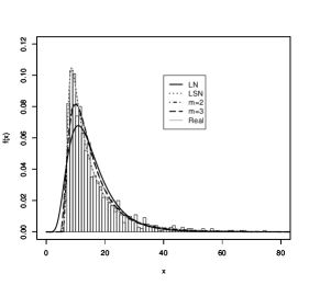
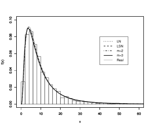
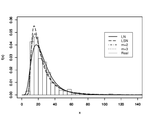
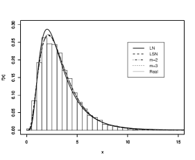
Figure 5 shows that, in Data 1 and Data 3, the fitted LN distribution poorly estimates the left tail of the distribution. The height of the mode is not well estimated by the LN distribution in Data 1, Data 2 and Data 3 and, by the LSN distribution in Data 1. The proposed models do not estimate well the height of the mode in Data 3 but they do it much better than the LN distribution. LSN and the proposed model are comparable in Data 2 and Data 4 and they are comparable to the LN in Data 4, showing the flexibility of the LCFUSN distribution.

Figure 5: Estimated densities of $LN$, $LSN$, $LCFUSN_{1,2}$ and $LCFUSN_{1,3}$ models for Data 1(top left), Data 2 (top right), Data 3 (bottom left) and Data 4 (bottom right).

5.2 Case Study 1: Selecting model using entropy

Quoting [14], pp. 623, “ $\dots$ in making inference on the basis of partial information we must use that probability distribution which has the maximum entropy subject to whatever is known. This is the only unbiased assignment we can make; to use any other would amount to arbitrary assumption of information which by hypothesis we do not have.”

In this section we analyze the USA monthly precipitation data recorded from 1895 to 2007 by fitting LCFUSN distributions with different values for $m$. This data is available at the National Climatic Data Center (NCDC) and consists of 1,344 observations of the US precipitation index (PCL). Our main goal here is to consider the Jaynes’s principle to select the best model, that is, we select the model that maximizes the entropy. Models are also chosen using two well-known tools for model selection, the conditional predictive ordinate (SlnCPO) and the deviance information criterion (DIC). Denote by $Y_{i}$ the precipitation index in the $i$th month. In [22] the authors fitted the LSN (say, the LCFUSN with $m=1$) and different LCFUSN distributions and evaluate the gain in assuming a higher dimensional skewing function to analyze the data. We assume the same models, that is, we consider that $Y_{i}\mid\mu,\sigma^{2},\delta\sim LCFUSN_{1,m}(\mu,\sigma^{2},\delta{\bf{1}}_{m,1})$ and postulate for all parameters the same flat prior distributions elicited in Subsection 5.1. We also let $m$ to vary from $m=1$ (LSN) to $m=5$. We name $M_{i}$ the model for which we assume $m=i$. By considering such specifications and assuming the posterior means, in [22] it is obtained very close plug-in estimates of the true density for all $m$ as can be noticed in Figure 6.

Figure 6: Fitted LCFUSN and LSN densities, precipitation data.

Table 2 shows the 95% HPD, SlnCPO, DIC and the entropy comparing all models. The entropy was computed using the two different approaches presented in Section 4.

Table 2: Model selection statistics, Precipitation data.

Model	$E(\delta\mid{\bf Y})$	Mean Entropy	$95\%$ HPD	Plug-in Entropy	DIC	SlnCPO
$LN$	$-$	$0.883$	$[0.844;0.924]$	$0.890$	$62.69$	$-0.8815$
$LSN$	$-0.947$	$1.143$	$[0.963;1.313]$	$1.158$	$-13.19$	$-0.83766$
$m=2$	$-0.686$	$1.164$	$[1.101;1.236]$	$1.230$	$-36.96$	$-0.83545$
$m=3$	$-0.570$	$1.256$	$[1.160;1.348]$	$1.314$	$-112.40$	$-0.83765$
$m=4$	$-0.497$	$1.467$	$[1.364;1.566]$	$1.539$	$-321.10$	$-0.84144$
$m=5$	$-0.446$	$1.777$	$[1.675;1.880]$	$1.815$	$-895.30$	$-0.81057$

We notice that the mean entropy increases with the complexity of the model. Moreover, the HPDs for models $LSN$ and $M_{2}$ point out that the amount of information in our system is quite similar and this same conclusion holds for models $M_{2}$ and $M_{3}$. The HDPs for models $M_{4}$ and $M_{5}$ do not intersect, indicating that the entropy of these two models are significantly different. By using the maximum entropy principle we decide for $M_{5}$ as the best model, and this decision is the same we make using standard procedures for model selection, such as DIC and the SlnCPO. Moreover, we notice that, at least in this example, the entropy and the DIC have similar behavior and leads to the same decision. It should be observed that the $LN$ model, which is the most common choice for this type of data analysis, provides the poorest fit among all models, as shown by the model selection statistics DIC and SlnCPO as well as by the Shannon entropy.

5.3 Case Study 2: Clustering with KL divergence

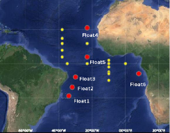
Climate in some Brazilian areas are directly influenced by some features of Atlantic ocean such as surface temperature and humidity. To better understand how such influence occurs, a system of 21 floats were installed over different regions of Atlantic ocean (see Figure 7) and some of such features are daily measured.

Figure 7: Selected floats in Atlantic ocean.

We choose six of this floats and consider the daily relative humidity from September 11th, 1997 to September 22nd, 2014. Such floats (their locations are in parenthesis) are named Float1 (19S 34W), Float2 (4S 32W), Float3(8S 30W), Float4(21N 23W), Float5 (4N 23W) and Float6 (6S 8E) and are the big balls in Figure 7. Data are available at URL:http://goosbrasil.org/. Our goal is to verify if the relative humidity level in all these regions have similar behavior. The importance of such kind of study from the statistical point of view is to permit us to cluster information in similar floats looking for improvements in the estimates. On the other hand, from the economic perspective, it can be considered to define an optimal design for the system used to measure information in Atlantic area excluding some of the floats which brings similar information.

We assume two different distributions to model the humidity $Y$ in each float. In the first case we consider that $Y_{i}\mid\mu,\sigma^{2}\sim LN(\mu,\sigma^{2})$, which is a standard assumption to analyze this data. As an alternative we also assume that $Y_{i}\mid\mu,\sigma^{2},\mbox{\boldmath$\Delta$}\sim LCFUSN_{1,2}(\mu,\sigma^{2},\delta{\bf{1}}_{1,2})$. As in Case Study 1, flat prior distributions for the parameters are considered.

Table 3 provides the DIC comparing the fitted models for each float as well as the KL divergence between the two distributions under consideration. Considering the method introduced in [21] and assuming that distributions are similar whenever the KL divergence is up to the cut point $0.14$, we concluded that the LN and LCFUSN are very similar to describe the humidity behavior in each float. Despite of this, the DIC points out that the LCFUSN distribution is a better model for all floats. Therefore, in the following, our analysis is based on the LCFUSN distribution only.

Table 3: DIC and Kullback-Leibler divergence between LCFUSN and LN distributions for each float.

Float	DIC-LN	DIC-LCFUSN	$D(LCFUSN||LN)$	$D(LN||LCFUSN)$
1	$-6,310$	$-20,500$	$0.0047$	$0.0040$
2	$-9,703$	$-17,930$	$0.0017$	$0.0039$
3	$-9,708$	$-15,070$	$0.0007$	$0.0010$
4	$-4,859$	$-104,100$	$0.0365$	$0.0806$
5	$-8,079$	$-20,790$	$0.0064$	$0.0055$
6	$-2,530$	$-25,120$	$0.0307$	$0.0663$

Table 4 shows the KL divergence comparing the LCFUSN distributions $f_{i}$ and $f_{j}$ of floats $i$ and $j$. Since the KL divergence is asymmetric, we will assume that data of different floats have the same distribution, and thus could be clustered, whenever $D(f_{i}|f_{j})$ and $D(f_{j}|f_{i})$ are both up to $0.14$. It can be noticed from Table 4 that the relative humidity measured on floats 3 and 6 are similar, hence one of them could be excluded from the system without losing substantial information. In fact, the predictive distributions based on data measured on Floats 3 and 6 are quite similar to that obtained when we merge the data from these floats.

Table 4: Kullback-Leibler divergence between $f_{i}$ and $f_{j}$.

$Float$	1	2	3	4	5	6
1	$-$	$0.2534$	$0.5427$	$0.1446$	$1.0543$	$0.6560$
2	$0.1390$	$-$	$0.1646$	$0.3346$	$0.8198$	$0.4549$
3	$0.2433$	$0.1602$	$-$	$0.2471$	$0.3117$	${\bf{0.1249}}$
4	$0.1761$	$0.6623$	$0.5055$	$-$	$0.4862$	$0.3795$
5	$0.6707$	$1.0787$	$0.4345$	$0.2134$	$-$	$0.1766$
6	$0.4235$	$0.5416$	${\bf{0.1323}}$	$0.2033$	$0.0937$	$-$

Table 5 shows the mean and the variance of the prior predictive distribution for the relative humidity in all these cases. As can be noticed, the predictive distributions have very close means and similar variance. However, when we merged the data, the variability on the humidity on Float 6 is underestimated by a small amount. That probably happens because data in Float 6 discloses a high degree of skewness as can be noticed from Table 6. It is also noteworthy that the merged data better capture the features of data measured on Float 3.

Table 5: Prior predictive mean and variance based on data in Floats 3 and 6 and the merged.

	$E(Y)$	$Var(Y)$
Float 3	$78.66$	$14.91$
Float 6	$80.45$	$17.20$
Merged	$79.56$	$15.41$

Table 6: Posterior summaries data of Floats 3 and 6 and the merged data.

	$\mu$		$\sigma$		$\delta$
	Mean	St. Dev.	Mean	St. Dev.	Mean	St. Dev.	$95\%$HPD
Float 3	$4.410$	$0.005$	$0.059$	$0.002$	$-0.493$	$0.037$	$[-0.564,-0.428]$
Float 6	$4.477$	$0.004$	$0.083$	$0.003$	$-0.687$	$0.007$	$[-0.699,-0.672]$
Merged	$4.420$	$0.005$	$0.062$	$0.002$	$-0.521$	$0.031$	$[-0.575,-0.457]$

6 Final Comments

In this paper we presented some results related to the entropy and KL divergence of two classes of multivariate distributions recently introduced in the literature, the multivariate log-canonical fundamental skew-normal (LCFUSN) and the canonical fundamental skew-normal (CFUSN) distributions. We also obtained the MI for distributions in these families. Bayesian approach is considered to estimate the entropy and KL divergence. Such measures were computed in two different ways, obtaining their posterior distribution and using the plug-in method where the posterior means of the parameters were assumed as estimators. To illustrate the use of some results, entropy was used for model comparison. We concluded that Jaynes’s principle selected the same model as DIC and CPO. KL divergence was used to compare the distribution of relative humidity collected in scattered floats on different regions of Atlantic ocean. We concluded that the humidity in some floats has a very similar behavior and some of such floats could be removed from the system if the only goal were to measure the humidity.

An interesting topic for future research is to consider some generalizations of Shannon entropy, such as Mathai’s generalized entropy and Rényi’s entropy, in the $LCFUSN$ and $CFUSN$ families of distributions. Mathai’s generalized entropy was used in [16], who proved that the pathway model can be obtained by optimizing such entropy.

7 Appendix

In this section we present the proofs of propositions that appear in the text.

Proof of Proposition 2: First note that if ${\bf X}\sim CFUSN(\mbox{\boldmath$\mu$},\bf{\Sigma},\bf\Delta)$, then ${\bf X}=\mbox{\boldmath$\mu$}+\bf{\Sigma}^{1/2}{\bf Z}$, where ${\bf Z}\sim CFUSN(\bf\Delta)$, and $H_{{\bf X}}=\frac{1}{2}\ln|\bf{\Sigma}|+H_{{\bf Z}}$. Thus we only need to calculate $H_{{\bf Z}}$. Consider the pdf given in Equation (5). Thus, we have $H_{CFUSN(\bf{\Delta})}=-E(\ln\phi(Z))-E_{{\bf Z}}[\ln(2^{m}\Phi_{m}(\mbox{\boldmath$\Delta$}^{\prime}{\bf Z}|\mbox{\boldmath$\Delta$}^{*}))]=\frac{n}{2}\ln 2\pi+\frac{1}{2}\sum_{i=1}^{n}E(Z_{i}^{2})-E_{{\bf Z}}[\ln(2^{m}\Phi_{m}(\mbox{\boldmath$\Delta$}^{\prime}{\bf Z}|\mbox{\boldmath$\Delta$}^{*}))].$ The proof is concluded by noticing that $\sum_{i=1}^{n}E(Z_{i}^{2})=E({\bf Z}^{\prime}{\bf Z})=\mbox{\boldmath$\mu$}_{0}\mbox{\boldmath$\mu$}_{0}+tr(\mbox{\boldmath$\Sigma$}_{0})$, where $\mbox{\boldmath$\mu$}_{0}=E({\bf Z})$ and $\mbox{\boldmath$\Sigma$}_{0}=Var({\bf Z})$.

Proof of Proposition 4(ii): By definition it follows that

$$D(f_{{\bf Y}}||f_{{\bf Z}})=-H_{CFUSN_{n,m_{2}}(\mbox{\boldmath$\mu$}_{2},\mathbf{\Sigma}_{2},\mathbf{\Delta_{2}})}-\int_{\mathbb{R}^{n}}f_{{\bf Y}}({\bf y})\ln[f_{{\bf Z}}({\bf y})]d{\bf y}.$$ (25)

The integral at the right side of Equation (25) can be calculated as follows:

$$\int_{\mathbb{R}^{n}}f_{{\bf Y}}({\bf y})\ln[f_{{\bf Z}}({\bf y})]d{\bf y}=-\sum_{i=1}^{n}E_{{\bf Y}}(Y_{i}){-\frac{1}{2}}\ln|\mbox{\boldmath$\Sigma$}_{1}|-\frac{n}{2}\ln 2\pi$$ (26)

$$- \frac{1}{2}E_{{\bf Y}}\left(({\bf Y}-\mbox{\boldmath$\mu$}_{1})^{\prime}\mbox{\boldmath$\Sigma$}_{1}^{-1}({\bf Y}-\mbox{\boldmath$\mu$}_{1})\right)+E_{{\bf Y}}\left(\ln\left[2^{m_{1}}\Phi_{m_{1}}(\mbox{\boldmath$\Delta$}_{1}^{\prime}\mbox{\boldmath$\Sigma$}_{1}^{-\frac{1}{2}}({\bf Y}-\mbox{\boldmath$\mu$}_{1})|\mbox{\boldmath$\Delta$}_{1}^{*})\right]\right),$$

where ${\bf Y}\sim CFUSN_{n,m_{2}}(\mbox{\boldmath$\mu$}_{2},\mathbf{\Sigma}_{2},\mbox{\boldmath$\Delta$}_{2})$ and $Y_{i}$ is the $i$-th component of ${\bf Y}$. Replacing $(\ref{inf3})$ in $(\ref{entrorelativa2})$ we have that

$$D(f_{{\bf Y}}||f_{{\bf Z}})=\frac{1}{2}\ln\left[\frac{\mbox{\boldmath$\Sigma$}_{1}}{\mbox{\boldmath$\Sigma$}_{2}}\right]+E_{{\bf Y}}\left(\ln\left[\frac{2^{m_{2}-m_{1}}\Phi_{m_{2}}(\mbox{\boldmath$\Delta$}_{2}^{\prime}\mbox{\boldmath$\Sigma$}_{2}^{-\frac{1}{2}}({\bf Y}-\mbox{\boldmath$\mu$}_{2})|\mbox{\boldmath$\Delta$}_{2}^{*})}{\Phi_{m_{1}}(\mbox{\boldmath$\Delta$}_{1}^{\prime}\mbox{\boldmath$\Sigma$}_{1}^{-\frac{1}{2}}({\bf Y}-\mbox{\boldmath$\mu$}_{1})|\mbox{\boldmath$\Delta$}_{1}^{*})}\right]\right)$$

$$+\frac{1}{2}E_{{\bf Y}}\left(({\bf Y}-\mbox{\boldmath$\mu$}_{1})^{\prime}\mbox{\boldmath$\Sigma$}_{1}^{-1}({\bf Y}-\mbox{\boldmath$\mu$}_{1})\right)-\frac{E_{{\bf Y}_{0}}({\bf Y}_{0}^{\prime}{\bf Y}_{0})}{2},$$

where ${\bf Y}_{0}\sim CFUSN_{n,m}(0,{\bf I}_{n},\mbox{\boldmath$\Delta$})$. The proof follows from Equation (15) by noticing that $E_{{\bf Y}_{0}}({\bf Y}_{0}^{\prime}{\bf Y}_{0})=\mbox{\boldmath$\mu$}_{0}\mbox{\boldmath$\mu$}_{0}+tr(Var({\bf Y}_{0}))$, where $\mbox{\boldmath$\mu$}_{0}=E({\bf Y}_{0})$.

References

• [1] Ahmed, N. A. & Gokhale, D. V. (1989). Entropy expressions and their estimators for multivariate distributions. IEEE Trans. Inform. Theory, 35, 688-692.
• [2] Arellano-Valle, R. B., Contreras-Reyes, J. E. & Genton, M. G. (2013). Shannon entropy and mutual information for multivariate skew-elliptical distributions. Scandinavian Journal of Statistics, 40, 42-62.
• [3] Arellano-Valle, R. B. & Genton, M. G. (2005). On fundamental skew distributions. Journal of Multivariate Analysis, 96(1), 93-116.
• [4] Azzalini, A. (1985). A class of distributions which includes the normal ones. Scandinavian Journal of Statistics, 12, 171-178.
• [5] Azzalini, A., Dal Cappello, T. & Kotz, S. (2002). Log-skew-normal and log-skew-t distributions as models for family income data. Journal of Income Distribution, 11(3,4), 12-20.
• [6] Azzalini, A. & Dalla Valle, A. (1996). The multivariate skew-normal distribution. Biometrika, 83, 715-726.
• [7] Bernardo, J. M. (1979). Reference posterior distributions for Bayesian inference (with discussion). Journal of the Royal Statistical Society, Series B, 41, 113-147.
• [8] Contreras-Reyes, J. E. & Arellano-Valle, R. B. (2012). Kullback-Leibler divergence measure for multivariate skew-normal distributions. Entropy, 14(9), 1606-1626.
• [9] Cover, T. M. and Thomas, J. A. (2006). Elements of information theory, 2nd ed. Wiley, New Jersey.
• [10] Gupta, M. & Srivastava, S. (2010). Parametric Bayesian estimation of differential entropy and relative entropy Entropy, 12, 818–843.
• [11] Gutiérrez-Peña, E. & Muliere, P. (2004). Conjugate priors represent strong pre-experimental assumptions. Scandinavian Journal of Statistics, 31, 2325-246.
• [12] Javier, W. R. & Gupta, A. K. (2008). Mutual information for the mixture of two multivariate normal distributions. Far East Journal of Theoretical Statistics, 26, 47-58.
• [13] Javier, W. R. & Gupta, A. K. (2009). Mutual information for certain multivariate distributions. Far East Journal of Theoretical Statistics, 29, 39-51.
• [14] Jaynes, E. T. (1957). Information Theory and Statistical Mechanics. The Physical Review, 106(4), 620-630.
• [15] Jaynes, E. T. (1968). Prior probabilities. IEEE Transactions Systems, Science and Cybernetics, 4, 227-291.
• [16] Jose, K. K. & Naik, S.R. (2008). A class of asymmetric pathway distributions and an entropy interpretation. Physica A, 387, 6943-6951.
• [17] Kullback, S. (1978). Information theory and statistics, Dover Edition, Gloucester.
• [18] Kullback, S. & Leibler, R. A. (1951). On information and sufficiency. Annals of Mathematical Statistics, 22, 79-86.
• [19] Larsen K, Petersen JH, Budtz-Jøitalic-ø\orgensen E and Endahl L. Interpreting parameters in the logistic regression model with random effects. Biometrics. 2000; 56: 909–914.
• [20] Marchenko, Y. V. & Genton, M. G. (2010). Multivariate log-skew-elliptical distributions with applications to precipitation data. Environmetrics, 21, 318-340.
• [21] McCulloch, R. E. (1989). Local model influence. Journal of the American Statistical Associ- ation, 84(406), 473-478.
• [22] Queiroz, M. M., Loschi, R. H. & Silva, R. W. C. (2016). Multivariate Log-Skewed Distributions with normal kernel and its Applications. Statistics, 50(1), 157-175.
• [23] Santos, C.C., Loschi, R.H. and Arellano-Valle, R.B. (2013). Parameter Interpretation in Skewed Logistic Regression with Random Intercept. Bayesian Analysis, 8(2), 381–410.
• [24] Sahu, S. K. (2002). Bayesian Estimation and model selection choice in item response models. Journal of Statistical Computation and Simulation, 72(3), 217-232.
• [25] Shannon, C. E. (1948). A mathematical theory of communication. The Bell System Technical Journal, 27, 379-423, 623-656.
• [26] Yuan, A. & Clarke, B. S. (1999). A minimally informative likelihood for decision analysis: Illustration and robstness. Canadian Journal of Statistics, 27, 649–665.