Effects of grain growth on the interstellar polarization curve

Abstract

We apply the time evolution of grain size distributions by accretion and coagulation found in our previous work to the modelling of the wavelength dependence of interstellar linear polarization. We especially focus on the parameters of the Serkowski curve $K$ and $\lambda_{\max}$ characterizing the width and the maximum wavelength of this curve, respectively. We use aligned silicate and non-aligned carbonaceous spheroidal particles with different aspect ratios $a/b$. The imperfect alignment of grains with sizes larger than a cut-off size $r_{V,\rm cut}$ is considered. We find that the evolutionary effects on the polarization curve are negligible in the original model with commonly used material parameters (hydrogen number density $n_{\mathrm{H}}=10^{3}$ cm^-3, gas temperature $T_{\mathrm{gas}}=10$ K, and the sticking probability for accretion $S_{\mathrm{acc}}=0.3$). Therefore, we apply the tuned model where the coagulation threshold of silicate is removed. In this model, $\lambda_{\max}$ displaces to the longer wavelengths and the polarization curve becomes wider ($K$ reduces) on time-scales $\sim(30-50)(n_{\mathrm{H}}/10^{3}\mathrm{cm}^{-3})^{-1}$ Myr. The tuned models at $T\mathrel{\mathchoice{\vbox{\offinterlineskip\halign{\hfil$\displaystyle#$\hfil\cr<\cr\sim\cr}}}{\vbox{\offinterlineskip\halign{\hfil$\textstyle#$\hfil\cr<\cr\sim\cr}}}{\vbox{\offinterlineskip\halign{\hfil$\scriptstyle#$\hfil\cr<\cr\sim\cr}}}{\vbox{\offinterlineskip\halign{\hfil$\scriptscriptstyle#$\hfil\cr<\cr\sim\cr}}}}30(n_{\mathrm{H}}/10^{3}\mathrm{cm}^{-3})^{-1}$ Myr and different values of the parameters $r_{V,\rm cut}$ can also explain the observed trend between $K$ and $\lambda_{\max}$. It is significant that the evolutionary effect appears in the perpendicular direction to the effect of $r_{V,\rm cut}$ on the $K$ – $\lambda_{\max}$ diagram. Very narrow polarization curves can be reproduced if we change the type of particles (prolate/oblate) and/or vary $a/b$.

1 Introduction

Interstellar dust plays a crucial role in the evolution of galaxies (Dwek, 1998; Zhukovska et al., 2008; Draine, 2009; Inoue, 2011; Asano et al., 2014). Traditionally, dust models are tested using interstellar extinction curves. As a result, the constraints on the grain size distribution (e.g. Mathis et al. 1977; Zubko et al. 1996; Weingartner & Draine 2001) and evolution of grain materials (e.g. Jones et al. 1990; Li & Greenberg 1997; Cecchi-Pestellini et al. 2010; Jones et al. 2013; Mulas et al. 2013; Cecchi-Pestellini et al. 2014; Köhler et al. 2014) can be obtained.

Less popular modelling of interstellar polarization makes it possible to investigate not only interstellar dust but also interstellar magnetic fields. The wavelength dependence of polarization is used for estimates of grain size and composition (Mathis 1986; Kim & Martin 1995; Voshchinnikov et al. 2013) while the polarizing efficiency and distribution of position angles give information about grain alignment and magnetic field (Fosalba et al. 2002; Whittet et al. 2008; Voshchinnikov & Das 2008; Reissl et al. 2014; see also Andersson 2012 and Voshchinnikov 2012 for recent reviews).

In this paper, we examine the variation of interstellar polarization, using our recent results of grain size distribution (Hirashita & Voshchinnikov 2014) and optical constants of grain materials (Jones et al. 2013).

Jones et al. (2013) proposed a new two-material interstellar dust model, consisting of amorphous silicate and hydrocarbon dust. In this model, the visual – near infrared (IR) extinction is mainly produced by large forsterite-type silicate grains with metallic iron nano-particle inclusions (a-Sil_Fe) and large aliphatic-type carbonaceous grains (a-C(:H)). The typical radii of grains are 0.1 – 0.2 ${\mu}\rm{m}$. During the life-cycle silicate and carbonaceous particles can accumulate the thin mantles consisting of aromatic-type carbon (a-C).

Hirashita & Voshchinnikov (2014, hereafter HV14) have investigated the time evolution of grain size distribution due to the accretion and coagulation in an interstellar cloud and examined whether dust grains processed by these mechanisms can explain observed variation of extinction curves in the Milky Way. It was found that, if we consider accretion and coagulation with commonly used material parameters, the model fails to explain the Milky Way extinction curves. This discrepancy was resolved by adopting a ‘tuned’ model, in which coagulation of carbonaceous dust is less efficient and that of silicate is more efficient with the coagulation threshold being removed. The tuned model is also consistent with the relation between silicon depletion (an indicator of accretion) and $R_{V}$ (the ratio of total to selective extinction, an indicator of grain growth), and the correlation between ultraviolet (UV) slope $c_{2}$ in the parametric fit of extinction curve according to Fitzpatrick & Massa (2007) and $R_{V}$.

Here, we take the size distributions obtained by HV14 as a starting point for our analysis of the time evolution of interstellar polarization curve. We use the model of spheroidal particles that was earlier applied to interpret the interstellar extinction and polarization (Voshchinnikov & Das 2008; Das et al. 2010; Voshchinnikov et al. 2013).

The paper is organized as follows. The description of observations and the model is given in Section 2. Section 3 contains the results of the modelling of wavelength dependence of polarization $P(\lambda)$ and the relation between the width of the curve $P(\lambda)$ and the position of the maximum polarization $\lambda_{\rm max}$. Sections 4 and 5 present the discussion of results and conclusions.

2 Interstellar polarization

Interstellar linear polarization is caused by the linear dichroism of the interstellar medium due to the presence of non-spherical aligned grains. Dust grains must have sizes close to the wavelength of the incident radiation and specific magnetic properties to efficiently interact with the interstellar magnetic field.

2.1 Observations: Serkowski curve

The wavelength dependence of polarization $P(\lambda)$ in the visible part of spectrum is described by an empirical formula suggested by Serkowski (1973)

$$P(\lambda)/P_{\max}=\exp[-K\ln^{2}(\lambda_{\max}/\lambda)].$$ (1)

This formula has three parameters: the maximum degree of polarization $P_{\max}$, the wavelength corresponding to it $\lambda_{\max}$ and the coefficient $K$ characterizing the width of the Serkowski curve. The values of $P_{\max}$ in the diffuse interstellar medium usually do not exceed 10%, and the mean value of $\lambda_{\max}$ is 0.55 ${\mu}\rm{m}$ (Serkowski et al. 1975).

The parameter $K$ determines the half-width of the normalized interstellar linear polarization curve

$$W=\lambda_{\rm max}/\lambda_{-}-\lambda_{\rm max}/\lambda_{+},$$ (2)

where $\lambda_{-}<\lambda_{\max}<\lambda_{+}$ and $P(\lambda_{+})=P(\lambda_{-})=P_{\max}/2$. The relation between $W$ and $K$ is as follows:

$$W=\exp[(\ln 2/K)^{1/2}]-\exp[-(\ln 2/K)^{1/2}].$$ (3)

Treating $K$ as a third free parameter of the Serkowski curve, Whittet et al. (1992) fit the relation between $K$ and $\lambda_{\max}$ in the Milky Way as

$$K=(1.66\pm 0.09)\lambda_{\max}+(0.01\pm 0.05).$$ (4)

2.2 Modelling

Interpretation of the wavelength dependence of interstellar polarization includes calculations of the extinction cross sections of rotating partially aligned non-spherical particles. In early studies, an unphysical model of infinitely long cylinders was applied. More realistic is the spheroidal model of grains with the shape of these axisymmetric particles being characterized by the only parameter — the ratio of the major to minor semi-axis $a/b$. This model is particularly promising for interpretation of the interstellar polarization and extinction data (see Voshchinnikov 2012 for review).

We represent the interstellar dust grains by a mixture of silicate and carbonaceous homogeneous spheroids of different sizes and orientations. A solution to the light scattering problem for such particles has been given by Voshchinnikov & Farafonov (1993).

The linear polarization of unpolarized stellar radiation produced by aligned rotating spheroidal particles after the passage through a dust cloud with the uniform magnetic field is

$$P(\lambda)=\sum_{j}\int\limits_{0}^{D}\int\limits_{r_{V,\min,j}}^{r_{V,\max,j}}\overline{C}_{{\rm pol},j}(m_{\lambda,j},a_{j}/b_{j},r_{V},\lambda)\,$$

$$\times n_{j}(r_{V})\,dr_{V}\,dl\times 100\,\%\,,$$ (5)

$$\overline{C}_{{\rm pol},j}={\frac{2}{\pi^{2}}}{\int\limits_{0}^{\pi/2}}{\int\limits_{0}^{\pi}}{\int\limits_{0}^{\pi/2}}\frac{1}{2}(C^{\rm TM}_{{\rm ext},j}-C^{\rm TE}_{{\rm ext},j})\,$$

$$\times f_{j}(\xi,\beta,...)\,\cos 2{\psi}\,d{\varphi}\,d{\omega}\,d{\beta}\,,$$ (6)

where $D$ is the distance to the star, $\lambda$ the wavelength, $m_{\lambda,j}$, $a_{j}/b_{j}$ $n_{j}(r_{V})$ are the refractive index, aspect ratio and size distribution of spheroidal particles of the $j$th kind ($j=$Si for silicate and $j=$C for carbonaceous dust, respectively), $r_{V}$ is the radius of a sphere whose volume is equal to that of the spheroid (for prolate particles, $r_{V}=\sqrt[3]{ab^{2}}$, and for oblate ones, $r_{V}=\sqrt[3]{a^{2}b}$), ${r_{V,\min,j}}$ and ${r_{V,\max,j}}$ are the minimum and maximum radii, respectively, and $C^{\rm TM,\,TE}_{{\rm ext},j}$ the extinction cross-sections for two polarization modes depending on the particle orientation relative to the electric vector of incident radiation (Bohren & Huffman 1983). The angle $\psi$ can be expressed through $\varphi,\omega,\beta,\Omega$ (see the definitions of the angles and relations between them, e.g., in Das et al. 2010), and finally ${f}_{j}(\xi,\beta,...)$ is the distribution of the particles of the $j$th kind over orientations.

2.2.1 Size distribution

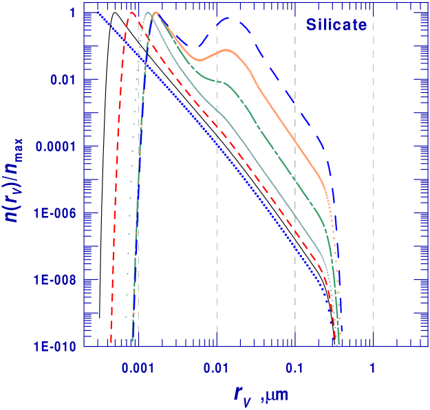
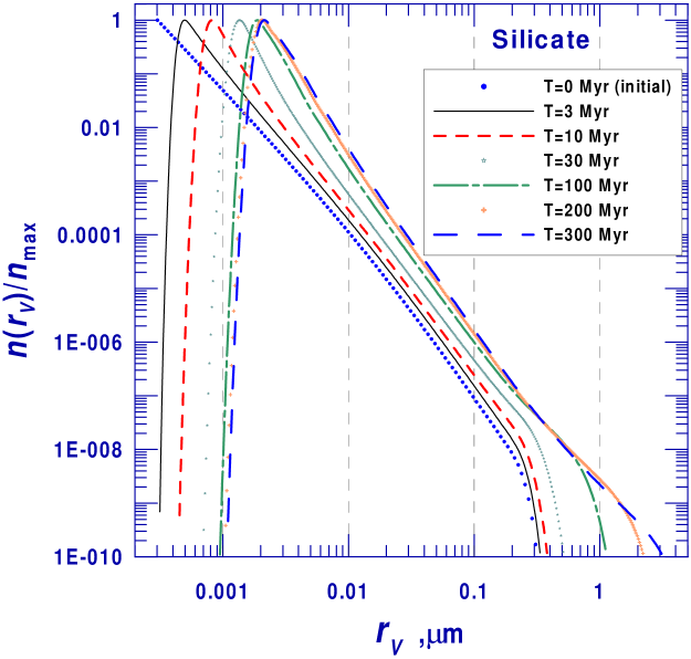
Figure 1: Evolution of grain size distribution for silicate dust. The grain size distribution is normalized to the maximum. Effects of evolution of grain size distribution are shown for original (left panel) and tuned (right panel) models at $T=3$, 10, 30, 100, 200 and 300 Myr. The initial condition is shown by the dotted line.

HV14 calculated the time evolution of grain size distribution by accretion and coagulation based on the formulation by Hirashita (2012). Silicate and carbonaceous dust were treated as separate grain species.

The growth time-scale of grain radius for accretion is determined by the gas-phase abundance of the key elements Si and C (assumed to be proportional to the metallicity $Z$), hydrogen number ($n_{\mathrm{H}}$) density, gas temperature ($T_{\mathrm{gas}}$) and the sticking probability for accretion ($S_{\mathrm{acc}}$). We adopt the following values for quantities: $Z=\mathrm{Z}_{\sun}$, $n_{\mathrm{H}}=10^{3}$ cm^-3, $T_{\mathrm{gas}}=10$ K, and $S_{\mathrm{acc}}=0.3$.

HV14 considered thermal (Brownian) motion and turbulent motion as a function of grain mass and solved a discretized coagulation equation (see Hirashita 2012 for details). The coagulation was assumed to occur if the relative velocity was below the coagulation threshold given by Hirashita & Yan (2009). It was also adopted that the sticking coefficient for coagulation $S_{\mathrm{coag}}$ was 1.

As an initial grain size distribution (at time $T=0$), HV14 choose the size distributions of silicate and carbonaceous dust that fits the mean Milky Way extinction curve for $R_{V}=3.1$ (Weingartner & Draine, 2001). The initial size distribution of silicate grains is shown by the dotted line in Fig. 1.

Using the size distributions obtained for silicate and carbonaceous dust, HV14 calculated the evolution of extinction curve and found that the prominent variation of extinction caused by increasing accretion occurs at $<30$ Myr. After that, the evolution of extinction curve is driven only by coagulation, which flattens the extinction curve and makes $R_{V}$ larger. Observations indicate that even for large $R_{V}\approx 4.4$, the carbon bump around 0.22 $\micron$ is clear and the UV extinction rises with a positive curvature. However, the theoretical predictions show that at large $R_{V}$ (i.e. after significant coagulation at $T>100$ Myr), the carbon bump disappears. This implies that coagulation is in reality not so efficient as assumed in the model for carbonaceous dust. There is another discrepancy: the observed $A_{V}/N_{\mathrm{H}}$ tends to decrease drastically as $R_{V}$ increases, while it does not decrease significantly after pronounced coagulation at $T>100$ Myr.This is because silicate stops to coagulate at $r_{V}\sim 0.03~{}\micron$, which is still too small to affect the UV opacity.

In summary, the observational data indicate (i) that carbonaceous dust should be more inefficient in coagulation than assumed, and (ii) that silicate should grow beyond $r_{V}\sim 0.03~{}\micron$ (the growth is limited by the coagulation threshold velocity). Therefore, for a better fit the observational data, HV14 also tried models with $S_{\mathrm{coag}}<1$ for carbonaceous dust and no coagulation threshold for silicate dust as a tuned model. Such a tuning is acceptable if we consider uncertainties in grain properties. The removal of the coagulation threshold may be justified if the grains have fluffy structures that absorb the collision energy efficiently, and/or are coated with sticky materials such as water ice (Ormel et al. 2009; Hirashita & Li 2013).

In the tuned model, the coagulation efficiency was decreased by a factor of 2 by adopting $S_{\mathrm{coag}}=0.5$ for carbonaceous dust, while $S_{\mathrm{coag}}=1$ for silicate was kept. Silicate grains were assumed to coagulate whenever they collide (no coagulation threshold). The accretion efficiency ($S_{\mathrm{acc}}=0.3$) was not changed for both silicate and carbonaceous dust to minimize the fine tuning. This is called ‘tuned model’, while we call the original model with $S_{\mathrm{coag}}=1$ and the coagulation threshold ‘original model without tuning’.

The evolution of silicate grain size distribution for the tuned model is shown in Fig. 1 (right panel). Compared with the dust distributions in the original model without tuning (Fig. 1, left panel), the grains grow further, even beyond 1 $\micron$ at $>100$ Myr. As shown later, silicate grains in the large-size tail of size distribution are of crucial importance in explanation of observed polarization.

We use size distribution of silicate and carbonaceous grains obtained by HV14 but replace spherical particles by spheroids of the same mass. The uncertainties of grain shape to spheroidal has only a minor influence on accretion and coagulation compared with the change of $S_{\mathrm{acc}}$ and $S_{\mathrm{coag}}$. Therefore, that we simply use HV14’s results with an assumption of $a=r_{v}$.

2.2.2 Materials

Jones (2012a, b, c) published a comprehensive analysis of the compositional properties of hydrogenated amorphous carbons. It includes the consideration of the evolution of carbon solids from hydrogen rich aliphatic grains (a-C:H, sp³ bonded) to hydrogen poor aromatic grains (a-C, sp² bonded), calculations of the complex refractive indexes as a function of the material band gap, and investigation of size-dependent properties. Later, Jones et al. (2013) found refractive indexes of amorphous silicates using the mixture of amorphous forsterite with different amount of metallic iron (a-Sil_Fe) and Köhler et al. (2014) added iron sulfide in this mixture.

In modelling, we choose the refractive index ’silicate$\_$FoFe10.RFI’ for amorphous silicates with 10% volume fraction of Fe (equivalent to $\sim$70% of the cosmic Fe) and the data for an a-C(:H) material with a band gap $E_{g}=2.5$ eV. The optical constants were taken from Jones et al. (2013) and Jones (2012b) for silicate and carbon, respectively. The chosen carbon material seems to represent the bulk of the carbonaceous dust formed around evolved stars (A. P. Jones, private communication). We ignore the possible evolutionary sequence for the silicates because of the large vagueness of this problem and the size dependence of refractive indexes since it is unimportant in the visual part of spectrum. Note that the used materials are different from those in HV14. However, this fact as well as the replacement of spherical particles by spheroidal ones are of no significance for normalized extinction curves, e.g., the difference in $R_{V}$ does not exceed 0.1 – 0.2.

2.2.3 Alignment

We assume that the spheroidal grains are partly aligned so that their major axes rotate in a plane ($\varphi$ is the angle of rotation) and their angular momentum J precesses around the direction of the magnetic field ($\omega$ is the precession angle, $\beta$ the opening angle of the precession cone). Such alignment is called the imperfect Davis–Greenstein (IDG) alignment. It is described by the distribution function ${f}_{{\rm IDG},j}(\xi,\beta)$ depending only on the orientation parameter $\xi$ and the angle $\beta$ for particles of the $j$th kind (Hong & Greenberg 1980):

$${f}_{{\rm IDG},j}(\xi,\beta)=\frac{\xi\sin\beta}{(\xi^{2}\cos^{2}\beta+\sin^{2}\beta)^{3/2}}.$$ (7)

The parameter $\xi$ depends on the particle size $r_{V}$, the imaginary part of the magnetic susceptibility of a dust grain $\chi^{\prime\prime}=\varkappa\omega_{\rm d}/T_{\rm d}$, where $\omega_{\rm d}$ is the angular velocity of the particle, hydrogen number density $n_{\rm H}$, magnetic field strength $B$, and temperatures of dust $T_{\rm d}$ and gas $T_{\rm gas}$ as

$$\xi^{2}=\frac{r_{V}+\delta_{0,\,j}^{\rm IDG}(T_{\rm d}/T_{\rm gas})}{r_{V}+\delta_{0,\,j}^{\rm IDG}},$$ (8)

where

$$\delta_{0,\,j}^{\rm IDG}=8.23\,10^{23}\frac{\varkappa B^{2}}{n_{\rm H}T_{\rm gas}^{1/2}T_{\rm d}}\,{\mu}\rm{m}.$$ (9)

In the IDG mechanism, smaller grains which are powerful polarizers are aligned better than larger grains (see Eq. (8)). In order to reduce the polarizing efficiency below the observed values, it is possible to increase the minimum cut-off in grain size distribution ${r_{V,\min,j}}$ (e.g. Das et al. 2010) or to assume that small particles are randomly oriented (e.g. Draine & Fraisse 2009).

Because the grain size distribution is fixed in our model (see Section 2.2.1) we suggest the following modified IDG alignment function with reduced alignment of small grains (see also Mathis 1986):

$${f}_{j}(\xi,\beta,...)=\left[1-\exp(-r_{V}/r_{V,\rm cut})^{3}\right]\,\times\,{f}_{{\rm IDG},j}(\xi,\beta)\,,$$ (10)

where $r_{V,\rm cut}$ is a cut-off parameter. The alignment function (10) gives a smooth switch from non-aligned to aligned grains in comparison with abrupt jump suggested by Draine & Fraisse (2009).

Though the silicate and carbonaceous particles comparably contribute to extinction, the polarization is assumed to be produced only by silicate particles. Such an assumption has been earlier done by Chini & Krügel (1983) and Mathis (1986), and recently has got additional support in the work of Voshchinnikov et al. (2012) who found a correlation between the observed interstellar polarization degree and the abundance of silicon in dust grains. Polarization in IR features also supports the idea of separate populations of polarizing (silicate) and non-polarizing (carbonaceous) grains. This follows from the observed polarization of silicate features at 10 $\,{\mu}\rm{m}$ and 18 $\,{\mu}\rm{m}$ and the lack of polarization in the 3.4 $\,{\mu}\rm{m}$ hydrocarbon feature (Hough & Aitken 2004; Chair et al. 2006; see also discussion in Li et al. 2014).

3 Results

We made calculations for prolate and oblate homogeneous spheroids consisting of silicate and amorphous carbon. The particles of 59 sizes in the range from $r_{V,\min}=0.001\,{\mu}\rm{m}$ to $r_{V,\max}=1\,{\mu}\rm{m}$ were utilized. The extinction and polarization curves have been calculated for 77 wavelengths in the range from $\lambda=0.2\,{\mu}\rm{m}$ to $\lambda=5\,{\mu}\rm{m}$. We next determine parameters of the Serkowski curve $P_{\max}$, $\lambda_{\max}$, and $K$. In this paper, we focus on the normalized curves $P(\lambda)/P_{\max}$ and the relation between the width of the polarization curve and the position of its maximum. These characteristics of the Serkowski curve are mainly determined by the size distribution $n_{\rm Si}(r_{V})$ and the cut-off parameter $r_{V,\rm cut}$ of silicate particles and weakly depend on the degree ($\delta_{0}^{\rm IDG}$) and direction ($\Omega$) of the particle orientation. Therefore, we fix the alignment parameters: $\delta_{0,\,{\rm Si}}^{\rm IDG}=0.5\,{\mu}\rm{m}$, $\delta_{0,\,{\rm C}}^{\rm IDG}=0.01\,{\mu}\rm{m}$, and $\Omega=60\deg$.

3.1 Wavelength dependence

3.1.1 Linear polarization

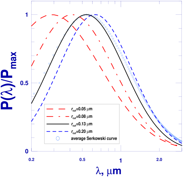
Figure 2: Normalized wavelength dependence of linear polarization for the initial size distribution ($T=0$ Myr, see Fig. 1). The average observational Serkowski curve ($\lambda_{\max}=0.55\,\mu$m, $K=0.92$) is plotted using the open circles. The theoretical curves were calculated for prolate spheroids with $a/b=3$. The characteristics of theoretical curves are: $r_{V,\,\rm cut}=0.05\,\mu$m, $\lambda_{\max}=0.289\,\mu$m, $K=0.64$; $r_{V,\,\rm cut}=0.08\,\mu$m, $\lambda_{\max}=0.415\,\mu$m, $K=0.88$; $r_{V,\,\rm cut}=0.13\,\mu$m, $\lambda_{\max}=0.538\,\mu$m, $K=1.07$ and $r_{V,\,\rm cut}=0.20\,\mu$m, $\lambda_{\max}=0.628\,\mu$m, $K=1.16$.

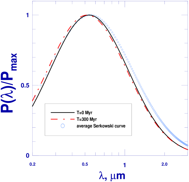
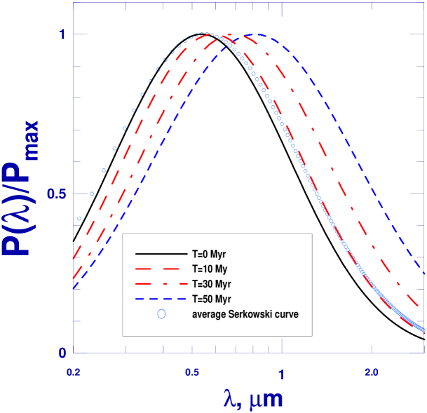
Figure 3: Normalized wavelength dependence of interstellar linear polarization. Effects of evolution of grain size distribution on curves $P(\lambda)$ are shown for the original model without tuning (left) and the tuned (right) model. The average observational Serkowski curve ($\lambda_{\max}=0.55\,\mu$m, $K=0.92$) is plotted using the open circles. The theoretical curves were calculated for the model: prolate spheroids, $a/b=3$, $r_{V,\,\rm cut}=0.13\,\mu$m. The parameter $r_{V,\,\rm cut}$ for initial curve was chosen in such a manner in order to be closer to observational curve. The characteristics of theoretical curves are: $T=0$ Myr, $\lambda_{\max}=0.538\,\mu$m, $K=1.07$; original model: $T=300$ Myr, $\lambda_{\max}=0.519\,\mu$m, $K=1.04$; tuned model: $T=10$ Myr, $\lambda_{\max}=0.588\,\mu$m, $K=1.05$; $T=30$ Myr, $\lambda_{\max}=0.689\,\mu$m, $K=0.95$; $T=50$ Myr, $\lambda_{\max}=0.812\,\mu$m, $K=0.81$.

First of all, we calculated the polarization curve $P(\lambda)/P_{\max}$ for the initial size distribution of silicate and carbonaceous dust. If we assume that grains of all sizes are aligned according to IDG mechanism ($r_{V,\,\rm cut}=0$ in Eq. (10)), the polarization peaks at far-UV ($\lambda_{\max}<0.2\,\mu$m). In order to fit the average observational Serkowski curve ($\lambda_{\max}=0.55\,\mu$m and $K=0.92$ according to Eq. (4)), we increase parameter $r_{V,\,\rm cut}$. Figure 2 shows how the variations of $r_{V,\,\rm cut}$ influence the polarization curve. It is clearly seen that both $\lambda_{\max}$ and $K$ grow with growing the cut-off parameter, i.e. for larger values of $r_{V,\,\rm cut}$, the curve $P(\lambda)$ becomes narrower and its maximum shifts to longer wavelengths (see Section 3.2 for more discussion the relation between $K$ and $\lambda_{\max}$). A plausible result would be achieved for $r_{V,\,\rm cut}=0.13\,\mu$m (Fig. 2).

We choose the model with $r_{V,\,\rm cut}=0.13\,\mu$m presented in Fig. 2 as the basic one. For this model and the assumed values of $\delta_{0}^{\rm IDG}$ and $\Omega$, the ratio of total extinction to selective one $R_{V}=3.39$ and the polarizing efficiency of the interstellar medium $P_{\max}/A_{V}=1.54$ %/mag. (usually $P_{\max}/A_{V}\mathrel{\mathchoice{\vbox{\offinterlineskip\halign{\hfil$\displaystyle#$\hfil\cr<\cr\sim\cr}}}{\vbox{\offinterlineskip\halign{\hfil$\textstyle#$\hfil\cr<\cr\sim\cr}}}{\vbox{\offinterlineskip\halign{\hfil$\scriptstyle#$\hfil\cr<\cr\sim\cr}}}{\vbox{\offinterlineskip\halign{\hfil$\scriptscriptstyle#$\hfil\cr<\cr\sim\cr}}}}3$ %/mag. for interstellar polarization, Serkowski et al. 1975). The average size of polarizing dust grains b$\langle r_{V,{\rm pol,\,Si}}\rangle=0.17\,{\mu}\rm{m}$. It can be found using the following expression:

$$\langle r_{V,{\rm pol,\,Si}}\rangle=\frac{\displaystyle\int\limits_{r_{{}_{V},{\rm cut}}}^{r_{{}_{V},\max}}r_{V}n_{\rm Si}(r_{V})\,{d}r_{V}}{\displaystyle\int\limits_{r_{{}_{V},{\rm cut}}}^{r_{{}_{V},\max}}n_{\rm Si}(r_{V})\,{d}r_{V}}\,.$$ (11)

With increasing $r_{V,\,\rm cut}$ from $0.05\,\mu$m to $0.20\,\mu$m, $\lambda_{\max}$ and $K$ grow from $0.289\,\mu$m to $0.628\,\mu$m and from 0.64 to 1.16, respectively, while $\langle r_{V,{\rm pol,\,Si}}\rangle$ increases from $0.08\,{\mu}\rm{m}$ to $0.23\,{\mu}\rm{m}$.

Now we can investigate the changes in polarization curve owing to the evolution of grain size distribution. Our results are shown in Fig. 3 for original model without tuning (left panel) and tuned model (right panel). As is clearly seen from Fig. 3, the evolutionary effects are negligible in the original model: the difference between initial polarization curve and that at $T=300$ Myr is very small and comparable to observational errors. The reason is that the significant changes of grain size occur only at the smallest sizes for silicate grains which do not contribute to the observed polarization (Fig. 1, left panel) while the largest size of silicate grains is always $\sim 0.3\,{\mu}\rm{m}$. However, there are time variations in extinction curves, especially in the UV bump because the carbonaceous dust can grow beyond $0.3\,{\mu}\rm{m}$ (see discussion in HV14).

In the tuned model, the coagulation threshold of silicate is removed, which leads to the appearance of rather large grains (Fig. 1, right panel). As a consequence, the curves $P(\lambda)$ show a detectable shift from the initial curve just after $T\mathrel{\mathchoice{\vbox{\offinterlineskip\halign{\hfil$\displaystyle#$\hfil\cr>\cr\sim\cr}}}{\vbox{\offinterlineskip\halign{\hfil$\textstyle#$\hfil\cr>\cr\sim\cr}}}{\vbox{\offinterlineskip\halign{\hfil$\scriptstyle#$\hfil\cr>\cr\sim\cr}}}{\vbox{\offinterlineskip\halign{\hfil$\scriptscriptstyle#$\hfil\cr>\cr\sim\cr}}}}10$ Myr (Fig. 3, right panel). During first stage ($\sim 30-50$ Myr), the maximum of polarization displaces to longer wavelengths and the polarization curve becomes wider ($K$ reduces). Further evolution shows that $\lambda_{\max}$ continues to grow but the curve $P(\lambda)$ becomes narrower ($K$ increases). It is evident that the polarization curves obtained for $T\mathrel{\mathchoice{\vbox{\offinterlineskip\halign{\hfil$\displaystyle#$\hfil\cr>\cr\sim\cr}}}{\vbox{\offinterlineskip\halign{\hfil$\textstyle#$\hfil\cr>\cr\sim\cr}}}{\vbox{\offinterlineskip\halign{\hfil$\scriptstyle#$\hfil\cr>\cr\sim\cr}}}{\vbox{\offinterlineskip\halign{\hfil$\scriptscriptstyle#$\hfil\cr>\cr\sim\cr}}}}50$ Myr do not reproduce the available observations (see Fig. 5 and discussion in Section 3.2).

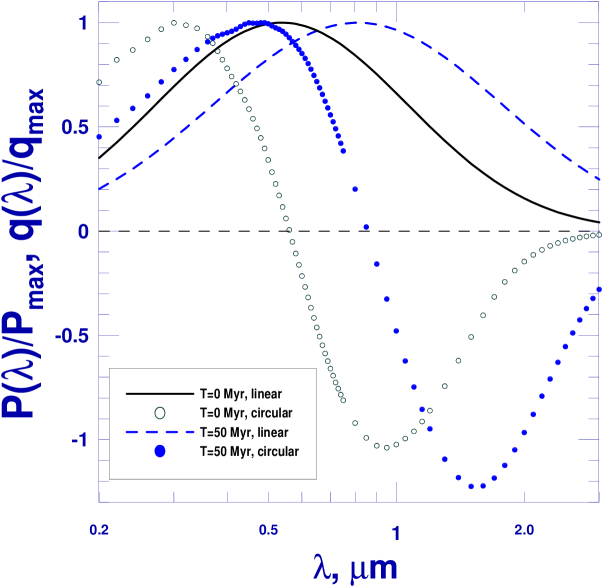
Figure 4: Normalized wavelength dependence of interstellar linear and circular polarization. The curves $P(\lambda)P_{\max}$ and $q(\lambda)/q_{\max}$ are shown for the initial curve ($T=0$ Myr) and in the case of tuned model ($T=50$ Myr).

3.1.2 Circular polarization

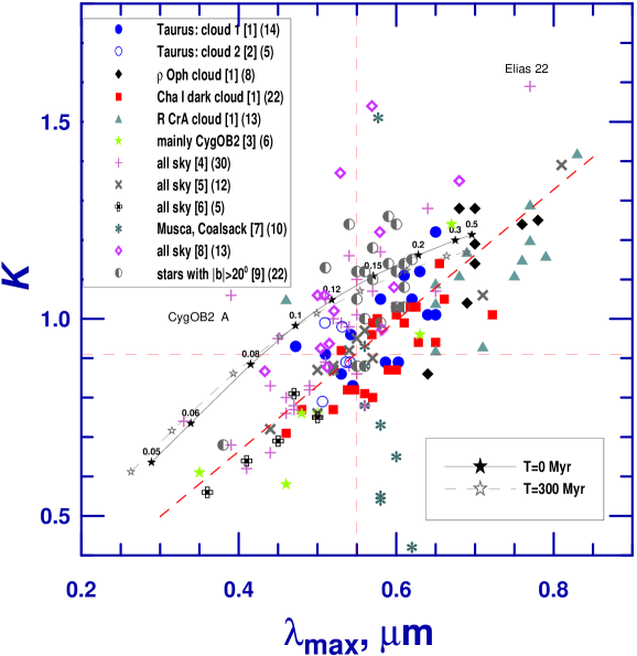
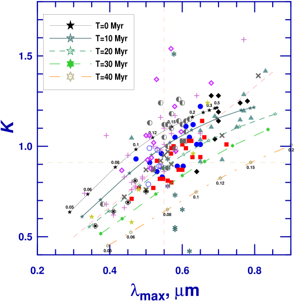
Figure 5: Parameter $K$ of Serkowski curve versus the wavelength $\lambda_{\max}$ of the maximum linear polarization. The symbols indicate the observational data for 160 stars in the Milky Way. The sources of data and number of stars are given in the legend in square brackets and parenthesis, respectively ([1] – Voshchinnikov et al. 2013; [2] – Whittet et al. 2001; [3] – Martin et al. 1992; [4] – Whittet et al. 1992; [5] – Wilking et al. 1980; [6] – Wilking et al. 1982; [7] – Andersson & Potter 2007; [8] – Clayton et al. 1995; [9] – Larson 1999). Stars ($\star$) connected with solid and dashed lines illustrate the results of modelling for original model without tuning (left panel) and tuned model (right panel). Model: prolate spheroids with $a/b=3$ are adopted. The values of $r_{V,\,\rm cut}$ are shown for the initial size distribution ($T=0$ Myr) and in the case of tuned model ($T=40$ Myr). Horizontal and vertical dashed lines correspond to the average Serkowski curve ($\lambda_{\max}=0.55\,\mu$m, $K=0.92$). Inclined dashed line corresponds to the relation $K=1.66\lambda_{\max}$ (see Eq. (4)).

We also calculated the wavelength dependence of interstellar circular polarization $q(\lambda)$ for the initial size distribution and for the tuned model. These curves are plotted in Fig. 4 together with the corresponding linear polarizations $P(\lambda)$. As usual, the circular polarization has two extremes (see e.g. Voshchinnikov 2004; Siebenmorgen et al. 2014). They shift with time to longer wavelengths The wavelength where the curve $q(\lambda)$ changes the sign is close to the wavelength where the curve $P(\lambda)$ has the maximum (i.e., $\lambda_{c}\approx\lambda_{\max}$), which, in particular, confirms the correctness of used data for refractive indexes.

3.2 Relation between $K$ and $\lambda_{\max}$

Now we discuss the models in the context of the sample of Milky Way polarization curves with the determined parameters of Serkowski curve collected from the literature. The starting list contained 57 stars located in the nearby dark clouds in Taurus and Chamaeleon, around the stars $\rho$ Oph and R CrA (Voshchinnikov et al. 2013). It was extended up to 160 objects using the data published by Martin et al. (1992), Whittet et al. (1992), Wilking et al. (1980), Wilking et al. (1982), Andersson & Potter (2007), Clayton et al. (1995), and Larson (1999). The observational data are plotted in Fig. 5 using different symbols. The stars are located in different parts of the sky and at different distances. Although we excluded the stars with rotation of position angle, perhaps, some stars are observed through two or more clouds. Sometimes, this may distort the values of $K$ and $\lambda_{\max}$ in comparison with the single cloud situation (Clarke & Al-Roubaie 1984; Clarke 2010). Nevertheless, the bulk of observational points concentrates in the middle part of Fig. 5 and shows a clear correlation between parameters $K$ and $\lambda_{\max}$. The typical errors are $\sim 0.01\,{\mu}\rm{m}$ for $\lambda_{\max}$ and $\sim 0.1$ for $K$. Almost all stars located above and below the general trend (excluding may be two objects CygOB2 A and Elias 22) are normal stars. The observational data for the stars with $K$ and $\lambda_{\max}$ beyond the general trend as well as the regional variations require more careful analysis which will be made in a separate paper. Note also that stars at high galactic latitudes obtained by Larson (1999) do not stand out between others.

Theoretical dependence constructed for the initial model and different $r_{V,\,\rm cut}$ demonstrate the simultaneous growth of $K$ and $\lambda_{\max}$ but passes slightly above the major cluster of observational data. For the used model (prolate spheroids, $a/b=3$) there is another problem with the explanation of the observational points with $\lambda_{\max}\mathrel{\mathchoice{\vbox{\offinterlineskip\halign{\hfil$\displaystyle#$\hfil\cr>\cr\sim\cr}}}{\vbox{\offinterlineskip\halign{\hfil$\textstyle#$\hfil\cr>\cr\sim\cr}}}{\vbox{\offinterlineskip\halign{\hfil$\scriptstyle#$\hfil\cr>\cr\sim\cr}}}{\vbox{\offinterlineskip\halign{\hfil$\scriptscriptstyle#$\hfil\cr>\cr\sim\cr}}}}0.7\,\mu$m. This is difficult even for models with very large values of $r_{V,\,\rm cut}$. An attempt to remedy the situation using the evolved size distribution in the original model without tuning does not meet a success (Fig. 5, left panel): the shift of points is very insignificant. However, if we apply the tuned model, the major part of observational data can be fitted. Figure 5 (right panel) shows that the tuned models with $T\mathrel{\mathchoice{\vbox{\offinterlineskip\halign{\hfil$\displaystyle#$\hfil\cr<\cr\sim\cr}}}{\vbox{\offinterlineskip\halign{\hfil$\textstyle#$\hfil\cr<\cr\sim\cr}}}{\vbox{\offinterlineskip\halign{\hfil$\scriptstyle#$\hfil\cr<\cr\sim\cr}}}{\vbox{\offinterlineskip\halign{\hfil$\scriptscriptstyle#$\hfil\cr<\cr\sim\cr}}}}40$ Myr allow simultaneously to increase the maximum wavelength and the width of polarization curve ($K$ reduces) in comparison with the initial model.

Very narrow polarization curves ($K>1.2$) as well as observational points located above the model with $T=0$ Myr can be reproduced if we change the type of particles (prolate/oblate) or/and to vary the particle shape (parameter $a/b$) (Fig. 6). The replacement of prolate spheroids by oblate ones leads to a growth of both $\lambda_{\max}$ and $K$ (the curves become narrower). The same dependence takes place if we decrease the aspect ratio $a/b$ for prolate spheroids. The opposite situation occurs for oblate spheroids: $\lambda_{\max}$ and $K$ grow if $a/b$ is increased.

4 Discussion

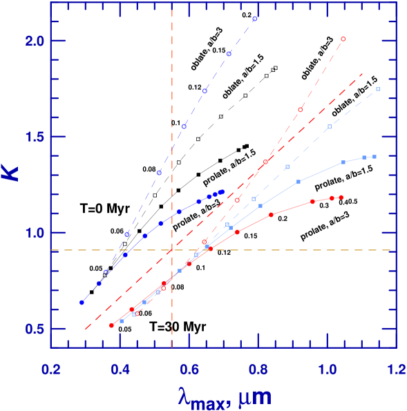
Figure 6: Parameter $K$ of Serkowski curve versus the wavelength $\lambda_{\max}$ of the maximum linear polarization. The results of modelling for the initial size distribution ($T=0$ Myr) and for tuned model with $T=30$ Myr are shown in the case of prolate and oblate spheroids with $a/b=1.5$ and 3. The results are plotted using filled symbols and solid lines for prolate spheroids and using open symbols and dashe lines for oblate spheroids. The values of $r_{V,\,\rm cut}$ are given for the extreme models. Horizontal and vertical dashed lines correspond to the average Serkowski curve ($\lambda_{\max}=0.55\,\mu$m, $K=0.92$). Inclined dashed line corresponds to the relation $K=1.66\lambda_{\max}$ (see Eq. (4)).

Our modelling shows that the observed wavelength dependence of the interstellar linear polarization and the correlation between $K$ and $\lambda_{\max}$ can be reproduced using imperfectly aligned silicate spheroidal grains. Time variations of the particle size distribution are determined by the processes of grain accretion and coagulation in the tuned model where the coagulation threshold of silicate is removed. The original model without tuning predicts minor variations for polarization curves and must be rejected.

Our model has two main parameters: the cut-off size $r_{V,\rm cut}$ in the alignment function and grain size distribution function determined by the time of grain processing in the molecular clouds $T$. Increasing $r_{V,\rm cut}$ enables us to explain simultaneously the increase of the maximum wavelength $\lambda_{\max}$ and the reduction of the width of polarization curve (to increase parameter $K$). As it is seen from Fig. 5, the cut-off size must be rather large ($r_{V,\rm cut}\mathrel{\mathchoice{\vbox{\offinterlineskip\halign{\hfil$\displaystyle#$\hfil\cr>\cr\sim\cr}}}{\vbox{\offinterlineskip\halign{\hfil$\textstyle#$\hfil\cr>\cr\sim\cr}}}{\vbox{\offinterlineskip\halign{\hfil$\scriptstyle#$\hfil\cr>\cr\sim\cr}}}{\vbox{\offinterlineskip\halign{\hfil$\scriptscriptstyle#$\hfil\cr>\cr\sim\cr}}}}0.2\,{\mu}\rm{m}$) in order to explain the observational data with $\lambda_{\max}\mathrel{\mathchoice{\vbox{\offinterlineskip\halign{\hfil$\displaystyle#$\hfil\cr>\cr\sim\cr}}}{\vbox{\offinterlineskip\halign{\hfil$\textstyle#$\hfil\cr>\cr\sim\cr}}}{\vbox{\offinterlineskip\halign{\hfil$\scriptstyle#$\hfil\cr>\cr\sim\cr}}}{\vbox{\offinterlineskip\halign{\hfil$\scriptscriptstyle#$\hfil\cr>\cr\sim\cr}}}}0.6\,{\mu}\rm{m}$. However, reducing particle aspect ratio $a/b$ and replacing prolate spheroids with oblates, one permits to decrease significantly the value of $r_{V,\rm cut}$ (Fig. 6). Changes in $r_{V,\rm cut}$ may be attributed to the selective action of grain alignment by the anisotropic radiation fluxes (radiative torque alignment). This mechanism is effective if $r_{V}\mathrel{\mathchoice{\vbox{\offinterlineskip\halign{\hfil$\displaystyle#$\hfil\cr>\cr\sim\cr}}}{\vbox{\offinterlineskip\halign{\hfil$\textstyle#$\hfil\cr>\cr\sim\cr}}}{\vbox{\offinterlineskip\halign{\hfil$\scriptstyle#$\hfil\cr>\cr\sim\cr}}}{\vbox{\offinterlineskip\halign{\hfil$\scriptscriptstyle#$\hfil\cr>\cr\sim\cr}}}}\lambda_{\rm eff}/2\pi$ (Draine 2011), so the trend in Fig. 5 may reflect the systematic changes of starlight background energy distribution (increase of the fraction of red stars with corresponding growth of the effective wavelength $\lambda_{\rm eff}$) from bottom left to up right corner.

Using the initial model with $T=0$ Myr and varying $r_{V,\rm cut}$, particle type and shape we can not reproduce a part of observational data located at the lower left corner and middle part of Fig. 5 ($\lambda_{\max}\mathrel{\mathchoice{\vbox{\offinterlineskip\halign{\hfil$\displaystyle#$\hfil\cr<\cr\sim\cr}}}{\vbox{\offinterlineskip\halign{\hfil$\textstyle#$\hfil\cr<\cr\sim\cr}}}{\vbox{\offinterlineskip\halign{\hfil$\scriptstyle#$\hfil\cr<\cr\sim\cr}}}{\vbox{\offinterlineskip\halign{\hfil$\scriptscriptstyle#$\hfil\cr<\cr\sim\cr}}}}0.6\,{\mu}\rm{m}$, $K\mathrel{\mathchoice{\vbox{\offinterlineskip\halign{\hfil$\displaystyle#$\hfil\cr<\cr\sim\cr}}}{\vbox{\offinterlineskip\halign{\hfil$\textstyle#$\hfil\cr<\cr\sim\cr}}}{\vbox{\offinterlineskip\halign{\hfil$\scriptstyle#$\hfil\cr<\cr\sim\cr}}}{\vbox{\offinterlineskip\halign{\hfil$\scriptscriptstyle#$\hfil\cr<\cr\sim\cr}}}}1.1$). In this case, to interpret observations we need to apply the tuned models with evolution time $T\mathrel{\mathchoice{\vbox{\offinterlineskip\halign{\hfil$\displaystyle#$\hfil\cr<\cr\sim\cr}}}{\vbox{\offinterlineskip\halign{\hfil$\textstyle#$\hfil\cr<\cr\sim\cr}}}{\vbox{\offinterlineskip\halign{\hfil$\scriptstyle#$\hfil\cr<\cr\sim\cr}}}{\vbox{\offinterlineskip\halign{\hfil$\scriptscriptstyle#$\hfil\cr<\cr\sim\cr}}}}30$ Myr. These models fit the major part of observed extinction curves except for several stars with $R_{V}>5$ where the models with $T=200-300$ Myr are required (see Fig. 7 in HV14). Note that for stars with $R_{V}>5$ multi-wavelength polarimetric data are not available, so they do not enter into our sample.

The restriction on the duration of accretion and coagulation in the tuned models obtained by us ($T\mathrel{\mathchoice{\vbox{\offinterlineskip\halign{\hfil$\displaystyle#$\hfil\cr<\cr\sim\cr}}}{\vbox{\offinterlineskip\halign{\hfil$\textstyle#$\hfil\cr<\cr\sim\cr}}}{\vbox{\offinterlineskip\halign{\hfil$\scriptstyle#$\hfil\cr<\cr\sim\cr}}}{\vbox{\offinterlineskip\halign{\hfil$\scriptscriptstyle#$\hfil\cr<\cr\sim\cr}}}}30$ Myr) does not contradict to the lifetime of molecular clouds found from chemical modelling (3 – 6 Myr; Pagani et al. 2011) and dynamical simulation (5 – 25 Myr; Dobbs & Pringle 2013). We should also emphasize that the time-scales of accretion and coagulation both scale with $\propto n_{\mathrm{H}}^{-1}$ (HV14), i.e. if we adopt $n_{\mathrm{H}}=10^{4}$ cm^-3 instead of $10^{3}$ cm^-3, the same size distributions are reached at ten times shorter time.

5 Conclusions

The main results of the paper can be formulated as follows.

1. We applied the grain size distributions found by Hirashita & Voshchinnikov (2014) to the explanation of the interstellar linear polarization. Time evolution of grain size distribution is due to the accretion and coagulation in an interstellar cloud. We considered the model with commonly used material parameters and tuned model, in which coagulation of carbonaceous dust is less efficient and that of silicate is more efficient with the coagulation threshold being removed.

2. To calculate the polarization, we used the model of homogeneous silicate and carbonaceous spheroidal particles with different aspect ratios $a/b$ and imperfect alignment. It was assumed that polarization is mainly produced by large silicate particles with sizes $r_{V}\mathrel{\mathchoice{\vbox{\offinterlineskip\halign{\hfil$\displaystyle#$\hfil\cr>\cr\sim\cr}}}{\vbox{\offinterlineskip\halign{\hfil$\textstyle#$\hfil\cr>\cr\sim\cr}}}{\vbox{\offinterlineskip\halign{\hfil$\scriptstyle#$\hfil\cr>\cr\sim\cr}}}{\vbox{\offinterlineskip\halign{\hfil$\scriptscriptstyle#$\hfil\cr>\cr\sim\cr}}}}r_{V,\rm cut}$. We calculated the wavelength dependence of polarization and determined parameters of the Serkowski curve $K$ and $\lambda_{\max}$ describing the width of the polarization curve and the wavelength at the maximum polarization, respectively.

3. It was found that the evolutionary effects are negligible in the original model without tuning. This is a consequence of the insignificant evolutionary changes of large silicate grains contributing to observed polarization. In the tuned model, the coagulation threshold of silicate is removed, and at $\sim(30-50)(n_{\mathrm{H}}/10^{3}\mathrm{cm}^{-3})^{-1}$ Myr, the maximum of polarization displaces to the longer wavelengths and the polarization curve becomes wider ($K$ reduces).

4. We compiled parameters of Serkowski curve for a sample of 160 lines of sight and compared theory and observations. The observed trend between $K$ and $\lambda_{\max}$ can be explained if we use the tuned models with $T\mathrel{\mathchoice{\vbox{\offinterlineskip\halign{\hfil$\displaystyle#$\hfil\cr<\cr\sim\cr}}}{\vbox{\offinterlineskip\halign{\hfil$\textstyle#$\hfil\cr<\cr\sim\cr}}}{\vbox{\offinterlineskip\halign{\hfil$\scriptstyle#$\hfil\cr<\cr\sim\cr}}}{\vbox{\offinterlineskip\halign{\hfil$\scriptscriptstyle#$\hfil\cr<\cr\sim\cr}}}}(30-40)(n_{\mathrm{H}}/10^{3}\mathrm{cm}^{-3})^{-1}$ Myr and different values of the cut-off size $r_{V,\rm cut}$. It is significant that the evolutionary effect appears in the perpendicular direction to the effect of $r_{V,\rm cut}$ on $K$ – $\lambda_{\max}$ diagram. Very narrow polarization curves ($K>1.2$) can be reproduced if we change the type of particles (prolate/oblate) and/or to vary the particle shape (parameter $a/b$).

References

- Andersson (2012) Andersson, B. - G., 2012, arXiv: 1208.4393
- Andersson & Potter (2007) Andersson, B. - G., & Potter, S. B., 2007, ApJ, 665, 369
- Asano et al. (2014) Asano, R., Takeuchi, T. T., Hirashita, H., & Nozawa, T., 2014, MNRAS, 440, 134
- Bohren & Huffman (1983) Bohren C. F., Huffman D. R., 1983, Absorption and Scattering of Light by Small Particles, Wiley, New York
- Cecchi-Pestellini et al. (2010) Cecchi-Pestellini, C., Cacciola, A., Iatì , M. A., Saija, R., Borghese, F., Denti, P., Giusto, A., & Williams D. A., 2010, MNRAS, 408, 535
- Cecchi-Pestellini et al. (2014) Cecchi-Pestellini, C., Casu, S., Mulas, G., & Zonca, A., 2014, ApJ, 785:41
- Chair et al. (2006) Chair, J. E., Adamson, A. J., Whittet, D. C. B., Chrysostomou, A., Hough, J. H., Kerr, T. H., Mason, R. E., Roche, P. F., & Wright, G., 2006, ApJ, 651, 268
- Chini & Krügel (1983) Chini, R., & Krügel, E., 1983, A&A, 117, 289
- Clarke (2010) Clarke, D., 2010, Stellar Polarimetry, Wiley-VCH, Weinheim
- Clarke & Al-Roubaie (1984) Clarke, D., & Al-Roubaie, A., 1984, MNRAS, 206, 729
- Clayton et al. (1995) Clayton, G. C., Wolff, M. J., Allen, R. G., & Lupie, O. L., 1995, ApJ, 445, 957
- Das et al. (2010) Das, H. K., Voshchinnikov, N. V., & Il’in, V. B., 2010, MNRAS, 404, 265
- Dobbs & Pringle (2013) Dobbs, C. L., & Pringle, J. E., 2012, MNRAS, 432, 653
- Draine (2009) Draine B. T., 2009, in Henning Th., Grün E., Steinacker J., eds, ASP Conf. Ser. 414, Cosmic Dust – Near and Far. Astron. Soc. Pac., San Francisco, p. 453
- Draine (2011) Draine B. T., 2011, Physics of the Interstellar and Intergalacic Medium, Princeton Univ. Press, Princeton
- Draine & Fraisse (2009) Draine, B. T., & Fraisse, A. A., 2009, ApJ, 626, 1
- Dwek (1998) Dwek E., 1998, ApJ, 501, 643
- Fitzpatrick & Massa (2007) Fitzpatrick, E. L., & Massa, D., 2007, ApJ, 663, 320
- Fosalba et al. (2002) Fosalba, P., Lazarian, A., Prunet, S., & Tauber, J.A., 2002, ApJ, 564, 762
- Hirashita (2012) Hirashita, H., 2012, MNRAS, 422, 1263
- Hirashita & Li (2013) Hirashita, H., & Li, Z.-Y., 2013, MNRAS, 434, L70